Nanomechanically induced transparency in -symmetric optical cavities
Abstract
In this paper, we analytically present the phenomena of nanomechanically induced transparency (NMIT) and transmission rate in a parity-time-symmetric (-symmetric) opto-nanomechanical system (ONMS) where a levitated dielectric nanospheres is trapped near the antinodes closest to right mirror of passive cavity which further coupled to an active cavity via hoping factor. We find that the phenomenon of NMIT may be generated from the output probe field in the presence of an effective opto-nanomechanical coupling between the cavity field and the nanosphere, whose steady-state position is influenced by the Coulomb interaction between the cavity mirror and the nanosphere. In addition, the width and height of the transparency window can be controlled through the effective optomechanical coupling, which is readily adjusted by altering changing the nanosphere’s radius and the Coulomb interaction. One of the most interesting result is the transition NMIT behavior in -symmetric and broken -symmetric regime. We show that the presence of nanosphere in the passive cavity enhances the width and transmission rate of NMIT window in passive-passive regime and in passive-active regime, a notable decrease of sideband amplification has been observed. These results show that our scheme may find some potential applications for optical signal processing an and quantum information processing.
I Introduction
One basic axiom in canonical quantum mechanics requires that the Hermiticity of every operator be directly related with a physical observable. In addition, the spectrum of a Hermitian operator is guaranteed to be real. Bender and colleagues, however, discovered a class of Hamiltonians that are non-Hermitian with fully real spectra provided they fulfil combined parity-time () symmetry bender1 ; bender2 . Open physical systems with balanced amplification (gain) and absorption (loss) are known as -symmetric systems. If a critical value is exceeded for the parameter controlling the degree of non-Hermiticity, such systems exhibit spontaneous symmetry breaking. The eigenvalues of such system become complex beyond this threshold even though BPENG . -symmetry has been widely investigated theoretically and experimentally demonstrated in various physical systems, with quantum optics emerging as the most versatile platform to explore -symmetric applications. Up to now, -symmetric systems have been extensively observed in quantum information processing (QIP) and quantum optics, opening up novel applications including soliton active controlling RDBA ; FNAZ enhancing photon blockade JLRY , realizing quantum chaos XYLU , strengthening optical nonlinearity JLXZ ; SKGA and so on. In addition, -symmetric Hamiltonian has also been experimentally realized in many physical systems BPNG ; AREG ; LFENG ; LCHAN .
Although -symmetry in optomechanical system enhances various quantum optical effects when balanced through the loss with extra gain, there still are opposite directions in which environmental loss play a vital role. As an analog of electromagnetically induced transparency (EIT), optomechanically induced transparency (OMIT) is the most notable of these directions Agr ; SAZY ; SAUM . It is notable that the value of the cavity decay rate must be large in order to observe optomechanically-induced-transparency (OMIT). It is also worth mentioning that an extra gain in optomechanical system is taken into account to deviate from OMIT behavior, even leads to optomechanically-induced absorption (OMIA) or inverted-OMIT. As of right now, other additional coupled systems such as two and three-level atoms SAZY ; YXYF ; YTYL ; YHJC ; YCTS , Bose-Einstein condensates BFRS ; RITS ; YKAA , magnon S1 ; S2 ; S3 ; S4 etc., are still needed for the enhancing quantum properties like OMIT, entanglement, Furthermore, levitated nanosphere, trapped inside an optical cavity, has also been considered to discuss many quantum features such as gravitational wave detection KRHG ; AAGA and quantum ground state cooling KNBF ; MJFP ; CDER ; RIOP . Therefore, a natural question arises. Can an optically trapped nanosphere play an important role in -symmetric coupled cavity system?
In this paper, we address this question by considering -symmetric system that comprise two coupled cavities. The passive cavity contain a levitated nanosphere. Particularly, we show: (i) existence of an NMIT window in the red-sideband region and a small dip in the blue-sideband region in a single cavity system; (ii) NMIT-like spectrum in addition to sharp absorptive peak in the blue-sideband region when we consider an active cavity with no loss/gain; (iii) an inverted NMIT which strongly depends on the modulated interaction between the cavity and the nanosphere; and (iv) a reversed opto-nanomechanical coupling dependence of the transmission rate.
The rest of the manuscript is organized as follows. In section II, the model and the corresponding system dynamics of the opto-nanomechanical system are presented. In section III, we theoretically discuss the NMIT and the transmission of the ONMS. The section IV concludes our paper.
II The model and the dynamics
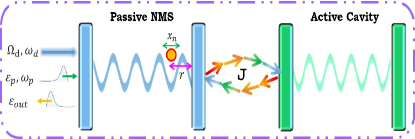
The current opto-nanomechanical system is comprised of two connected cavities, as depicted in Figure 1, where the first (passive) cavity contains a nanosphere. The cavity bosonic creation and annihilation operators are represented as and while cavity decay rate is . The second cavity is an active cavity with gain rate and is represented by the bosonic creation (annihilation) as . A coupling field (probe field) with amplitude (), where () is the power, () is the power frequency of coupling (probe) field and is the decay rate of the cavity field, drives the passive cavity. Furthermore, the nanosphere is supposed to be optically levitated inside the cavity. The driven single mode cavity along with Coulomb interaction is responsible for the levitation of nanosphere. The Coulomb interaction (coupling strength) can be realized by direct interaction between the charged on the nanosphere and the left cavity mirror and HWKU ; NWCA ; SRCT . Coupling between the charged left cavity mirror and nanosphere can achieve the Coulomb interaction. This leads to a effective nonzero coupling between the nanosphere and the cavity wenj .
The total Hamiltonian of the system describing the optonanocal system can be expressed as
| (1) |
| (2) |
| (3) | |||||
| (4) | |||||
The two terms in represent the free Hamiltonian of the cavity fields and the nanosphere. contains three interaction terms where the first term represents the interaction between the cavity field and the nanosphere with opto-nanomechanical coupling , second term represents the interaction between the between the two cavity fields with hoping factor and the last term denotes the Coulomb interaction between the nanosphere with charge and the cavity mirror with charge HWKU ; NWCA ; SRCT ; SRCTF . The two terms in represent the cavity field driven by the controlled (probe) field with amplitude () and frequency () .
In the rotating frame at the coupling frequency ,
| (5) | |||||
where and . We make the assumption that the nanosphere’s oscillations are substantially lower than , the distance between the levitated nanosphere and the left cavity mirror. As a result, we assumed the Coulomb interaction upto first order approximation, such that .
The nonlinear Langevin equations that governs the evolution of the operators in this system can be expressed as
| (6) |
where , and denote the leakage of passive cavity, leakage of active cavity and damping rates of the nanosphere, respectively.
Now, we make the ansatz to achieve the steady-state solutions for the strong driving and to the lowest order in the weak probe , .
| (7) |
which leads to the steady-state values of the operators as
| (8) |
where . One may obtain the following quantum Langevin equations for the fluctuation:
| (9) |
where is the effective opto-nanomechanical coupling with as opto-nanomechanical coupling coefficient. The effective frequency of the levitated nanosphere associated its centre of mass oscillation, , can be modulated by the steady-state value of the cavity field. It can be observed that the effective coupling and the frequency of the nanosphere are tunable due to the fact both rely on the steady-state value of the nanosphere. In addition, it is also very significant to mention that for a low value of , we obtain a very low effective opto-nanomechanical coupling coefficient and a high effective frequency of the nanosphere and vice versa.
Now, we substitute the ansatz to obtain the response of the cavity field:
| (10) |
where
| (11) |
We may examine the system’s response to the probing frequency by looking at the output field, which will help us to theoretically investigate the phenomena of NMIT. In accordance with input-output theory DFW :
| (12) |
In analogy with Eq. (7), we expand the output field to the first order as
| (13) |
where , and are the components of the output field oscillating at frequencies , and . Thus one can find the following relations by substituting Eq. (13) into Eq. (12)
| (14) |
Next, we define
| (15) |
The real part of , is given by Re which corresponds to absorption of the output field at the probe frequency respectively and can be measured via homodyne technique DFW . Therefore, the transmission rate can be acquired as Jing ; ARJT :
| (16) |

III NMIT in opto-nanomechanical system
In this section, we numerically demonstrate the optical response of the system containing a single levitated nanosphere. The parameters which are same as given in SGKH ; wenj . The decay rate of the cavity field kHz. The wavelength and the power of the input laser field are nm and mW. In addition, we have taken a very low damping rate of the levitated nanosphere which is Hz. To compute the coupling between the levitated nanosphere and the cavity mode, , we consider the radius of the nanosphere nm, the dielectric constant , and the density of the nano oscillator is assumed to be . In order to calculate mode volume , we have taken the mode waist and the length of the cavity mm. In addition, we define the probe frequency detuning , however, for , the probe frequency detuning become .
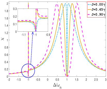
We first demonstrate the optical response of the ONMS by setting i.e., -symmetric ONMS returns to a typical passive system having decay rate and . In Fig. 2, we exhibit the absorption as a function of with and without tunable effective opto-nanomechanical coupling strength. When , sin( become zero and consequently, the effective opto-nanomechanical coupling strength , which leads to a lorentzian curve around as shown in Fig. 2. Thus, opto-nanomechanical coupling between the nanosphere and the cavity field only trap the nanosphere and don’t contribute any additional interference channel. However, when sin(, a nonzero effective opto-nanomechanical coupling strength appears which leads to an NMIT window as shown by the dot-dashed line in Fig. 2. Specifically, there exist two dips which appears around in the presence of , at the probe frequency. This is due to the fact that in ONMS, the nanosphere’s damping rate is notably small (see the Eq. 11) so that the obtained amplitude of the output spectra has the minimal values when (i.e., ), which corresponds to strongest opto-nanomechanical coupling and ONMS system, in this situation, exhibits the normal mode splitting. Hence, effective opto-nanomechanical coupling strength gives rise to symmetric structure, quantified by a NMIT window and two sideband absorption peaks around .
Another fascinating observation is that when we consider the active cavity has neither loss nor gain. To observe the influence of such active cavity, with no loss/gain, on the absorption, we have plotted the absorption spectrum as a function of for different hoping factor in fig. 3. Interestingly, in this situation, we not only obtained NMIT around but also an additional absorption profile appears around . In this case, ONMS still behaves as a passive system because one cavity has neither loss nor gain and the other is lossy.
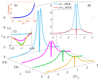
Next, we plot the absorption spectrum as a function of and the photon hoping strength . When , there exists two paths for the generation of photon at the probe frequency in the output field. One is anti-Stokes scattering from the pump field and the other is the probe field itself. The ONMS, in this situation, reduces to typical passive system and there is transparency window at . However, when the photon hoping strength is not zero, i.e., , there exists an additional rout in addition to two previous routs. The additional rout is week probe field passive cavity active cavity passive cavity output. These three routs are responsible for the enhancement of absorption spectra in the output. One can see that only the strength of the absorption peaks (as shown by the inset (A) of Fig. 4.) but also the width of the NMIT window gets broadened with the strengthening as shown in Fig. 4. The inset (B) and (C), in Fig. 4., represent the absorption spectrum around and , respectively. In addition, we also plot the absorption profile when (solid blue line) and (dot-dashed red line), in inset (B) of Fig. 4. It is worth noting that the NMIT spectrum exists for both active-passive case and passive-passive case as shown in the inset (B), in Fig. 4. In addition, the absorption peaks are considerably higher for passive-passive compared to that of active-passive ONMS.
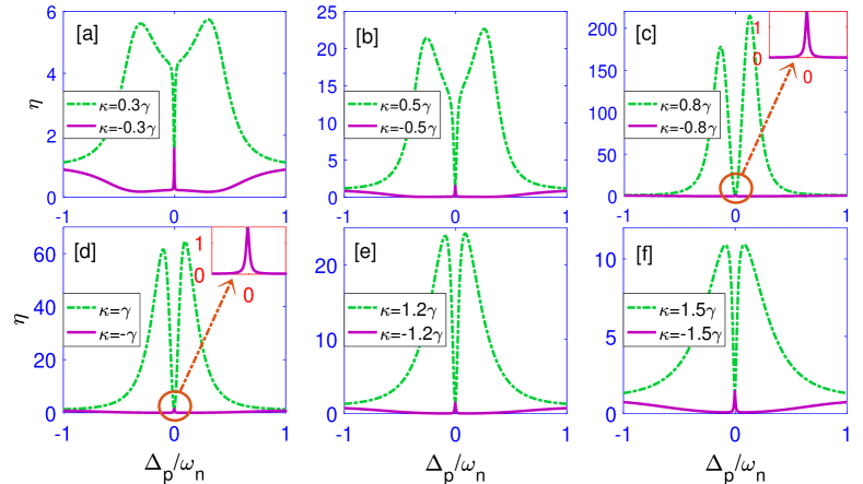
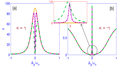
Gain dependence of the optical transmission. For various values of the gain, we depict the transmission as a function of in Figure 5. It is noteworthy that for , the transmission at is very much small as compared to , therefore, we focus our discussion for the prob response around . Fig. 5 illustrates how affects the optical transmission rate. In case of passive-active ONMS, as increases, the heights of the sideband peaks enhances until , where maximum transmission at sidebands occurs. While in case of passive-passive, both sideband peaks are suppressed when the gain is increased further. This is because, if , the system remains in the -symmetry phase; if , on the other hand, the system transits to the -symmetry-broken phase. Owing to the fact that in the -symmetry phase, the criterion can always be satisfied. Nevertheless, if the system is in the -symmetry-broken phase, is not always satisfied . Thus, by adjusting the gain in the active cavity, one can modulate the ONMS to transit from the NMIT to inverted NMIT. Thus, for , the ONMS stays in the -symmetric phase for , but for , the ONMS shifts to the broken- phase. Increasing the gain value above the phase transition value at , the cavity field intensity in the passive cavity is notably reduced which weaken the strength of the ONMS interactions and therefore the value of the transmission. It has a striking resemblance to a previous experiment with two coupled resonators, which demonstrated that lowering (raising) the loss of one resonator below (above) a critical threshold decreases (increases) the other resonator’s intracavity field strength, suppressing (enhancing) transmission BPNG . It’s crucial to remember that increasing (decreasing) gain and decreasing (increasing) loss are similar. Hence, we conclude that the active NMIT in the -regime can be considered as an analog of the optical inverted-EIT OTTM .
Opto-nanomechanical coupling dependence of the optical transmission. It is important to observe the effect of opto-nanomechanical coupling strength on the transmission rate. Since, opto-nanomechanical coupling strength is the product of opto-nanomechanical coupling coefficient and the steady-state value of the cavity field, which depends upon the input laser field with amplitude , so any variation of , through the power of input laser field or through the factor sin directly effects the effective optonanocal coupling strength. Therefore, to investigate the effect of opto-nanomechanical coupling on the transmission rate, we have plotted the transmission rate as a function of for different opto-nanomechanical coupling strengths by varying opto-nanomechanical coupling coefficient via sin. For the passive-active ONMS, increasing the opto-nanomechanical coupling leads to a notable decrease of the sideband amplifications . Furthermore, for the passive-passive ONMS, the width and the transmission rate around increase with increasing opto-nanomechanical coupling (see Fig. 7(b)).
IV CONCLUSIONS
In this paper, we considered a -symmetric two cavity system and studied the tunable optical response of the ONMS, containing a levitating nanosphere inside a passive cavity. ONMS system exhibits NMIT even in a situation with no loss/gain in the active cavity. We also observe an additional absorption profile in this case. Furthermore, the absorption profile notably enhances as the hoping strength between the active and passive cavity increases. Next, for balanced gain/loss case (i.e., ), height as well as the width of the NMIT window increase with increasing hoping factor . We found that the transmission spectrum depends on various system parameters, like, gain-to-loss ratio, detuning, hoping factor and the coupling between the nanosphere and right mirror of passive cavity. An interesting feature is the optical response due to opto-nanomechanical coupling in -symmetric and broken -symmetric regimes has been discussed. Our results show that the presence of nanosphere in the passive-passive cavity enhances the width and transmission rate of NMIT window in passive-passive regime and in passive-active regime, a notable decrease of sideband amplification has been observed. In the end, we assert that this study may find some applications in controlling light propagation and optical switching.
References
- (1) C. M. Bender and S. Boettcher, ”Real Spectra in non-Hermitian Hamiltonians having symmetry”, Phys. Rev. Lett. 80, 5243 (1998).
- (2) C. M. Bender, M. Gianfreda, S. K. Ozdemir, B. Peng and L. Yang, ”Twofold transition in symmetric coupled oscillators”, Phys. Rev. A 88, 062111 (2013).
- (3) B Peng, S. K. Özdemir, F. Lei et al., Parity-time symmetric whispering-gallery microcavities Nat. Phys. 10, 394 (2014).
- (4) R. Driben, B. A. Malomedu. Stability of solitons in parity-time-symmetric couplers. Opt. Lett. 36, 4323-4325 (2011).
- (5) F. Nazari et al. Optical isolation via -symmetric nonlinear Fano resonances. Opt. Express 22, 9574 (2014).
- (6) J. Li, R. Yu, Y. Wu. Proposal for enhanced photon blockade in parity-time-symmetric coupled microcavities. Phys. Rev. A 92, 053837 (2015).
- (7) X. Y. Lü, H. Jing, J. Y. Ma, Y. Wu. -symmetry-breaking chaos in optomechanics. Phys. Rev. Lett. 114, 253601 (2015).
- (8) J. Li, X. Zhan, C. Ding, D. Zhang, Y. Wu. Enhanced nonlinear optics in coupled optical microcavities with an unbroken and broken parity-time symmetry. Phys. Rev. A 92, 043830 (2015).
- (9) S. K. Gupta, A. K. Sarma. Peregrine rogue wave dynamics in the continuous nonlinear Schrödinger system with parity-time symmetric Kerr nonlinearity. Commun. Nonlinear Sci.Numer. Simulat. 36, 141-147 (2016).
- (10) B. Peng et al. Loss-induced suppression and revival of lasing. Science 346, 328-332 (2014).
- (11) A. Regensburger et al. Parity-time synthetic photonic lattices. Nature 488, 167-171 (2012).
- (12) L. Feng et al. Nonreciprocal light propagation in a silicon photonic circuit Science 333, 729-733 (2011).
- (13) L. Chang et al. Parity-time symmetry and variable optical isolation in active-passive-coupled microresonators. Nat. Photon. 8, 524-529 (2014).
- (14) G. S. Agarwall and S. Huang. Phys. Rev. A 81 041803 (2010).
- (15) Sohail, A., Zhang, Y., Zhang, J., Yu, C.S.: Optomechanically induced transparency in multi-cavity optomechanical system with and without one two-level atom. Sci. Rep. 6, 28830 (2016)
- (16) Sohail, A., Zhang, Y., Usman, M., Yu, C.S. Controllable optomechanically induced transparency in coupled optomechanical systems. Eur. Phys. J. D 71, 103 (2017)
- (17) Y. Xiao, Y. F. Yu, Z. M. Zhang. Controllable optomechanically induced transparency and ponderomotive squeezing in an optomechanical system assisted by an atomic ensemble. Opt. Express 22, 17979 (2014).
- (18) Y. Turek, Y. Li, C. P. Sun.Electromagnetically-induced-transparencyClike phenomenon with two atomic ensembles in a cavity. Phys. Rev. A 88, 053827(2013).
- (19) Y. Han, J. Cheng, L. Zhou. Electromagnetically induced transparency in a cavity optomechanical system with an atomic medium. J. Phys. B. At. Mol. Opt. Phys. 44, 165505 (2011).
- (20) Y. Chang, T. Shi, Y. X Liu, C. P. Sun, F. Nori. Multistability of electromagnetically induced transparency in atom-assisted optomechanical cavities. Phys. Rev. A 83, 063826 (2011).
- (21) Brennecke, F., Ritter, S., Donner, T., Esslinger, T.: Cavity optomechanics with a Bose-Einstein condensate Science 322, 235 (2008)
- (22) Ritsch, H. et al.: Cold atoms in cavity-generated dynamical optical potentials. Rev. Mod. Phys. 85, 553 (2013)
- (23) Yasir, K.A., Ayub, M., Saif, F.: Exponential localization of moving-end mirror in optomechanical system. J. Mod. Opt. 61, 1318 (2014)
- (24) Sohail, A., Ahmed, R., Peng, J. X., Shahzad, A. Singh, S. K. Enhanced entanglement via magnon squeezing in a two-cavity magnomechanical system. JOSA B 40(5), 1359 (2023).
- (25) Sohail, A., Qasymeh, M., Eleuch, H. Entanglement and quantum steering in a hybrid quadpartite system. Phys. Rev. Applied 20 054062 (2023).
- (26) A. Sohail, A. Hassan, R. Ahmed, and C. S. Yu, Generation of enhanced entanglement of directly and indirectly coupled modes in a two cavity magnomechanical system, Quantum Inf. Process. 21, 207 (2022).
- (27) A. Sohail, R. Ahmed, R. Zainab, and C. S. Yu, Enhanced entanglement and quantum steering of directly and indirectly coupled modes in a magnomechanical system, Phys. Scr. 97, 075102 (2022).
- (28) Kaltenbaek, R., Hechenblaikner, G., Kiesel, N., RomeroIsart, O., Schwab, K., Johann, U., Aspelmeyer, M.: Macroscopic quantum resonators. Exp. Astron. 34, 123 (2012)
- (29) Arvanitaki, A., Geraci, A.A.: Detecting high-frequency gravitational waves with optically levitated sensors. Phys. Rev. Lett. 110, 071105 (2013)
- (30) Kiesel, N., Blaser, F., Deli, U., Grass, D., Kaltenbaek, R., Aspelmeyer, M.: Cavity cooling of an optically levitated submicron particle. Proc. Nat. Acad. Sci. 110, 14180 (2013)
- (31) Millen, J., Fonseca, P.Z.G., Mavrogordatos, T., Monteiro, T.S., Barker, P.F.: Cavity Cooling a single charged levitated nanosphere. Phys. Rev. Lett. 114, 123602 (2015)
- (32) Chang, D.E., Regal, C.A., Papp, S.B., Wilson, D.J., Ye, J., Painter, O., Kimble, H.J., Zoller P.: Cavity optomechanics using an optically levitated nanosphere. Proc. Nat. Acad. Sci. 107, 1005 (2010)
- (33) Romero-Isart, O., Pflanzer, A.C., Juan, M.L., Quidant, R., Kiesel, N., Aspelmeyer, M., Cirac, J.I.: Optically levitating dielectrics in the quantum regime: theory and protocols. Phys. Rev. A 83, 013803 (2011).
- (34) Hensinger, W.K., Utami, D.W., Goan, H.S., Schwab, K., Monroe, C., Milburn, G.J.: ion trap transducers for quantum electromechanical oscillators. Phys. Rev. A 72(R), 041405 (2005)
- (35) Nie, W., Chen, A., Lan, Y.: Optical-response properties in levitated optomechanical systems beyond the low-excitation limit. Phys. Rev. A 93, 023841 (2016)
- (36) Amjad Sohail , Rizwan Ahmed, Chang Shui Yu and Tariq Munir. Enhanced entanglement induced by Coulomb interaction in coupled optomechanical systems. Phys. Scr. 95 035108 (2020).
- (37) Amjad Sohail, Rizwan Ahmed, Chang shui Yu, Tariq Munir and Fakhar-e-Alam. Tunable optical response of an optomechanical system with two mechanically driven resonators. Phys. Scr. 95 045105 (2020).
- (38) Gröblacher, S., Hammerer, K., Vanner, M., Aspelmeyer, M.: Observation of strong coupling between a micromechanical resonator and an optical cavity field. Nature (London) 460, 724 (2009)
- (39) Nie, W., Lan, Y., Li, Y.: Zhu S.:Dynamics of a levitated nanosphere by optomechanical coupling and Casimir interaction. Phys. Rev. A 88, 063849 (2013)
- (40) D. F. Wall, G. J. Milburn. Quantum Optics. Springer, Berlin (1994)
- (41) H. Jing, et al. Scientific Reports, 5 9663 (2016).
- (42) Amjad Sohail, Rizwan Ahmed, Jia-Xin Peng, Tariq Munir, Aamir Shahzad, S. K. Singh, Marcos Csar de Oliveira.:Controllable Fano-type optical response and four-wave mixing via magnetoelastic coupling in an opto-magnomechanical system. J. Appl. Phys. 133, 154401 (2023).
- (43) Oishi, T. and Tomita, M. Inverted coupled-resonator-induced transparency. Phys. Rev. A 88, 013813 (2013)