Lagrangian Covector Fluid with Free Surface
Abstract.
This paper introduces a novel Lagrangian fluid solver based on covector flow maps. We aim to address the challenges of establishing a robust flow-map solver for incompressible fluids under complex boundary conditions. Our key idea is to use particle trajectories to establish precise flow maps and tailor path integrals of physical quantities along these trajectories to reformulate the Poisson problem during the projection step. We devise a decoupling mechanism based on path-integral identities from flow-map theory. This mechanism integrates long-range flow maps for the main fluid body into a short-range projection framework, ensuring a robust treatment of free boundaries. We show that our method can effectively transform a long-range projection problem with integral boundaries into a Poisson problem with standard boundary conditions — specifically, zero Dirichlet on the free surface and zero Neumann on solid boundaries. This transformation significantly enhances robustness and accuracy, extending the applicability of flow-map methods to complex free-surface problems.
1. Introduction
Flow map methods have garnered increasing interest in both computational physics and computer graphics communities in recent years, as evidenced by the emergence of covector/impulse-based (Nabizadeh et al., 2022; Deng et al., 2023) and vorticity-based (Mercier et al., 2020; Yin et al., 2021, 2023) solvers that are known for their exceptional preservation of vortical structures. The key to developing a flow-map method is constructing an efficient and accurate representation that maps any given point from the initial to the current frame (and vice versa if a bi-directional mapping process is necessary). This flow map, or the relationship between the two endpoints of every mapping trajectory sample, was previously realized by advecting the spatial coordinates (Hachisuka, 2005; Sato et al., 2017, 2018; Tessendorf, 2015; Deng et al., 2023), with improved accuracy later achieved by tracing particles backward over a recorded spatiotemporal velocity field, both of which were implemented in a fixed, Eulerian domain.
One of the main challenges in the impulse/covector fluid models with their flow-map-based implementations is addressing free-surface boundaries. Existing approaches struggle to simulate free-surface fluids due to inherent difficulties with free-surface boundary conditions that are impractical to manage using traditional numerical solvers. In standard free-surface solvers built on velocity space, fluid incompressibility is enforced by solving a Poisson problem with zero Dirichlet boundary conditions on the free surface (assuming zero air pressure) and appropriate Neumann boundary conditions on solid boundaries. In contrast, the free-surface boundary conditions for a covector flow map model pose greater challenges. This difficulty arises from the complexity of calculating the kinetic energy integral on the free boundary over the entire flow map interval.
In typical liquid simulation scenarios in computer graphics, the fluid surface undergoes extensive geometric and topological transitions over time. Consequently, a fluid particle may appear on the surface at a certain instant and then merge into the fluid body later. This dynamics makes it impractical to track these particles’ statuses consistently and determine whether they are on the free surface at any given time over a high-dimensional spatiotemporal space. However, the accuracy of the boundary condition depends on the path integral of all particles currently on the free surface over the entire flow-map period. Due to these challenges with traditional numerical solutions, the covector/impulse frameworks and their flow-map implementation are confined to solving fluid without a free surface and can produce smoke animations only.
This paper makes the first step toward addressing the free-surface boundary challenges for covector flow-map methods. We attack the problem from the Lagrangian perspective by treating each flow-map sample as a Lagrangian particle trajectory. Under this Lagrangian view, we proposed a novel mathematical framework based on the path integral identities in flow-map theory to decouple the mapping and projection steps in a conventional covector flow-map algorithm. Our key idea is to leverage these mathematical identities to flexibly control the integral intervals for different physical quantities along each Lagrangian path, and then transform the boundary conditions from the long-range integral (through all flow map time steps) to a short-range integral (within a single time step), and eventually to a standard zero Dirichlet boundary to fit into the existing Poisson solver. By doing so, we can decouple the long-range map for velocity, which serves as the enabling mechanism for the vortical expressiveness of flow-map methods, and the pressure projection step, which is fundamental for simulating incompressible flow, without any model degeneration or artificial numerical blending.
Our proposed Lagrangian covector solver comprises three components: a Lagrangian model for long-range flow maps and path integrals, a reformulated Poisson solver designed for handling complex boundaries, and a Voronoi-based numerical implementation. These components synergistically establish a particle-based framework that facilitates integral-flexible flow maps for the first covector solver capable of handling free surfaces.
We summarize our main contributions as follows:
-
•
We proposed a novel Lagrangian flow map model characterizing the path integral form of covector fluid.
-
•
We proposed a novel mechanism to incorporate long-range flow maps into a short-range projection step and reformulated it into a standard Poisson problem.
-
•
We proposed the first free-surface covector fluid model based on a Voronoi implementation.
2. Related Work
Particle-based fluid simulation
(De Goes et al., 2015) introduced power particles to simulate incompressible fluids. Their geometrically inspired method offers precise pressure solving and an even distribution of particles by describing the fluid motion as a series of well-shaped power diagrams. (Zhai et al., 2018) accelerated the construction of power diagrams on GPUs, adopting ghost particles for fluid-air interactions, while (Lévy, 2022) introduced a more precise technique to calculate free-surface interactions, framing it as an optimal transport problem.
Flow-map methods
The method of characteristic mapping (MCM) of Wiggert and Wylie (1976) was first introduced to the graphics community by Tessendorf and Pelfrey (2011). Due to its superiority in dealing with numerical dissipation through long-range mapping, some methods (Hachisuka, 2005; Sato et al., 2017, 2018; Tessendorf, 2015) trade off computational cost for better accuracy utilizing virtual particles for tracking the mapping. Subsequently, Nabizadeh et al. (2022) combined this with an impulse fluid model (Cortez, 1996) and Qu et al. (2019) developed a bidirectional mapping to prevent dissipation better. Deng et al. (2023) stores intermediate velocity fields using a neural network for storage compression. We track such mapping directly with particles. Compared to previous flow map methods (e.g., (Sato et al., 2017)), our method relies on calculating path integrals on particles directly without any backtrace step, eliminating any extra velocity buffer.
Gauge-based fluid
The concept of the impulse variable was initially introduced in (Buttke, 1992), reformulating the incompressible Navier-Stokes Equation with a gauge variable and transformation (Oseledets, 1989; Roberts, 1972; Buttke, 1993). Various gauges have been proposed for applications like boundary treatment, numerical stability, and turbulence simulation (Buttke, 1993; Buttke and Chorin, 1993; Weinan and Liu, 2003; Cortez, 1996; Summers, 2000). Saye (2016) and Saye (2017) employed a different gauge for interfacial discontinuity issues. In the graphics community, researchers like Feng et al. (2022), Xiong et al. (2022), Yang et al. (2021), and Nabizadeh et al. (2022) have explored this area, though facing challenges with accurate advection. Flow maps, as shown in (Deng et al., 2023), are effective for advecting such variables, and this method has been adapted to particles in our research.
3. Mathematical Foundation
| \hlineB 3 Notation | Type | Definition |
| \hlineB 2.5 | scalar | Current time |
| \hlineB 1 | scalar | Initial time |
| \hlineB 1 | scalar | One time step before the current time |
| \hlineB 1 | vector | Forward flow map from time to |
| \hlineB 1 | vector | Backward flow map from time to |
| \hlineB 1 | matrix | Jacobian of forward flow map |
| \hlineB 1 | matrix | Jacobian of backward flow map |
| \hlineB 1 | scalar | Pressure at time |
| \hlineB 1 | scalar | Lagrangian pressure calculated at time |
| \hlineB 1 | scalar | Integration of from time to |
| \hlineB 1 | vector | Mapped velocity at time by covector flow map from time |
| \hlineB 1 | vector | Advected velocity at time by particle velocity from time |
| \hlineB 3 |
Flow Maps
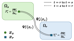
To define the flow map, we start with an initial domain at time and its current domain at time , with . A particle at at time moves to at time by velocity . The relationship between and is defined through two flow map functions, including the forward flow map and the backward flow map , with Jacobians and . These two flow maps satisfy the equations and , where and denote the identity transformations in domains and respectively.
Considering the domain (where ) at any time as a linear vector space, the flow maps and are mappings between these linear spaces. Given a scalar field at time , a scalar field on can be induced via the map (∗ means induction, where a map between fields is induced by a map between domains). This induced scalar field is called the pullback of by the mapping (the pullback by is similar).
Covector Preliminaries
In the domain at any time , regarded as a linear space, we can define tangent spaces and cotangent spaces at any point within . For , the tangent spaces encompass all vectors originating from , while the cotangent space comprises all linear functions (termed cotangent vectors or covectors) defined on . Given an inner product in , any tangent vector induces a covector in , such that for all . Here, denotes the conversion of a tangent vector to a covector, and signifies the reverse conversion. A vector field (or covector field ) is formed by selecting one vector (or one covector ) from each tangent space (or the cotangent space ) at every point . The gradient of a scalar field can be considered as a vector field. Refer to (Crane et al., 2013) for details.
Lie Advection
For any covector field taken from , induces a covector field on as , which is referred to as the pullback of the covector field by . The pullback of at any time satisfies an Lie advection equation:, where is the Lie derivative, and in , it is given by . Therefore if there is a vector field that satisfies this advection equation, at any time , can be described through the pullback of the initial through pullback.
4. Physical Model
Covector Incompressible Fluid
We model incompressible flow using Euler equations by assuming viscosity zero and density one:
| (1) |
with and specifying the fluid velocity and pressure. The first equation describes the momentum conservation, and the second equation specifies incompressibility. According to the covector model proposed in (Nabizadeh et al., 2022), Equation 1 can be reformulated into its covector form as , which can be further written with Lie advection as
| (2) |
where is defined as Lagrangian pressure.
Covector Fluid on Flow Maps
The solution of Equation 2 at includes terms obtained by pulling back the velocity field as a covector through the flow map. This process is illustrated by integrating both sides of Equation 2 from time to , represented as a covector:
| (3) | ||||
with the second line arising from the commutativity between the differential operator (more accurately denoted as “d”) and the pullback operator (Equation 7 in (Nabizadeh et al., 2022)), and commutativity between and the integral sign.
Next, we can convert the covector forms and their pullbacks in Equation 3 into their vector forms as:
| (4) |
which constitutes two main steps to obtain velocity at using a mapping-projection scheme. Initially, the mapping step calculates as the pullback of the velocity field by the flow map. In the projection step, the gradient of is projected from the mapped velocity to enforce incompressibility.
5. Path Integral on Lagrangian Flow Maps
Equation 4 can be written into a path integral form on a Lagrangian trajectory. For a fluid particle with position at any time , the projection term in Equation 4 is the path integral of along its trajectory from time to , which is denoted as
| (5) |
Here the subscript indicates that this quantity is carried by the particle . For the mapping part, is the velocity of particle at time , and we simplify the notation as . Because is determined by the positions of all particles in the flow field at time and , it can be carried on fluid particles, denoted as . We obtain the reformulated Equation 4 as a path integral:
| (6) |
Equation 6 forms the mathematical foundation of our Lagrangian covector fluid model. This equation, in contrast to Equation 4, considers the mapping and projection processes occurring on a particle as it moves along its trajectory in the flow field, which simplifies the formulation by eliminating the need for back-and-forth mappings to identify a Lagrangian point. Thus, we reinterpret the mapping-projection process on a moving particle as follows: (1) calculate the mapped velocity from the initial time as , and (2) remove its irrotational component by subtracting the gradient of the path integral of the Lagrangian pressure .
6. Incompressibility
6.1. Long-Range Mapping, Long-Range Projection
To determine the velocity of a particle at time , we initially consider a straightforward method for solving Equation 6. We present the method as a standard mapping-projection scheme:
-
(1)
(Long-Range Mapping) Calculate the long-range mapped velocity as: ;
-
(2)
(Long-Range Projection) Solving the following Poisson equation to obtain :
(7) where denotes the velocity of the solid boundary, and and denote solid boundary and free surface boundary respectively. Then, we carry out a projection as to ensure satisfies .
Here, is long-range mapped from the initial time and is projected to by a gradient of long-range path integral of pressure from time to . Hence, the Poisson equation we solve in Equation 7 leads to a long-range projection of the rotational component accumulated from time to time . Given these, we refer to this strategy as Long-Range Mapping Long-Range Projection (LMLP).
LMLP has two main issues regarding boundary and performance:
-
(1)
Setting boundary conditions is challenging. Specifically, at the free boundary , to enforce the boundary condition , we define . This implies the necessity of establishing a non-zero Dirichlet boundary condition such that . This condition requires a comprehensive path integral of the kinematic energy across a particle’s trajectory. Although seemingly feasible from a Lagrangian perspective, it is crucial to recognize that this path integral only constitutes a valid Dirichlet boundary under the specific condition that the particle remains on the free surface from time to . However, in practical scenarios, this condition is rarely met due to the dynamic topological changes of the surface over time. In the interval from time to , particles may transition between the interior and the surface, rendering the calculation of this integral impractical.
-
(2)
The performance issue is notable. The term encompasses a substantial divergent component , which includes an integral extending from time to . Attempting to eliminate this component through a single projection results in significant computational expenses, primarily due to the increased number of iterations required for solving the Poisson equation.
6.2. Short-Range Mapping, Short-Range Projection
To address the two issues mentioned above, we devise a short-range approach. By setting the flow map’s start point to be only one timestep before , denoted as , we can calculate the velocity at time with the following two steps:
-
(1)
(Short-Range Mapping) Calculate the mapped velocity:
-
(2)
(Short-Range Projection) Solve the following Poisson equation to obtain :
(8) where is the numerical calculation of one step integration . Then, we conduct the divergence-free projection as .
Given both mapping and projection are limited within a short interval from time to , we refer the scheme as Short-Range Mapping Short-Range Projection (SMSP). It is worth noting that SMSP is akin to the Semi-Lagrangian advection schme, as they both involve computing a one-step mapping. The difference lies in the fact that SMSP employs a mapping form based on the Lie advection equation , whereas Semi-Lagrangian employs a mapping form based on the ordinary advection equation .
SMSP ensures robustness by addressing the two issues above: (1) The Neumann boundary can be set as , namely, , which is robustly calculable (because of only one timestep). (2) The Poisson solve converges fast thanks to the small divergence on its right-hand side. However, SMSP forgoes the advantages associated with employing a long-range flow map for vorticity conservation. Instead, it resolves to a reformulated Euler equation in covector form, accompanied by a one-step particle advection process. This approach results in the loss of the benefits inherent in utilizing a flow map to preserve vorticies.
6.3. Long-Range Mapping, Short-Range Projection
A natural next step is to combine the merits of LMLP and SMSP. However, this is not mathematically intuitive. As shown in Equation 6, the mapping and projection steps require the same time interval for their path integrals.
To address this issue, we observe the following identity:
| (9) |
This identity can be simply proved as and . It establishes a connection between the long-range and short-range mappings, allowing us to express a short-range mapping by adding the gradient of pressure integral to its long-range counterpart. This calculation is numerically robust, because for each particle, is the path integral of the Lagrangian pressure on its trajectory. Substituting Equation 9 into Equation 8, we obtain the following scheme:
-
(1)
(Long-Range Mapping) Calculate mapped velocity by the long-range flow map: ;
-
(2)
Calculate mapped velocity by short-range flow map based on the long-range mapped velocity as:
-
(3)
(Short-Range Projection) Solve the following Poisson equation to obtain :
(10) where is the numerical calculation of one step integration
-
(4)
Update the integral: and project to ensure satisfies .
We name it as Long-Range Mapping Short-Range Projection (LMSP). In LMSP, the in Step (2) is calculated in the previous time step, and this value is updated in Step (4) by to the value in the current time step. This accumulation might lead to a concern that accumulating pressure could potentially lead to the accumulation of numerical errors, thereby diminishing the long-range map’s ability to preserve vorticity when calculating in Step (2). We show this is not an issue. Because is a gradient field, it only affects the divergence component of . Any numerical error accumulated in goes directly into the rotational part , which will be removed after projection.
We further demonstrate this with the following proposition:
Proposition 6.1.
Poission Equation 10 with initial guess is equivalent to Poission Equation 7 with initial guess
Proof:
Substitute Equation 9 into Equation 10, we obtain ], which is equivalent to . Use to substitute , and we get Equation 7. Also, for the initial guess, when , .
7. Adapting to Classical Advection-Projection
In the final movement, we further adapt the LMSP scheme to a classical advection-projection scheme by solving the Poisson equation with standard Neumann and Dirichlet boundary conditions, namely on and on . This modification is motivated by the desire to circumvent any inaccuracies arising from the approximation of for a particle on the surface (due to the lack of sufficient neighboring particles to approximate the Jacobian), which could potentially lead to numerical instabilities during the simulation. We showed an ablation test for this issue in Fig. 11.
We observe the following identity regarding a particle’s velocity on a one-step flow map:
| (11) |
where represents the passively advected velocity on the particle’s trajectory, namely, to move the particle to a new position and keep its velocity as it is, as seen in all traditional particle-based advection schemes. We show a brief proof in the Appendix A.
Combining Equation 9 and Equation 11, we obtain our final advection-projection scheme as:
-
(1)
(Long-Range Mapping) For the interior particles, calculate the long-flow-map mapped velocity: .
-
(2)
For an interior particle, calculate its velocity as the advected velocity expressed with long-flow-map mapped velocity (Eq. 11): .
-
(3)
For a boundary particle (refer to Figure 4), calculate its velocity as the advected velocity: .
-
(4)
(Classical Projection) Solve the classical Poisson equation to obtain :
(12) -
(5)
Update the integral: and do projection for interior part, and for the part near free surface.
We name it as Long-Range Mapping Classical Projection (LMCP). In this scheme, the calculation of the Poisson equation is performed for throughout the entire domain, ensuring the mathematical consistency of the final velocity by the covector flow map and the advected velocity after projection. At the same time, for interior particles, the advected velocity is calculated by with long-range mapping for vorticity preserving. Again, because only the gradient is added to , similar to subsection 6.3, the process of adding to to obtain keeps the long-range flow map’s ability to preserve vorticity.
8. Time Integration
We adopt the LMCP scheme in our simulation and summarize the time integration scheme of our approach in Algorithm 1. We provide further implementation details in the Appendix B.
Input: Initial velocity ; Initial particle positions ; Re-initialization decision strategy ; Near-surface judgment
9. Numerical Implementation
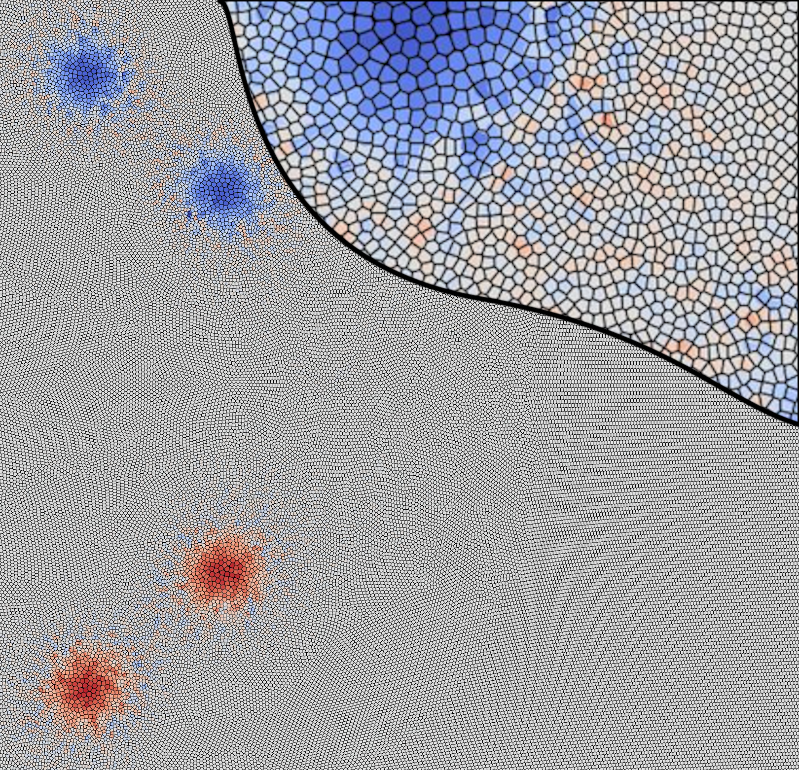
Voronoi-based Discretization
We implemented a Voronoi-based particle method for numerical implementation. In each time step, we generate Voronoi diagrams for all moving particles, with each particle corresponding to a Voronoi cell. We represent the -th particle as , with position . As shown in Fig. 3, the cell corresponding to is denoted , with a volume and centroid . The adjacent facet between two neighboring cells and is denoted as . The facet has the area and the centroid . The distances from and to the facet are respectively denoted as and , while the distance between and is denoted as . According to the properties of Voronoi diagrams, bisects the line connecting and perpendicularly, so and holds.

For each particle , its associated Voronoi cell is used to define a matrix-form discrete gradient operator and divergence operator to calculate the gradient of a scalar quantity and the divergence of a vector quantity carried by particles. The computation of these operators relies on the calculation of the rate of change of the volume induced by particle positions. We use the formula and for calculating as given in (De Goes et al., 2015).
According to (De Goes et al., 2015; Duque, 2023), the matrix-form divergence operator and gradient operator can be defined directly from as , and . The divergence of and the gradient of can be computed using the matrix-form divergence and gradient operators defined as follows:
| (13) | i | |||
where represents the set composed of the cells adjacent to cell .
When solving the Poisson equation for velocity projection, the Laplacian operator is defined as , where is a diagonal matrix composed of all cell volumes . Because the differential operator matrices satisfy , the operator is symmetric and positive semi-definite, allowing the discretized Poisson equation to be solved using the Conjugate Gradient method, where represents the velocity before the divergence projection.
Boundary
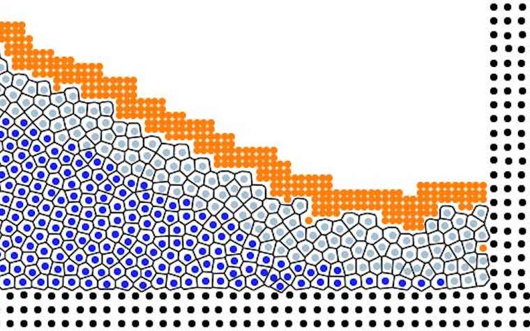
Similar to (De Goes et al., 2015), we represent the solid boundary using solid particles and sample air particles near the free surface, utilizing the ghost particle method from (Schechter and Bridson, 2012) (see Fig. 4). Solid particles and air particles are used for clipping the Voronoi diagrams calculated for fluid particles and setting boundary conditions, as proposed in (De Goes et al., 2015).
Others
For gravity, we accumulate the integration of gravity along the particle trajectory and add it to the mapped velocity before projection: for interior part and add gravity directly to advected velocity near the free surface. To make particle distribution more uniform, like in (De Goes et al., 2015), at the end of each time step, we put particles to the centroid of their corresponding Voronoi cell .
10. Results and Discussion
Validation
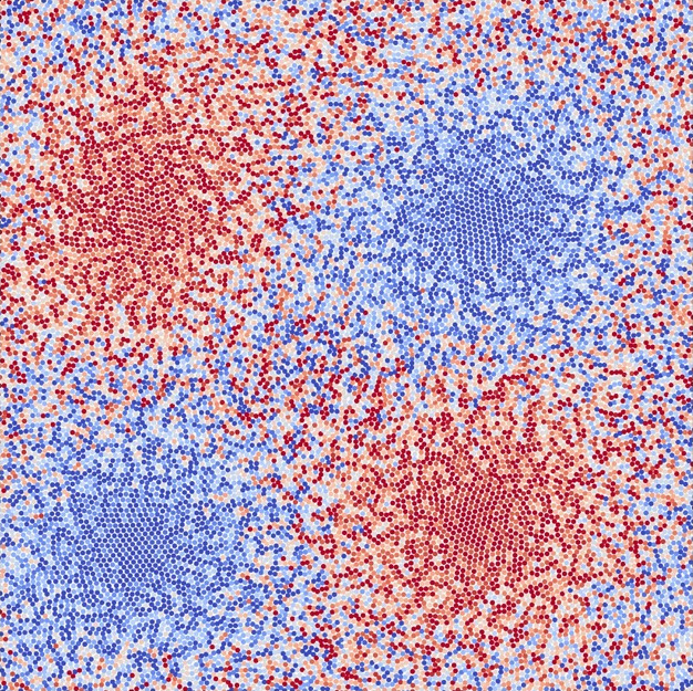
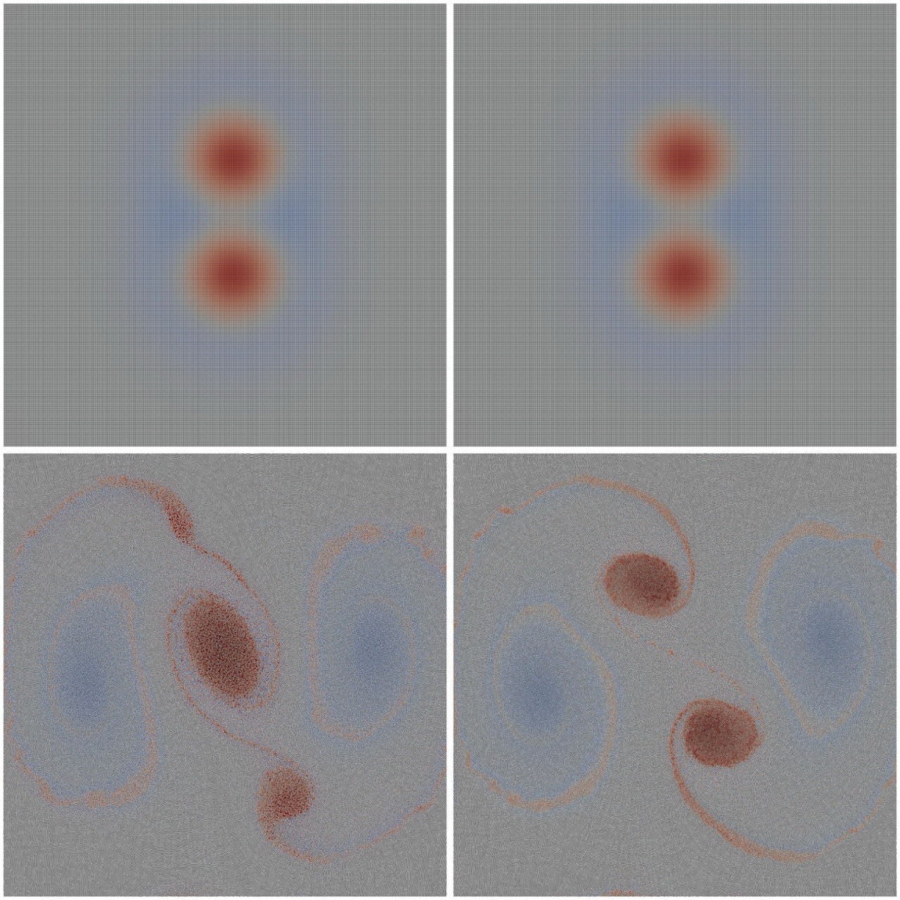
We demonstrate the effectiveness of our method by performing four benchmark experiments against the power particle method (PPM) (De Goes et al., 2015)111For simplicity, we implement a Voronoi diagram instead of the power diagram without affecting the ability to preserve vortex for both our methods and PPM., which shares implementation-wise similarities given its geometric data structure. We observe slower energy dissipation rates, less vorticity noise, and better preservation of vortical structures. We color each 2D particle blue (lower/negative values) through gray to red (higher/positive values), based on a linear curve corresponding to its vorticity magnitude.
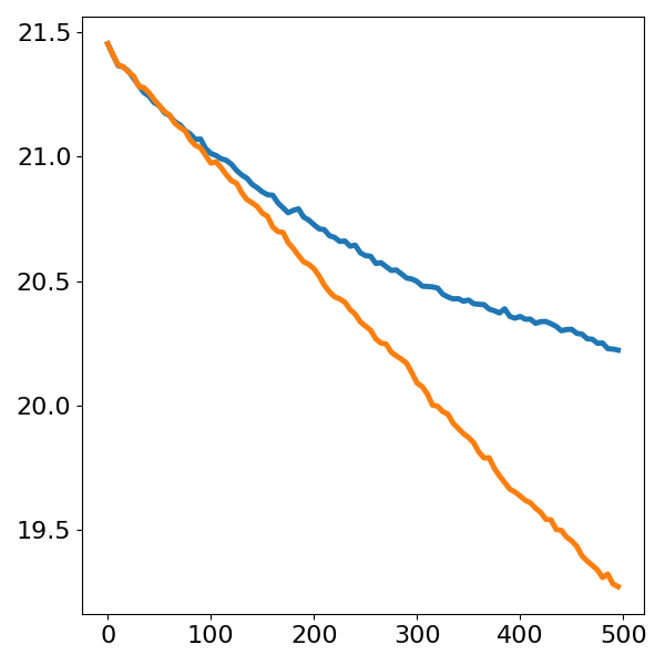
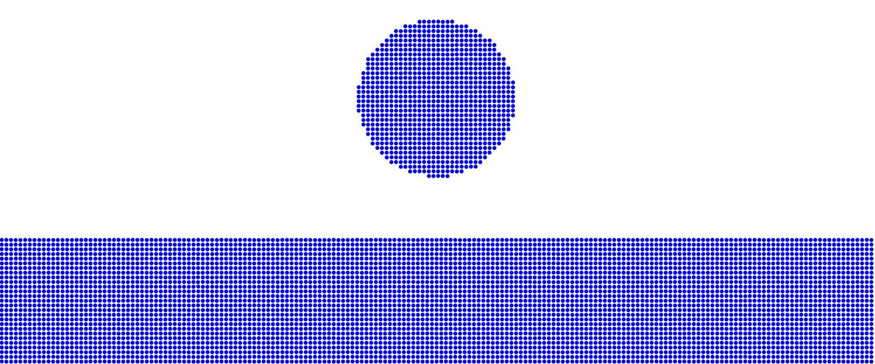
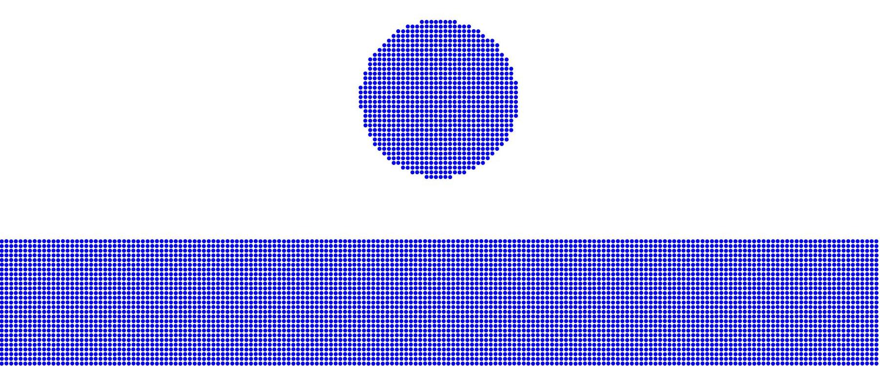
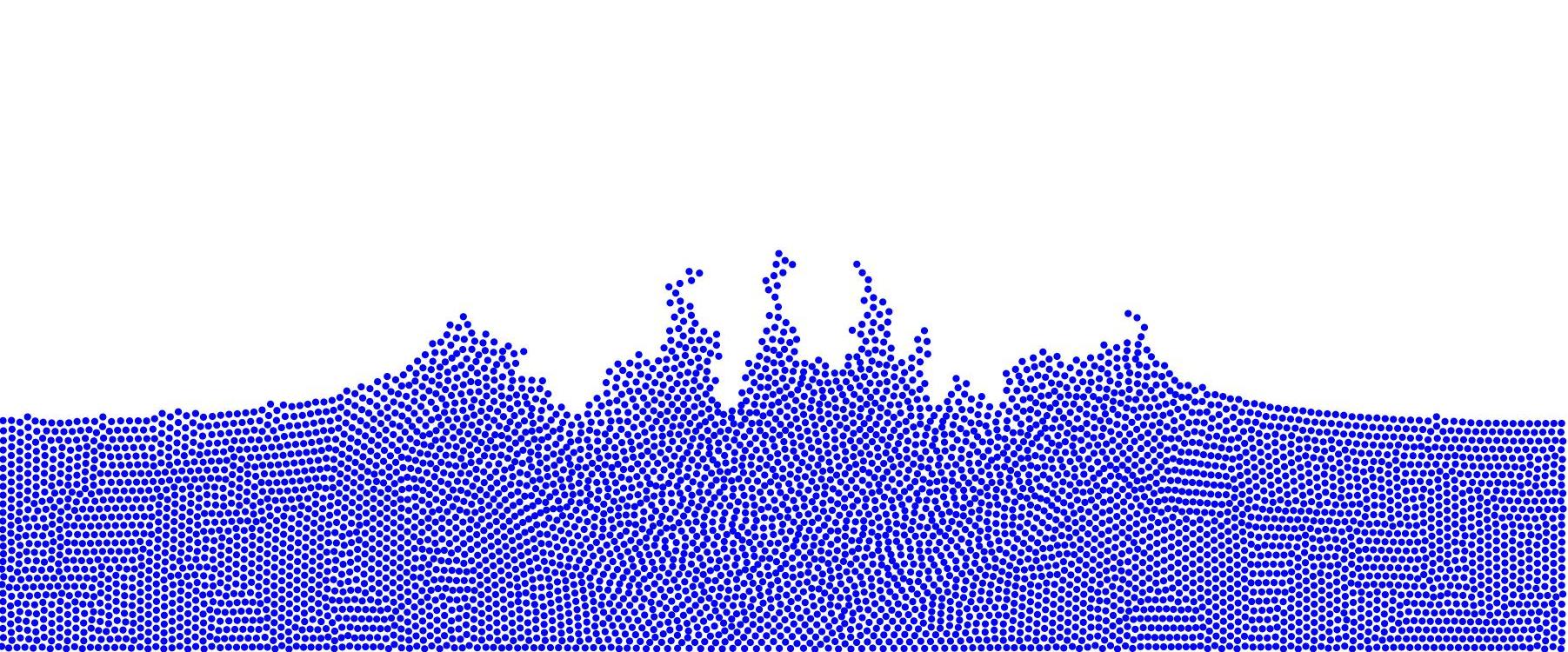
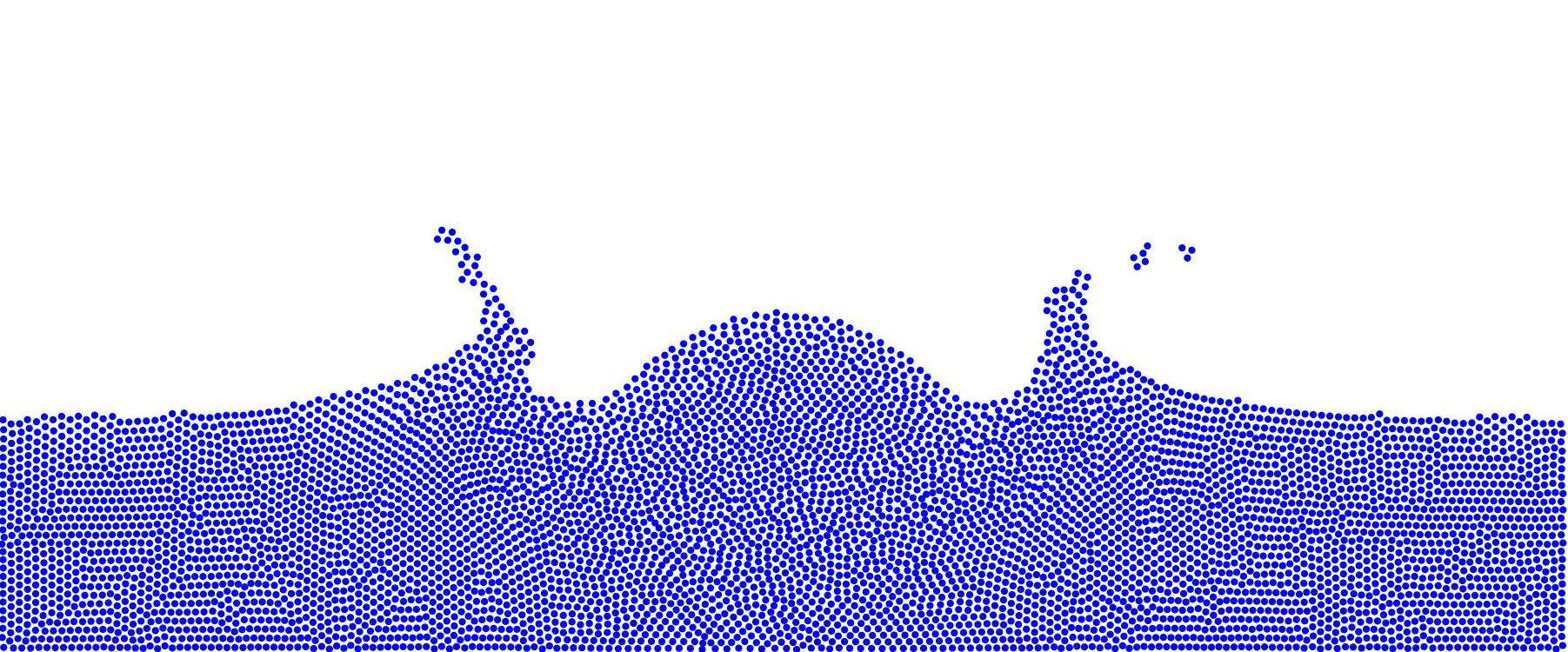
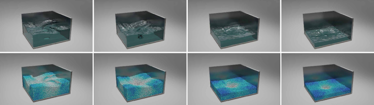
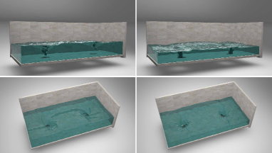
(1) Leapfrog. We initialize two negative and two positive vortex rings, letting the four vortices move forward by the velocity field generated by their influence on each other. The rate of energy dissipation directly relates to the number of cycles they move forward before merging. As illustrated in Fig. 7, our method shows a better preservation of the vortical structures than PPM; vortices simulated with our method stay separated at the point where the vortices in the PPM simulation already merged. (2) Taylor Vortices. We benchmark our method by simulating two Taylor vortices placed apart from each other (Fig. 17). Their velocity field is given by , where we use and , and denotes the distance from to the vortex center.Using our method, we observe the vortices staying separate, whereas using PPM, they merge at the center. (3) Taylor-Green Vortices. Fig. 11 shows a simulation started with a symmetric divergence-free velocity field. The fluid is expected to maintain symmetry along the two axes in 2D while rotating. We observe our method producing less noise in terms of vorticity magnitude carried by the particles as compared to PPM (Fig. 11a-b), with our method presenting a far better energy dissipation curve (Fig. 11c). (4) 3D Dam Break. In Fig. 9, we validate our method with the classical 3D benchmark case for verification of solid boundary and free surface flow handling.
Ablation Study
We illustrate (1) the robustness of our LMCP scheme in handling free surface boundary and (2) the subtraction of accumulated pressure gradient significantly accelerating the convergence rate. Fig. 11 illustrates a robust interface achieved using our scheme, in contrast to instabilities that occur without it. Fig. 7 shows that the subtraction of the accumulated pressure gradient can accelerate the convergence of the Poisson equation solver.
Examples
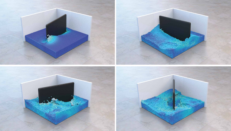
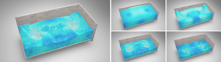
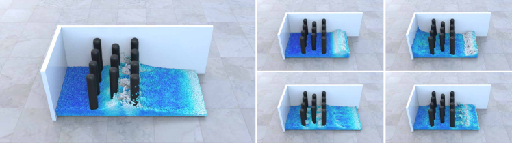
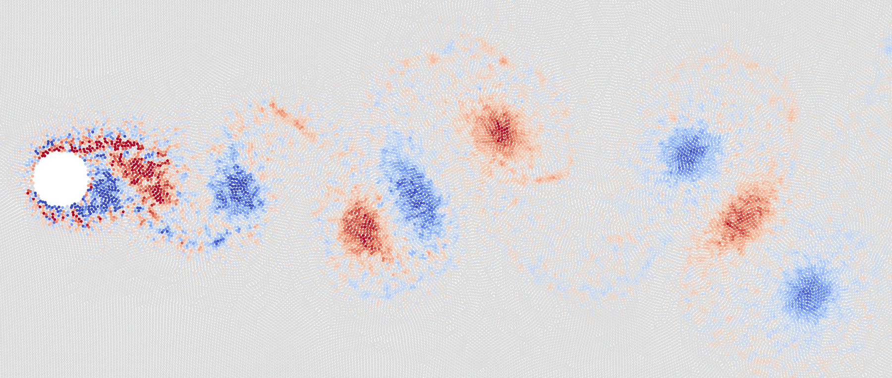
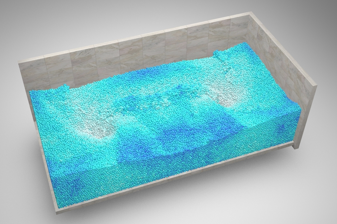
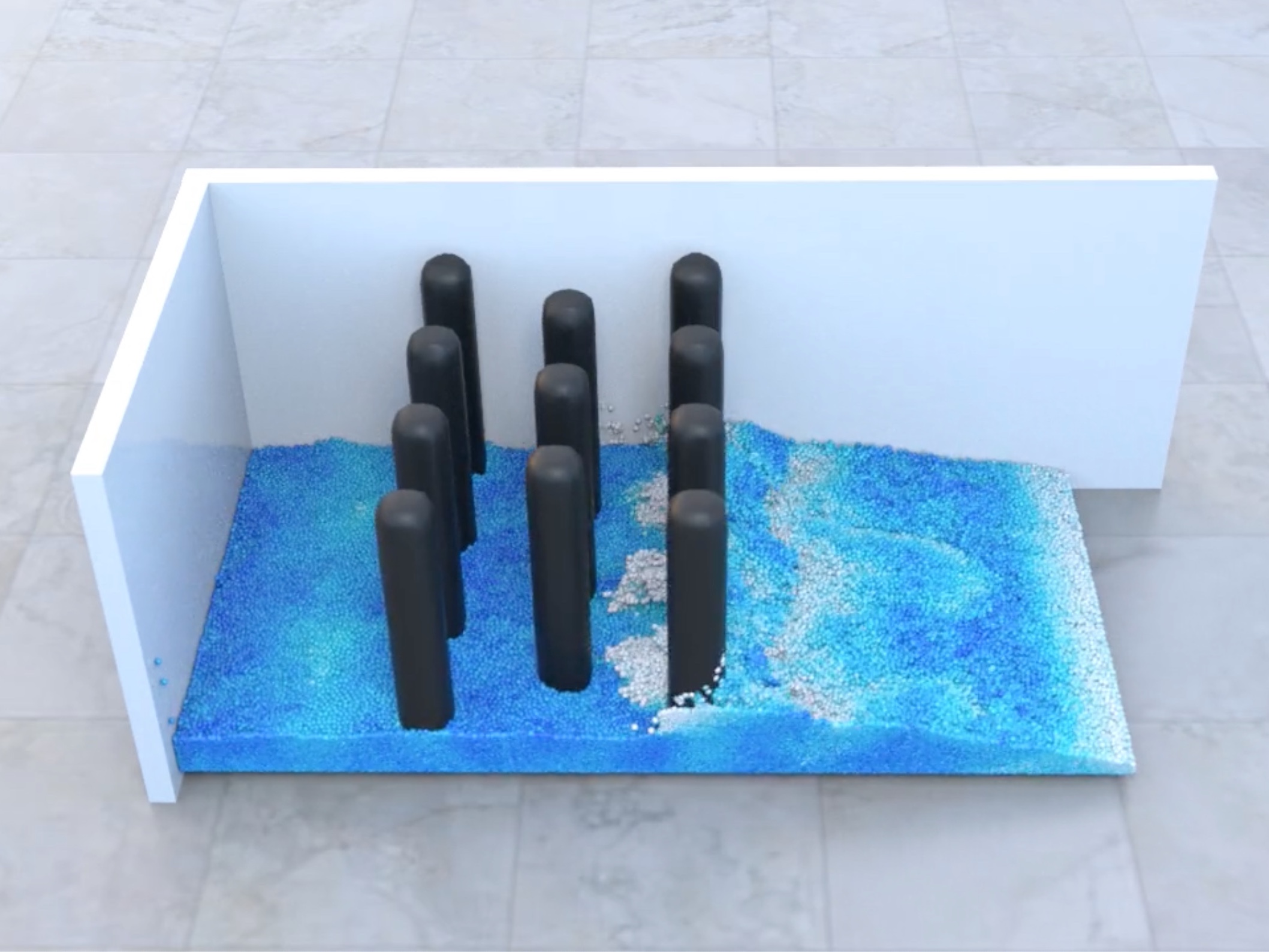
We show additional 2D and 3D examples to demonstrate the robustness and correctness of our method. We use Taichi (Hu et al., 2019) for our implementation, and experiments are run on Tesla V100 GPUs. We use at most particles in all experiments to represent fluid, air, and solids. Voronoi diagrams are created using Scipy (Virtanen et al., 2020) and Qhull (Barber et al., 1996). Kármán Vortex Street. Fig. 17 shows alternating vortices forming downstream from a blunt object caused by the unsteady separation of the fluid. 2D Moving and Rotating Board Fig. 5 shows an object exhibiting flapping motion by traversing the rectangular domain from left to right, and back while generating vortices in its wake. 3D Single & Double Sink In these examples, we illustrate our method’s ability for accurate vorticity perservation combining with free-surface treatment. For single vortex example, we place an initial vorticity field at the center of the tank. A hole is opened as the sink for the tank and water drains out through the hole. Similar settings are adopted for two sink but the sinks have opposite direction of rotation in order to create interesting surface motion. We can observe spiral patterns on the surface in both examples. Results are shown in Fig. 12, Fig. 17 and Fig. 13 3D Rotating Board As illustrated in Fig. 9, a board is placed at the center of the scene and set to rotate at a constant speed. We show our method can handle drastic free-surface change and we deal moving solid boundaries in a robust and effective way. Splashes and detailed water surfaces can be observed. 3D Wave Generator. In this example, we demonstrate the scenario of waves crashing against several pillars. We observe the dynamic water flow behind the pillars and the interaction between the waves. We show particle view for this example in Fig. 14.
CFL
In all of our examples, we set the CFL number to due to constraints imposed by the Voronoi particles. Larger CFL numbers could lead to drastic changes in the neighbors of particles, potentially causing stability issues. Grid-based methods (Nabizadeh et al., 2022) do not encounter these issues.
| Average Time Cost per Substep | ||
| Scene name | Particles | Total (Voronoi) |
| 2D Leapfrog | 480k | 12.5s (8.8s) |
| 2D Taylor Vortices | 360k | 9.8s (6.4s) |
| 2D Taylor-Green Vortices | 156k | 5.96s (2.7s) |
| 3D Dam Break | 211k | 20.9s (18.12s) |
| 2D Kármán Vortex Street | 381k | 9.56s (6.74s) |
| 2D Moving and Rotating Board | 150k | 5.92s (2.66s) |
| 3D Sink | 180k | 29s (25.7s) |
| 3D Rotating Board | 150k | 5.9s (2.6s) |
| 3D Wave Generator | 403k | 35s (32.84s) |
11. Limitations and Future Work
In summary, this paper presents a novel Lagrangian approach to establishing covector flow maps under complex boundary conditions. The developed decoupling mechanism, rooted in flow-map theory, effectively combines long-range flow maps with short-range (and classical) projections, ensuring robust handling of free boundaries.
A significant limitation of our approach lies in its exclusive treatment of inviscid flows. Addressing viscous flows, as well as other interfacial phenomena, represents a promising direction for future research. Currently, the speed of our fluid simulation code is constrained by the single-threaded Qhull algorithm used for generating Voronoi cells in each frame. We plan to investigate more efficient schemes for solving incompressibility on particles. In our future work, we aim to delve further into flow-map theories within a weakly compressible framework, enhancing meshfree Lagrangian methods such as SPH. Additionally, we are interested in applying our decoupled mapping-projection scheme to other free-surface problems, including levelset-based and particle-grid methods.
Acknowledgements.
We acknowledge NSF IIS #2313075, ECCS #2318814, CAREER #2420319, IIS #2106733, OISE #2153560, and CNS #1919647 for funding support. We credit the Houdini education license for the production of the video animations.Appendix A Proof of Eq. 11
Proof:
Consider one step advection from time to and we have . Thus the Jacobian can be calculated as , where denotes identity matrix. Thus . In the particle method, . Due to , we have .
Appendix B Implementation Details of Algo. 1
Reinitialization. We employ a simple reinitialization decision strategy triggered every substeps ( in our implementation).
Boundary particle checking. We employ the following strategy to obtain the boundary particle set : At the initial time , set the flag to False; at each step, check if the particle is in the layers of particles near the free surface at current time . If it is, we update the flag to True; returns the value of .( in our implementation).
References
- (1)
- Barber et al. (1996) C.B. Barber, D.P. Dobkin, and H.T. Huhdanpaa. 1996. The Quickhull algorithm for convex hulls. ACM Transactions on Mathematical Software (TOMS) 22, 4 (Dec 1996), 469–483. http://www.qhull.org
- Buttke (1992) TF Buttke. 1992. Lagrangian numerical methods which preserve the Hamiltonian structure of incompressible fluid flow. (1992).
- Buttke (1993) Tomas F Buttke. 1993. Velicity methods: Lagrangian numerical methods which preserve the Hamiltonian structure of incompressible fluid flow. In Vortex flows and related numerical methods. Springer, 39–57.
- Buttke and Chorin (1993) Thomas F Buttke and Alexandre J Chorin. 1993. Turbulence calculations in magnetization variables. Applied numerical mathematics 12, 1-3 (1993), 47–54.
- Cortez (1996) Ricardo Cortez. 1996. An impulse-based approximation of fluid motion due to boundary forces. J. Comput. Phys. 123, 2 (1996), 341–353.
- Crane et al. (2013) Keenan Crane, Fernando de Goes, Mathieu Desbrun, and Peter Schröder. 2013. Digital geometry processing with discrete exterior calculus. In ACM SIGGRAPH 2013 Courses (Anaheim, California) (SIGGRAPH ’13). Association for Computing Machinery, New York, NY, USA, Article 7, 126 pages. https://doi.org/10.1145/2504435.2504442
- De Goes et al. (2015) Fernando De Goes, Corentin Wallez, Jin Huang, Dmitry Pavlov, and Mathieu Desbrun. 2015. Power particles: an incompressible fluid solver based on power diagrams. ACM Trans. Graph. 34, 4 (2015), 50–1.
- Deng et al. (2023) Yitong Deng, Hong-Xing Yu, Diyang Zhang, Jiajun Wu, and Bo Zhu. 2023. Fluid Simulation on Neural Flow Maps. ACM Transactions on Graphics (TOG) 42, 6 (2023), 1–21.
- Duque (2023) Daniel Duque. 2023. A unified derivation of Voronoi, power, and finite-element Lagrangian computational fluid dynamics. European Journal of Mechanics-B/Fluids 98 (2023), 268–278.
- Feng et al. (2022) Fan Feng, Jinyuan Liu, Shiying Xiong, Shuqi Yang, Yaorui Zhang, and Bo Zhu. 2022. Impulse fluid simulation. IEEE Transactions on Visualization and Computer Graphics (2022).
- Hachisuka (2005) Toshiya Hachisuka. 2005. Combined Lagrangian-Eulerian approach for accurate advection. In ACM SIGGRAPH 2005 Posters. 114–es.
- Hu et al. (2019) Yuanming Hu, Tzu-Mao Li, Luke Anderson, Jonathan Ragan-Kelley, and Frédo Durand. 2019. Taichi: a language for high-performance computation on spatially sparse data structures. ACM Transactions on Graphics (TOG) 38, 6 (2019), 201.
- Lévy (2022) Bruno Lévy. 2022. Partial optimal transport for a constant-volume Lagrangian mesh with free boundaries. J. Comput. Phys. 451 (2022), 110838.
- Mercier et al. (2020) Olivier Mercier, Xi-Yuan Yin, and Jean-Christophe Nave. 2020. The characteristic mapping method for the linear advection of arbitrary sets. SIAM Journal on Scientific Computing 42, 3 (2020), A1663–A1685.
- Nabizadeh et al. (2022) Mohammad Sina Nabizadeh, Stephanie Wang, Ravi Ramamoorthi, and Albert Chern. 2022. Covector fluids. ACM Transactions on Graphics (TOG) 41, 4 (2022), 1–16.
- Oseledets (1989) Valery Iustinovich Oseledets. 1989. On a new way of writing the Navier-Stokes equation. The Hamiltonian formalism. Russ. Math. Surveys 44 (1989), 210–211.
- Qu et al. (2019) Ziyin Qu, Xinxin Zhang, Ming Gao, Chenfanfu Jiang, and Baoquan Chen. 2019. Efficient and conservative fluids using bidirectional mapping. ACM Transactions on Graphics (TOG) 38, 4 (2019), 1–12.
- Roberts (1972) PH Roberts. 1972. A Hamiltonian theory for weakly interacting vortices. Mathematika 19, 2 (1972), 169–179.
- Sato et al. (2018) Takahiro Sato, Christopher Batty, Takeo Igarashi, and Ryoichi Ando. 2018. Spatially adaptive long-term semi-Lagrangian method for accurate velocity advection. Computational Visual Media 4, 3 (2018), 6.
- Sato et al. (2017) Takahiro Sato, Takeo Igarashi, Christopher Batty, and Ryoichi Ando. 2017. A long-term semi-lagrangian method for accurate velocity advection. In SIGGRAPH Asia 2017 Technical Briefs. 1–4.
- Saye (2016) Robert Saye. 2016. Interfacial gauge methods for incompressible fluid dynamics. Science advances 2, 6 (2016), e1501869.
- Saye (2017) Robert Saye. 2017. Implicit mesh discontinuous Galerkin methods and interfacial gauge methods for high-order accurate interface dynamics, with applications to surface tension dynamics, rigid body fluid–structure interaction, and free surface flow: Part I. J. Comput. Phys. 344 (2017), 647–682.
- Schechter and Bridson (2012) Hagit Schechter and Robert Bridson. 2012. Ghost SPH for animating water. ACM Transactions on Graphics (TOG) 31, 4 (2012), 1–8.
- Summers (2000) DM Summers. 2000. A representation of bounded viscous flow based on Hodge decomposition of wall impulse. J. Comput. Phys. 158, 1 (2000), 28–50.
- Tessendorf (2015) Jerry Tessendorf. 2015. Advection Solver Performance with Long Time Steps, and Strategies for Fast and Accurate Numerical Implementation. (2015).
- Tessendorf and Pelfrey (2011) Jerry Tessendorf and Brandon Pelfrey. 2011. The characteristic map for fast and efficient vfx fluid simulations. In Computer Graphics International Workshop on VFX, Computer Animation, and Stereo Movies. Ottawa, Canada.
- Virtanen et al. (2020) Pauli Virtanen, Ralf Gommers, Travis E. Oliphant, Matt Haberland, Tyler Reddy, David Cournapeau, Evgeni Burovski, Pearu Peterson, Warren Weckesser, Jonathan Bright, Stéfan J. van der Walt, Matthew Brett, Joshua Wilson, K. Jarrod Millman, Nikolay Mayorov, Andrew R. J. Nelson, Eric Jones, Robert Kern, Eric Larson, C J Carey, İlhan Polat, Yu Feng, Eric W. Moore, Jake VanderPlas, Denis Laxalde, Josef Perktold, Robert Cimrman, Ian Henriksen, E. A. Quintero, Charles R. Harris, Anne M. Archibald, Antônio H. Ribeiro, Fabian Pedregosa, Paul van Mulbregt, and SciPy 1.0 Contributors. 2020. SciPy 1.0: Fundamental Algorithms for Scientific Computing in Python. Nature Methods 17 (2020), 261–272. https://doi.org/10.1038/s41592-019-0686-2
- Weinan and Liu (2003) E Weinan and Jian-Guo Liu. 2003. Gauge method for viscous incompressible flows. Communications in Mathematical Sciences 1, 2 (2003), 317–332.
- Wiggert and Wylie (1976) DC Wiggert and EB Wylie. 1976. Numerical predictions of two-dimensional transient groundwater flow by the method of characteristics. Water Resources Research 12, 5 (1976), 971–977.
- Xiong et al. (2022) S. Xiong, Z. Wang, M. Wang, and B. Zhu. 2022. A Clebsch method for free-surface vortical flow simulation. ACM Trans. Graph. 41, 4 (2022).
- Yang et al. (2021) Shuqi Yang, Shiying Xiong, Yaorui Zhang, Fan Feng, Jinyuan Liu, and Bo Zhu. 2021. Clebsch gauge fluid. ACM Transactions on Graphics (TOG) 40, 4 (2021), 1–11.
- Yin et al. (2021) Xi-Yuan Yin, Olivier Mercier, Badal Yadav, Kai Schneider, and Jean-Christophe Nave. 2021. A Characteristic Mapping method for the two-dimensional incompressible Euler equations. J. Comput. Phys. 424 (2021), 109781.
- Yin et al. (2023) Xi-Yuan Yin, Kai Schneider, and Jean-Christophe Nave. 2023. A Characteristic Mapping Method for the three-dimensional incompressible Euler equations. J. Comput. Phys. (2023), 111876.
- Zhai et al. (2018) Xiao Zhai, Fei Hou, Hong Qin, and Aimin Hao. 2018. Fluid simulation with adaptive staggered power particles on gpus. IEEE Transactions on Visualization and Computer Graphics 26, 6 (2018), 2234–2246.