Identification of Single-Treatment Effects in Factorial Experiments

Abstract

Despite their cost, randomized controlled trials (RCTs) are widely regarded as gold-standard evidence in disciplines ranging from social science to medicine. In recent decades, researchers have increasingly sought to reduce the resource burden of repeated RCTs with factorial designs that simultaneously test multiple hypotheses, e.g. experiments that evaluate the effects of many medications or products simultaneously. Here I show that when multiple interventions are randomized in experiments, the effect any single intervention would have outside the experimental setting is not identified absent heroic assumptions, even if otherwise perfectly realistic conditions are achieved. This happens because single-treatment effects involve a counterfactual world with a single focal intervention, allowing other variables to take their natural values (which may be confounded or modified by the focal intervention). In contrast, observational studies and factorial experiments provide information about potential-outcome distributions with zero and multiple interventions, respectively. In this paper, I formalize sufficient conditions for the identifiability of those isolated quantities. I show that researchers who rely on this type of design have to justify either linearity of functional forms or— in the nonparametric case — specify with Directed Acyclic Graphs how variables are related in the real world. Finally, I develop nonparametric sharp bounds—i.e., maximally informative best-/worst-case estimates consistent with limited RCT data—that show when extrapolations about effect signs are empirically justified. These new results are illustrated with simulated data.

Keywords: Factorial Experiment; Partial identification; Causal inference; Confounding

1 Introduction

Randomized controlled trials are now widely considered the gold standard in empirical research. Researchers have utilized them to answer questions ranging from the effects of medication to economic development and discrimination. But their logistical complexity and cost are compounded by scientists’ common need to test many hypotheses. As a result, scholars turn to factorial experiments, which evaluate multiple hypotheses simultaneously. Papers using this general design number in the tens of thousands and variants like conjoint analysis are an increasingly dominant approach in areas like market research and survey experiments. Among the advantages of that design, statisticians believe they provide greater efficiency because they allow the evaluation of factors with only one-quarter of the data that otherwise would be necessary, and greater comprehensiveness, as not only a few factors are analyzed but also their interactions (Fisher,, 1949, p. 113). Recently, Nobel of Economics laureates Esther Duflo and Michael Kremer, argued, “because they significantly reduce costs, cross-cutting different treatments [i.e., factorial design] has proved very important in allowing for the recent wave of randomized evaluations in development economics” (Duflo et al.,, 2007). It is widely believed that randomization allows scientists to infer “model-free”, or nonparametric, estimates of average treatment effects.

Contrary to this common belief, I show that in general, factorial experiments do not produce nonparametric causal inference of certain single-treatment quantities and require additional functional assumptions. Intuitively, this is because factorial experiments present a setting where multiple treatments are implemented at the same time, but when researchers are interested in single-treatment quantities, they are devising environments where one treatment is manipulated but all the others might be confounded with the outcome, i.e. other variables might be causing the treatment variable and the outcome at the same time. As those cases can only be assessed in trials with single treatments, any extrapolation requires identifiability proofs, which – I will show – do not exist for the total nonparametric case.

Consider the following example. Suppose one is investigating individuals admitted to a hospital with symptoms of COVID-19. Let a binary $Y$ denote survival after 2 months. Assume $A$ denotes hydroxychloroquine, a drug often employed to treat lupus, and $B$ denotes admission or not to the Intensive Care Unit. Both are binary variables. One would like to know not only the joint effect of the two treatments, $A$ and $B$, on the outcome $Y$ but also their effects in isolation, for instance, the single-treatment effect of $A$ on $Y$ or $B$ on $Y$. If one designs a study, there are 9 cases we could consider: 1) 4 groups with 2-treatment interventions, A=B=1, A=0/B=1, A=1/B=0, and A=B=0; 2) 4 groups with 1-treatment interventions, A=0, A=1, B=0, B=1; 3) 1 group with no intervention, i.e. observational data. All those cases are represented in Figure 1. The first case is exactly the case of a factorial experiment, while the second case is a standard randomized controlled trial (RCT), and the third represents observational data. Notice that observational data is not the same thing as the case $A=0;B=0$ in the factorial experiment, because $A$ and $B$ might be confounded with $Y$ in the no-treatment group. Indeed those cases are not even similar to groups $B=0$ and $A=0$ in the Standard RCT, because if one intervenes on $A$, $B$ might still be confounded, and vice-versa, if one intervenes on $B$. Therefore, if one intends to draw inferences on the average treatment effect of $A$ on $Y$, one might use two of the groups enumerated in Figure 1-b (Standard RCT), yet if they only collect data concerning the groups in Figure 1-a (factorial experiment), this inference cannot be carried out unless one is willing to extrapolate from the factorial experiment to the standard one.

Figure 1: Study of individuals affected by covid-19 in a hospital. The outcome $Y$ represents their survival after two months. The two binary treatments $A$ and $B$ represent respectively the drug hydroxychloroquine and admission to the Intensive Care Unit (ICU). All the possibilities of treatment and control (interventions) are enumerated. In column (a), there are four possibilities of interventions at the same time on both $A$ and $B$. The set of those four cases is called here 2x2 factorial experiment. In column (b), there are four cases of single-treatment interventions on $A$ or $B$, which constitute a standard randomized controlled trial. Finally, in column (c), there is only one case when there is no active intervention. This is the case of observational data. It is important to emphasize that the observational data case, where $A$ and $B$ can be confounded with $Y$, cannot be mistaken for either the case $A=0;B=0$ in the factorial experiment because in this case the variables are not confounded, or the cases $A=0$ and $B=0$ in the standard RCT, because for $A=0$, $B$ might be confounded, and vice-versa.

To make things more concrete, consider one has incomplete confounded data. For example, suppose one only has observational data and there is no experimental data. In such a world, without interventions, both hydroxychloroquine and ICU admission are confounded with $Y$ by unobserved confounders $U_{AY}$ and $U_{BY}$. This situation is represented by DAG (c) in Figure 2. Suppose one is interested in estimating the average treatment effect of hydroxychloroquine on COVID-19 survival (Figure 2-b). Because the only data they have is observational, and possible confounders are not observed, it is impossible to extrapolate from (c) to (b) without major assumptions. In other words, the only way we could estimate the effect of $A$ on $Y$, in this case, would be by implementing a standard RCT or trying to observe the confounders. Otherwise, any attempt to answer a causal question about Figure 2-b using data on Figure 2-c would be unproductive. This is the classical omitted variable bias, the known fact that an attempt to estimate causal effects from observational data with unobserved confounders will be biased.

The converse problem of trying to answer an observational question using a standard RCT, while not widely known, has no solution either in this case. For example, suppose one runs an R.C.T. and assigns people to two randomized groups where they received hydroxychloroquine ($A=1$) or not ($A=0$). In this case, one can immediately answer questions regarding the average treatment effect of $A$ on $Y$. But if one intends to know observational facts about the incidence of the disease in the population, for instance, what percentage of COVID-19 patients survived in one hospital, the experimental data would not be sufficient. In other words, one cannot extrapolate from the single-treatment experiment represented in Figure 2-b, where there is intervention on $A$, and $B$ remains confounded with $Y$, to the observational world represented in Figure 2-c, where both $A$ and $B$ are confounded with $Y$.

Finally, suppose that rather than implementing a randomized controlled trial with interventions only on $A$, one carries out a factorial experiment, and now they have four groups with interventions on $A$ and $B$ at the same time. This situation is represented by Figure 2-a. The problem now has changed to answering questions about single-treatment effects of $A$ (Figure 2-b), using the factorial data (Figure 2-a). And the answer, analogously to the previous case – as it will be shown – is negative. This result might be puzzling, given that we indeed had interventions on $A$ in the factorial experiment, but to answer the causal question about the single-treatment effect of $A$, one is implicitly assuming a world where $B$ remains confounded with $Y$. This result becomes still more puzzling when one realizes that even if they possessed at the same time factorial-experimental and observational data at the same time, the single-treatment effect of $A$ would not be immediately point-identifiable without other assumptions, as I will show. This result suggests one should be aware of potential problems of answering causal questions through cross-counterfactual world data.

Figure 2: Graphs representing experimental/observational settings of a study trying to assess the effect of hydroxychloroquine ($A$) on COVID-19 survival ($Y$). $B$ denotes admission or not to the ICU. In the graphs, direct arrows denote causality direction. $U_{AY}$ and $U_{BY}$ are potential unobserved variables, and for that reason, we employed dashed arrows. Variables in boxes denote interventions, for example, fixing the value $a$ to the variable $A$ by an intervention. When an intervention happens, any arrow points to those intervened variables are immediately truncated. I consider three cases here. In case (a), representing a factorial experiment, there are two interventions on $B$ and $Y$, so confounding between $A$ and $Y$ and $B$ and $Y$ are removed. In case (b), a standard RCT, there is only one intervention setting $A$ to a. Finally, case (c) represents an observational setting, and both $A$ and $B$ are confounded with $Y$. Without major assumptions, extrapolations using data from one case to answer questions about other cases are not justified.

In this paper, I assess when extrapolation from one case to another with different quantities of intervened variables is justified, and I develop a principled approach to estimate best- and worst-case scenarios for any estimand of interest in nonparametric settings. The approach consists of the following steps. First, researchers must specify the different worlds they are studying: observational, 1-treatment, …, and n-treatments as well as the causal structure they are willing to justify. Secondly, they have to consider potential reasonable functional assumptions for the scenario, for instance, additive separability, monotonicity, or linearity. Finally, they are able to derive point- or partial-identification results, using the algorithm derived in Duarte et al., (2023). Researchers introduce their data, set their causal-structural assumptions, ask a causal query, and our solution immediately returns a range of possibilities in terms of average effects. This range is guaranteed to be sharp in the sense that it cannot be improved given the extant information. Finally, we showed which assumptions – functional or structural – make the extrapolation possible in terms of point identification. If researchers are willing to justify some functional forms – for instance, linearity – then a point-identified solution might exist.

This paper has the following structure. In section 2, I illustrate the problem by elaborating on an experiment with two treatments. I show how an estimated causal effect is biased if some of those assumptions fail. I demonstrate the types of assumptions required for the identification of single-treatment effects using factorial experiments, then show how current approaches are insufficient for identification when these are violated. In section 3, I derive new partial-identification results to address these shortcomings. Finally, in section 4, I apply these techniques to two simulated example sand demonstrate how they can be extended to sensitivity analyses that probe how results vary depending on key unmeasured quantities.

2 Identification problem

2.1 Non-identifiability result

Here I discuss how to derive identifiability when there is an arbitrary set of observational and experimental data and a specific causal query. In other words, one researcher might have available information on a factorial experiment, denoted here by the probability of an outcome given two treatments at the same time, $\Pr(Y_{a,b})$. For the purpose of notation, we use uppercase letters ($A,B,Y$) to represent random variables and lowercase letters ($a,b,y$) to represent their instantiations. Sometimes, this researcher might have observational data as well, denoted here by $\Pr(Y,A,B)$. In the paper, I will be assuming the standard regular assumptions of SUTVA and positivity (Imbens and Rubin,, 2015). The problem here is whether it is possible to identify single-treatment quantities using these data. In other words, one desires to know whether it is possible to identify $\Pr(Y_{a})$, using information on $\Pr(Y_{a,b})$ and $\Pr(Y,A,B)$.

Figure 3: A nonparametric structural graph illustrating a scenario where both $A$ and $B$ cause $Y$. All three variables, $A$, $B$, and $Y$, are influenced by unobserved confounders simultaneously. With the exception of cases where structural assumptions are explicitly relaxed, all the results presented in the paper assume this graph.

In the context of the nonparametric scenario depicted in Figure 3, the answer is negative. Factorial experiments, whether conducted alone or alongside observational data, are insufficient for addressing questions regarding single-treatment effects. Demonstrating non-identifiability necessitates the construction of counterexamples wherein at least two distinct models yield identical data but possess estimands with differing values. In the appendix, I provide such counterexamples, illustrating this outcome both in a general setting and under the assumption of monotonic effects for both treatments. Intuitively, this arises because inquiries into a causal domain involving only one intervention cannot be directly resolved using information from causal domains featuring multiple interventions or none at all. Formally, this conclusion is derived from the following theorem:

Theorem 2.1.

Consider treatments $A$ and $B$, along with an outcome $Y$. Assume that both $A$ and $B$ independently cause $Y$, without causing each other. Additionally, suppose the effects of both $A$ and $B$ on $Y$ are monotonic, meaning $\Pr(Y_{a_{0}}=y_{1},Y_{a_{1}}=y_{0})=\Pr(Y_{b_{0}}=y_{1},Y_{b_{1}}=y_{0})=0$. Under these conditions, without imposing any other assumptions, such as absence of confounding between $A$, $B$, and $Y$, the probability distribution $\Pr(Y_{a})$, representing the outcome under different levels of treatment $A$, is not identifiable solely from the joint distribution $\Pr(Y_{a,b})$ and $\Pr(Y,A,B)$. Furthermore, the Average Treatment Effect (ATE), defined as the difference in probabilities between different treatment levels, $\Pr(Y_{a}=y)-\Pr(Y_{a^{\prime}}=y)$, remains unidentifiable. Finally, these quantities are not identifiable even if we relax the assumption of monotonicity or if we only have observational or factorial data alone.

Proof.

See the proof in Theorem B.2 (in the appendix). ∎

This finding is sufficient to establish the non-identifiability of the estimand given the problem. Consequently, any endeavor to estimate the single-treatment quantity using data from two treatments and observational data without substantial assumptions will yield biased results. I term this bias F-Bias.

Corollary 2.1.1 (F-bias).

Consider an estimand of interest $\Pr(Y_{a}=y)$. Let $\hat{\theta}$ denote an estimator, constructed as a function of other estimators for $\Pr(Y_{a,b}=y)$ and $\Pr(y,a,b)$. Almost surely $\hat{\theta}$ will exhibit bias, given the non-identification result. This bias is referred to as F-bias.

The presence of $F$-bias raises the question of whether other functional assumptions, besides monotonicity, would lead to point-identification in those settings. The answer is affirmative, as the next subsection will demonstrate regarding additive separability (no interactions). However, these scenarios require both factorial and observational data. While the Average Treatment Effect (ATE) is point-identifiable, the expected value of isolated single-treatment estimands, such as $\operatorname{\mathbb{E}}(Y_{a})$, is not. Formal results are included in Theorem B.2. Furthermore, the identification of the ATE is no longer valid if either observational or factorial data are absent (Theorem B.3). Therefore, these scenarios will almost surely cause $F$-bias.

2.2 Sufficient parametric assumptions for point identifiability

If one is willing to make parametric assumptions, then single-treatment quantities can be identifiable using factorial and observational data. For instance, when the data-generating process satisfies linearity with interactions, $y_{i}=\beta_{0}+\beta_{1}a_{i}+\beta_{2}b_{i}+\beta_{3}a_{i}b_{i}+u_{i}$, it can be shown that (proof in Theorem C.2):

$$\operatorname{\mathbb{E}}(Y_{a})=\sum_{b\ \in\ \operatorname{supp}(B)}\operatorname{\mathbb{E}}(Y_{a,b})\Pr(B=b)$$ (1)

That implies that the ATE is identifiable by:

$$ATE=\sum_{b\ \in\ \operatorname{supp}(B)}(\operatorname{\mathbb{E}}(Y_{a,b})-\operatorname{\mathbb{E}}(Y_{a^{\prime},b}))\Pr(B=b)$$ (2)

To the best of my knowledge, the solution that combines factorial and observational data was initially proposed by De la Cuesta et al., (2022). This estimand aligns with the Average Marginal Component Effect (AMCE) described by Hainmueller et al., (2014), where factorial quantities are weighted by the population distribution of $B$. That case was also studied by Zhao and Ding, (2022).

In some cases, even when single-treatment quantities are not identifiable, it is still possible to identify their Average Treatment Effect (ATE) by making the additive separability (A.S.) assumption. This assumption posits that $y_{i}=f(a_{i},u_{i})+g(b_{i},u_{i})$, where $f$ and $g$ are arbitrary functions. Since this functional form implies $\operatorname{\mathbb{E}}(Y_{a,b})-\operatorname{\mathbb{E}}(Y_{a^{\prime},b})=f(a,u_{i})-f(a^{\prime},u_{i})$ is constant for any $b$, the assumption is also referred to as ”no interaction.” This implies that the ATE is identifiable through:

$$\operatorname{\mathbb{E}}(Y_{a}-Y_{a^{\prime}})=\operatorname{\mathbb{E}}(f(a_{1},u_{i}))-\operatorname{\mathbb{E}}(f(a_{0},u_{i}))=\operatorname{\mathbb{E}}(Y_{a,b}-Y_{a^{\prime},b}),\quad\forall b$$

and

$$\sum_{b}(\operatorname{\mathbb{E}}(Y_{a_{1},b})-\operatorname{\mathbb{E}}(Y_{a_{0},b}))\cdot\sigma(b),\quad\text{where $\sigma(b)$ is the uniform p.m.f. over $B$}.$$ (3)

This estimand aligns with the Average Marginal Component Effect (AMCE) described by Hainmueller et al., (2014), where factorial quantities are weighted by a uniform distribution of $B$. The formal proofs supporting this assertion are provided in Theorem C.1 in the appendix.

It is important to emphasize that although the Average Treatment Effect (ATE) may be identifiable, the ”no interaction” assumption does not guarantee the identifiability of single-treatment expected outcomes, such as $\operatorname{\mathbb{E}}(Y_{a})$, even in the presence of both factorial and observational data. This outcome is demonstrated in Theorem B.2. This situation arises because when computing the ATE, the constant component implied by the absence of interaction is subtracted from itself, but that does not happen when computing the simple expected outcomes.

Lastly, assuming a strictly linear model, expressed as $y_{i}=\beta_{0}+\beta_{1}a_{i}+\beta b_{i}+u_{i}$, enables the direct utilization of both interactive linearity and additive separability. As a result, single-treatment quantities as well as the Average Treatment Effect (ATE) become point identifiable. This conclusion is concisely encapsulated in Corollary C.2.1.

In summary, adopting the assumptions of additive separability and linear interactions may facilitate the identification of single-treatment quantities or risk differences. However, these assumptions should not be considered innocuous. For instance, assuming additive separability implies the absence of interaction between treatments, suggesting that the effect of one treatment remains unchanged in the presence of another—a potentially overly restrictive assumption in certain scenarios. In Section 4, I will present a method for conducting sensitivity analysis when restricting the number of interactive units in the experiment. Furthermore, the assumption of linearity may be overly constraining. Particularly when dealing with binary or discrete outcomes, assuming linearity could result in overly restrictive models, effectively constraining the analysis within vector spaces over fields $F_{0,1}$. Nevertheless, these parametric assumptions are merely illustrative, and researchers are not precluded from justifying other, less stringent assumptions that are sufficient for identification.

2.3 Sufficient structural assumptions for point identifiability

F-bias is typically problematic when one is not willing to make parametric assumptions. There are cases when making structural and/or functional assumptions might be justifiable by researchers. If one is willing to relax confounding of some variables, then the problem is eliminated.

There are three typical cases where single-treatment effects are identifiable given structural assumptions (non-confounding). In Figure 4-a, for instance, $B$ can be confounded with $Y$, but there is no effect from $B$ on $Y$. In cases represented by this DAG, then $\Pr(Y_{a,b}=y)=\Pr(Y_{a}=y)$, as interventions on $B$ do not cause differences in $Y$. So, independently of the distribution of $B$ employed to average $\Pr(Y_{a,b}=y)$, $\Pr(Y_{a,b}=y)=\Pr(Y_{a}=y)$. This example is relevant because it justifies adding new attributes and interventions in experiments just to improve realism. Without this justification, one might fear that even irrelevant interventions might imply biased estimates, but indeed they do not. For instance, a researcher might be concerned that interventions, such as the shape of a pill (rounded or squared), could impact experiments about the effect of that pill on health outcomes. Indeed, because the shape of a medication is not thought to causally influence the outcome, they might be ignored – even if in reality they might be confounded with the outcome.

A second case is represented in Figure 4-b. Here $B$ indeed causes $Y$, but they are unconfounded. In this case, then one can apply rule-2 of do-calculus (Pearl,, 1995) to show that $\Pr(Y_{a,b}=y)=\Pr(Y_{a}=y|B=b)$. For this example, if we have the distribution of $B$ in the population, $\Pr(b)$, then $\Pr(Y_{a,b}=y)=\Pr(Y_{a}=y\ |\ B=b)$. So,

$$\operatorname{\mathbb{E}}(Y_{a})=\sum_{b\ \in\ \operatorname{supp}(B)}\operatorname{\mathbb{E}}(Y_{a}|B=b)\Pr(B=b)=\sum_{b\ \in\ \operatorname{supp}(B)}\operatorname{\mathbb{E}}(Y_{a,b})\Pr(B=b),$$

which is the same estimand in Equation 2, and the ATE is also identifiable. An example of this second scenario occurs when one is interested in evaluating the effect of a particular program, rather than a general factor. For instance, suppose one implements a randomized controlled trial (RCT) to evaluate the effect of providing cash transfers to students in a poor village, but simultaneously implements additional interventions related to an educational program on using the cash efficiently. In this case, the educational program would not typically be confounded in the real-world setting, which justifies the use of Equation 2.

Finally, the third scenario is represented in Figure 4-c and can be understood as a type of the DAG ’b’ case. Here, no variable is confounded with Y. Then the effect $\Pr(Y_{a}=y)$ can be immediately identifiable by Equation 3,i.e. assuming a uniform distribution of $B$. Therefore, only factorial data would be sufficient for identifying the single-treatment quantity. This third scenario corresponds to a case where the goal is to explore the effects of two programs without investigating the causal factors behind them. For instance, Duflo et al., (2015) tested the effect of two educational programs in Kenya on the probability of students dropping out of school, having an early marriage, or becoming pregnant. Those two programs are 1) educational subsidies, including free school uniforms, and 2) a national HIV curriculum to be taught to students. Because those programs are often interventional and cannot be confounded, then the single-treatment effect of each can be directly estimated without bias. However, if one intends to estimate not the effect of each program, but the effect of HIV education or certain subsidies in general, then researchers have to be more careful. The difference is subtle but is relevant for identifiability and estimation.

Figure 4: Cases where $\Pr(Y_{a})$ is point identifiable given $\Pr(Y_{a,b})$ and $\Pr(Y,A,B)$.

To summarize the results from this section, I gather all of them in Table 1 concerning parametric assumptions and Table 2 regarding structural assumptions. Both tables serve as guides to assist researchers in determining which assumptions support particular conclusions.

Table 1: Identification results with respect to parametric assumptions. Structurally, it is assumed that the graph in Figure 3 holds. Generally, identification of single-treatment quantities is not feasible in such settings, even if monotonicity of both treatments is assumed. However, if researchers possess only factorial or observational distributions individually, identification of single-treatment probabilities as well as the Average Treatment Effect (ATE) is possible only if they can justify that the real-world model is linear without interactions. Otherwise, this is achievable only when researchers have both factorial and observational distributions in the interactive linear case. Finally, if the assumption of no interaction holds, the ATE can be identified using both distributions, but single-treatment probabilities cannot.

Data	Estimand	General (+/- Monotonic)	No Interaction (+/- Monotonic)	Linearity + Interaction	Linearity + No Interaction
Factorial	$Y_{a}$	No (Thm. B.1 )	No (Thm. B.2 )	No (Thm. B.2 )	Yes (Cor. C.2.1)
	ATE	No (Thm. B.1 )	Yes (Thm. C.1 )	No (Thm. B.3 )	Yes (Cor. C.2.1)
Observ.	$Y_{a}$	No (Thm. B.1 )	No (Thm. B.2 )	No (Thm. B.2 )	No (Cor. C.2.1)
	ATE	No (Thm. B.1 )	No (Thm. B.3 )	No (Thm. B.3 )	No (Cor. C.2.1)
Both	$Y_{a}$	No (Thm. B.1 )	No (Thm. B.2 )	Yes (Thm. C.2)	Yes (Cor. C.2.1)
	ATE	No (Thm. B.1 )	Yes (Thm. C.1 )	Yes (Thm. C.2)	Yes (Cor. C.2.1)

Table 2: Identification results of $\operatorname{\mathbb{E}}[Y_{a}]$ with respect to structural assumptions. Columns indicate which distributions are sufficient for identification (only observational, only factorial, or both). When necessary, cells indicate which rule of do-calculus enable identification, or if confounding prevents it. Nonparametrically (Fig. 3), neither factorial nor observational distributions allow for the identification of single-treatment results (no assumption). If one assumes that $B$ does not cause $Y$ (Fig. 4-a), then only the factorial distribution is adequate for identification, as per rule-3 of do-calculus. If one assumes that $B$ and $Y$ are not confounded (Fig. 4-b), then both factorial and observational data are necessary for identification. Finally, if neither $B$ nor $A$ are confounded with $Y$ (Fig. 4-c), then observational and factorial data become equivalent, leading to identification in both cases.

Assumption	Figure	Observational	Factorial	Both
No assumption	Fig. 3	No (Thm. B.1 )	No (Thm. B.1 )	No (Thm. B.1 )
$B$ does not cause $Y$	Fig. 4-a	No (confounded)	Yes (rule 3)	Yes (rule 3)
Unconfounded $B$ and $Y$	Fig. 4-b	No (confounded)	No (confounded)	Yes (rule 2)
Unconfounded $A$,$B$, and $Y$	Fig. 4-c	Yes (rule 1)	Yes (rule 3)	Yes (rule 3)

3 Partial Identification

3.1 Closed-form bounds

Up to this point, I have highlighted the challenges in identifying single-treatment quantities from factorial experiments. I propose two solutions: a) partial identification, and b) sensitivity analysis. This section focuses on the partial identification solution, deriving sharp bounds for the desired quantities. The next section will address the sensitivity analysis solution.

Partial identification, in general terms, refers to deriving a range of possible values for a quantity of interest. In this sense, it is considered a generalization of point identification, which is a case where the range consists of only one real number value. In other words, in a statistical model that imposes a number of constraints over probability distributions, one will collect only the distributions that satisfy those restrictions and compute the set of answers for a quantity of interest. Over this set of answers, one will calculate the best and worst-case scenarios in the form of sharp upper and lower bounds (maxima and minima).

In order to calculate the sharp bounds, I use the same procedure as the algorithm autobounds, derived by Duarte et al., (2023). This approach consists in reducing causal questions with discrete data to polynomial programming problems, for which it is possible to sharply bound causal effects using efficient dual relaxation and spatial branch-and-bound techniques. From the perspective of an applied researcher, autobounds is straightforward to use. The user (1) provides a causal diagram describing the process under study; (2) states assumptions; (3) states the quantity of interest; and (4) inputs available data, however incomplete or mismeasured. The algorithm then outputs the most precise possible answer given these parameters—which may be a range of indistinguishable, observationally equivalent possibilities. Thus, the method fully automates the process of computing causal bounds—i.e., rigorously identifying all possible answers that cannot be ruled out by an observed dataset. These results are made possible by the theoretical work proving that any causal problem can be transformed into an equivalent polynomial programming problem. Then, it becomes straightforward to derive a general algorithm for doing the problem reduction, which opens the door to a vast range of highly efficient polynomial programming solution techniques such as spatial branch-and-bound and linear programming relaxations. This method is an extension of the original Balke and Pearl, (1997)’s linear programming technique and employs recent results in causality (Evans,, 2018; Rosset et al.,, 2018).

In particular, provided that the models considered here can be reduced to linear programs, I use symbolic solvers to provide closed-form solutions. For simplicity, assume only two binary treatments. More complex cases can be derived using autobounds directly. The most general cases are illustrated in the next two theorems: the first one is applicable if one has only the factorial distribution, and the second one applies if one also has the observational distribution.

Theorem 3.1.

Suppose $A,B,Y$ are binary random variables and one has only factorial data – $\Pr(Y_{a,b})$. The sharp bounds for the expected value of $Y$ with intervention on $A$, $\Pr(Y_{a})$, are:

$$\max\{0,1-\sum_{b}\Pr(Y_{ab}\neq y)\}\leq\Pr(Y_{a})\leq\min\{\sum_{b}\Pr(Y_{ab}=y),1\}$$

and the bounds for the ATE ( $\operatorname{\mathbb{E}}(Y_{a_{1}}-Y_{a_{0}})$ ) are:

$$\max\begin{cases}-1\\ -\operatorname{\mathbb{E}}(Y_{a_{0}b_{0}}-Y_{a_{0}b_{1}})\\ \operatorname{\mathbb{E}}(Y_{a_{1}b_{0}}+Y_{a_{1}b_{1}})-2\\ \operatorname{\mathbb{E}}(Y_{a_{1}b_{0}}+Y_{a_{1}b_{1}}-Y_{a_{0}b_{0}}-Y_{a_{0}b_{1}})-1\end{cases}\leq\text{ATE}\leq\min\begin{cases}1\\ 2-\operatorname{\mathbb{E}}(Y_{a_{0}b_{1}}+Y_{a_{0}b_{0}})\\ \operatorname{\mathbb{E}}(Y_{a_{1}b_{0}}+Y_{a_{1}b_{1}})\\ 1+\operatorname{\mathbb{E}}(Y_{a_{1}b_{0}}+Y_{a_{1}b_{1}}-Y_{a_{0}b_{0}}-Y_{a_{0}b_{1}})\end{cases}$$

Theorem 3.2.

Suppose $A,B,Y$ are binary random variables and we have both factorial – $\Pr(Y_{a,b})$ and observational data – $\Pr(A,B,Y)$. Let $x^{\prime}=1-x$ for any $x$. Then the sharp bounds for a quantity such as the expected value of $Y$ given intervention on $A$, $E(Y_{a})$ are:

$$\max\begin{cases}0,\\ \Pr(Y_{ab^{\prime}}=y)-\Pr(a^{\prime},b)-\Pr(a,b,y^{\prime}),\\ \Pr(a,y),\\ \Pr(Y_{ab}=y^{\prime})-\Pr(b^{\prime},y^{\prime})-\Pr(a^{\prime},b^{\prime},y),\\ \Pr(Y_{ab^{\prime}}=y)-\Pr(Y_{ab}=y^{\prime})\end{cases}\leq\operatorname{\mathbb{E}}(Y_{a})\leq\min\begin{cases}1,\\ \Pr(a^{\prime},b,y^{\prime})+\Pr(b,y)+\Pr(Y_{ab^{\prime}}=y),\\ 1-\Pr(a,y^{\prime}),\\ \Pr(Y_{ab^{\prime}}=y)+\Pr(Y_{ab}=y),\\ \Pr(a^{\prime},b^{\prime})+\Pr(a,b^{\prime},y)+\Pr(Y_{ab}=y)\end{cases}$$

and the sharp lower and upper bounds for the ATE are respectively:

$$\max\begin{cases}-\Pr(a_{1},y_{0})-\Pr(a_{0},y_{1})\\ \Pr(a_{1},y_{1})-\Pr(Y_{a_{0}b_{0}}=y_{1})-\Pr(Y_{a_{0}b_{1}}=y_{1})\\ \Pr(a_{1},b_{1})-\Pr(a_{1},y_{0})-\Pr(a_{0},b_{0},y_{1})-\Pr(Y_{a_{0}b_{1}}=y_{1})\\ \Pr(a_{1},b_{0})-\Pr(a_{1},y_{0})-\Pr(a_{0},b_{1},y_{1})-\Pr(Y_{a_{0}b_{0}}=y_{1})\\ \Pr(a_{0},y_{0})-\Pr(Y_{a_{1}b_{0}}=y_{0})-\Pr(Y_{a_{1}b_{1}}=y_{0})\\ \Pr(Y_{a_{1}b_{0}}=y_{1})-\Pr(Y_{a_{1}b_{1}}=y_{0})-\Pr(Y_{a_{0}b_{0}}=y_{1})-\Pr(Y_{a_{0}b_{1}}=y_{1})\\ \Pr(Y_{a_{1}b_{0}}=y_{1})-\Pr(Y_{a_{1}b_{1}}=y_{0})-\Pr(Y_{a_{0}b_{1}}=y_{1})-\Pr(a_{0},b_{0},y_{1})-\Pr(a_{1},b_{0})\\ \Pr(Y_{a_{1}b_{0}}=y_{1})-\Pr(Y_{a_{1}b_{1}}=y_{0})-\Pr(Y_{a_{0}b_{0}}=y_{1})-\Pr(a_{0},b_{1},y_{1})-\Pr(a_{1},b_{1})\\ \Pr(a_{0},b_{1})-\Pr(a_{1},b_{0},y_{0})-\Pr(a_{0},y_{1})-\Pr(Y_{a_{1}b_{1}}=y_{0})\\ \Pr(Y_{a_{1}b_{1}}=y_{1})-\Pr(Y_{a_{0}b_{0}}=y_{1})-\Pr(Y_{a_{0}b_{1}}=y_{1})-\Pr(a_{1},b_{0},y_{0})-\Pr(a_{0},b_{0})\\ \Pr(Y_{a_{1}b_{1}}=y_{1})-\Pr(Y_{a_{0}b_{1}}=y_{1})-\Pr(b_{0})-\Pr(a_{1},b_{0},y_{0})-\Pr(a_{0},b_{0},y_{1})\\ \Pr(a_{1},b_{0},y_{1})+\Pr(a_{0},b_{1},y_{0})-\Pr(Y_{a_{1}b_{1}}=y_{0})-\Pr(Y_{a_{0}b_{0}}=y_{1})\\ \Pr(a_{0},b_{0})-\Pr(a_{1},b_{1},y_{0})-\Pr(a_{0},y_{1})-\Pr(Y_{a_{1}b_{0}}=y_{0})\\ \Pr(Y_{a_{1}b_{0}}=y_{1})-\Pr(Y_{a_{0}b_{0}}=y_{1})-\Pr(Y_{a_{0}b_{1}}=y_{1})-\Pr(a_{0},b_{1})-\Pr(a_{1},b_{1},y_{0})\\ \Pr(a_{1},b_{1},y_{1})+\Pr(a_{0},b_{0},y_{0})-\Pr(Y_{a_{1}b_{0}}=y_{0})-\Pr(Y_{a_{0}b_{1}}=y_{1})\\ \Pr(Y_{a_{1}b_{0}}=y_{1})-\Pr(Y_{a_{0}b_{1}}=y_{1})-\Pr(a_{0},b_{1})-\Pr(a_{1},b_{1},y_{0})-\Pr(a_{0},b_{1},y_{1})-\Pr(a_{1},b_{1})\end{cases}$$

and

$$\min\begin{cases}\Pr(a_{1},y_{1})+\Pr(a_{0},y_{0})\\ \Pr(Y_{a_{0}b_{0}}=y_{0})+\Pr(Y_{a_{0}b_{1}}=y_{0})-\Pr(a_{1},y_{0})\\ \Pr(Y_{a_{0}b_{1}}=y_{0})+\Pr(a_{0},b_{0},y_{0})+\Pr(a_{1},b_{0})-\Pr(a_{1},y_{0})\\ \Pr(Y_{a_{0}b_{0}}=y_{0})+\Pr(a_{0},b_{1},y_{0})+\Pr(a_{1},b_{1})-\Pr(a_{1},y_{0})\\ \Pr(Y_{a_{1}b_{0}}=y_{1})+\Pr(Y_{a_{1}b_{1}}=y_{1})-\Pr(a_{0},y_{1})\\ \Pr(Y_{a_{1}b_{0}}=y_{1})+\Pr(Y_{a_{1}b_{1}}=y_{1})+\Pr(Y_{a_{0}b_{0}}=y_{0})-\Pr(Y_{a_{0}b_{1}}=y_{1})\\ \Pr(Y_{a_{1}b_{0}}=y_{1})+\Pr(Y_{a_{1}b_{1}}=y_{1})-\Pr(Y_{a_{0}b_{1}}=y_{1})+\Pr(b_{0},y_{0})+\Pr(a_{1},b_{0},y_{1})\\ \Pr(Y_{a_{1}b_{0}}=y_{1})+\Pr(Y_{a_{1}b_{1}}=y_{1})-\Pr(Y_{a_{0}b_{0}}=y_{1})+\Pr(b_{1},y_{0})+\Pr(a_{1},b_{1},y_{1})\\ \Pr(Y_{a_{1}b_{1}}=y_{1})+\Pr(a_{1},b_{0},y_{1})+\Pr(a_{0},b_{0},y_{0})-\Pr(a_{0},b_{1},y_{1})\\ \Pr(Y_{a_{1}b_{1}}=y_{1})+\Pr(Y_{a_{0}b_{1}}=y_{0})-\Pr(Y_{a_{0}b_{0}}=y_{1})+\Pr(a_{0},b_{0})+\Pr(a_{1},b_{0},y_{1})\\ \Pr(Y_{a_{1}b_{1}}=y_{1})-\Pr(Y_{a_{0}b_{1}}=y_{1})+\Pr(a_{0},b_{0})+\Pr(b_{0},y_{0})+2\Pr(a_{1},b_{0},y_{1})\\ \Pr(Y_{a_{1}b_{1}}=y_{1})+\Pr(Y_{a_{0}b_{0}}=y_{0})-\Pr(a_{1},b_{0},y_{0})-\Pr(a_{0},b_{1},y_{1})\\ \Pr(Y_{a_{1}b_{0}}=y_{1})-\Pr(a_{0},b_{0})+\Pr(a_{1},b_{1},y_{1})+\Pr(a_{0},y_{0})\\ \Pr(Y_{a_{1}b_{0}}=y_{1})-\Pr(Y_{a_{0}b_{0}}=y_{1})+\Pr(Y_{a_{0}b_{1}}=y_{0})+\Pr(a_{0},b_{1})+\Pr(a_{1},b_{1},y_{1})\\ \Pr(Y_{a_{1}b_{0}}=y_{1})-\Pr(Y_{a_{0}b_{1}}=y_{1})+\Pr(a_{0},b_{1})+\Pr(a_{1},y_{1})+\Pr(b_{0},y_{0})\\ \Pr(Y_{a_{1}b_{0}}=y_{1})-\Pr(Y_{a_{0}b_{0}}=y_{1})+\Pr(a_{0},b_{1})+\Pr(b_{1},y_{0})+2\Pr(a_{1},b_{1},y_{1})\end{cases}$$

In the appendix, I have also derived bounds for estimands such as $\operatorname{\mathbb{E}}(Y_{a})$ and the ATE in two other scenarios: one with only factorial data, and another with both observational and factorial data, under the monotonicity assumption. There are clear limitations to those scenarios for cases involving treatments with more than two levels and other causal structures. However, these limitations can be circumvented by employing the provided code, which makes use of autobounds.

Despite being bounded in scenarios with binary outcomes, these bounds can be extended to the discrete case efficiently. One simply needs to compute bounds for each possible outcome of $y$. For instance, if $Y$ has three levels $y_{0},y_{1},y_{2}$, one calculates the bounds three times: first for $\Pr(Y_{a}=y_{0})$, then for $\Pr(Y_{a}=y_{1})$, and $\Pr(Y_{a}=y_{2})$. During each bound computation, the other two levels are aggregated against the main one. When the outcome is continuous, a useful strategy suggested by both Balke and Pearl, (1997) and Levis et al., (2023) is to calculate causal bounds for $\Pr(Y_{a}<k)$, for all $k$ within the bounded range of $Y$. In practice, this approach implies some form of discretization, ensuring valid bounds even if they are no longer sharp.

3.2 Sensitivity Analysis

In section 2, I demonstrated that assuming no interaction enables us to identify the ATE. However, justifying this assumption might pose challenges. This necessitates procedures to assess the extent to which our results hinge on this assumption. To address this, I propose a sensitivity analysis method.

The concept behind this sensitivity analysis acknowledges the unrealistic nature of the ”no interaction” assumption. Instead of outright accepting this, one could restrict the proportion of units exhibiting some level of interaction. For example, a parameter like $\theta=0.2$ acknowledges the potential presence of interactive units while also indicating that they may not exceed 20% of the population. Additionally, one can determine the maximum proportion of interactive units that could nullify the ATE or push it towards a specific value. Therefore, this procedure should be applied whenever presenting results on single-treatment effects, particularly with factorial data.

Similar to the preceding procedure, the objective of this analysis is to determine precise bounds for the ATE. However, in this scenario, the strata associated with interaction will be restricted to a maximum of $\theta$, while the rest are considered freely. Using the abbreviation $y_{ijkl}$ for the strata $Y_{a_{0},b_{0}}=i,Y_{a_{0},b_{1}}=j,Y_{a_{1},b_{0}}=k,Y_{a_{1},b_{1}}=l$, we have six non-interactive strata: $y_{0000},y_{0011},y_{0101},y_{1010},y_{1100},y_{1111}$, with all others being interactive. The nature of this problem leads to a linear program with non-zero inequalities, making analytical solution more challenging. Hence, the analysis presented in the simulation section will rely on the computational capabilities of the autobounds package. A possible application is demonstrated in Figure 5 and discussed below.

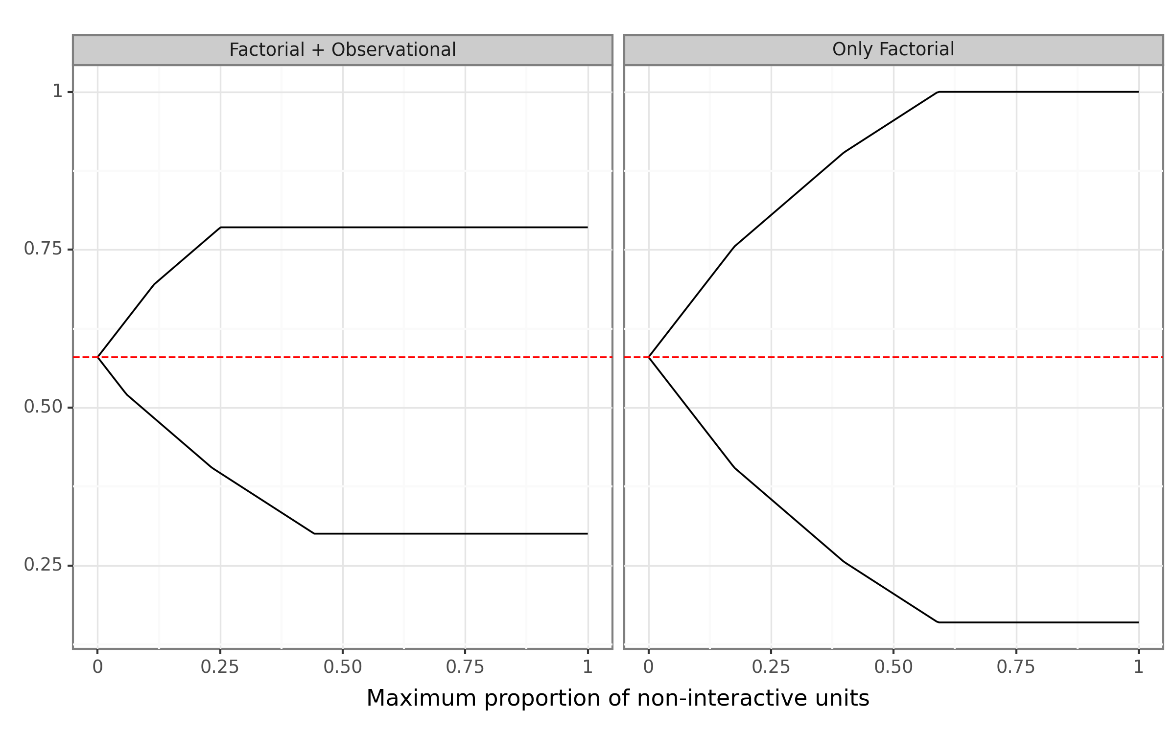
Figure 5: Sensitivity analysis of the ATE, constrained by the proportion of non-interactive units, is presented. The details of the model are introduced in the Supplementary Material (Example 2). The dashed line represents the actual ATE of the model (0.58), while the black lines depict strict bounds corresponding to varying constraints on the maximum proportion of non-interactive units (x-axis). A maximum constraint of 0 implies no interaction, resulting in exact point identification of the ATE. As this maximum constraint increases, the bounds extend to the maximum limits reported in Theorems D.2 and D.1.

4 Simulation

To illustrate the proposed method, I simulate two examples described in the Supplementary Material. The first example involves a structural model with no explicit constraints, while the second one is generated using probabilities over principal strata to enforce both monotonicity and no interaction. Then I generate firstly for each model an example dataset with size equal to $1,000$, both for the observational and for the factorial case (total of $2,000$).

Previously, I discussed identification results tailored to scenarios where researchers have access to population quantities. Here, I delve into the challenge of estimating bounds when dealing with finite samples. In such cases, an additional hurdle arises as it’s not straightforward to estimate confidence intervals for quantities derived from linear programs. Chickering and Pearl, (1996) utilize Bayesian inference via Gibbs’ sampling. Duarte et al., (2023) consider two distinct methods for calculating bounds using autobounds: one based on Kullback-Leibler divergence of Bernoulli distribution, and another utilizing multivariate Gaussian limiting distribution of a Dirichlet. Levis et al., (2023) compute influence functions when incorporating covariates. I remain neutral regarding the proposed solutions. Since the solution provided pertains to identification rather than inference, any of these methods can be employed if the underlying assumptions are justified. To illustrate the bounds with the generated data, I employ bootstrap. So, I generate $1000$ resamples of the generated initial sample and calculate 95% confidence bounds both for the lower bounds and for the upper bounds.

Example 1 was simulated nonparametrically using structural equations, without assuming non-interactivity and monotonicity. The model produced an ATE of 0.24. Two sets of results were estimated: firstly, nonparametric bounds assuming only factorial data, and secondly, nonparametric bounds using both factorial and observational data. These results are depicted in the left panel of Figure 6. The estimated bounds (blue lines) encompass the true ATE value (black lines). The version incorporating both distributions yields bounds superior to the second version. Additionally, I estimated a 95% confidence region (in red) using resampling techniques. In this particular example, one cannot distinguish that the real ATE is different from 0.

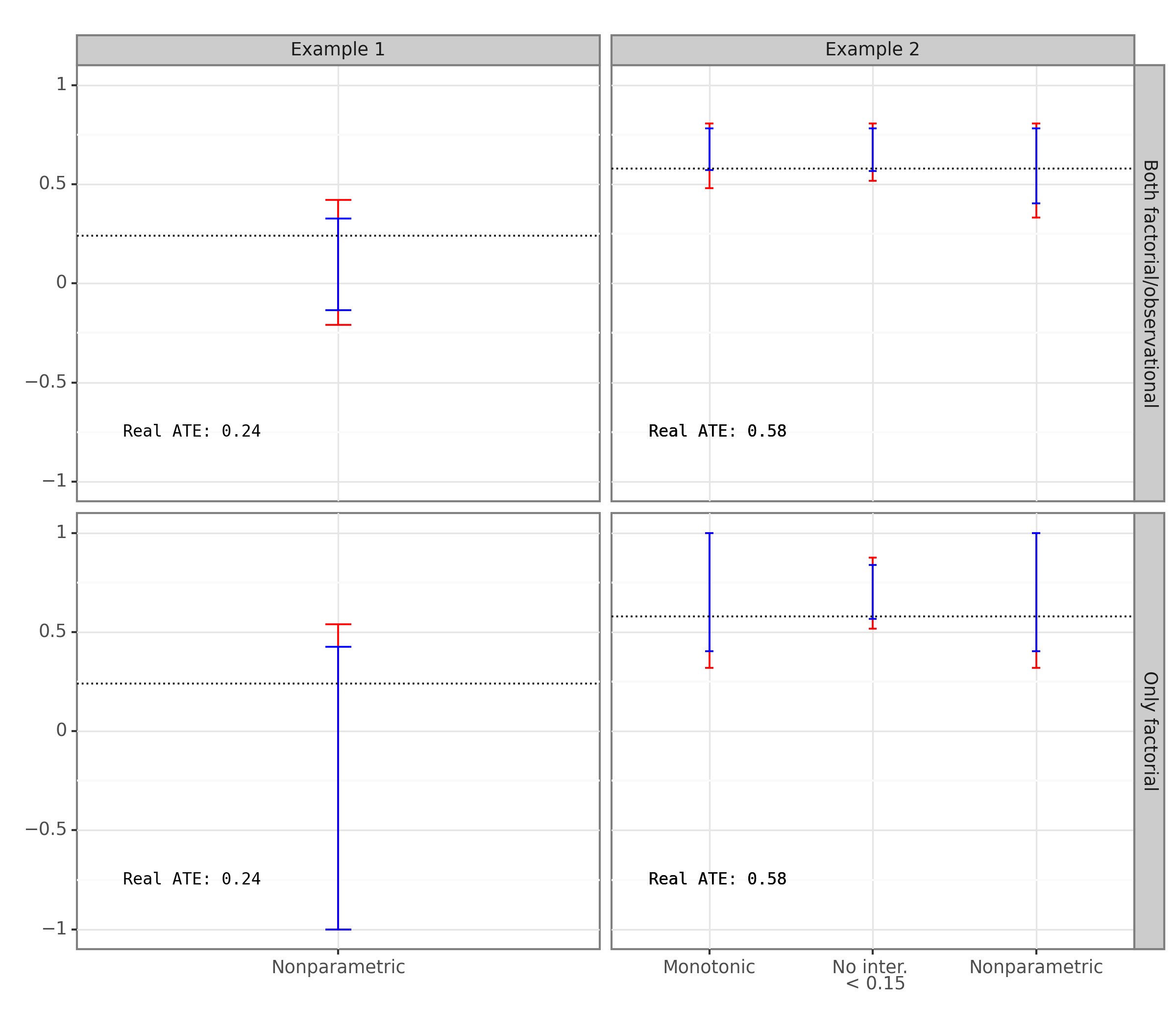
Figure 6: Estimated bounds using simulated data from examples 1 and 2. The blue bars represent the estimated bounds, while the red lines indicate the 95% confidence region for the bounds calculated using bootstrap. The dotted black line shows the true value of the Average Treatment Effect (ATE) for each example: 0.24 for the first and 0.58 for the second. Example 2 explicitly contains only no interactive and monotonic units. Therefore, the analysis for the first model only shows nonparametric bounds. As expected, both bounds cover the real ATE, but those incorporating both factorial and observational data are sharper than those with factorial data alone. For the second example, we estimated three versions: one assuming monotonicity, another assuming a maximum proportion of 0.15 non-interactive units, and a nonparametric version. As expected, the bounds in the nonparametric version are lower than in the other two. In other words, justified restrictive assumptions lead to a quantitative gain in causal information.

In example 2, I explicitly made assumptions of monotonicity and no interaction, with a true ATE of 0.58. This justifies estimating bounds based on these assumptions. As demonstrated, assuming no interaction can lead to point identification results. Rather than adopting this approach, I considered a scenario where one might wish to examine the sensitivity of the no-interaction assumption. In Figure 5, I illustrate bounds conditioned on the maximum proportion of non-interactive units permitted in the model. For instance, if no constraint is imposed and full interactions are allowed, then nonparametric bounds are obtained. All other cases lie between the full interaction and non-interactive point identifiable scenarios. After analyzing the graph, suppose one believes that a maximum of 15% of non-interactive units is reasonable; in that case, the bounds can be evaluated accordingly, along with confidence intervals. This result is depicted in the right panel of Figure 6. Additionally, bounds for the case assuming only monotonicity were included, showing marked improvements compared to the nonparametric scenario. However, all these cases, even when utilizing only the factorial distribution, provide an opportunity to estimate bounds greater than 0 (which can be signed) and encompass the real ATE.

5 Discussion

The paper’s findings highlight that while factorial experiments can significantly reduce the costs associated with estimating multiple treatment effects, they also introduce complexities when estimating single-treatment effects. Specifically, when considering interactions, these effects become non-point-identifiable, and the best approach is to estimate sharp bounds. To address this, I provided bounds for both the nonparametric case and the case assuming monotonicity, aiming to assist researchers in estimating effects under these conditions. Moreover, I outlined a procedure for sensitivity analysis, enabling researchers to justify other assumptions, such as non-interaction, or to test the sensitivity of results to a maximum proportion of non-interactive units. For instance, by limiting interactive units to at most 15%, researchers can still derive meaningful bounds.

Supplementary material

Appendix A Hypothetical Examples

A.1 Example 1

Suppose there are unobserved and observed variables. Assume that the unobserved – represented by variables starting with $U$ – are distributed by binomial distributions with the following parameters:

$$U_{AY}\sim Binom(0.65)$$

$$U_{BY}\sim Binom(0.8)$$

$$U_{Y_{1}}\sim Binom(0.95)$$

$$U_{Y_{2}}\sim Binom(0.9)$$

At last, the functions representing the observed variables $A,B,$ and $Y$ can be defined using logic gates, as they are all binary:

$$A=U_{AY}$$

$$B=U_{BY}$$

$$Y=U_{AY}\land\lnot((U_{Y_{1}}\land B)\oplus(U_{BY}\land U_{Y_{1}}))\oplus(A\oplus U_{Y_{2}})$$

Here, $\land$ denotes the conjunctive logic gate (AND), $\oplus$ denotes the exclusive disjunction (XOR), and $\lnot$ denotes the negation (NOT).

From this example, one can calculate quantities such as the real ATE, which is equal to $0.24$. However, from the factorial experiment, obtained quantities refer not to interventions exclusively on $A$, but on $A$ and $B$ at the same time. In particular, the difference of the expected value of $Y$ given interventions on $A=a_{1}$ and $A=a_{0}$, given that we also had an intervention on $B=b$ are respectively, $-0.55$ and $0.042$, for the cases where $B=b_{0}$ and $B=b_{1}$. Surprisingly, one finds out that using the estimator described by the first researcher – which averages those differences according to a uniform distribution, i.e. $P(B=b_{1})=P(B=b_{0})=0.5$ – then the estimated value will be equal to $-0.25$. Alternatively, using the estimator described by the second researcher – which employs the population distribution of $B$ – the estimated value will be equal to $-0.07$. Therefore, contrarily to the real positive value of the ATE, we obtained two negative estimates. In fact, one can realize that there is no distribution over $B$ that can combine the factorial differences into the real ATE. This implies any attempt to use factorial experiments to answer queries concerning marginal treatments will necessarily be biased. I refer to the bias induced when extrapolating from factorial experiments to in-the-wild effects of isolated treatments as F-bias.

Example 2

Differently from the previous example, I simulate this case according to the specified canonical model and principal strata. The values of each parameter are available in table 3. I assign values for each strata of $A$ and $B$, represented in the columns, and to $Y$, represented in the rows. For notation economy, the strata for $Y$, $\Pr(Y_{a_{0},b_{0}}=i,Y_{a_{0},b_{1}}=j,Y_{a_{1},b_{0}}=k,Y_{a_{1},b_{1}}=l)$, is abbreviated to $y_{ijkl}$. The cells indicate $\Pr(y_{ijkl}|a,b)$ for all values of $A$ and $B$. So, to obtain the joint probability, one has to multiply them by $\Pr(a,b)$, distributed as $\Pr(A=a_{0},B=b_{0})=0.15,\Pr(A=a_{0},B=b_{1})=0.5,\Pr(A=a_{1},B=b_{0})=0.1,\Pr(A=a_{1},B=b_{1})=0.25$.

In particular, all non-monotonic and non-interactive strata were set to have probability equal to $0$. So only probability over the strata $y_{0000},y_{0101},y_{0011},y_{1111}$ were allowed. This model yields an ATE $0.58$. Eventual calculations are provided in the attached python code.

Table 3: Strata for a causal model of $A$ and $B$ causing $Y$ and unobserved confounding. Cells indicate $\Pr(Y_{a_{0},b_{0}}=i,Y_{a_{0},b_{1}}=j,Y_{a_{1},b_{0}}=k,Y_{a_{1},b_{1}}=l|a,b)$ abbreviated to $\Pr(y_{ijkl}|a,b)$, where $y_{ijkl}$ is indicated by the rows and $a,b$ by each column.

	$a_{0},b_{0}$	$a_{0},b_{1}$	$a_{1},b_{0}$	$a_{1},b_{1}$
$y_{0000}$	0.05	0.09	0.05	0.12
$y_{0001}$	0.0	0.0	0.0	0.0
$y_{0010}$	0.0	0.0	0.0	0.0
$y_{0011}$	0.7	0.6	0.5	0.5
$y_{0100}$	0.0	0.0	0.0	0.0
$y_{0101}$	0.1	0.1	0.02	0.03
$y_{0110}$	0.0	0.0	0.0	0.0
$y_{0111}$	0.0	0.0	0.0	0.0
$y_{1000}$	0.0	0.0	0.0	0.0
$y_{1001}$	0.0	0.0	0.0	0.0
$y_{1010}$	0.0	0.0	0.0	0.0
$y_{1011}$	0.0	0.0	0.0	0.0
$y_{1100}$	0.0	0.0	0.0	0.0
$y_{1101}$	0.0	0.0	0.0	0.0
$y_{1110}$	0.0	0.0	0.0	0.0
$y_{1111}$	0.15	0.21	0.43	0.35

Appendix B Non-identifiability results

Theorem B.1.

Consider treatments $A$ and $B$, along with an outcome $Y$. Assume that both $A$ and $B$ independently cause $Y$, without causing each other. Additionally, suppose the effects of both $A$ and $B$ on $Y$ are monotonic, meaning $\Pr(Y_{a_{0}}=y_{1},Y_{a_{1}}=y_{0})=\Pr(Y_{b_{0}}=y_{1},Y_{b_{1}}=y_{0})=0$. Under these conditions, without imposing any other assumptions, such as absence of confounding between $A$, $B$, and $Y$, the probability distribution $\Pr(Y_{a})$, representing the outcome under different levels of treatment $A$, is not identifiable solely from the joint distribution $\Pr(Y_{a,b})$ and $\Pr(Y,A,B)$. Furthermore, the Average Treatment Effect (ATE), defined as the difference in probabilities between different treatment levels, $\Pr(Y_{a}=y)-\Pr(Y_{a^{\prime}}=y)$, remains unidentifiable. Finally, these quantities are not identifiable even if we relax the assumption of monotonicity or if we only have observational or factorial data alone.

Proof.

The proof employs a counterexample using binary variables $A$, $B$, and $Y$. Two models, denoted $M_{0}$ and $M_{1}$, are constructed such that they exhibit monotonicity of $A$ and $B$ on $Y$ and share the same distributions over $\Pr(A,B,Y)$ and $\Pr(Y_{a,b})$. However, they diverge in terms of the distributions of $\Pr(Y_{a})$ and $\Pr(Y_{a})-\Pr(Y_{a^{\prime}})$.

Model specification:

Consider models $M_{0}$ and $M_{1}$, where errors in both models are determined by three independent variables: binary $U_{ay}$, binary $U_{by}$, and ternary $U_{y}$. The probabilities are specified as $\Pr(U_{ay}=1)=\Pr(U_{by}=1)=0.5$, $\Pr(U_{y}=2)=1/5$, and $\Pr(U_{y}=1)=\Pr(U_{y}=0)=2/5$.

In both models, the functions determining $A$ and $B$ are set equal to $A=U_{ay}$ and $B=U_{by}$, meaning both variables are equal to the respective errors.

Now, let the outcome $Y$ for model $0$, $Y_{M_{0}}$, be determined by:

$$Y_{M_{0}}=\begin{cases}\max\{A,B\},&\text{ if }U_{ay}=U_{by}=0\ \text{ and }\ U_{y}=2,\\ B,&\text{ if }U_{ay}=U_{by}=0\ \text{ and }\ U_{y}=1,\\ 1,&\text{ otherwise }\end{cases}$$

Also let $Y$ for model $M_{1}$, $Y_{M_{1}}$ be equal to:

$$Y_{M_{1}}=\begin{cases}\max\{A,B\},&\text{ if }U_{ay}=U_{by}=0\ \text{ and }\ U_{y}\neq 0,\\ \max\{1-A,B\},&\text{ if }U_{ay}=0,U_{by}=1\ \text{ and }\ U_{y}\neq 0,\\ 1,&\text{ otherwise }\end{cases}$$

Observational Data:

For data generated by model $M_{0}$, if $A$ or $B$ equals $1$, then $Y$ must also equal $1$, implying probabilities of $0$ for scenarios where $Y=0$ under those conditions and $0.25$ for scenarios where $Y=1$ under the same conditions. When $A=B=0$, there are three possibilities: if $U_{y}=2$ or $U_{y}=1$, then $Y=0$, and if $U_{y}=0$, then $Y=1$. This yields probabilities of $3/5$ for $Y=0$ and $2/5$ for $Y=1$.

For data generated by model $M_{1}$, if $A=1$, then $Y$ must equal $1$, resulting in probabilities of $0$ for scenarios where $Y=0$ and $0.25$ for scenarios where $Y=1$. If $A=0$ and $B=1$, then $Y$ is always $1$, independently of $U_{y}$, leading to probabilities of $0$ for $Y=0$ and $0.25$ for $Y=1$. When $U_{ay}=U_{by}=0$, there are two possibilities: if $U_{y}=2$ or $U_{y}=1$, then $Y=0$, and if $U_{y}=0$, then $Y=1$, resulting in probabilities of $3/5$ for $Y=0$ and $2/5$ for $Y=1$.

Factorial Data:

In both models $M_{0}$ and $M_{1}$, when $B$ is forced to be $1$, $Y$ is always $1$. If $B$ is forced to be $0$, and $A$ is also forced to be $0$, then $Y$ is $0$ when $U_{ay}=U_{by}=0$ and $U_{y}\neq 0$, resulting in probabilities of $0.15$ for $Y=0$ and $0.85$ for $Y=1$. If $A$ is forced to be $1$, then $Y$ is $0$ when $U_{ay}=U_{by}=0$ and $U_{y}=1$, leading to probabilities of $0.1$ for $Y=0$ and $0.9$ for $Y=1$.

Monotonicity:

Additionally, both models satisfy monotonicity with respect to $A$ and $B$. There are no cases where $Y_{a=1}=0$ and $Y_{a=0}=1$ in model $M_{1}$, and in model $M_{0}$, the only such case occurs when $Y=B$, which remains unchanged if $A$ is set to $0$. Similarly, there are no cases where $Y_{b=1}=0$ and $Y_{b=0}=1$ due to the nature of $Y$ in both models.

These analyses reveal that the observational and factorial quantities are equal in both monotonic models. Now we consider the single-treatment quantities. A summary of all those quantities is included in Table 4.

Single-treatment quantities:

When $A$ is set to $0$ regardless of $B$ in both models $M_{0}$ and $M_{1}$, only one scenario results in $Y=0$: when $U_{ay}=U_{by}=0$ and $U_{y}\neq 0$. This yields $\Pr_{M_{0}}(Y_{A=0}=0)=\Pr_{M_{1}}(Y_{A=0}=0)=0.15$. However, when $A$ is forced to be $1$, in model $M_{0}$, $Y$ consistently equals $1$ across all scenarios. Yet, in model $M_{1}$, there’s a case where $Y=0$ when $U_{ay}=U_{by}=0$ and $U_{y}=1$, with a probability of $0.1$. Thus, $\Pr_{M_{0}}(Y_{A=1}=1)=1$, different from $\Pr_{M_{1}}(Y_{A=1}=1)=0.9$. Consequently, $ATE_{M_{0}}=0.15$, in contrast to $ATE_{M_{1}}=0.05$. This disparity demonstrates that both $\Pr(Y_{A=1})$ and the ATE lack point identifiability.

Table 4: Calculated probabilities for models $M_{0}$ and $M_{1}$ as presented in the counterexample detailed in Theorem B.1. Despite both models being monotonic, they agree on all observational and factorial (2-treatment) quantities. However, they diverge regarding $\Pr(Y_{A=1})$, making not only this probability but also the Average Treatment Effect (ATE) non-identifiable

Probability	Model $M_{0}$	Model $M_{1}$
Observational
$\Pr(A=0,B=0,Y=0)$	0.15	0.15
$\Pr(A=0,B=1,Y=0)$	0	0
$\Pr(A=1,B=0,Y=0)$	0	0
$\Pr(A=1,B=1,Y=0)$	0	0
$\Pr(A=0,B=0,Y=1)$	0.1	0.1
$\Pr(A=0,B=1,Y=1)$	0.25	0.25
$\Pr(A=1,B=0,Y=1)$	0.25	0.25
$\Pr(A=1,B=1,Y=1)$	0.25	0.25
2-Treatment
$\Pr(Y_{A=0,B=0}=1)$	0.85	0.85
$\Pr(Y_{A=0,B=1}=1)$	1	1
$\Pr(Y_{A=1,B=0}=1)$	0.9	0.9
$\Pr(Y_{A=1,B=1}=1)$	1	1
1-Treatment
$\Pr(Y_{A=1}=1)$	1	0.9
$\Pr(Y_{A=0}=1)$	0.85	0.85

The non-identification result demonstrated persists if we relax monotonicity or if we have only factorial, as those scenarios are less restrictive. ∎

Theorem B.2.

Consider treatments $A$ and $B$, along with an outcome $Y$. Assume that both $A$ and $B$ independently cause $Y$, without causing each other. Additionally, suppose the effects of both $A$ and $B$ on $Y$ are monotonic, meaning $\Pr(Y_{a_{0}}=y_{1},Y_{a_{1}}=y_{0})=\Pr(Y_{b_{0}}=y_{1},Y_{b_{1}}=y_{0})=0$, and that there are no interactions, meaning $\Pr(Y_{a,b}=y_{1})-\Pr(Y_{a^{\prime},b}=y_{1})=\Pr(Y_{a,b^{\prime}}=y_{1})-\Pr(Y_{a^{\prime},b^{\prime}}=y_{1})$ and $\Pr(Y_{a,b}=y_{1})-\Pr(Y_{a,b^{\prime}}=y_{1})=\Pr(Y_{a^{\prime},b}=y_{1})-\Pr(Y_{a^{\prime},b^{\prime}}=y_{1})$. Under these conditions, without imposing any other assumptions, such as absence of confounding between $A$, $B$, and $Y$, the probability distribution $\Pr(Y_{a})$, representing the outcome under different levels of treatment $A$, is not identifiable solely from the joint distribution $\Pr(Y_{a,b})$ and $\Pr(Y,A,B)$. Finally, these quantities are not identifiable even if we relax the assumption of monotonicity.

Proof.

Under monotonicity and no interaction assumptions, there are only four possible functions from $A,B$ to $Y$: $Y=1,Y=A,Y=B,Y=0$. We construct two different models, $M_{0}$ and $M_{1}$ using those functions that induce the same observational and factorial distribution, but that diverge with respect to single-treatment quantities.

Consider models $M_{0}$ and $M_{1}$, where errors in both models are determined by two independent variables: a ternary $U_{aby}$ with probabilities $\Pr(U_{aby}=0)=0.1,\Pr(U_{aby}=1)=0.3,\Pr(U_{aby}=2)=0.6$ and a ternary uniform $U_{y}$ with $\Pr(U_{y}=u)=1/3$ for any $u$. Let $A=0$, if $\Pr(U_{aby}=0)$ and $A=1$, if $\Pr(U_{aby}\neq 0)$. Let $B=0$, if $\Pr(U_{aby}\neq 2)$ and $B=1$, if $\Pr(U_{aby}=2)$.

Let $Y_{M_{0}}$ be determined by the function:

$$Y_{M_{0}}=\begin{cases}0,\text{ if }&U_{aby}=1,U_{y}=0\\ 1,\text{ if }&U_{aby}=1,U_{y}=1\\ B,\text{ if }&U_{aby}=0,U_{y}=0\text{ or }U_{aby}=2,U_{y}\neq 0\\ A,\text{ otherwise }&\end{cases}$$

Let $Y_{M_{1}}$ be determined by the function:

$$Y_{M_{1}}=\begin{cases}0,\text{ if }&U_{aby}=1,U_{y}=0\\ 1,\text{ if }&U_{aby}=1,U_{y}=1\\ B,\text{ if }&U_{aby}=2,\\ A,\text{ otherwise }&\end{cases}$$

Computation was omitted, but outputs are presented in Table 5, which show that both $\Pr_{M_{0}}(A,B,Y)=\Pr_{M_{1}}(A,B,Y)$ and $\Pr_{M_{0}}(Y_{a,b})=\Pr_{M_{1}}(Y_{a,b})$ but $\Pr_{M_{0}}({Y_{a}})\neq\Pr_{M_{1}}({Y_{a}})$. That suffices to show $\Pr({Y_{a}})$ is not identifiable. ∎

Table 5: Calculated probabilities for models $M_{0}$ and $M_{1}$ as presented in the counterexample detailed in Theorem B.2. Despite both models being monotonic, they agree on all observational and factorial (2-treatment) quantities. However, they diverge regarding $\Pr(Y_{A=1})$ and $\Pr(Y_{A=0})$. That implies both quantities are not point-identifiable.

Probability	Model $M_{0}$	Model $M_{1}$
Observational
$\Pr(A=0,B=0,Y=0)$	0.1	0.1
$\Pr(A=0,B=1,Y=0)$	0	0
$\Pr(A=1,B=0,Y=0)$	0	0
$\Pr(A=1,B=1,Y=0)$	0	0
$\Pr(A=0,B=0,Y=1)$	0.1	0.1
$\Pr(A=0,B=1,Y=1)$	0.2	0.2
$\Pr(A=1,B=0,Y=1)$	0	0
$\Pr(A=1,B=1,Y=1)$	0.6	0.6
2-Treatment
$\Pr(Y_{A=0,B=0}=1)$	0.1	0.1
$\Pr(Y_{A=0,B=1}=1)$	0.4	0.4
$\Pr(Y_{A=1,B=0}=1)$	0.6	0.6
$\Pr(Y_{A=1,B=1}=1)$	0.9	0.9
1-Treatment
$\Pr(Y_{A=1}=1)$	0.8	0.9
$\Pr(Y_{A=0}=1)$	0.3	0.4

In the scenario outlined in Theorem B.2, if we remove the assumption of monotonicity, $\Pr(Y_{a})$ remains unidentifiable solely from the joint distribution $\Pr(Y_{a,b})$ and $\Pr(Y,A,B)$. This is due to the fact that the non-identification result remains in less restrictive cases.

Theorem B.3.

Consider treatments $A$ and $B$, along with an outcome $Y$. Assume that both $A$ and $B$ independently cause $Y$, without causing each other. Additionally, suppose the effects of both $A$ and $B$ on $Y$ are monotonic, meaning $\Pr(Y_{a_{0}}=y_{1},Y_{a_{1}}=y_{0})=\Pr(Y_{b_{0}}=y_{1},Y_{b_{1}}=y_{0})=0$, and that there are no interactions, meaning $\Pr(Y_{a,b}=y_{1})-\Pr(Y_{a^{\prime},b}=y_{1})=\Pr(Y_{a,b^{\prime}}=y_{1})-\Pr(Y_{a^{\prime},b^{\prime}}=y_{1})$ and $\Pr(Y_{a,b}=y_{1})-\Pr(Y_{a,b^{\prime}}=y_{1})=\Pr(Y_{a^{\prime},b}=y_{1})-\Pr(Y_{a^{\prime},b^{\prime}}=y_{1})$. Under these conditions, without imposing any other assumptions, such as absence of confounding between $A$, $B$, and $Y$, the probability distribution $\Pr(Y_{a})$, representing the outcome under different levels of treatment $A$, is not identifiable solely from the factorial distribution $\Pr(Y_{a,b})$ or from observational distribution $\Pr(y,a,b)$ alone. Furthermore, only in the last case, (observational distribution alone), the ATE remains unidentifiable.

Proof.

Consider two models $M_{0}$ and $M_{1}$ on binary $A,B$ and $Y$. Assume we fix the probability under interventions (factorial data) on $B$ and $A$, $\Pr_{M=0}(Y_{a,b})=\Pr_{M=1}(Y_{a,b})$ and that monotonicity is satisfied. As $B$ is independent of $Y_{a,b}$, set $\Pr_{M=0}(b)\neq\Pr_{M=0}(b)$.

Now assume we rather have only observational data, $\Pr(y,a,b)$. In this case, as we have unobserved confounding, $Y_{a}$ or the ATE would not be identifiable. Those results remain, even if we assume monotonicity, provided that non-identification results persist in less restrictive scenarios.

∎

Appendix C Parametric Identification of Single-Treatment Estimands Using Factorial Data

Theorem C.1 (Additive separability is sufficient for identifiability of the ATE).

Suppose $y_{i}=f(a_{i},u_{i})+g(b_{i},u_{i})$ with unobserved $u_{i}$ for arbitrary fixed functions $f,g$ is a model of the real-world and assume statistical dependence between $a_{i}$ and $b_{i}$ and $u_{i}$.

Suppose one has data on $\Pr(Y(a,b))$, for all states $a,b,y$. Then the ATE of $A$ on $Y$ is identifiable by

$$\sum_{b}(\operatorname{\mathbb{E}}(Y_{a,b})-\operatorname{\mathbb{E}}(Y_{a^{\prime},b}))f(b),\text{ with uniform }f(b)$$ (4)

Proof.

Suppose $y_{i}=f(a_{i},u_{i})+g(b_{i},u_{i})$ for arbitrary functions $f,g$, then $E(Y_{a})=\operatorname{\mathbb{E}}(f(a,u_{i}))+\operatorname{\mathbb{E}}(g(b_{i},u_{i}))$ and $\operatorname{\mathbb{E}}(Y_{a^{\prime}})=\operatorname{\mathbb{E}}(f(a^{\prime},u_{i}))+\operatorname{\mathbb{E}}(g(b_{i}))$. Then the ATE is $\operatorname{\mathbb{E}}(Y_{a}-Y_{a^{\prime}})=\operatorname{\mathbb{E}}(f(a,u_{i})-f(a^{\prime},u_{i}))$.

So it is sufficient to identify $\operatorname{\mathbb{E}}(f(a,u_{i})-f(a^{\prime},u_{i}))$. Using the factorial data we have the following identifiable equality for any $b\in\operatorname{supp}(B)$:

$$\operatorname{\mathbb{E}}(Y_{a,b})=\operatorname{\mathbb{E}}(f(a,u_{i}))+\operatorname{\mathbb{E}}(g(b,u_{i})),$$

Then $\operatorname{\mathbb{E}}(Y_{a}-Y_{a^{\prime}})=\operatorname{\mathbb{E}}(f(a,u_{i})-f(a^{\prime},u_{i}))$ is identifiable by either $\operatorname{\mathbb{E}}(Y_{a,b})-\operatorname{\mathbb{E}}(Y_{a^{\prime},b})$ for any $b$. That implies that the for a uniform distribution $f(b)$, the ATE is also identified by $\sum_{b\in\operatorname{supp}(B)}(\operatorname{\mathbb{E}}(Y_{a_{1},b})-\operatorname{\mathbb{E}}(Y_{a_{0},b}))f(b)$.

∎

The separability criterion described above does not accept interactions. However, for linear models with interactions, identifiability is still possible.

Theorem C.2 (Sufficiency of Interactive Linearity For Single-treatment Quantities).

Suppose $y_{i}=\beta_{0}+\beta_{1}a_{i}+\beta_{2}b_{i}+\beta_{3}a_{i}b_{i}+u_{i}$ with unobserved $u_{i}$ is a model of the real-world, discrete $b_{i}$ and $a_{i}$, and assume statistical dependence between $a_{i}$ and $b_{i}$ and $u_{i}$. Then the the expected outcome of an intervention $A=a$ is identifiable using the observational quantity $\Pr(B=b)$ and the factorial distribution $\operatorname{\mathbb{E}}(Y_{a,b})$ by:

$$\operatorname{\mathbb{E}}(Y_{a})=\sum_{b}\operatorname{\mathbb{E}}(Y_{a,b})\Pr(b)$$ (5)

and the ATE is by the quantity:

$$\operatorname{\mathbb{E}}(Y_{a})-\operatorname{\mathbb{E}}(Y_{a^{\prime}})=\sum_{b}(\operatorname{\mathbb{E}}(Y_{a,b})-\operatorname{\mathbb{E}}(Y_{a^{\prime},b}))\Pr(b)$$

Proof.

We make the simplifying assumption that $\operatorname{\mathbb{E}}(u_{i})=0$. Then we can rewrite $\operatorname{\mathbb{E}}(Y_{a})$ as:

$$\operatorname{\mathbb{E}}(Y_{a})=$$

$$\beta_{0}+\beta_{1}\cdot a+\beta_{2}\operatorname{\mathbb{E}}(b_{i})+\beta_{3}\operatorname{\mathbb{E}}(b_{i})\cdot a$$

As $\Pr(b)$ is directly identifiable from the observational data and $\operatorname{\mathbb{E}}(Y_{a,b})$ from the factorial data, then:

$$\sum_{b}\operatorname{\mathbb{E}}(Y_{a,b})\Pr(b)=$$

$$\sum_{b}\Pr(b)(\beta_{0}+\beta_{1}a+\beta_{2}b+\beta_{3}ab)=$$

$$\beta_{0}\sum_{b}\Pr(b)+\beta_{1}a\sum_{b}\Pr(b)+\beta_{2}\sum_{b}b\Pr(b)+\beta_{3}a\sum_{b}b\Pr(b)=$$

$$\beta_{0}+\beta_{1}a+\beta_{2}\operatorname{\mathbb{E}}(b_{i})+a\beta_{3}\operatorname{\mathbb{E}}(b_{i})=$$

$$\operatorname{\mathbb{E}}(Y_{a})$$

That confirms that the identification of $\operatorname{\mathbb{E}}(Y_{a})=\sum_{b}\operatorname{\mathbb{E}}(Y_{a,b})\Pr(b)$ and implies that the ATE is identifiable by

$$\operatorname{\mathbb{E}}(Y_{a}-Y_{a^{\prime}})=\sum_{b}(\operatorname{\mathbb{E}}(Y_{a,b})-\operatorname{\mathbb{E}}(Y_{a^{\prime},b}))\Pr(b)$$

∎

Corollary C.2.1 (Linearity is Sufficient for Identifiability).

Suppose $y_{i}=\beta_{0}+\beta_{1}a_{i}+\beta_{2}b_{i}+u_{i}$ with unobserved $u_{i}$ is a model of the real-world and assume statistical dependence between $a_{i}$ and $b_{i}$ and $u_{i}$. Then the ATE of $A$ on $Y$ is identifiable using factorial data by the quantity in equation 4 as that is a case of additive separability (Theorem C.1). Additionally, linearity is also a case of interactive linearity (Theorem C.2), so single-treatment quantities are identifiable by Equation 5. Finally, observational data alone is insufficient for identifiability given the standard omitted variable bias (unobserved confounding).

Appendix D Partial identification results

Theorem D.1 (Bounds only with factorial distribution).

Suppose $A,B,Y$ are binary random variables and we have only factorial data – $\Pr(Y_{a,b})$. Then the sharp bounds for the expected value of $Y$ given intervention on $A$, $\Pr(Y_{a})$ are:

$$\max\{0,1-\sum_{b}\Pr(Y_{ab}\neq y)\}\leq\Pr(Y_{a})\leq\min\{\sum_{b}\Pr(Y_{ab}=y),1\}$$

and the bounds for the ATE ( $\operatorname{\mathbb{E}}(Y_{a_{1}}-Y_{a_{0}}$) are:

$$\max\begin{cases}-1\\ -\operatorname{\mathbb{E}}(Y_{a_{0}b_{0}}+Y_{a_{0}b_{1}})\\ \operatorname{\mathbb{E}}(Y_{a_{1}b_{0}}+Y_{a_{1}b_{1}})-2\\ \operatorname{\mathbb{E}}(Y_{a_{1}b_{0}}+Y_{a_{1}b_{1}}-Y_{a_{0}b_{0}}-Y_{a_{0}b_{1}})-1\end{cases}\leq\text{ATE}\leq\min\begin{cases}1\\ 2-\operatorname{\mathbb{E}}(Y_{a_{0}b_{1}}+Y_{a_{0}b_{0}})\\ \operatorname{\mathbb{E}}(Y_{a_{1}b_{0}}+Y_{a_{1}b_{1}})\\ 1+\operatorname{\mathbb{E}}(Y_{a_{1}b_{0}}+Y_{a_{1}b_{1}}-Y_{a_{0}b_{0}}-Y_{a_{0}b_{1}})\end{cases}$$

Proof.

This result is due to the solution of the linear program detailed in the linear program detailed below. Because that’s the solution for the program, those are also the sharp bounds for the problem (cannot be improved upon). ∎

Theorem D.2 (Bounds with both observational and factorial distributions).

Suppose $A,B,Y$ are binary random variables and we have both factorial – $\Pr(Y_{a,b})$ and observational data – $\Pr(A,B,Y)$. Let $x^{\prime}=1-x$ for any $x$. Then the sharp bounds for a quantity such as the expected value of $Y$ given intervention on $A$, $E(Y_{a})$ are:

$$\max\begin{cases}0,\\ \Pr(Y_{ab^{\prime}}=y)-\Pr(a^{\prime},b)-\Pr(a,b,y^{\prime}),\\ \Pr(a,y),\\ \Pr(Y_{ab}=y^{\prime})-\Pr(b^{\prime},y^{\prime})-\Pr(a^{\prime},b^{\prime},y),\\ \Pr(Y_{ab^{\prime}}=y)-\Pr(Y_{ab}=y^{\prime})\end{cases}\leq\operatorname{\mathbb{E}}(Y_{a})\leq\min\begin{cases}1,\\ \Pr(a^{\prime},b,y^{\prime})+\Pr(b,y)+\Pr(Y_{ab^{\prime}}=y),\\ 1-\Pr(a,y^{\prime}),\\ \Pr(Y_{ab^{\prime}}=y)+\Pr(Y_{ab}=y),\\ \Pr(a^{\prime},b^{\prime})+\Pr(a,b^{\prime},y)+\Pr(Y_{ab}=y)\end{cases}$$

and the sharp lower and upper bounds for the ATE are respectively:

$$\max\begin{cases}-\Pr(a_{1},y_{0})-\Pr(a_{0},y_{1})\\ \Pr(a_{1},y_{1})-\Pr(Y_{a_{0}b_{0}}=y_{1})-\Pr(Y_{a_{0}b_{1}}=y_{1})\\ \Pr(a_{1},b_{1})-\Pr(a_{1},y_{0})-\Pr(a_{0},b_{0},y_{1})-\Pr(Y_{a_{0}b_{1}}=y_{1})\\ \Pr(a_{1},b_{0})-\Pr(a_{1},y_{0})-\Pr(a_{0},b_{1},y_{1})-\Pr(Y_{a_{0}b_{0}}=y_{1})\\ \Pr(a_{0},y_{0})-\Pr(Y_{a_{1}b_{0}}=y_{0})-\Pr(Y_{a_{1}b_{1}}=y_{0})\\ \Pr(Y_{a_{1}b_{0}}=y_{1})-\Pr(Y_{a_{1}b_{1}}=y_{0})-\Pr(Y_{a_{0}b_{0}}=y_{1})-\Pr(Y_{a_{0}b_{1}}=y_{1})\\ \Pr(Y_{a_{1}b_{0}}=y_{1})-\Pr(Y_{a_{1}b_{1}}=y_{0})-\Pr(Y_{a_{0}b_{1}}=y_{1})-\Pr(a_{0},b_{0},y_{1})-\Pr(a_{1},b_{0})\\ \Pr(Y_{a_{1}b_{0}}=y_{1})-\Pr(Y_{a_{1}b_{1}}=y_{0})-\Pr(Y_{a_{0}b_{0}}=y_{1})-\Pr(a_{0},b_{1},y_{1})-\Pr(a_{1},b_{1})\\ \Pr(a_{0},b_{1})-\Pr(a_{1},b_{0},y_{0})-\Pr(a_{0},y_{1})-\Pr(Y_{a_{1}b_{1}}=y_{0})\\ \Pr(Y_{a_{1}b_{1}}=y_{1})-\Pr(Y_{a_{0}b_{0}}=y_{1})-\Pr(Y_{a_{0}b_{1}}=y_{1})-\Pr(a_{1},b_{0},y_{0})-\Pr(a_{0},b_{0})\\ \Pr(Y_{a_{1}b_{1}}=y_{1})-\Pr(Y_{a_{0}b_{1}}=y_{1})-\Pr(b_{0})-\Pr(a_{1},b_{0},y_{0})-\Pr(a_{0},b_{0},y_{1})\\ \Pr(a_{1},b_{0},y_{1})+\Pr(a_{0},b_{1},y_{0})-\Pr(Y_{a_{1}b_{1}}=y_{0})-\Pr(Y_{a_{0}b_{0}}=y_{1})\\ \Pr(a_{0},b_{0})-\Pr(a_{1},b_{1},y_{0})-\Pr(a_{0},y_{1})-\Pr(Y_{a_{1}b_{0}}=y_{0})\\ \Pr(Y_{a_{1}b_{0}}=y_{1})-\Pr(Y_{a_{0}b_{0}}=y_{1})-\Pr(Y_{a_{0}b_{1}}=y_{1})-\Pr(a_{0},b_{1})-\Pr(a_{1},b_{1},y_{0})\\ \Pr(a_{1},b_{1},y_{1})+\Pr(a_{0},b_{0},y_{0})-\Pr(Y_{a_{1}b_{0}}=y_{0})-\Pr(Y_{a_{0}b_{1}}=y_{1})\\ \Pr(Y_{a_{1}b_{0}}=y_{1})-\Pr(Y_{a_{0}b_{1}}=y_{1})-\Pr(a_{0},b_{1})-\Pr(a_{1},b_{1},y_{0})-\Pr(a_{0},b_{1},y_{1})-\Pr(a_{1},b_{1})\end{cases}$$

and

$$\min\begin{cases}\Pr(a_{1},y_{1})+\Pr(a_{0},y_{0})\\ \Pr(Y_{a_{0}b_{0}}=y_{0})+\Pr(Y_{a_{0}b_{1}}=y_{0})-\Pr(a_{1},y_{0})\\ \Pr(Y_{a_{0}b_{1}}=y_{0})+\Pr(a_{0},b_{0},y_{0})+\Pr(a_{1},b_{0})-\Pr(a_{1},y_{0})\\ \Pr(Y_{a_{0}b_{0}}=y_{0})+\Pr(a_{0},b_{1},y_{0})+\Pr(a_{1},b_{1})-\Pr(a_{1},y_{0})\\ \Pr(Y_{a_{1}b_{0}}=y_{1})+\Pr(Y_{a_{1}b_{1}}=y_{1})-\Pr(a_{0},y_{1})\\ \Pr(Y_{a_{1}b_{0}}=y_{1})+\Pr(Y_{a_{1}b_{1}}=y_{1})+\Pr(Y_{a_{0}b_{0}}=y_{0})-\Pr(Y_{a_{0}b_{1}}=y_{1})\\ \Pr(Y_{a_{1}b_{0}}=y_{1})+\Pr(Y_{a_{1}b_{1}}=y_{1})-\Pr(Y_{a_{0}b_{1}}=y_{1})+\Pr(b_{0},y_{0})+\Pr(a_{1},b_{0},y_{1})\\ \Pr(Y_{a_{1}b_{0}}=y_{1})+\Pr(Y_{a_{1}b_{1}}=y_{1})-\Pr(Y_{a_{0}b_{0}}=y_{1})+\Pr(b_{1},y_{0})+\Pr(a_{1},b_{1},y_{1})\\ \Pr(Y_{a_{1}b_{1}}=y_{1})+\Pr(a_{1},b_{0},y_{1})+\Pr(a_{0},b_{0},y_{0})-\Pr(a_{0},b_{1},y_{1})\\ \Pr(Y_{a_{1}b_{1}}=y_{1})+\Pr(Y_{a_{0}b_{1}}=y_{0})-\Pr(Y_{a_{0}b_{0}}=y_{1})+\Pr(a_{0},b_{0})+\Pr(a_{1},b_{0},y_{1})\\ \Pr(Y_{a_{1}b_{1}}=y_{1})-\Pr(Y_{a_{0}b_{1}}=y_{1})+\Pr(a_{0},b_{0})+\Pr(b_{0},y_{0})+2\Pr(a_{1},b_{0},y_{1})\\ \Pr(Y_{a_{1}b_{1}}=y_{1})+\Pr(Y_{a_{0}b_{0}}=y_{0})-\Pr(a_{1},b_{0},y_{0})-\Pr(a_{0},b_{1},y_{1})\\ \Pr(Y_{a_{1}b_{0}}=y_{1})-\Pr(a_{0},b_{0})+\Pr(a_{1},b_{1},y_{1})+\Pr(a_{0},y_{0})\\ \Pr(Y_{a_{1}b_{0}}=y_{1})-\Pr(Y_{a_{0}b_{0}}=y_{1})+\Pr(Y_{a_{0}b_{1}}=y_{0})+\Pr(a_{0},b_{1})+\Pr(a_{1},b_{1},y_{1})\\ \Pr(Y_{a_{1}b_{0}}=y_{1})-\Pr(Y_{a_{0}b_{1}}=y_{1})+\Pr(a_{0},b_{1})+\Pr(a_{1},y_{1})+\Pr(b_{0},y_{0})\\ \Pr(Y_{a_{1}b_{0}}=y_{1})-\Pr(Y_{a_{0}b_{0}}=y_{1})+\Pr(a_{0},b_{1})+\Pr(b_{1},y_{0})+2\Pr(a_{1},b_{1},y_{1})\end{cases}$$

Proof.

This result is due to the solution of the linear program detailed in the linear program detailed below. Because that’s the solution for the program, those are also the sharp bounds for the problem (cannot be improved upon). ∎

Theorem D.3 (Bounds with monotonicity and using only factorial distribution).

Suppose $A,B,Y$ are binary random variables and we have only factorial data – $\Pr(Y_{a,b})$. Assume the causal effects of $A$ and $B$ on $Y$ are monotonic. Then the sharp bounds both for the expected value of $Y$ given intervention on $A$, $\Pr(Y_{a}=y_{1})$:

$$0\leq\Pr(Y_{a_{1}}=y_{1})\leq\min\{\sum_{b}\Pr(y_{ab}),1\}$$

, and for the ATE are:

$$\max\begin{cases}0,\\ -\Pr(Y_{a0b0}=y_{0})-\Pr(Y_{a0b1}=y_{1})+\Pr(Y_{a1b0}=y_{0})-\Pr(Y_{a1b1}=y_{0})\\ -\Pr(Y_{a0b0}=y_{1})-\Pr(Y_{a0b1}=y_{0})-\Pr(Y_{a1b0}=y_{0})+\Pr(Y_{a1b1}=y_{0})\\ -\Pr(Y_{a0b0}=y_{`})-\Pr(Y_{a0b1}=y_{1})+\Pr(Y_{a1b0}=y_{1})-\Pr(Y_{a1b1}=y_{0})\\ \end{cases}\leq\text{ ATE }$$

and

$$\text{ ATE }\leq\min\begin{cases}1\\ \Pr(Y_{a0b0}=y_{0})-\Pr(Y_{a0b1}=y_{1})+\Pr(Y_{a1b0}=y_{1})+\Pr(Y_{a1b1}=y_{1})\\ \Pr(Y_{a0b0}=y_{0})+\Pr(Y_{a1b1}=y_{1})\\ \Pr(Y_{a0b1}=y_{0})+\Pr(Y_{a1b0}=y_{1})\\ \Pr(Y_{a1b0}=y_{1})+\Pr(Y_{a1b1}=y_{1})\\ \Pr(Y_{a0b0}=y_{0})+\Pr(Y_{a0b1}=y_{)}\\ \end{cases}$$

Proof.

This result is due to the solution of the linear program detailed in the linear program detailed below. Because that’s the solution for the program, those are also the sharp bounds for the problem (cannot be improved upon). ∎

Theorem D.4 (Bounds with monotonicity and using both distributions).

Suppose $A,B,Y$ are binary random variables and we have both factorial – $\Pr(Y_{a,b})$ and observational data – $\Pr(A,B,Y)$. Assume the causal effects of $A$ and $B$ on $Y$ are monotonic. Then the sharp bounds for a quantity such as the expected value of $Y$ given intervention on $A$, $E(Y_{a_{1}})$ are:

$$\max\begin{cases}0\\ -\Pr(Y_{a_{0}b_{0}}=y_{1})-\Pr(Y_{a_{0}b_{1}}=y_{1})+\Pr(Y_{a_{1}b_{0}}=y_{1})-\Pr(Y_{a_{1}b_{1}}=y_{0})\\ -\Pr(Y_{a_{0}b_{0}}=y_{0})-\Pr(Y_{a_{0}b_{1}}=y_{1})+\Pr(Y_{a_{1}b_{0}}=y_{0})-\Pr(Y_{a_{1}b_{1}}=y_{0})\\ \Pr(Y_{a_{0}b_{0}}=y_{0})-\Pr(Y_{a_{0}b_{1}}=y_{0})-\Pr(Y_{a_{1}b_{0}}=y_{0})-\Pr(Y_{a_{1}b_{1}}=y_{1})\\ \end{cases}\leq\operatorname{\mathbb{E}}(Y_{a_{1}})$$

and

$$\operatorname{\mathbb{E}}(Y_{a_{1}})\leq\min\begin{cases}1\\ \Pr(Y_{a_{0}b_{0}}=y_{0})+\Pr(Y_{a_{1}b_{1}}=y_{1})\\ -\Pr(Y_{a_{0}b_{0}}=y_{1})+\Pr(Y_{a_{0}b_{1}}=y_{0})+\Pr(Y_{a_{1}b_{0}}=y_{1})+\Pr(Y_{a_{1}b_{1}}=y_{1})\\ \Pr(Y_{a_{1}b_{0}}=y_{1})+\Pr(Y_{a_{1}b_{1}}=y_{1})\\ \Pr(Y_{a_{0}b_{1}}=y_{0})+\Pr(Y_{a_{1}b_{0}}=y_{1})\\ \Pr(Y_{a_{0}b_{0}}=y_{0})-\Pr(Y_{a_{0}b_{1}}=y_{1})+\Pr(Y_{a_{1}b_{0}}=y_{0})+\Pr(Y_{a_{1}b_{0}}=y_{1})\\ \end{cases}$$

and the sharp lower and upper bounds for the ATE are respectively:

$$\max\begin{cases}0\\ \Pr(b_{0},y_{1})-\Pr(Y_{a_{0}b_{0}}=y_{1})\\ -\Pr(y_{1})-\Pr(a_{0},b_{1},y_{0})+\Pr(Y_{a_{1}b_{0}}=y_{1})\\ -\Pr(a_{0},b_{1})-\Pr(a_{1},b_{1},y_{1})-\Pr(Y_{a_{0}b_{0}}=y_{1})+\Pr(Y_{a_{1}b_{0}}=y_{1})\\ \Pr(a_{0},b_{0},y_{1})+\Pr(b_{1},y_{1})-\Pr(Y_{a_{0}b_{1}}=y_{1})\\ \Pr(y_{1})+\Pr(a_{0},b_{0},y_{1})-\Pr(Y_{a_{0}b_{0}}=y_{1})-\Pr(Y_{a_{0}b_{1}}=y_{1})\\ \Pr(a_{0},b_{0},y_{1})-\Pr(a_{0},b_{1},y_{0})-\Pr(Y_{a_{0}b_{0}}=y_{1})-\Pr(Y_{a_{0}b_{1}}=y_{1})+\Pr(Y_{a_{1}b_{0}}=y_{1})\\ -\Pr(a_{0},b_{1},y_{0})-\Pr(a_{1},b_{0},y_{1})-\Pr(Y_{a_{0}b_{1}}=y_{1})+\Pr(Y_{a_{1}b_{0}}=y_{1})\\ -\Pr(b_{0})-\Pr(b_{1},y_{1})+\Pr(Y_{a_{1}b_{1}}=y_{1})\\ -\Pr(b_{1},y_{1})-\Pr(b_{0},y_{0})-\Pr(Y_{a_{0}b_{0}}=y_{1})+\Pr(Y_{a_{1}b_{1}}=y_{1})\\ -\Pr(y_{1})+\Pr(a_{1},b_{1},y_{0})-\Pr(Y_{a_{1}b_{0}}=y_{0})+\Pr(Y_{a_{1}b_{1}}=y_{1})\\ -\Pr(b_{1},y_{1})+\Pr(a_{1},b_{1},y_{0})-\Pr(Y_{a_{0}b_{0}}=y_{1})-\Pr(Y_{a_{1}b_{0}}=y_{0})+\Pr(Y_{a_{1}b_{1}}=y_{1})\\ -\Pr(b_{0},y_{0})-\Pr(a_{1},b_{0},y_{1})-\Pr(Y_{a_{0}b_{1}}=y_{1})+\Pr(Y_{a_{1}b_{1}}=y_{1})\\ -\Pr(a_{0},b_{0})-\Pr(a_{1},b_{0},y_{0})-\Pr(Y_{a_{0}b_{0}}=y_{1})-\Pr(Y_{a_{0}b_{1}}=y_{1})+\Pr(Y_{a_{1}b_{1}}=y_{1})\\ \Pr(a_{1},b_{0},y_{1})+\Pr(a_{1},b_{0},y_{1})-\Pr(Y_{a_{0}b_{0}}=y_{1})-\Pr(Y_{a_{0}b_{1}}=y_{1})-\Pr(Y_{a_{1}b_{0}}=y_{0})+\Pr(Y_{a_{1}b_{1}}=y_{1})\\ -\Pr(a_{0})-\Pr(a_{1},b_{0})-\Pr(a_{1},y_{1})-\Pr(Y_{a_{0}b_{1}}=y_{1})+\Pr(Y_{a_{1}b_{0}}=y_{1})+\Pr(Y_{a_{1}b_{1}}=y_{1})\end{cases}$$

and

$$\min\begin{cases}-\Pr(a_{0},b_{0},y_{1})+\Pr(a_{0},b_{1},y_{0})+\Pr(a_{1},b_{1},y_{1})+\Pr(Y_{a_{1}b_{0}}=y_{1})\\ \Pr(a_{0},b_{0},y_{0})+\Pr(a_{1},b_{0},y_{1})+\Pr(a_{1},b_{1},y_{0})+\Pr(Y_{a_{0}b_{1}}=y_{0})\\ \Pr(a_{0},b_{0},y_{0})+\Pr(b_{0})-\Pr(Y_{a_{0}b_{1}}=y_{1})+\Pr(Y_{a_{1}b_{1}}=y_{1})\\ \Pr(a_{0},y_{0})+\Pr(a_{1},y_{1})\\ \Pr(a_{0},y_{0})+\Pr(b_{1},y_{1})+\Pr(a_{1},b_{0})-\Pr(Y_{a_{0}b_{1}}=y_{1})+\Pr(Y_{a_{1}b_{0}}=y_{1})\\ \Pr(b_{1})+\Pr(a_{1},b_{1},y_{1})-\Pr(Y_{a_{0}b_{0}}=y_{1})+\Pr(Y_{a_{1}b_{0}}=y_{1})\\ -\Pr(a_{0},b_{1},y_{0})-\Pr(a_{1},y_{0})+\Pr(Y_{a_{0}b_{0}}=y_{0})+\Pr(Y_{a_{0}b_{1}}=y_{0})\\ \Pr(b_{0},y_{0})-\Pr(Y_{a_{0}b_{1}}=y_{1})+\Pr(Y_{a_{1}b_{0}}=y_{1})+\Pr(Y_{a_{1}b_{1}}=y_{1})\\ \Pr(a_{0},b_{0},y_{0})-\Pr(a_{0},b_{1},y_{1})+\Pr(Y_{a_{1}b_{1}}=y_{1})\\ -\Pr(a_{1},b_{0})+\Pr(a_{1},b_{1})+\Pr(Y_{a_{0}b_{0}}=y_{0})\\ \Pr(a_{0},b_{0})-\Pr(a_{0},b_{1},y_{0})+\Pr(Y_{a_{0}b_{0}}=y_{0})-\Pr(Y_{a_{0}b_{1}}=y_{1})+\Pr(Y_{a_{1}b_{1}}=y_{1})\\ \Pr(a_{0},b_{0})+\Pr(a_{1},b_{1})-\Pr(Y_{a_{0}b_{0}}=y_{1})+\Pr(Y_{a_{1}b_{1}}=y_{1})\\ \Pr(a_{1},b_{1},y_{1})-\Pr(Y_{a_{0}b_{0}}=y_{1})+\Pr(Y_{a_{0}b_{1}}=y_{0})+\Pr(Y_{a_{1}b_{0}}=y_{1})\\ -\Pr(a_{0},y_{1})-\Pr(a_{1},b_{0},y_{1})+\Pr(Y_{a_{1}b_{0}}=y_{1})+\Pr(Y_{a_{1}b_{1}}=y_{1})\\ -\Pr(a_{1},b_{0},y_{1})+\Pr(a_{1},b_{1})-\Pr(Y_{a_{0}b_{0}}=y_{1})+\Pr(Y_{a_{1}b_{0}}=y_{1})+\Pr(Y_{a_{1}b_{1}}=y_{1})\\ \Pr(a_{0},b_{0})+\Pr(b_{1},y_{1})+\Pr(a_{1},y_{0})-\Pr(Y_{a_{0}b_{0}}=y_{1})-\Pr(Y_{a_{0}b_{1}}=y_{1})+\Pr(Y_{a_{1}b_{0}}=y_{1})+\Pr(Y_{a_{1}b_{1}}=y_{1})\\ \end{cases}$$

Proof.

This result is due to the solution of the linear program detailed in the linear program detailed below. Because that’s the solution for the program, those are also the sharp bounds for the problem (cannot be improved upon). ∎

Appendix E Linear programs

This is the linear program for deriving sharp bounds for both estimands $\Pr(Y_{a_{1}}=y_{1})$ and the ATE using data on $\Pr(Y,A,B)$ and $\Pr(Y_{a,b})$. Each probabilistic quantity is transformed into principal strata, which will become variables of the program (Duarte et al.,, 2023). Data and axioms of probability become constraints, and the estimand, the objective function. The program might be solved using a symbolic or numeric linear program solver.

• Variables: $[a_{0}b_{0}y_{0000},...,a_{1}b_{1}y_{1111}]$

• Constraints:

  • Observational distribution:

    • $a_{0}b_{0}y_{0000}+a_{0}b_{0}y_{0001}+a_{0}b_{0}y_{0010}+a_{0}b_{0}y_{0011}+a_{0}b_{0}y_{0100}+a_{0}b_{0}y_{0101}+a_{0}b_{0}y_{0110}+a_{0}b_{0}y_{0111}=\Pr(a_{0},b_{0},y_{0})$

    • $a_{0}b_{0}y_{1000}+a_{0}b_{0}y_{1001}+a_{0}b_{0}y_{1010}+a_{0}b_{0}y_{1011}+a_{0}b_{0}y_{1100}+a_{0}b_{0}y_{1101}+a_{0}b_{0}y_{1110}+a_{0}b_{0}y_{1111}=\Pr(a_{0},b_{0},y_{1})$

    • $a_{0}b_{1}y_{0000}+a_{0}b_{1}y_{0001}+a_{0}b_{1}y_{0010}+a_{0}b_{1}y_{0011}+a_{0}b_{1}y_{1000}+a_{0}b_{1}y_{1001}+a_{0}b_{1}y_{1010}+a_{0}b_{1}y_{1011}=\Pr(a_{0},b_{1},y_{0})$

    • $a_{0}b_{1}y_{0100}+a_{0}b_{1}y_{0101}+a_{0}b_{1}y_{0110}+a_{0}b_{1}y_{0111}+a_{0}b_{1}y_{1100}+a_{0}b_{1}y_{1101}+a_{0}b_{1}y_{1110}+a_{0}b_{1}y_{1111}=\Pr(a_{0},b_{1},y_{1})$

    • $a_{1}b_{0}y_{0000}+a_{1}b_{0}y_{0001}+a_{1}b_{0}y_{0100}+a_{1}b_{0}y_{0101}+a_{1}b_{0}y_{1000}+a_{1}b_{0}y_{1001}+a_{1}b_{0}y_{1100}+a_{1}b_{0}y_{1101}=\Pr(a_{1},b_{0},y_{0})$

    • $a_{1}b_{0}y_{0010}+a_{1}b_{0}y_{0011}+a_{1}b_{0}y_{0110}+a_{1}b_{0}y_{0111}+a_{1}b_{0}y_{1010}+a_{1}b_{0}y_{1011}+a_{1}b_{0}y_{1110}+a_{1}b_{0}y_{1111}=\Pr(a_{1},b_{0},y_{1})$

    • $a_{1}b_{1}y_{0000}+a_{1}b_{1}y_{0010}+a_{1}b_{1}y_{0100}+a_{1}b_{1}y_{0110}+a_{1}b_{1}y_{1000}+a_{1}b_{1}y_{1010}+a_{1}b_{1}y_{1100}+a_{1}b_{1}y_{1110}=\Pr(a_{1},b_{1},y_{0})$

    • $a_{1}b_{1}y_{0001}+a_{1}b_{1}y_{0011}+a_{1}b_{1}y_{0101}+a_{1}b_{1}y_{0111}+a_{1}b_{1}y_{1001}+a_{1}b_{1}y_{1011}+a_{1}b_{1}y_{1101}+a_{1}b_{1}y_{1111}=\Pr(a_{1},b_{1},y_{1})$

  • Factorial distribution:

    • $a_{0}b_{0}y_{0000}+a_{0}b_{0}y_{0001}+a_{0}b_{0}y_{0010}+a_{0}b_{0}y_{0011}+a_{0}b_{0}y_{0100}+a_{0}b_{0}y_{0101}+a_{0}b_{0}y_{0110}+a_{0}b_{0}y_{0111}+a_{0}b_{1}y_{0000}+a_{0}b_{1}y_{0001}+a_{0}b_{1}y_{0010}+a_{0}b_{1}y_{0011}+a_{0}b_{1}y_{0100}+a_{0}b_{1}y_{0101}+a_{0}b_{1}y_{0110}+a_{0}b_{1}y_{0111}+a_{1}b_{0}y_{0000}+a_{1}b_{0}y_{0001}+a_{1}b_{0}y_{0010}+a_{1}b_{0}y_{0011}+a_{1}b_{0}y_{0100}+a_{1}b_{0}y_{0101}+a_{1}b_{0}y_{0110}+a_{1}b_{0}y_{0111}+a_{1}b_{1}y_{0000}+a_{1}b_{1}y_{0001}+a_{1}b_{1}y_{0010}+a_{1}b_{1}y_{0011}+a_{1}b_{1}y_{0100}+a_{1}b_{1}y_{0101}+a_{1}b_{1}y_{0110}+a_{1}b_{1}y_{0111}=\Pr(Y_{a_{0}b_{0}}=y_{0})$

    • $a_{0}b_{0}y_{1000}+a_{0}b_{0}y_{1001}+a_{0}b_{0}y_{1010}+a_{0}b_{0}y_{1011}+a_{0}b_{0}y_{1100}+a_{0}b_{0}y_{1101}+a_{0}b_{0}y_{1110}+a_{0}b_{0}y_{1111}+a_{0}b_{1}y_{1000}+a_{0}b_{1}y_{1001}+a_{0}b_{1}y_{1010}+a_{0}b_{1}y_{1011}+a_{0}b_{1}y_{1100}+a_{0}b_{1}y_{1101}+a_{0}b_{1}y_{1110}+a_{0}b_{1}y_{1111}+a_{1}b_{0}y_{1000}+a_{1}b_{0}y_{1001}+a_{1}b_{0}y_{1010}+a_{1}b_{0}y_{1011}+a_{1}b_{0}y_{1100}+a_{1}b_{0}y_{1101}+a_{1}b_{0}y_{1110}+a_{1}b_{0}y_{1111}+a_{1}b_{1}y_{1000}+a_{1}b_{1}y_{1001}+a_{1}b_{1}y_{1010}+a_{1}b_{1}y_{1011}+a_{1}b_{1}y_{1100}+a_{1}b_{1}y_{1101}+a_{1}b_{1}y_{1110}+a_{1}b_{1}y_{1111}=\Pr(Y_{a_{0}b_{0}}=y_{1})$

    • $a_{0}b_{0}y_{0000}+a_{0}b_{0}y_{0001}+a_{0}b_{0}y_{0010}+a_{0}b_{0}y_{0011}+a_{0}b_{0}y_{1000}+a_{0}b_{0}y_{1001}+a_{0}b_{0}y_{1010}+a_{0}b_{0}y_{1011}+a_{0}b_{1}y_{0000}+a_{0}b_{1}y_{0001}+a_{0}b_{1}y_{0010}+a_{0}b_{1}y_{0011}+a_{0}b_{1}y_{1000}+a_{0}b_{1}y_{1001}+a_{0}b_{1}y_{1010}+a_{0}b_{1}y_{1011}+a_{1}b_{0}y_{0000}+a_{1}b_{0}y_{0001}+a_{1}b_{0}y_{0010}+a_{1}b_{0}y_{0011}+a_{1}b_{0}y_{1000}+a_{1}b_{0}y_{1001}+a_{1}b_{0}y_{1010}+a_{1}b_{0}y_{1011}+a_{1}b_{1}y_{0000}+a_{1}b_{1}y_{0001}+a_{1}b_{1}y_{0010}+a_{1}b_{1}y_{0011}+a_{1}b_{1}y_{1000}+a_{1}b_{1}y_{1001}+a_{1}b_{1}y_{1010}+a_{1}b_{1}y_{1011}=\Pr(Y_{a_{0}b_{1}}=y_{0})$

    • $a_{0}b_{0}y_{0100}+a_{0}b_{0}y_{0101}+a_{0}b_{0}y_{0110}+a_{0}b_{0}y_{0111}+a_{0}b_{0}y_{1100}+a_{0}b_{0}y_{1101}+a_{0}b_{0}y_{1110}+a_{0}b_{0}y_{1111}+a_{0}b_{1}y_{0100}+a_{0}b_{1}y_{0101}+a_{0}b_{1}y_{0110}+a_{0}b_{1}y_{0111}+a_{0}b_{1}y_{1100}+a_{0}b_{1}y_{1101}+a_{0}b_{1}y_{1110}+a_{0}b_{1}y_{1111}+a_{1}b_{0}y_{0100}+a_{1}b_{0}y_{0101}+a_{1}b_{0}y_{0110}+a_{1}b_{0}y_{0111}+a_{1}b_{0}y_{1100}+a_{1}b_{0}y_{1101}+a_{1}b_{0}y_{1110}+a_{1}b_{0}y_{1111}+a_{1}b_{1}y_{0100}+a_{1}b_{1}y_{0101}+a_{1}b_{1}y_{0110}+a_{1}b_{1}y_{0111}+a_{1}b_{1}y_{1100}+a_{1}b_{1}y_{1101}+a_{1}b_{1}y_{1110}+a_{1}b_{1}y_{1111}=\Pr(Y_{a_{0}b_{1}}=y_{1})$

    • $a_{0}b_{0}y_{0000}+a_{0}b_{0}y_{0001}+a_{0}b_{0}y_{0100}+a_{0}b_{0}y_{0101}+a_{0}b_{0}y_{1000}+a_{0}b_{0}y_{1001}+a_{0}b_{0}y_{1100}+a_{0}b_{0}y_{1101}+a_{0}b_{1}y_{0000}+a_{0}b_{1}y_{0001}+a_{0}b_{1}y_{0100}+a_{0}b_{1}y_{0101}+a_{0}b_{1}y_{1000}+a_{0}b_{1}y_{1001}+a_{0}b_{1}y_{1100}+a_{0}b_{1}y_{1101}+a_{1}b_{0}y_{0000}+a_{1}b_{0}y_{0001}+a_{1}b_{0}y_{0100}+a_{1}b_{0}y_{0101}+a_{1}b_{0}y_{1000}+a_{1}b_{0}y_{1001}+a_{1}b_{0}y_{1100}+a_{1}b_{0}y_{1101}+a_{1}b_{1}y_{0000}+a_{1}b_{1}y_{0001}+a_{1}b_{1}y_{0100}+a_{1}b_{1}y_{0101}+a_{1}b_{1}y_{1000}+a_{1}b_{1}y_{1001}+a_{1}b_{1}y_{1100}+a_{1}b_{1}y_{1101}=\Pr(Y_{a_{1}b_{0}}=y_{0})$

    • $a_{0}b_{0}y_{0010}+a_{0}b_{0}y_{0011}+a_{0}b_{0}y_{0110}+a_{0}b_{0}y_{0111}+a_{0}b_{0}y_{1010}+a_{0}b_{0}y_{1011}+a_{0}b_{0}y_{1110}+a_{0}b_{0}y_{1111}+a_{0}b_{1}y_{0010}+a_{0}b_{1}y_{0011}+a_{0}b_{1}y_{0110}+a_{0}b_{1}y_{0111}+a_{0}b_{1}y_{1010}+a_{0}b_{1}y_{1011}+a_{0}b_{1}y_{1110}+a_{0}b_{1}y_{1111}+a_{1}b_{0}y_{0010}+a_{1}b_{0}y_{0011}+a_{1}b_{0}y_{0110}+a_{1}b_{0}y_{0111}+a_{1}b_{0}y_{1010}+a_{1}b_{0}y_{1011}+a_{1}b_{0}y_{1110}+a_{1}b_{0}y_{1111}+a_{1}b_{1}y_{0010}+a_{1}b_{1}y_{0011}+a_{1}b_{1}y_{0110}+a_{1}b_{1}y_{0111}+a_{1}b_{1}y_{1010}+a_{1}b_{1}y_{1011}+a_{1}b_{1}y_{1110}+a_{1}b_{1}y_{1111}=\Pr(Y_{a_{1}b_{0}}=y_{1})$

    • $a_{0}b_{0}y_{0000}+a_{0}b_{0}y_{0010}+a_{0}b_{0}y_{0100}+a_{0}b_{0}y_{0110}+a_{0}b_{0}y_{1000}+a_{0}b_{0}y_{1010}+a_{0}b_{0}y_{1100}+a_{0}b_{0}y_{1110}+a_{0}b_{1}y_{0000}+a_{0}b_{1}y_{0010}+a_{0}b_{1}y_{0100}+a_{0}b_{1}y_{0110}+a_{0}b_{1}y_{1000}+a_{0}b_{1}y_{1010}+a_{0}b_{1}y_{1100}+a_{0}b_{1}y_{1110}+a_{1}b_{0}y_{0000}+a_{1}b_{0}y_{0010}+a_{1}b_{0}y_{0100}+a_{1}b_{0}y_{0110}+a_{1}b_{0}y_{1000}+a_{1}b_{0}y_{1010}+a_{1}b_{0}y_{1100}+a_{1}b_{0}y_{1110}+a_{1}b_{1}y_{0000}+a_{1}b_{1}y_{0010}+a_{1}b_{1}y_{0100}+a_{1}b_{1}y_{0110}+a_{1}b_{1}y_{1000}+a_{1}b_{1}y_{1010}+a_{1}b_{1}y_{1100}+a_{1}b_{1}y_{1110}=\Pr(Y_{a_{1}b_{1}}=y_{0})$

    • $a_{0}b_{0}y_{0001}+a_{0}b_{0}y_{0011}+a_{0}b_{0}y_{0101}+a_{0}b_{0}y_{0111}+a_{0}b_{0}y_{1001}+a_{0}b_{0}y_{1011}+a_{0}b_{0}y_{1101}+a_{0}b_{0}y_{1111}+a_{0}b_{1}y_{0001}+a_{0}b_{1}y_{0011}+a_{0}b_{1}y_{0101}+a_{0}b_{1}y_{0111}+a_{0}b_{1}y_{1001}+a_{0}b_{1}y_{1011}+a_{0}b_{1}y_{1101}+a_{0}b_{1}y_{1111}+a_{1}b_{0}y_{0001}+a_{1}b_{0}y_{0011}+a_{1}b_{0}y_{0101}+a_{1}b_{0}y_{0111}+a_{1}b_{0}y_{1001}+a_{1}b_{0}y_{1011}+a_{1}b_{0}y_{1101}+a_{1}b_{0}y_{1111}+a_{1}b_{1}y_{0001}+a_{1}b_{1}y_{0011}+a_{1}b_{1}y_{0101}+a_{1}b_{1}y_{0111}+a_{1}b_{1}y_{1001}+a_{1}b_{1}y_{1011}+a_{1}b_{1}y_{1101}+a_{1}b_{1}y_{1111}=\Pr(Y_{a_{1},b_{1}}=y_{1})$

  • Monotonicity:
    $a_{0}b_{0}y_{1000}+2\cdot a_{0}b_{0}y_{1001}+a_{0}b_{0}y_{1100}+a_{0}b_{0}y_{1101}+a_{0}b_{1}y_{0100}+a_{0}b_{1}y_{0110}+a_{0}b_{1}y_{1100}+a_{0}b_{1}y_{1110}+a_{1}b_{0}y_{1000}+a_{1}b_{0}y_{1001}+a_{1}b_{0}y_{1100}+a_{1}b_{0}y_{1101}+a_{1}b_{1}y_{0100}+2\cdot a_{1}b_{1}y_{0110}+a_{1}b_{1}y_{1100}+a_{1}b_{1}y_{1110}+a_{0}b_{0}y_{1010}+a_{0}b_{0}y_{1011}+a_{0}b_{1}y_{1000}+a_{0}b_{1}y_{1001}+a_{0}b_{1}y_{1010}+a_{0}b_{1}y_{1011}+a_{1}b_{0}y_{0010}+a_{1}b_{0}y_{0110}+a_{1}b_{0}y_{1010}+a_{1}b_{0}y_{1110}+a_{1}b_{1}y_{0010}+a_{1}b_{1}y_{1010}=0$

  • Axioms of probability :

    • $\sum_{i=0}^{1}\sum_{j=0}^{1}\sum_{k=0}^{1111}a_{i}b_{j}y_{k}=1$ (Parameters sum to $1$)

    • $0\leq a_{i}b_{j}y_{k}\leq 1$, $\forall i\in\{0,1\},\forall j\in\{0,1\},\forall k\in\{0,1,10,11,...,1111\}$

• Objective functions:

  • Single treatment:
    $a_{0}b_{0}y_{0010}+a_{0}b_{0}y_{0011}+a_{0}b_{0}y_{0110}+a_{0}b_{0}y_{0111}+a_{0}b_{0}y_{1010}+a_{0}b_{0}y_{1011}+a_{0}b_{0}y_{1110}+a_{0}b_{0}y_{1111}+a_{0}b_{1}y_{0001}+a_{0}b_{1}y_{0011}+a_{0}b_{1}y_{0101}+a_{0}b_{1}y_{0111}+a_{0}b_{1}y_{1001}+a_{0}b_{1}y_{1011}+a_{0}b_{1}y_{1101}+a_{0}b_{1}y_{1111}+a_{1}b_{0}y_{0010}+a_{1}b_{0}y_{0011}+a_{1}b_{0}y_{0110}+a_{1}b_{0}y_{0111}+a_{1}b_{0}y_{1010}+a_{1}b_{0}y_{1011}+a_{1}b_{0}y_{1110}+a_{1}b_{0}y_{1111}+a_{1}b_{1}y_{0001}+a_{1}b_{1}y_{0011}+a_{1}b_{1}y_{0101}+a_{1}b_{1}y_{0111}+a_{1}b_{1}y_{1001}+a_{1}b_{1}y_{1011}+a_{1}b_{1}y_{1101}+a_{1}b_{1}y_{1111}$ = $\operatorname{\mathbb{E}}(Y_{a_{1}})$

  • ATE:
    $a_{0}b_{0}y_{0010}+a_{0}b_{0}y_{0011}+a_{0}b_{0}y_{0110}+a_{0}b_{0}y_{0111}+a_{0}b_{1}y_{0001}+a_{0}b_{1}y_{0011}+a_{0}b_{1}y_{1001}+a_{0}b_{1}y_{1011}+a_{1}b_{0}y_{0010}+a_{1}b_{0}y_{0011}+a_{1}b_{0}y_{0110}+a_{1}b_{0}y_{0111}+a_{1}b_{1}y_{0001}+a_{1}b_{1}y_{0011}+a_{1}b_{1}y_{1001}+a_{1}b_{1}y_{1011}-a_{0}b_{0}y_{1000}-a_{0}b_{0}y_{1001}-a_{0}b_{0}y_{1100}-a_{0}b_{0}y_{1101}-a_{0}b_{1}y_{0100}-a_{0}b_{1}y_{0110}-a_{0}b_{1}y_{1100}-a_{0}b_{1}y_{1110}-a_{1}b_{0}y_{1000}-a_{1}b_{0}y_{1001}-a_{1}b_{0}y_{1100}-a_{1}b_{0}y_{1101}-a_{1}b_{1}y_{0100}-a_{1}b_{1}y_{0110}-a_{1}b_{1}y_{1100}-a_{1}b_{1}y_{1110}=\operatorname{\mathbb{E}}(Y_{a_{1}}-Y_{a_{0}})$

References

- Balke and Pearl, (1997) Balke, A. and Pearl, J. (1997). Bounds on treatment effects from studies with imperfect compliance. Journal of the American Statistical Association, 92(439):1171–1176.
- Blackwell and Pashley, (2023) Blackwell, M. and Pashley, N. E. (2023). Noncompliance and instrumental variables for 2 k factorial experiments. Journal of the American Statistical Association, 118(542):1102–1114.
- Chickering and Pearl, (1996) Chickering, D. M. and Pearl, J. (1996). A clinician’s tool for analyzing non-compliance. In Proceedings of the National Conference on Artificial Intelligence, pages 1269–1276.
- Dasgupta et al., (2015) Dasgupta, T., Pillai, N. S., and Rubin, D. B. (2015). Causal inference from 2k factorial designs by using potential outcomes. Journal of the Royal Statistical Society Series B: Statistical Methodology, 77(4):727–753.
- De la Cuesta et al., (2022) De la Cuesta, B., Egami, N., and Imai, K. (2022). Improving the external validity of conjoint analysis: The essential role of profile distribution. Political Analysis, 30(1):19–45.
- Duarte et al., (2023) Duarte, G., Finkelstein, N., Knox, D., Mummolo, J., and Shpitser, I. (2023). An automated approach to causal inference in discrete settings. Journal of the American Statistical Association, (just-accepted):1–25.
- Duflo et al., (2015) Duflo, E., Dupas, P., and Kremer, M. (2015). Education, hiv, and early fertility: Experimental evidence from kenya. American Economic Review, 105(9):2757–97.
- Duflo et al., (2007) Duflo, E., Glennerster, R., and Kremer, M. (2007). Using randomization in development economics research: A toolkit. Handbook of development economics, 4:3895–3962.
- Egami and Imai, (2018) Egami, N. and Imai, K. (2018). Causal interaction in factorial experiments: Application to conjoint analysis. Journal of the American Statistical Association.
- Evans, (2018) Evans, R. J. (2018). Margins of discrete bayesian networks. The Annals of Statistics, 46(6A):2623–2656.
- Fisher, (1949) Fisher, R. A. (1949). The design of experiments.
- Hainmueller et al., (2014) Hainmueller, J., Hopkins, D. J., and Yamamoto, T. (2014). Causal inference in conjoint analysis: Understanding multidimensional choices via stated preference experiments. Political analysis, 22(1):1–30.
- Imbens and Rubin, (2015) Imbens, G. W. and Rubin, D. B. (2015). Causal inference in statistics, social, and biomedical sciences. Cambridge university press.
- Lee and Shpitser, (2020) Lee, J. J. and Shpitser, I. (2020). Identification methods with arbitrary interventional distributions as inputs. arXiv preprint arXiv:2004.01157.
- Lee et al., (2020) Lee, S., Correa, J. D., and Bareinboim, E. (2020). General identifiability with arbitrary surrogate experiments. In Uncertainty in artificial intelligence, pages 389–398. PMLR.
- Levis et al., (2023) Levis, A. W., Bonvini, M., Zeng, Z., Keele, L., and Kennedy, E. H. (2023). Covariate-assisted bounds on causal effects with instrumental variables. arXiv preprint arXiv:2301.12106.
- Pashley and Bind, (2023) Pashley, N. E. and Bind, M.-A. C. (2023). Causal inference for multiple treatments using fractional factorial designs. Canadian Journal of Statistics, 51(2):444–468.
- Pearl, (1995) Pearl, J. (1995). Causal diagrams for empirical research. Biometrika, 82(4):669–688.
- Rosset et al., (2018) Rosset, D., Gisin, N., and Wolfe, E. (2018). Universal bound on the cardinality of local hidden variables in networks. Quantum Information & Computation, 18(11-12):910–926.
- Zhao and Ding, (2022) Zhao, A. and Ding, P. (2022). Regression-based causal inference with factorial experiments: estimands, model specifications and design-based properties. Biometrika, 109(3):799–815.