Online bipartite matching with imperfect advice

Abstract

We study the problem of online unweighted bipartite matching with $n$ offline vertices and $n$ online vertices where one wishes to be competitive against the optimal offline algorithm. While the classic Ranking algorithm of Karp et al. (1990) provably attains competitive ratio of $1-1/e>1/2$, we show that no learning-augmented method can be both 1-consistent and strictly better than $1/2$-robust under the adversarial arrival model. Meanwhile, under the random arrival model, we show how one can utilize methods from distribution testing to design an algorithm that takes in external advice about the online vertices and provably achieves competitive ratio interpolating between any ratio attainable by advice-free methods and the optimal ratio of 1, depending on the advice quality.

1 Introduction

Finding matchings in bipartite graphs is a mainstay of algorithms research. The area’s mathematical richness is complemented by a vast array of applications — any two-sided market (e.g., kidney exchange, ridesharing) yields a matching problem. In particular, the online variant enjoys much attention due to its application in internet advertising. Consider a website with a number of pages and ad slots (videos, images, etc.). Advertisers specify ahead of time the pages and slots they like their ads to appear in, as well as the target user. The website is paid based on the number of ads appropriately fulfilled. Crucially, ads slots are available only when traffic occurs on the website and are not known in advance. Thus, the website is faced with the online decision problem of matching advertisements to open ad slots.

The classic online unweighted bipartite matching problem by Karp et al. (1990) features $n$ offline vertices $U$ and $n$ online vertices $V$. Each $v\in V$ reveals its incident edges sequentially upon arrival. With each arrival, one makes an irrevocable decision whether (and how) to match $v$ with a neighboring vertex in $U$. The final offline graph $\mathcal{G}=(U\cup V,E)$ is assumed to have a largest possible matching of size $n^{*}\leq n$, and we seek online algorithms producing matchings of size as close to $n^{*}$ as possible. The performance of a (randomized) algorithm $\mathcal{A}$ is measured by its competitive ratio:

$$\min_{\mathcal{G}=(U\cup V,E)}\min_{\begin{subarray}{c}V\text{'s arrival seq.}\end{subarray}}\frac{\mathbb{E}[\text{\# matches by $\mathcal{A}$}]}{n^{*}}\;,$$ (1)

where the randomness is over any random decisions made by $\mathcal{A}$. Traditionally, one assumes the adversarial arrival model, i.e., an adversary controls both the final graph $\mathcal{G}$ and the arrival sequence of online vertices.

Since any maximal matching has size at least $n^{*}/2$, a greedy algorithm trivially attains a competitive ratio of $1/2$. Indeed, Karp et al. (1990) show that no deterministic algorithm can guarantee better than $1/2-o(1)$. Meanwhile, the randomized ranking algorithm of Karp et al. (1990) attains an asymptotic competitive ratio of $1-1/e$ which is also known to be optimal (Karp et al., 1990; Goel and Mehta, 2008; Birnbaum and Mathieu, 2008; Vazirani, 2022).

In practice, advice (also called predictions or side information) is often available for these online instances. For example, online advertisers often aggregate past traffic data to estimate the future traffic and corresponding user demographic. While such advice may be imperfect, it may nonetheless be useful in increasing revenue and improving upon aforementioned worst-case guarantees. Designing algorithms that utilize such advice in a principled manner falls under the research paradigm of learning-augmented algorithms. A learning-augmented algorithm is said to be (i) $a$-consistent if it is $a$-competitive with perfect advice and (ii) $b$-robust if it is $b$-competitive with arbitrary advice quality.

Goal 1.1.

Let $\beta$ be the best-known competitive ratio attainable by any classical advice-free online algorithm. Can we design a learning-augmented algorithm for the online bipartite matching problem that is 1-consistent and $\beta$-robust?

Clearly, 1.1 depends on the form of advice as well as a suitable measure of its quality. Setting these technicalities aside for now, we remark that 1.1 strikes the best of all worlds: it requires that a perfect matching be obtained when the advice is perfect, while not sacrificing performance with respect to advice-free algorithms when faced with low-quality advice. In other words, there is potential to benefit, but no possible harm when employing such an algorithm. We make the following contributions in pursuit of 1.1.

1. Impossibility under adversarial arrivals

We show that under adversarial arrivals, learning augmented algorithms, no matter what form the advice takes, cannot be both 1-consistent and strictly more than 1/2-robust. The latter is worse than the competitive ratio of $1-1/e$ guaranteed by known advice-free algorithms (Karp et al., 1990).

2. Achieving 1.1 under the random arrival model

We propose an algorithm TestAndMatch achieving 1.1 under the weaker random arrival model, in which an adversary controls the online vertices $V$ but its arrival order is randomized. Our advice is a histogram over types of online vertices; in the context of online advertising this corresponds to a forecast of the user demographic and which ads they can be matched to. TestAndMatch assumes perfect advice while simultaneously testing for its accuracy via the initial arrivals. If the advice is deemed useful, we mimic the matching suggested by it; else, we revert to an advice-free method. The testing phase is kept short (sublinear in $n$) by utilizing state-of-the-art $L_{1}$ estimators from distribution testing. We analyze our algorithm’s performance as a function of the quality of advice, showing that its competitive ratio gracefully degrades to $\beta$ as quality of advice decays. To the best of our knowledge, our work is the first that shows how one can leverage techniques from the property testing literature to designing learning-augmented algorithms.

While our contributions are mostly theoretical, we give and discuss various practical extensions of TestAndMatch, and also show preliminary experiments in Appendix E.

2 Preliminaries and related work

An online bipartite instance is defined by a bipartite graph $\mathcal{G}=(U\cup V,E)$ where $U$ and $V$ are the set of $n$ offline and $n$ online vertices respectively. A type of an online vertex $v\in V$ refers to the subset of offline vertices $\{u\in U\mid\{u,v\}\in E\}$ that it is neighbors with; there are $2^{n}$ possible types and at most $n$ of them are realized through $V$. The types of vertices $v_{i}\in V$ are revealed one at a time in an online fashion, when the corresponding vertex arrives and one has to decide whether (and how) to match the newly arrived vertex irrevocably. A matching in the graph $\mathcal{G}$ is a set of edges $M\subseteq E$ such that for every vertex $w\in U\cup V$, there is at most one edge in $M$ incident to $w$. Given two vectors of length $k$, we denote the $L_{1}$-distance between them as $L_{1}(x,y)=||x-y||_{1}=\sum_{i=1}^{k}|x_{i}-y_{i}|$. For any set $S$, $2^{S}$ denotes its power set (set of all subsets of $S$).

In this work, we focus on the classic unweighted online bipartite matching (see Mehta (2013) for other variants) where the final offline graph has a matching of size $n^{*}\leq n$.

Arrival models.

The degree of control an adversary has over $V$ affects analysis and algorithms. The adversarial arrival model is the most challenging, with both the final graph $\mathcal{G}$ and the order in which online vertices arrive chosen by the adversary. Here, an algorithm’s competitive ratio is given by (1). In random arrival models, $\mathcal{G}$ remains adversarial but the arrival order is random. For this paper, we assume the Random Order setting, where an adversary chooses a $\mathcal{G}$, but the arrival order of $V$ is a uniformly random permutation. In this setting, the competitive ratio is defined as

$$\min_{\mathcal{G}=(U\cup V,E)}\mathbb{E}_{\begin{subarray}{c}V\text{'s arrival seq.}\end{subarray}}\frac{\mathbb{E}[\text{\# matches by $\mathcal{A}$}]}{n^{*}}\;.$$ (2)

Two even easier random arrival models exist: (i) known-IID model (Feldman et al., 2009), where the adversary chooses a distribution over types (which is known to us), and the arrivals of $V$ are chosen by sampling i.i.d. from this distribution, and (ii) unknown-IID model, which is the same as known-IID but with the distributions are not revealed to us. The competitive ratios between these arrival models are known to exhibit a hierarchy of difficulty (Mehta, 2013):

$$\text{Adversarial}\leq\text{Rand. Order}\leq\text{Unknown-IID}\leq\text{Known-IID}$$

As our Random Order setting is the most challenging amongst these random arrival models, our methods also apply to the unknown-IID and known-IID settings.

2.1 Advice-free online bipartite matching

Table 1 summarizes known results about attainable competitive ratios and impossibility results in the adversarial and Random Order arrival models. In particular, observe that there is a gap between the upper and lower bounds in the Random Order arrival model which remains unresolved.

	Adversarial	Random Order
det. algo.	$1/2$	$1-1/e$
det. hardness	$1/2$	$3/4$
rand. algo.	$1-1/e$	$0.696$
rand. hardness	$1-1/e+o(1)$	$0.823$

Table 1: Known competitive ratios for the classic unweighted online bipartite matching problem for deterministic (det.) and randomized (rand.) algorithms under the adversarial and Random Order arrival models. Note that $1-1/e\approx 0.63$.

On the positive side of things, the deterministic Greedy algorithm which matches newly arrived vertex with any unmatched offline neighbor attains a competitive ratio of at least $1/2$ in the adversarial arrival model and at least $1-1/e$ in the random arrival model (Goel and Mehta, 2008). Meanwhile, the randomized Ranking algorithm of Karp et al. (1990) achieves a competitive ratio of $1-1/e$ in the adversarial arrival model. In the Random Order arrival model, Ranking achieves a strictly larger competitive ratio, shown to be at least 0.653 in Karande et al. (2011) and 0.696 in Mahdian and Yan (2011). However, Karande et al. (2011) showed that Ranking cannot beat 0.727 in general; so, new ideas will be required if one believes that the tight competitive ratio bound is 0.823 (Manshadi et al., 2012).

On the negative side, the following example highlights the key difficulty faced by online algorithms. Consider the gadget for $n=2$ in Fig. 1, where the first online vertex $v_{1}$ neighbors with both $u_{1}$ and $u_{2}$ and the second online vertex $v_{2}$ neighbors with only one of $u_{1}$ or $u_{2}$. Even when promised that the true graph is either $\mathcal{G}_{1}$ or $\mathcal{G}_{2}$, any online algorithm needs to correctly guess whether to match $v_{1}$ with $u_{1}$ or $u_{2}$ to achieve perfect matching when $v_{2}$ arrives.

Figure 1: Gadget for $n=2$. Red edges observed when $v_{2}$ arrives.

By repeating the gadget of Fig. 1 multiple times sequentially, any deterministic algorithm can only hope to attain competitive ratios of $1/2$ and $3/4$ in the adversarial and random arrival models respectively. For randomized algorithms, Karp et al. (1990) showed that Ranking is essentially optimal for the adversarial arrival model since no algorithm can achieve a competitive ratio better than $1-1/e+o(1)$. In the Random Order arrival model, Goel and Mehta (2008) showed (in their Appendix E) that a ratio better than $5/6\approx 0.83$ cannot be attained by brute force analysis of a $3\times 3$ gadget bipartite graph. Subsequently, Manshadi et al. (2012) showed that no algorithm (deterministic or randomized) can achieve a competitive ratio better than $0.823$.

Technically speaking, the hardness result of Manshadi et al. (2012) is for the known IID  model introduced by Feldman et al. (2009), but this extends to the Random Order arrival model since the former is an easier setting; e.g. see Theorem 2.1 in (Mehta, 2013) for an explanation. Under the easier known IID model, the current state of the art algorithms achieve a competitive ratio of 0.7299 using linear programming (Jaillet and Lu, 2014; Brubach et al., 2016, 2020).

2.2 Learning-augmented algorithms for matching

Learning-augmented algorithms as a whole have received significant attention since the seminal work of Lykouris and Vassilvitskii (2021), where they investigated the online caching problem with predictions; their result was further improved by Rohatgi (2020); Antoniadis et al. (2020a); Wei (2020). Algorithms with advice was also studied for the ski-rental problem (Gollapudi and Panigrahi, 2019; Wang et al., 2020; Angelopoulos et al., 2020), non-clairvoyant scheduling (Purohit et al., 2018), scheduling (Lattanzi et al., 2020; Bamas et al., 2020a; Antoniadis et al., 2022), augmenting classical data structures with predictions (e.g. indexing (Kraska et al., 2018) and Bloom filters (Mitzenmacher, 2018)), online selection and matching problems (Antoniadis et al., 2020b; Dütting et al., 2021), online TSP (Bernardini et al., 2022; Gouleakis et al., 2023), a more general framework of online primal-dual algorithms (Bamas et al., 2020b), and causal graph learning (Choo et al., 2023).

Aamand et al. (2022) studied the adversarial arrival models with offline vertex degrees as advice. While their algorithm is optimal under the Chung-Lu-Vu random graph model (Chung et al., 2003), the class of offline degree advice is unable to attain 1-consistency. Feng et al. (2021) propose a two-stage vertex-weighted variant, where advice is a proposed matching for the online vertices arriving in the first stage. Jin and Ma (2022) showed in this setting a tight robustness-consistency tradeoff and derive a continuum of algorithms tracking this Pareto frontier. Antoniadis et al. (2020b) studied settings with random vertex arrival and weighted edges. Their advice is a prediction on edge weights adjacent to $V$ under an optimal offline matching. Furthermore, their algorithm and analysis uses a hyper-pamareter quatifying confidence in the advice, leading to different consistency and robustness tradeoffs. Another relevant work is the LOMAR method proposed by Li et al. (2023). Using a pre-trained reinforcement learning (RL) model along with a switching mechanism based on regret to guarantee robustness with respect to any provided expert algorithm, they claim “for some tuning parameter $\rho\in[0,1]$, LOMAR is $\rho$-competitive against our choice of expert online algorithm”. We differ from LOMAR in two key ways:

1. Our method does not require any pre-training phase and directly operate on the sequence of online vertices themselves. This means that whatever mistakes made during our “testing” phase contributes to our competitive ratio; a key technical contribution is the use of distribution testing to ensure that the number of such mistakes incurred is sublinear.

2. The robustness guarantee of Li et al. (2023) is substantially weaker than what we provide. Suppose the expert used by LOMAR is $\beta$-competitive, just like how we use the state-of-the-art algorithm as the baseline. Although Li et al. (2023) does not analyze the consistency guarantee of their method, one can see that LOMAR is $(1-\rho)$-consistent and $\rho\cdot\beta$-robust (ignoring the $B\geq 0$ hyperparameter). LOMAR can only be 1-consistent when $\rho=0$, i.e. it blindly follows the RL-based method; but then it will have no robustness guarantees. In other words, LOMAR cannot simultaneously achieve 1-consistency and $\rho\cdot\beta$-robustness without knowing the RL quality. In contrast, our method is simultaneously 1-consistent and $\approx\beta$-robust without knowing the quality of our given advice; we evaluate its quality as vertices arrive.

Table 2 compares the consistency-robustness tradeoffs.

	(Jin and Ma, 2022)	LOMAR	Ours
Robustness	$R$	$\rho\cdot\beta$	$\approx\beta$
Consistency	$1-(1-\sqrt{1-R})^{2}$	$1-\rho$	1

Table 2: Consistency-robustness guarantees of methods that can achieve 1-consistency. Here, $R\in[0,3/4]$ and $\rho\in[0,1]$. Note that (Jin and Ma, 2022) is for the 2-staged setting.

More broadly, Lavastida et al. (2020, 2021) learn and exploit parameters of the online matching problem and provide PAC-style guarantees. Dinitz et al. (2022) studied the use of multiple advice and seek to compete with the best on a per-instance basis. Finally, others suggest using advice to speedup offline matching via “warm-start” heuristics (Dinitz et al., 2021; Chen et al., 2022; Sakaue and Oki, 2022).

2.3 Distribution testing and distance estimation

In this work, we will use results from Jiao et al. (2018) for the problem of $L_{1}$ distance estimation. This is closely related to tolerant identity testing, where the tester’s task is to distinguish whether a distribution $p$ is $\varepsilon_{1}$-close to some known distribution $q$ from the case where $p$ is $\varepsilon_{2}$-far from $q$, according to some natural distance measure.

The following theorem states the number of samples from an unknown distribution $p$ that needed by the algorithm in Jiao et al. (2018) to get an estimate of $L_{1}(p,q)$ for some reference distribution $q$ with additive error $\varepsilon$ and error probability $\delta$.

Theorem 2.1 (adapted from Jiao et al. (2018)).

Fix a reference distribution $q$ over a domain $T$ of size $|T|=r$ and let $s\in\mathcal{O}\left(\frac{r\cdot\log(1/\delta)}{\varepsilon^{2}\cdot\log r}\right)$ be an even integer. There exists an algorithm that draws $s_{1}+s_{2}$ IID samples from an unknown distribution $p$ over $T$, where $s_{1},s_{2}\sim\mathrm{Poisson}(s/2)$, and outputs an estimate $\hat{L}_{1}$ such that $|\hat{L}_{1}-L_{1}(p,q)|\leq\varepsilon$ with success probability at least $1-\delta$.

The algorithm of Theorem 2.1 uses a standard technique in distribution testing known as Poissonization which aims to eliminate correlations between samples at the expense of not having a fixed sample size. Instead, the number of samples follows a Poisson distribution and we treat its mean as the sample complexity. As a consequence, the known result regarding the concentration of the Poisson distribution would be helpful in bounding the overall algorithmic success probability, e.g. see (Canonne, 2019).

Lemma 2.2.

For any $m>0$ and any $x>0$, we have $\Pr[|X-m|\geq x]\leq 2e^{-\frac{x^{2}}{2(m+x)}}$, where $X\sim\mathrm{Poisson}(m)$.

3 Impossibility for adversarial arrival model

Unfortunately, 1.1 is unattainable under the adversarial arrival model. Our construction is based on generalizing the gadget in Fig. 1 to state Theorem 3.1.

Theorem 3.1.

For even $n$, there exists input graphs $\mathcal{G}_{1}$ and $\mathcal{G}_{2}$ such that no advice can distinguish between the two within $n/2$ online arrivals. Consequently, an algorithm cannot be both 1-consistent and strictly more than 1/2-robust.

Proof.

Consider the restricted case where there are only two possible final offline graphs $\mathcal{G}^{(1)}=(U\cup V^{(1)},E^{(1)})$ and $\mathcal{G}^{(2)}=(U\cup V^{(2)},E^{(2)})$ where

$$E^{(1)}=\left\{\{u^{(1)}_{j},v^{(1)}_{j}\},\{u^{(1)}_{j+n/2},v^{(1)}_{j}\}:1\leq j\leq n/2\right\}\cup\left\{{\color[rgb]{0,0,1}\{u^{(1)}_{j-n/2},v^{(1)}_{j}\}}:n/2+1\leq j\leq n\right\}$$

$$E^{(2)}=\left\{\{u^{(2)}_{j},v^{(2)}_{j}\},\{u^{(2)}_{j+n/2},v^{(2)}_{j}\}:1\leq j\leq n/2\right\}\\ \cup\left\{{\color[rgb]{0,0,1}\{u^{(2)}_{j},v^{(2)}_{j}\}}:n/2+1\leq j\leq n\right\}$$

We will even restrict the first $n/2$ to be exactly $v^{(i)}_{1},\ldots,v^{(i)}_{n/2}$, where $i\in\{1,2\}$ is the chosen input graph by the adversary. See Fig. 2 for an illustration.

Figure 2: Illustration of $\mathcal{G}_{1}$ and $\mathcal{G}_{2}$ for Theorem 3.1

Suppose $\mathcal{G}_{i}$ was the chosen graph, for $i\in\{1,2\}$. In this restricted problem input setting, the strongest possible advice is knowing the bit $i$ since all other viable advice can be derived from this bit. Thus, for the sake of a hardness result, it suffices to only consider the advice of $\hat{i}\in\{1,2\}$.

Within the first $n/2$ arrivals, any algorithm cannot distinguish and will behave in the same manner. Suppose there is a 1-consistent algorithm $A$ given bit $\hat{i}$. In the first $n/2$ steps, $A$ needs to match $v_{j}$ to $u_{j+n/2}$ if $\hat{i}=1$ and $v_{j}$ to $u_{j}$ for $\hat{i}=2$. However, if $i\neq\hat{i}$, then $A$ will not be able to match any remaining arrivals and hence be at most $1/2$-robust. ∎

In fact, Theorem 3.1 can be strengthened: for any $\alpha\in[0,1/2]$, no algorithm can be simultaneously $(1-\alpha)$-consistent and strictly more than $(1/2+\alpha)$-robust. The proof is essentially identical and deferred to Appendix A.

While Theorem 3.1 appears simple, we stress that hardness results for learning-augmented algorithms are rare, since the form of advice and its utilization is arbitary. For instance, Aamand et al. (2022) only showed that when advice is the true degrees of the offline vertices, there exist inputs such that any learning-augmented algorithm can only achieve a competitive ratio of at most $1-1/e+o(1)$.

4 Imperfect advice for random arrival model

In this section, we present our learning-augmented algorithm TestAndMatch which is $1$-consistent, $(\beta-o(1))$-robust, and achieves a smooth interpolation on an appropriate notion of advice quality, where $\beta$ is any achieveable competitive ratio by some advice-free baseline algorithm. As discussed in Section 2, the best known competitive ratio of $\beta=0.696$ is achieveable using Ranking (Karp et al., 1990) but it is unknown if it can be improved. In fact, TestAndMatch is a meta-algorithm that uses any advice-free baseline algorithm as a blackbox and so our robustness guarantee improves as $\beta$ improves.

Using realized type counts as advice.

Given the final offline graph $\mathcal{G}^{*}=(U\cup V,E)$ with maximum matching size $n^{*}\leq n$, we can classify each online vertex based on their types, i.e., the set of offline vertices they are adjacent to (Borodin et al., 2020). Define the vector $c^{*}\in\mathbb{Z}^{2^{n}}$ indexed by the possible types $2^{U}$, such that $c^{*}(t)$ is the number of times type $t\in 2^{U}$ occurs in $\mathcal{G}^{*}$. Even though there are $2^{n}$ possible types, the number of realized types is at most $n$. Let $T^{*}\subseteq 2^{U}$ be the set of types with non-zero counts in $c^{*}$. Since $|U|=|V|=n$, $c^{*}$ is sparse and contains $r^{*}=|T^{*}|\leq n\ll 2^{n}$ non-zero elements; see Fig. 3. Note that $c^{*}$ fully determines $\mathcal{G}^{*}$ for our purposes, as vertices may be permuted but $n^{*}$ remains identical.

Figure 3: For $n=4$, there may be $2^{4}=16$ possible types but at most $n=4$ of them can ever be non-zero. Here, $c^{*}(\{u_{1},u_{3}\})=1,c^{*}(\{u_{2},u_{3}\})=1$ and $c^{*}(\{u_{1},u_{2},u_{4}\})=2$. We see that type $\{u_{1},u_{2},u_{4}\}$ appears twice in $c^{*}$ and $|T^{*}|=3$.

In this work, we consider advice to be an estimate of the realized type counts $\hat{c}\in\mathbb{Z}^{2^{n}}$ with non-zero entries in $\hat{T}\subseteq 2^{U}$. As before, we assume that $\hat{c}$ sums to $n$ and contains $\hat{r}=|\hat{T}|\leq n\ll 2^{n}$ non-zero entries. Just like $c^{*}$, $\hat{c}$ fully defines some “advice graph” $\hat{\mathcal{G}}=(U\cup V,\hat{E})$ that we can find a maximum matching for in polynomial time. We discuss the practicality of obtaining such advice in Appendix B.

Throughout this section, we will use star $(\cdot)^{*}$ and hat $\hat{(\cdot)}$ to denote ground truth and advice quantities respectively. In particular, we use $n^{*}\leq n$ and $\hat{n}\leq n$ to denote the maximum matching size in the final offline graph $\mathcal{G}^{*}$ and advice graph $\hat{\mathcal{G}}$ respectively. Note that star $(\cdot)^{*}$ quantities are not known and exist purely for the purpose of analysis.

Algorithm 1 TestAndMatch

0:  Advice $\hat{c}$ with $\hat{r}=|\hat{T}|$, Baseline advice-free algorithm with competitive ratio $\beta<1$, error threshold $\varepsilon>0$, failure rate $\delta=\delta^{\prime}+\delta_{poi}$ for $\delta_{poi}=O\left(\frac{1}{poly(\hat{r})}\right)$

1:  Compute advice matching $\hat{M}$ from $\hat{c}$

2:  if $\frac{\hat{n}}{n}\leq\beta$ then

3:     Run Baseline on all arrivals

4:  end if

5:  Define $s_{\hat{r},\varepsilon,\delta}=\mathcal{O}\left(\frac{(\hat{r}+1)\cdot\log(1/\delta^{\prime})}{\varepsilon^{2}\cdot\log(\hat{r}+1)}\right)$

6:  Define testing threshold $\tau=2\left(\frac{\hat{n}}{n}-\beta\right)-\varepsilon$

7:  Run Mimic on $s_{\hat{r},\varepsilon,\delta}\cdot\sqrt{\log(\hat{r}+1)}$ arrivals while keeping track of the online arrivals in a set $A$

8:  if $\textsc{MinimaxTest}(s_{\hat{r},\varepsilon,\delta},\frac{\hat{c}}{n},A,\tau,\delta^{\prime})=$ “Pass” then

9:     Run Mimic on the remaining arrivals

10:  else

11:     Run Baseline on the remaining arrivals

12:  end if

Intuition behind TestAndMatch.

If $\hat{c}=c^{*}$, one trivially obtains a 1-consistency by solving for a maximum matching $\hat{M}$ on the advice graph $\hat{\mathcal{G}}$ and then mimicking matches based on $\hat{M}$ as vertices arrive. While $\hat{c}\neq c^{*}$ in general, we may consider distributions $p^{*}=c^{*}/n$ and $q=\hat{c}/n$ and test if $p^{*}$ is close to $q$ in $L_{1}$ distance via Theorem 2.1; this is done sample efficiently using just the first $o(n)$ online vertices (Section 4.2). If $L_{1}(p^{*},q)$ is less than some threshold $\tau$, we conclude $\hat{c}\approx c^{*}$ and continue mimicking $\hat{M}$, enjoying a competitive ratio close to $1$. If not, we revert to Baseline. Crucially, each wrong match made during the testing phase hurts our final matching size by at most a constant, yielding a competitive ratio of $\beta-o(1)$.

TestAndMatch is described in Algorithm 1, which takes as input a number of additional parameters ($\delta$, $\epsilon$, etc) and subroutines that we will explain in a bit. For now, we state our main result describing the performance of TestAndMatch in terms of the competitive ratio.

Theorem 4.1.

For any advice $\hat{c}$ with $|\hat{T}|=\hat{r}$, $\varepsilon>0$ and $\delta>\frac{1}{poly(\hat{r})}$, let $\hat{L}_{1}$ be the estimate of $L_{1}(p^{*},q)$ obtained from $k=s_{\hat{r},\varepsilon,\delta}\cdot\sqrt{\log(\hat{r}+1)}$ IID samples of $p^{*}$. TestAndMatch produces a matching of size $m$ with competitive ratio of at least $\frac{\hat{n}}{n}-\frac{L_{1}(p,q)}{2}\geq\beta$ when $\hat{L}_{1}\leq 2\left(\frac{\hat{n}}{n}-\beta\right)-\varepsilon$, and at least $\beta\cdot(1-\frac{k}{n})$ otherwise, with success prob. $1-\delta$.

For sufficiently large $n$ and constants $\varepsilon,\delta$, we have $s_{\hat{r},\varepsilon,\delta}\cdot\sqrt{\log(\hat{r}+1)}\in o(1)$, so Theorem 4.1 implies a lower bound on the achieved competitive ratio of $\frac{m}{n^{*}}$ (see Fig. 4) where

$$\frac{m}{n^{*}}\geq\frac{m}{n}\geq\begin{cases}\frac{\hat{n}}{n}-\frac{L_{1}(p^{*},q)}{2}&\text{when $\hat{L}_{1}\leq 2\left(\frac{\hat{n}}{n}-\beta\right)-\varepsilon$}\\ \beta\cdot(1-o(1))&\text{otherwise}\end{cases}$$

Figure 4: A (conservative) competitive ratio plot for $\frac{\hat{n}}{n}>\beta$. If MinimaxTest (Algorithm 3) succeeds, we have $L_{1}(p^{*},q)<2\left(\frac{\hat{n}}{n}-\beta\right)-2\varepsilon$ whenever $\hat{L}_{1}<2\left(\frac{\hat{n}}{n}-\beta\right)-\varepsilon$. Observe that there is a smooth interpolation between the achieveable competitive ratio as $L_{1}(p^{*},q)$ degrades whilst paying only $o(1)$ for robustness.

Under random order arrivals, the competitive ratio is measured in expectation over all possible arrival sequences. One can easily convert the guarantees of Theorem 4.1 to one in expectation by assuming the extreme worst case scenario of obtaining 0 matches whenever the tester fails. So, the expected competitive ratio is simply $(1-\delta)$ factor of the bounds given in Theorem 4.1. Setting $\delta=0.001$, we get a robustness guarantee of $\beta\cdot(1-o(1))\cdot 0.999$ in expectation. Note that our guarantees hold regardless of what value of $\varepsilon$ is used. In the event that a very small $\varepsilon$ is chosen and the test always fails, we are still guaranteed the robustness guarantees of $\approx\beta$. One possible default for $\varepsilon$ could be to assume that the optimal offline matching has size $n$ and just set it to half the threshold value, i.e. set $\varepsilon=\hat{n}/n-\beta$.

Remark about lines 4 and 6 in TestAndMatch.

As we subsequently require $\textrm{Poisson}(s_{\hat{r},\varepsilon,\delta})$ IID samples from $p^{*}$ for testing, we collect $s_{\hat{r},\varepsilon,\delta}\cdot\sqrt{\log(\hat{r}+1)}$ online arrivals into the set $A$. Note that $\mathbb{E}[\textrm{Poisson}(s_{\hat{r},\varepsilon,\delta})]=s_{\hat{r},\varepsilon,\delta}$ and $\textrm{Poisson}(s_{\hat{r},\varepsilon,\delta})\leq s_{\hat{r},\varepsilon,\delta}\cdot\sqrt{\log(\hat{r}+1)}$ with high probability. This additional slack of $\sqrt{\log(\hat{r}+1)}$ allows for Theorem 4.1 to hold with high probability (as opposed to constant) while ensuring that the competitive ratio remains in the $\beta\cdot(1-o(1))$ regime. Finally, when $r\in\Omega(n)$, we remark that $s_{\hat{r},\varepsilon,\delta}$ is sublinear in $n$ only for sufficiently large $n$; see Section 5 for some practical modifications.

The rest of this section is devoted to describing Algorithm 1 and proving Theorem 4.1. We study in Section 4.1 how mimicking poor advice quality impacts matching sizes, yielding conditions where mimicking is desirable, which we test for via Theorem 2.1. Section 4.2 describes transformations to massage our problem into the form required by Theorem 2.1. Lastly, we tie up our analysis of Theorem 4.1 in Section 4.3.

4.1 Effect of advice quality on matching sizes

Algorithm 2 Mimic

0:  Matching $\hat{M}$, advice counts $\hat{c}$, arrival type label $t$

1:  if $c(t)>0$ then

2:     Mimic an arbitrary unused type $t$ match in $\hat{M}$

3:     Decrement $c(t)$ by 1

4:  end if

5:  return $c$ $\rhd$ Updated counts

Given an advice $\hat{c}$ of type counts, we first solve optimally for a maximum matching $\hat{M}$ on the advice graph $\hat{\mathcal{G}}$ and then mimic the matches for online arrivals whenever possible; see Algorithm 2. That is, whenever new vertices arrive, we match according to some unused vertex of the same type if possible and leave it unmatched otherwise.

It is useful to normalize counts as $p^{*}=c^{*}/n$ and $q=\hat{c}/{n}$. These are distributions on the realized and predicted (by advice) counts, and have sparse support $T^{*}$ and $\hat{T}$.

Now, suppose $\hat{M}$ has matching size $\hat{n}\leq n$. By definition of $L_{1}(c^{*},\hat{c})$ and Mimic, one would obtain a matching of size at least $\hat{n}-L_{1}(c^{*},\hat{c})/2$ by blindly following advice. This yields a competitive ratio of $\frac{\hat{n}-L_{1}(c^{*},\hat{c})/2}{n^{*}}$. Rearranging, we see that Mimic outperforms the advice-free baseline (in terms of worst case guarantees) if and only if

$$\frac{\hat{n}-L_{1}(c^{*},\hat{c})/2}{n^{*}}>\beta\iff L_{1}(p^{*},q)<\frac{2}{n}\left(\hat{n}-\beta n^{*}\right)$$

The above analysis suggests a natural way to use advice type counts: use Mimic if $L_{1}(p^{*},q)\leq\frac{2}{n}\left(\hat{n}-\beta n^{*}\right)$, and Baseline otherwise. Note that one should always just use Baseline whenever $\frac{\hat{n}}{n^{\ast}}<\beta$, matching the natural intuition of ignoring advice of poor quality.

Unfortunately, as we only know $n$ but not $n^{*}$, our algorithm conservatively checks whether $L_{1}(p^{*},q)<2\left(\hat{n}/n-\beta\right)$, and so the resulting guarantee is conservative since $n^{*}\leq n$.

4.2 Estimating advice quality via property testing

As $c^{*}$ is unknown, we cannot obtain $L_{1}(p^{*},q)$. However, $p^{*}$ and $q$ are distributions and we can apply the property testing method of Theorem 2.1 to estimate $L_{1}(p^{*},q)$ to some $\varepsilon>0$ accuracy. Applying Theorem 2.1 raises two difficulties.

Simulating IID arrivals.

Under the Random Order arrival model (Section 2), online vertices arrive “without replacement”, which is incompatible with Theorem 2.1. Thankfully, we can apply a standard trick to simulate IID “sampling with replacement” from $p^{*}$ by “re-observing arrivals”. See SimulateP (Algorithm 4) in the appendix for details.

Operating in reduced domains.

Strictly speaking, the domain of $p^{*}$ and $q$ could be as large as $2^{n}$, since any one of these types may occur. If all of these types occur with non-zero probability, then applying Theorem 2.1 for testing could take a near-exponential (in $n$) number of online vertex arrivals, which is clearly impossible. However, as established earlier, $p^{*}$ and $q$ enjoy sparsity; in particular, $\hat{c}$ and thus $q$ contain $0$ in all but at most $\hat{r}=|\hat{T}|\leq n\ll 2^{n}$ entries. The key insight is to express $L_{1}$ distances by operating on $\hat{T}$, plus an additional dummy type $t_{0}$ which has $0$ counts in $\hat{c}$. Whenever we observe an online vertex with type $t\in T^{*}\backslash\hat{T}$, we classify it as $t_{0}$. Specifically,

$$L_{1}(p^{*},q)=\sum_{t\in 2^{U}}|p^{*}(t)-q(t)|=\sum_{t\in\hat{T}\cup T^{*}}|p^{*}(t)-q(t)|=\sum_{t\in\hat{T}}|p^{*}(t)-q(t)|+\sum_{t\in T^{*}\backslash\hat{T}}p^{*}(t),$$

which we can view as an $L_{1}$ distance on distributions with support $\hat{T}\cup\{t_{0}\}$. Thus, the domain size when applying Theorem 2.1 is $\hat{r}+1\leq n+1$. For any constant $\epsilon,\delta>0$, the required samples is $s_{\hat{r},\varepsilon,\delta}\cdot\sqrt{\log(\hat{r}+1)}\in o(n)$.

Now that these difficulties are overcome, the estimation of $L_{1}(p^{*},q)=L_{1}(\frac{c^{*}}{n},\frac{\hat{c}}{n})$ is done via MinimaxTest (Algorithm 3), whose correctness follows from Theorem 2.1.

Algorithm 3 $\textsc{MinimaxTest}(s,\frac{\hat{c}}{n},A,\tau,\delta^{\prime})$

0:  Sample size $s$, distribution $q=\hat{c}/n$, $s\sqrt{\log(\hat{r}+1)}$ online arrivals $A$, testing threshold $\tau$, failure rate $\delta^{\prime}$

1:  Compute $s_{1},s_{2}\sim\mathrm{Poisson}(s/2)$

2:  if $s_{1}+s_{2}>s\sqrt{\log(\hat{r}+1)}$ then

3:     return “Fail” $\rhd$ occurs w.p. $\delta_{poi}\leq 1/poly(\hat{r})$

4:  end if

5:  Collect $s_{1}+s_{2}$ IID samples from $p^{*}=\frac{c^{*}}{n}$ by running SimulateP with $A$.

6:  Run algorithm of Theorem 2.1 to obtain estimate $\hat{L}_{1}$ such that $|\hat{L}_{1}-L_{1}(p,q)|\leq\varepsilon$ with probability $1-\delta^{\prime}$

7:  return $\hat{L}_{1}<\tau$

Lemma 4.2.

Suppose MinimaxTest uses the estimator of Theorem 2.1 and passes if and only if $\hat{L}_{1}<\tau$. Given $s_{\hat{r},\varepsilon,\delta}\cdot\sqrt{\log(\hat{r}+1)}$ online arrivals in a set $A$, we have $L_{1}(p^{*},q)<2\left(\hat{n}/n-\beta\right)$ whenever MinimaxTest passes. The success probability of MinimaxTest is at least $1-\delta$.

Proof.

The algorithm of Theorem 2.1 guarantees tells us that $|\hat{L}_{1}-L_{1}(p^{*},q)|\leq\varepsilon$ with probability at least $1-\delta^{\prime}$. Therefore, when MinimaxTest passes, we are guaranteed that $L_{1}(p^{*},q)\leq\hat{L}_{1}+\varepsilon<\tau+\varepsilon=2\left(\hat{n}/n-\beta\right)$.

Meanwhile, in the analysis of Theorem 2.1, one actually needs to use $s_{1}+s_{2}$ IID samples from $p^{*}$, where $s_{1},s_{2}\sim\mathrm{Poisson}(s_{\hat{r},\varepsilon,\delta^{\prime}})$, which can be simulated from the arrival set $A$; see SimulateP (Algorithm 4) in the appendix. By Lemma 2.2, we may assume that $s_{1}+s_{2}\leq s$ with probability at least $1-\delta_{poi}(s)$. Taking a union bound over the failure probability of the “Poissonization” event and the estimator, we see that the overall success probability is at least $1-(\delta^{\prime}+\delta_{poi})=1-\delta$. ∎

4.3 Tying up our analysis of TestAndMatch

If we run Baseline from the beginning due to $\frac{\hat{n}}{n}\leq\beta$, then we trivially recover a $\beta$-competitive ratio. The following lemma gives a lower bound on the obtained matching size if we performed MinimaxTest but decided switch to Baseline due to the estimated $\hat{L}_{1}$ being too large.

Lemma 4.3.

Suppose we run an arbitrary algorithm for the first $k\in[n]$ online arrivals and then switch to Baseline for the remaining $n-k$ online arrivals. If $j$ matches made in the first $k$ arrivals, where $0\leq j\leq k$, then the overall produced matching size is at least $\beta\cdot(n-k-j)+j$.

Proof.

Any match made in the first $k$ arrivals decreases the maximum attainable matching size by at most two, excluding the match made. As the maximum attainable matching size was originally $n$, the maximum attainable matching size on the postfix sequence after the $k$ is at least $n-k-j$. Since Baseline has competitive ratio $\beta$, running Baseline on the remaining $n-k$ steps will produce a matching of size at least $\beta\cdot(n-k-j)$. Thus, the overall produced matching size is at least $\beta\cdot(n-k-j)+j$. ∎

The proof of Theorem 4.1 requires the following lemma.

Lemma 4.4.

For any advice $\hat{c}$ with $|\hat{T}|=\hat{r}$, $\varepsilon>0$ and $\delta>\frac{1}{poly(\hat{r})}$, let $\hat{L}_{1}$ be the estimate of $L_{1}(p^{*},q)$ in MinimaxTest. If MinimaxTest succeeds, then TestAndMatch produces a matching of size $m$ with competitive ratio $\frac{m}{n^{*}}$ at least $\frac{\hat{n}}{n}-\frac{L_{1}(p,q)}{2}\geq\beta$ when $\hat{L}_{1}\leq 2\left(\frac{\hat{n}}{n}-\beta\right)-\varepsilon$, and at least $\beta\cdot(1-\frac{s_{\hat{r},\varepsilon,\delta}\cdot\sqrt{\log(\hat{r}+1)}}{n})$ otherwise.

Proof.

We consider each case separately.

Case 1: $\hat{L}_{1}\leq 2\left(\frac{\hat{n}}{n}-\beta\right)-\varepsilon$
TestAndMatch executed Mimic for all online arrivals, yielding a matching of size $m\geq\hat{n}-\frac{L_{1}(c^{*},\hat{c})}{2}$. Since MinimaxTest succeeds, $|\hat{L}_{1}-L_{1}(p,q)|\leq\varepsilon$, so $L_{1}(p,q)\leq\hat{L}_{1}+\varepsilon\leq 2\left(\frac{\hat{n}}{n}-\beta\right)-\varepsilon+\varepsilon=2\left(\frac{\hat{n}}{n}-\beta\right)$. Therefore,

$$\frac{m}{n^{*}}\geq\frac{m}{n}\geq\frac{\hat{n}}{n}-\frac{L_{1}(c^{*},\hat{c})}{2n}=\frac{\hat{n}}{n}-\frac{L_{1}(p^{*},q)}{2}\geq\beta$$

Case 2: $\hat{L}_{1}>2\left(\frac{\hat{n}}{n}-\beta\right)-\varepsilon$
TestAndMatch executes Baseline after an initial batch of $k=s_{\hat{r},\varepsilon,\delta}\cdot\sqrt{\log(\hat{r}+1)}$ arrivals that follow Mimic. Suppose we made $j$ matches via Mimic before MinimaxTest. Then, Lemma 4.3 tells us that the overall produced matching size is at least $m\geq\beta\cdot(n-k-j)+j$. Since $\beta<1$, we have $\beta\cdot(n-k-j)+j\geq\beta\cdot(n-k)$. Therefore,

$$\frac{m}{n^{*}}\geq\frac{m}{n}\geq\frac{\beta\cdot(n-s_{\hat{r},\varepsilon,\delta}\cdot\sqrt{\log(\hat{r}+1)})}{n}=\beta\cdot\left(1-\frac{s_{\hat{r},\varepsilon,\delta}\cdot\sqrt{\log(\hat{r}+1)}}{n}\right)\qed$$

Theorem 4.1 follows from bounding the failure probability.

Proof of Theorem 4.1.

The competitive ratio guarantees follow directly from Lemma 4.4, given that MinimaxTest succeds. Therefore, it only remains to bound the failure probability, which equals that probability that MinimaxTest fails. This can happen if either line $3$ is executed (event $E_{1}$) or the algorithm in line $5$ fails (event $E_{2}$).

The event $E_{1}$ occurs when the one of the Poisson random variables in line $1$ of Algorithm 3 exceed the expectation by a $\sqrt{\log\hat{r}}$ factor. Since $s_{1},s_{2}\sim\mathrm{Poisson}(s/2)$, we have that $(s_{1}+s_{2})\sim\mathrm{Poisson}(s)$. Thus, by Lemma 2.2 we have that:

$$\delta_{poi}=\Pr[|(s_{1}+s_{2})-s|>s\sqrt{\log\hat{r}}]\\ \leq 2e^{-\frac{s^{2}\log\hat{r}}{2(s+s\sqrt{\log\hat{r}})}}=O\left(\hat{r}^{-\frac{s}{2(1+\sqrt{\log\hat{r}})}}\right)=O\left(\frac{1}{poly(\hat{r})}\right)$$

for the value of $s=\mathcal{O}\left(\frac{(\hat{r}+1)\cdot\log(1/\delta^{\prime})}{\varepsilon^{2}\cdot\log(\hat{r}+1)}\right)$ chosen.

Combining the above with Lemma 4.2 via union bound yields $\Pr(\text{failure})\leq\Pr(E_{1})+\Pr(E_{2})\leq\delta_{poi}+\delta^{\prime}=\delta$. ∎

5 Practical considerations

While our contributions are mostly theoretical, we discuss some practical considerations here. In particular, we would like to highlight that there is no existing practical implementation of the algorithm of Theorem 2.1 by Jiao et al. (2018). As is the case for most state-of-the-art distribution testing algorithms, this implementation is highly non-trivial and requires the use of optimal polynomial approximations over functions, amongst other complicated constructions. For completeness, we implemented a proof-of-concept based on the empirical $L_{1}$ estimation; see Appendix E. While it is known that the estimation error scales with the sample size in the form $\Omega(r/\varepsilon^{2})$, we observe good empirical performance when $r$ is sublinear in $n$ or when combined with some of the practical extensions that we discussed below.

Section 5.1 and Section 5.2 can be viewed as ways to extend the usefulness of a given advice. Section 5.3 provides a way to “patch” an advice with $\hat{n}<n$ to one with perfect matching, without hurting the provable guarantees. Section 5.4 gives a pre-processing step that can be prepended to any procedure: by losing $o(1)$, one can test whether $|T^{*}|$ is small and if so learn $p^{*}$ up to $\varepsilon$ error to fully exploit it.

5.1 Remapping online arrival types

Consider the graph example in Fig. 3 with type counts $c^{*}$ and we are given some advice count $\hat{c}$ as follows:

Types $T^{*}$	$c^{*}$ count	Types $\hat{T}$	$\hat{c}$ count
$\{u_{1},u_{3}\}$	1	$\{u_{1}\}$	1
$\{u_{2},u_{3}\}$	1	$\{u_{3}\}$	1
$\{u_{1},u_{2},u_{4}\}$	2	$\{u_{4}\}$	1
		$\{u_{2},u_{4}\}$	1

While one can verify that both the true graph $\mathcal{G}^{*}$ and the advice graph $\hat{\mathcal{G}}$ have perfect matching, $L_{1}(c^{*},\hat{c})=4$ since as $T^{*}$ and $\hat{T}$ have disjoint types. From the perspective of our earlier analysis, $\hat{c}$ would be deemed as a poor quality advice and one should default to Baseline.

However, a closer look reveals there exists a mapping $\sigma$ from $T^{*}$ to $\hat{T}$ such that one can credibly “mimic” the proposed matching of $\hat{\mathcal{G}}$ as online vertices arrive. For example, when an online vertex $v$ with neighborhood type $\{u_{1},u_{3}\}$ arrive, one can “ignore” the edge $u_{3}\sim v$ and treat it as if $v$ had the type $\{u_{1}\}$. Similarly, $\{u_{2},u_{3}\}$ could be treated as $\{u_{3}\}$, the first instance of $\{u_{1},u_{2},u_{4}\}$ could be treated as $\{u_{2},u_{4}\}$, and the second instance of $\{u_{1},u_{2},u_{4}\}$ could be treated as $\{u_{4}\}$. Running Mimic under such a remapping of online types would then produce a perfect matching! We discuss how to perform such remappings in Section C.2.

5.2 Coarsening of advice

While Theorem 4.1 has good asymptotic guarantees as $n\to\infty$, the actual number of vertices $n$ is finite in practice. In particular, when $n$ is “not large enough”, TestAndMatch will never utilize the advice and always default to Baseline for all problem instances where $n\ll s_{\hat{r},\varepsilon,\delta}$.

In practice, while the given advice types may be diverse, there could be many “overlapping subtypes” and a natural idea is to “coarsen” the advice by grouping similar types together in an effort to reduce the resultant support size of the advice (and hence $s_{\hat{r},\varepsilon,\delta}$). Fig. 5 illustrates an extreme example where we could decrease the support size from $n$ to $2$ while still maintaining a perfect matching. In Section C.1, we explain two possible ways to coarsen $\hat{c}$.

Figure 5: Consider $\hat{\mathcal{G}}$ made by taking the union of two complete bipartite graphs ($\hat{\mathcal{G}}^{\prime}$) and adding the red dashed edges. By connecting $v_{i}$ to $u_{(i+n/2)\mathrm{mod\ }n}$, $|\hat{T}|=r=n$. Meanwhile, if we coarsen $\hat{c}$ into $\hat{c}^{\prime}$ by ignoring the red dashed edges, $\hat{\mathcal{G}}^{\prime}$ still has a maximum matching of size $\hat{n}^{\prime}=n$ while $|\hat{T}^{\prime}|=r^{\prime}=2$, thus requiring significantly less samples to test since $s_{\hat{r}^{\prime},\varepsilon,\delta}\ll s_{\hat{r},\varepsilon,\delta}$. Furthermore, if $\mathcal{G}^{*}=\hat{G}^{\prime}$, then $L_{1}(c^{*},\hat{c})=2n$ and we will reject the advice $\hat{c}$ if we do not coarsen it first.

5.3 Advice does not have perfect matching

As the given advice $\hat{c}$ is arbitrary, it could be the case that any maximum matching of size $\hat{n}$ in the graph $\hat{\mathcal{G}}$ implied by $\hat{c}$ is not perfect, i.e. $\hat{n}<n$. A natural idea would be to “patch” $\hat{c}$ into some other type count $\hat{c}^{\prime}$ which has a maximum matching size of $\hat{n}^{\prime}=n$ in the tweaked graph $\hat{\mathcal{G}}^{\prime}$. This can be done by augmenting $\hat{c}$ with additional edges between the unmatched vertices in the advice graph to obtain $\hat{c}^{\prime}$. In Section C.3, we show how to do this in a way that running TestAndMatch on $\hat{c}^{\prime}$ does not worsen the provable guarantees as compared to directly using $\hat{c}$.

5.4 True distribution has small support size

If the support size of the true types is $o(n)$, a natural thing to do is to learn $c^{*}$ up to some $\varepsilon$ accuracy while forgoing some $o(n)$ initial matches, and then obtain $\approx 1-\varepsilon$ competitive ratio on the remaining arrivals. Though this is wholly possible in the random arrival model, it crucially depends on $c^{*}$ having at most $o(n)$ types. Although we do not know the support size of $c^{*}$ a priori, we can again employ techniques from property testing. For any desired support size $k$ and constant $\varepsilon$, Valiant and Valiant (2017); Wu and Yang (2019) tell us that $O(\frac{k}{\log k})$ samples are sufficient for us to estimate the support size of a discrete distribution up to additive error of $\varepsilon k$. Therefore, for any $k\in o(n)$ and constant $\varepsilon$, given any algorithm ALG under the random arrival model achieving competitive ratio $\alpha$, we can first spend $o(1)$ arrivals to test whether $c^{*}$ is supported on $(1+\varepsilon)\cdot k$ types:

• If “Yes”, then we can spend another $O(k/\varepsilon^{2})\subseteq o(1)$ arrivals to estimate $c^{*}$ up to $\varepsilon$ accuracy, i.e. we can form $\hat{c}$ with $L_{1}(c^{*},\hat{c})\leq\varepsilon$, then exploit $\hat{c}$ via Mimic.

• If “No”, use ALG and achieve a comp. ratio of $\alpha-o(1)$.

The choice of $k$ is flexible in practice, depending on how much one is willing to lose in the $o(1)$ in the “No” case.

6 Discussion and future directions

We studied the online bipartite matching problem with respect to 1.1. We showed that it is impossible under the adversarial arrival model and designed a meta algorithm TestAndMatch for the random arrival model that is 1-consistent and $\beta\cdot(1-o(1))$-robust while using histograms over arrival types as advice. The guarantees TestAndMatch degrades gracefully as the quality of the advice worsens, and improves whenever the state-of-the-art $\beta$ improves. There are several interesting follow-up questions:

1. Other versions of online bipartite matching.
   Whether the ideas presented in this work can be generalized to other versions of the online bipartite matching problem is indeed an interesting question. The hardness results of Theorem 3.1 directly translate as the unit weight version is a special case of the general case with vertex or edge weights, implying impossibility more general settings. Algorithmically, we believe that the TestAndMatch framework should generalize. However, it would require a different advice quality metric in the space of edge weights (e.g., something like earthmover distance), along with a corresponding sample efficient way to test this quality with sublinear samples so that one can still achieve a competitive ratio of $\beta\cdot(1-o(1))$ when the test detects that the advice quality is bad.

2. Consistency and robustness tradeoff.
   Our algorithm is a meta-algorithm that is both 1-consistent and $\beta\cdot(1-o(1))$-robust, where the robustness guarantee improves with the state-of-the-art (with respect to $\beta$). As, it is impossible for any algorithm to be strictly better than 1-consistent (by definition of competitive ratio) or strictly better than $\beta$-robust (by definition of $\beta$), our algorithm (weakly-)pareto-dominates all other possible algorithm for this problem up to an $1-o(1)$ multiplicative factor in the robustness guarantee. Can this $1-o(1)$ multiplicative factor be removed?

3. Beyond consistency and robustness.
   TestAndMatch’s performance guarantee is based on the $L_{1}$ distance over type histograms. This is very sensitive to certain types of noise, e.g., adding or removing edges at random (Erdos-Renyi). However, Section 5 suggests there are practical extensions that hold even when $L_{1}$ is large, implying it is a non-ideal metric despite satisfying consistency and robustness. Is there another criterion that could fill this gap?

4. Going beyond Mimic.
   Our current approach exploits advice solely through Mimic, which arbitrarily chooses one matching $\hat{M}$ to follow. Is there a more intelligent way of doing so? For example, Feldman et al. (2009) constructed two matchings to “load balance” in the known IID setting.

5. Is there a graph where advice coarsening recovers perfect matching while Ranking does not have a competitive ratio close to 1?
   Ranking is known to have a competitive ratio of $1-1/\sqrt{k}$ if there exist $k$ disjoint perfect matchings in the graph (Karande et al., 2011). Beyond trivial settings where there are no perfect matchings or having a pattern connecting to just 1 offline vertex (so that there is at most 1 disjoint perfect matching), we do not have an example with a formal proof that advice coarsening recovers a perfect matching while Ranking does not have a competitive ratio close to 1. We suspect that one may not be able to construct a graph with few disjoint matchings and few patterns. To see why, fix some graph with a perfect matching and suppose there are $q$ types $t_{1},t_{2},\ldots,t_{q}$ of sizes $s_{1},\ldots,s_{q}$. By “circularly permuting the matches”, we see that there will be $k=\min(s_{1},\ldots,s_{q})$ disjoint perfect matchings. However, this does not totally invalidate TestAndMatch in general. For example, consider the following augmentation to our approach: if $\hat{c}$ has $k$ disjoint perfect matchings after coarsening, one can run Ranking instead of Mimic and switch to Baseline if the test fails later. By doing so, one pays only an additive $1/\sqrt{k}$ in consistency by running Ranking instead of Mimic in the event that the advice was perfect. Note that Baseline may be different from Ranking as it is still unknown what is the true $\beta\in[0.696,0.823]$. In particular, if $\beta>0.727$, then Baseline cannot be Ranking (Karande et al., 2011).

6. Other online problems with random arrivals.
   TestAndMatch did not exploit any specific properties of bipartite matching, and we suspect it may be generalized to a certain class of online problems.

Impact statement

While the contributions of this paper is mostly theoretical, one should be wary of possible societal impacts if online matching algorithms are implemented in practice. For instance, our proposed methods did not explicitly account for possible fairness issues and such concerns warrant further investigation before being operationalized in real-world settings.

Appendix A Extended variant of Theorem 3.1

Let us first prove the case when the algorithm $\mathcal{A}$ is deterministic, but $\alpha\in[0,1/2]$. We will again use $\mathcal{G}_{1}$ and $\mathcal{G}_{2}$ of Fig. 2 (replicated below for convenience as Fig. 6) as a counterexample. Our argument follows that of the case where $\alpha=0$.

Figure 6: (Restated) Illustration of $\mathcal{G}_{1}$ and $\mathcal{G}_{2}$ for Theorem 3.1

Special case: $\mathcal{A}$ is deterministic. As before, we observe that any algorithm cannot distinguish between the $\mathcal{G}_{1}$ and $\mathcal{G}_{2}$ after the first $n/2$ arrivals. Suppose $\mathcal{A}$ is $(1-\alpha)$-consistent. Without loss of generality, by symmetry of the argument, suppose $\mathcal{G}^{*}=\mathcal{G}^{2}$ and $\mathcal{A}$ is given advice bit $\hat{i}=2$.

Since $\mathcal{A}$ is $(1-\alpha)$-consistent, it has to make at least $\frac{n}{2}-(1-\alpha)\cdot n$ matches in the first $\frac{n}{2}$ arrivals, leaving at most $\alpha\cdot n$ unmatched offline vertices amongst $\{u_{1},\ldots u_{\frac{n}{2}}\}$. Meanwhile, if $\mathcal{G}^{*}=\mathcal{G}^{1}$ instead, there can only be at most ${\color[rgb]{0,0,1}\alpha\cdot n}$ matches amongst the remaining $\frac{n}{2}$ arrivals $\{v_{\frac{n}{2}+1},\dots,v_{n}\}$, resulting in a total matching size of at most $\frac{n}{2}+{\color[rgb]{0,0,1}\alpha\cdot n}=\left(\frac{1}{2}+\alpha\right)\cdot n$. That is, any deterministic $\mathcal{A}$ that is $(1-\alpha)$-consistent cannot be strictly more than $\left(\frac{1}{2}+\alpha\right)$-robust.

General case where $\mathcal{A}$ could be randomized. Unfortunately, randomization does not appear to help much, as we can repeat all of the above arguments in expectation. That is, if $\hat{i}=2$, it follows from consistency that in expectation, at least $(1-\alpha)\cdot n$ of all vertices must be eventually matched, meaning that in expectation there must be $\frac{n}{2}-\alpha\cdot n$ matches in the first half. Now, if $\mathcal{G}_{1}$ was the true graph, then in expectation we only have $\alpha\cdot n$ possible matches to make in the second half, thus we have a maximum of $\left(\frac{1}{2}+\alpha\right)\cdot n$ matches in expectation when $\hat{i}$ is wrong.

Appendix B Examples of realized type counts as advice

Example 1: Online Ads.

The canonical example of online bipartite matching is that of online ads [Mehta, 2013]. Recall that the online vertices are advertisement slots (also called impressions) and the offline vertices are advertisers. We can see that the distribution over types can be possibly forecasted by machine learning models (and in fact, indirectly used [Alomrani et al., 2021] for bipartite matching) and used as advice. This directly gives us $q$, possibly bypassing $\hat{c}$. Regardless, the more accurate the forecasting, the lower $L_{1}(p^{*},q)$ will be.

Example 2: Food allocation.

Consider a conference organizer catering lunch. As a cost-cutting measure, they cater exactly one food item per attendee, based on their self-reported initial dietry preferences reported during registration (each attendee may report more than one item). During the conference, attendees will queue up in random order, sequentially reporting their preferences once again and being assigned their food. Organizers have the flexibility to assign food items based on this new reporting of preferences (or, in a somewhat morally questionable fashion refuse to serve the attendee—though in the unweighted setting, reasonable algorithms should not have to do this!). Alas, a fraction of attendees claim a different preference from their initial preference, e.g., because they were fickle, or did not take initial dietry preference questionnaire seriously. Given that food is already catered, how should the conference organizers sequentially distribute meals to minimize hungry attendees?

The attendees are represented by $n$ online vertices, while each of the $n$ offline vertices represent one of $k$ types of food item. The attendees’ initial preference gives our advice $q$ (the distribution over types of food prefernces), which also describes a perfect matching. This preference may differ from the distribution over true preferences reported on the day of the conference $p$. However, one can reasonable assume that only a small fraction of attendees exhibit such a mismatch, meaning that the $L_{1}(p^{*},q)$ is fairly small and advice should be accepted most of the time.

Example 3: Centralized labor Allocation.

Suppose there are $n$ employees and $m$ jobs. There are $\eta$ different qualifications. This is represented by a binary matrix $\{0,1\}^{n,\eta}$, where $X_{i,k}=1$, if employee $i$ posseses qualification $k$. Therefore, the $i$-th row of $X$, $X_{i}$ is a length $\eta$ boolean string containing all of $i$’s skills.

For employee $i$ to perform a job, $X_{i}$ needs to satisfy a boolean formula (say, given in conjunctive form). This is quite reasonable, e.g., to be an AI researcher, it needs to have knowledge of some programming language (Python, Matlab, etc.), some statistics (classical or modern), and some optimization (whether discrete or continuous). In the bipartite graph, employee $i$ has an edge to job $j$ if and only if $X_{i}$ satisfies this formula.

In this case, the qualifications of each employee are known by the company, who has access to their employees. Given the qualifications, the set of jobs that may be performed can be computed offline and used as advice. This advice may not be entirely correct: for example, employees may have picked up new skills (hence there may be more edges than we thought, but no less). Of course, there could also be some employees with phoney qualifications; this fraction is not too high.

One interesting property about this application is that advice may only be imperfect in the sense that edges could be added. This means that if we just mimicked, we are guaranteed to get at least $\hat{n}$. Also, the coarsening method is more easily applied.

Appendix C Practical considerations and extensions to our learning-augmented algorithm

C.1 Advice coarsening

While Theorem 4.1 has good asymptotic guarantees as $n\to\infty$, the actual number of vertices $n$ is finite in practice. In particular, when $n$ is “not large enough”, TestAndMatch will never utilize the advice and always default to Baseline for all problem instances where $n\ll s_{\hat{r},\varepsilon,\delta}$.

In practice, while the given advice types may be diverse, there could be many “overlapping subtypes” and a natural idea is to “coarsen” the advice by grouping similar types together in an effort to reduce the resultant support size of the advice (and hence $s_{\hat{r},\varepsilon,\delta}$). Fig. 5 illustrates an extreme example where we could decrease the support size from $n$ to $2$ while still maintaining a perfect matching.

While one could treat this coarsening subproblem as an optimization pre-processing task. For completeness, we show later how one may potentially model the coarsening optimization as an integer linear program (ILP) but remark that it does not scale well in practice. That said, there are many natural scenarios where a coarsening is readily available to us. For instance, in the online advertising, market studies typically classify users into “types” (with the number of types significantly less than $n$) where each type of user typically have a “core set” of suitable ads though the actual realized type of each arrival may be perturbed due to individual differences.

Another way to reduce the required samples for testing is to “bucket” the counts which are below a certain threshold to reduce the number of distinct types within the advice. The newly created bucket type will then be a union of the types that are being grouped together.

C.1.1 ILP for advice coarsening

Here, we give an integer linear program (ILP) that takes in any number $|\hat{T}|=\hat{r}$ of desired groupings as input and produces a grouping proposed advice count $\hat{c}_{\hat{r}}$ on $\hat{r}$ labels that implies the maximum possible matching. Recall that the a smaller number of resulting groups $\hat{r}$ directly translates to fewer samples $s_{\hat{r},\varepsilon,\delta}$ required in TestAndMatch. So, to utilize this ILP, one can solve for decreasing values of $r=|\hat{L}|,|\hat{L}|-1,\ldots,1$ and evaluate the resulting maximum matching size $\hat{n}_{r}$ for each proposed advice count $\hat{c}_{r}$. Then, one can either use the smallest possible $r$ which still preserves the size of maximum matching or even combine this with the idea from Section 5.3 if one needs to further decrease $r$.

We propose to update the labels by taking intersections of the patterns, i.e. for any resulting group $g_{i}$, we define its label pattern as $\cap_{v\in g_{i}}N(v)$. Since taking intersections only restricts the edges which can be used in forming a maximum matching, this ensures that Mimic will always be able to mimic any proposed matching implied by the grouped patterns.

Explanation of constants and variables

• Given the $n$ online input patterns, $b_{i,j}$ is a Boolean constant indicating whether online vertex $i\in[n]$ does not have $j\in[n]$ as a neighbor in its pattern.

• Main decision variable: $x_{i,j}$ whether edge from online vertex $i$ to offline vertex $j$ is part of the matching.

• Auxiliary variable: $z_{i,\ell}$ is an indicator whether online vertex $i\in[n]$ is assigned to group $\ell\in[k]$.

• Product variable: $w_{i,j,\ell}=z_{i,\ell}\cdot z_{j,\ell}$ is an indicator whether both online vertices $i$ and $j$ are in group $\ell$

The ILP

$$\max \sum_{(i,j)\in E}x_{i,j}$$

$$s.t. \sum_{\begin{subarray}{c}j\in[n]\\ (i,j)\in E\end{subarray}}x_{i,j} \leq 1 \forall i\in[n] (C1)$$

$$\sum_{\begin{subarray}{c}i\in[n]\\ (i,j)\in E\end{subarray}}x_{i,j} \leq 1 \forall j\in[n] (C2)$$

$$x_{i,j} \leq 1-w_{i,q,\ell}\cdot b_{q,j} \forall(i,j)\in E,q\in[n],\ell\in[k] (C3)$$

$$w_{i,j,\ell} \leq z_{i,\ell} \forall i\in[n],\ell\in[k] (C4)$$

$$w_{i,j,\ell} \leq z_{j,\ell} \forall j\in[n],\ell\in[k] (C5)$$

$$w_{i,j,\ell} \geq z_{i,\ell}+z_{j,\ell}-1 \forall i,j\in[n],\ell\in[k] (C6)$$

$$\sum_{\ell=1}^{k}z_{i,\ell} =1 \forall i\in[n] (C7)$$

$$x_{i,j} \in\{0,1\} \forall(i,j)\in E$$

$$z_{i,\ell} \in\{0,1\} \forall i\in[n],\ell\in[k]$$

$$w_{i,j,\ell} \in\{0,1\} \forall i,j\in[n],\ell\in[k]$$

Explanation of constraints

• (C1, C2) Standard matching constraints.

• (C3) Can only use edge $(i,j)$ if it is not “disabled” due to intersections. As long as some other vertex in the same group as $i$ does not have $j$, the edge $(i,j)$ will be disabled.

• (C4, C5, C6) Encoding $w_{i,j,\ell}=z_{i,\ell}\cdot z_{j,\ell}$.

• (C7) Every vertex assigned exactly one group.

C.2 Remapping online arrival types

Recall the example described in Section 5.1 and how remapping helps obtain a perfect matching. In fact, remappings can only increase the number of matches as these vertices would have been left unmatched otherwise under Mimic. Note that the proposed remappings always maps an online type to a subset so that any subsequent proposed matching can be credibly performed.

In an offline setting, given $c^{*}$ and $\hat{c}$, one can efficiently compute a mapping $\sigma$ that maximizes overlap using a max-flow formulation (see Section C.2.1) and then redefine the quality of $\hat{c}$ in terms of $L_{1}(\sigma(c^{*}),\hat{c})$. As this is impossible in an online setting, we propose a following simple mapping heuristic: when type $L$ arrives, map it to the largest subset of $A\subseteq L$ with the highest remaining possible match count. Note that it may be the case that all subset types of $L$ no longer have a matching available to mimic from $\hat{M}$. In the example above, we first mapped $\{u_{1},u_{2},u_{4}\}$ to $\{u_{2},u_{4}\}$ and then to $\{u_{4}\}$ as $\hat{c}$ only had one count for $\{u_{2},u_{4}\}$.

C.2.1 Computing the optimal remapping $\sigma$ via a maximum flow formulation

Consider the offline setting where we are given the true counts $c^{*}$ and the advice counts $\hat{c}$.

Suppose $c^{*}$ has $r$ non-zero counts, represented by: $\langle L^{*}_{1},c^{*}_{1}\rangle,\langle L^{*}_{2},c^{*}_{2}\rangle,\ldots\langle L^{*}_{r},c^{*}_{r}\rangle$, where $\sum_{i=1}^{r}c^{*}_{i}=n$.

Suppose $\hat{c}$ has $s$ non-zero counts, represented by: $\langle\hat{L}_{1},\hat{c}_{1}\rangle,\langle\hat{L}_{2},\hat{c}_{2}\rangle,\ldots\langle\hat{L}_{s},\hat{c}_{s}\rangle$, where $\sum_{i=1}^{s}\hat{c}_{i}=n$.

To compute a remapping from $c^{*}$ to $\hat{c}$ to maximize the number of resulting overlaps, consider the following max flow formulation on a directed graph $G=(V,E)$ with $|V|=r+s+2$ nodes:

• Create a node for each of $L^{*}_{1},\ldots,L^{*}_{r},\hat{L}_{1},\ldots,\hat{L}_{s}$.

• Create a “source” and a “destination” node.

• Add an edge with a capacity $c^{*}_{i}$ from the “source” node to each of the $L^{*}_{i}$ nodes, for $i\in\{1,\ldots,r\}$

• $(\ast)$ Add an edge from $L^{*}_{i}$ to $\hat{L}_{j}$ with capacity $c^{*}_{i}$ if $\hat{L}_{j}\subseteq L^{*}_{i}$, for $i\in\{1,\ldots,r\}$ and $j\in\{1,\ldots,s\}$.

• Add an edge with a capacity $\hat{c}_{j}$ from each of the $\hat{L}_{j}$ nodes to the “destination” node, for $j\in\{1,\ldots,s\}$.

• Compute the maximum flow from “source” to “destination”.

Since the graph has integral edge weights, the maximum flow is integral and the flow across each edge is integral. The resultant maximum flow is the maximum attainable overlap between a remapped $c^{*}$ and $\hat{c}$, and we can obtain the remapping $\sigma$ by reading off the flows between on the edges from $(\ast)$.

C.3 Augmenting advice to perfect matching

The following lemma tells us that there is an explicit way of augmenting $\hat{c}$ to form a new advice $\hat{c}^{\prime}$ such that using $\hat{c}^{\prime}$ in TestAndMatch does not hurt the provable theoretical guarantees as compared to directly using $\hat{c}$.

Lemma C.1.

Let $\hat{c}$ be an arbitrary type count with labels $\hat{T}$ implying a graph $\hat{\mathcal{G}}$ with maximum matching size $\hat{n}$. There is an explicit way to augment $\hat{c}$ to obtain $\hat{c}^{\prime}$ with labels $\hat{T}^{\prime}$ such that the implied graph $\hat{\mathcal{G}}^{\prime}$ has maximum matching size $\hat{n}^{\prime}=n$. Furthermore, running TestAndMatch with a slight modification of Mimic on $(\hat{c}^{\prime},\hat{T}^{\prime})$ produces a matching of size $m$ where

$$\frac{m}{n^{*}}\geq\frac{m}{n}\geq\begin{cases}\frac{\hat{n}}{n}-\frac{L_{1}(p^{*},q)}{2}&\text{when $\hat{L}_{1}\leq 2\left(1-\beta\right)-\varepsilon$}\\ \beta-o(1)&\text{otherwise}\end{cases}$$

Proof.

Suppose we are given an arbitrary pattern count $\hat{c}$ and corresponding labels $\hat{L}$ such that the corresponding graph $\hat{\mathcal{G}}$ has maximum matching $\hat{M}$ of size $\hat{n}<n$. Let us fix any arbitrary maximum matching $\hat{M}$. Denote $A_{U}\subseteq U$ as the set of $k=n-\hat{n}$ offline vertices and $A_{V}\subseteq V$ as the set of $k$ online vertices that are unmatched in $\hat{M}$. We construct a new graph $\hat{\mathcal{G}}^{\prime}$ by adding a complete bipartite graph of size $k$ on $A_{U}\cup A_{V}$ to $\hat{\mathcal{G}}$. By construction, the resulting graph $\hat{\mathcal{G}}^{\prime}$ has a maximum matching of size $\hat{n}^{\prime}=n$ due to the modified adjacency patterns of the online vertices $A_{V}$.

We now explain how to modify the pattern counts and labels accordingly. Define the new set of labels $\hat{L}^{\prime}$ as $\hat{L}$ with a new pattern called “New”. Then, we subtract away the counts of $A_{V}$ from $\hat{c}$ and add a count of $k$ to the label “New” to obtain a new pattern count $\hat{c}^{\prime}$. By construction, we see that $|\hat{L}^{\prime}|=|\hat{L}|+1$ and

$$L_{1}(\hat{c},\hat{c}^{\prime})=|\hat{c}(\text{``New''})-\hat{c}^{\prime}(\text{``New''})|+\sum_{\ell\in\hat{L}}|\hat{c}(\ell)-\hat{c}^{\prime}(\ell)|=k+k=2k$$

Note that $c^{*}(\text{``New''})=0$. By triangle inequality, we also see that

$$L_{1}(c^{*},\hat{c}^{\prime})\leq L_{1}(c^{*},\hat{c})+L_{1}(\hat{c},\hat{c}^{\prime})\leq L_{1}(c^{*},\hat{c})+2k$$

Slight modification of Mimic.  Mimic will now be informed of the sets $A_{U}$ and $A_{V}$ along with the proposed matching $\hat{M}$ for the online vertices $V\setminus A_{V}$. Then, whenever an online vertex $v$ arrives whose pattern does not match any in $\hat{L}$, we first try to match $v$ to an unmatched neighbor in $A_{U}$ if possible before leaving it unmatched. Observe that this modified procedure can only increase the number of resultant matches since we do not disrupt any possible matchings under $(\hat{c},\hat{L})$ while only possibly increasing the matching size via the complete bipartite graph between $A_{U}$ and $A_{V}$.

To complete the analysis, we again consider whether Mimic was executed throughout the online arrivals or we switched to Baseline, as in the analysis of Theorem 4.1. Note that now $\hat{L}_{1}$ is an estimate of $L_{1}(c^{*},\hat{c}^{\prime})$ instead of $L_{1}(c^{*},\hat{c})$ and the threshold is $2\left(\frac{\hat{n}^{\prime}}{n}-\beta\right)-\varepsilon=2\left(1-\beta\right)-\varepsilon$ instead of $2\left(\frac{\hat{n}}{n}-\beta\right)-\varepsilon$ since $\hat{n}^{\prime}=n$. Also, recall that $k=n-\hat{n}$.

Case 1: $\hat{L}_{1}<2(1-\beta)-\varepsilon$
Then, TestAndMatch executed Mimic throughout for all online arrivals, yielding a matching of size $m\geq n-\frac{L_{1}(c^{*},\hat{c}^{\prime})}{2}$. Therefore,

$$\frac{m}{n^{*}}\geq\frac{m}{n}\geq 1-\frac{L_{1}(c^{*},\hat{c}^{\prime})}{2n}\geq 1-\frac{L_{1}(c^{*},\hat{c})+2k}{2n}=1-\frac{L_{1}(p,q)}{2}-\frac{n-\hat{n}}{n}=\frac{\hat{n}}{n}-\frac{L_{1}(p,q)}{2}$$

Case 2: $\hat{L}_{1}\geq 2(1-\beta)-\varepsilon$
Repeat the exact same analysis as in Theorem 4.1 but with $\hat{r}$ replaced by $\hat{r}^{\prime}=|\hat{T}^{\prime}|=|\hat{T}|+1=\hat{r}+1$ yields a matching size of at least $\beta\cdot n-s_{\hat{r}+1,\varepsilon,\delta}\cdot\sqrt{\log(\hat{r}+1)}$, where

$$s_{\hat{r},\varepsilon,\delta}=O\left(\frac{(\hat{r}+1)\cdot\log 1/\delta}{\varepsilon^{2}\cdot\log(\hat{r}+1)}\right)$$

and $s_{\hat{r}+1,\varepsilon,\delta}\cdot\sqrt{\log(\hat{r}+1)}\in o(1)$. ∎

Appendix D Deferred proofs

Algorithm 4 SimulateP

0:  Array $A$ of online arrivals so far and number of desired i.i.d. samples $s$, where $s\leq|A|$

0:  $T^{s}_{p^{*}}$ $\rhd$ $s$ i.i.d. samples from $p^{*}$

1:  $T^{s}_{p^{*}}\leftarrow\emptyset$ $\rhd$ Collect simulated i.i.d. arrivals from $p^{*}$

2:  $i\leftarrow 0$

3:  while $|T^{s}_{p^{*}}|<s$ do

4:     if Bernoulli($i/n$) == 1 then

5:        $x\leftarrow$ Pick uniformly at random from the set $\{A[0],\ldots,A[i-1]\}$

6:     else

7:        $x\leftarrow A[i]$ $\rhd$ Uniform at random from $c^{*}$ under the random arrival model

8:        $i\leftarrow i+1$

9:     end if

10:     Add $x$ to $T^{s}_{p^{*}}$

11:  end while

12:  return $T^{s}_{p^{*}}$

Lemma D.1.

In the output of SimulateP (Algorithm 4), $T^{s}_{p^{*}}$ contains $s$ i.i.d. samples from the realized type count distribution $p^{*}=c^{*}/n$ while using at most $s$ fresh online arrivals.

Proof.

With probability $i/n$, we choose a uniform at random item from $\{A[0],\ldots,A[i-1]\}$. With probability $1-i/n$, we pick the next item $A[i]$ from the existing arrivals which was uniform at random under the random arrival model assumption. Since we could possibly reuse arrivals, $T^{s}_{p^{*}}$ is formed by using at most $s$ fresh arrivals. ∎

D.1 Proof of Theorem 2.1

See 2.1

Proof.

Using Theorem $2$ in Jiao et al. [2018], we get that using $s=\Theta(\frac{r}{\varepsilon^{2}\log r})$, their estimator has $\varepsilon$ additive error in expectation. Therefore, by using $100\cdot s$ samples, we can achive $\varepsilon/10$ additive error in expectation, i.e $\mathbb{E}[|\hat{L}_{1}-L_{1}(p,q)|]=\varepsilon/10$. By Markov’s inequality, we get:

$$\Pr[|\hat{L}_{1}-L_{1}(p,q)|>\varepsilon]\leq 1/10$$

Thus, by repeating the entire algorithm $O(\log(1/\delta))$ times and choosing the median $\tilde{L}_{1}$ of the resulting estimates, we get:

$$\Pr[|\tilde{L}_{1}-L_{1}(p,q)|>\varepsilon]\leq\delta$$

∎

Appendix E Proof of concept

It is our understanding that the tester proposed by Jiao et al. [2018] requires a significant amount of hyperparameter tuning and no off-the-shelf implementation is available [Han, 2024]. One may consider using an older method by Valiant and Valiant [2011] which is also sublinear in the number of samples but their proposed algorithm is for non-tolerant testing and requires a non-trivial code adaptation before it is applicable to $L_{1}$ estimation.

As a proof-of-concept, we implemented TestAndMatch with the empirical $L_{1}$ estimator and study the resultant competitive ratio under degrading advice quality. The source code is available at https://github.com/cxjdavin/online-bipartite-matching-with-imperfect-advice.

E.1 Implementation details

From Section 2, we know that the state-of-the-art advice-less algorithm for random order arrival is the Ranking algorithm of Karp et al. [1990] which achieve a competitive ratio of $\beta=0.696$ [Mahdian and Yan, 2011].

For our testing threshold, we set $\varepsilon=\hat{n}/n-\beta$ so that $\tau=2(\hat{n}/n-\beta)-\varepsilon=\hat{n}/n-\beta$. We also implemented the following practical extensions to TestAndMatch which we discussed in Section 5:

1. Sigma remapping (Section 5.1)

2. Bucketing so that $\hat{r}/\varepsilon^{2}<n$ (Section 5.2)

3. Patching so that $\hat{n}^{\prime}=n$ (Section 5.3)

We tested 4 variants of TestAndMatch, one with all extensions enabled and three others that disables one extension at a time (for ablation testing).

E.2 Instances

Our problem instances are generated from the synthetic hard known IID instance of Manshadi et al. [2012] where any online algorithm achieves a competitive ratio of at most 0.823 in expectation:

• Let $Y_{k}$ denote the set of online vertices with $k$ random offline neighbors (out of $\binom{n}{k}$)

• Let $m=\frac{c_{2.5}^{*}}{2}\cdot n$, where $c_{2.5}^{*}=0.81034$ is some constant defined in Manshadi et al. [2012] (not to be confused with our type counts $c^{*}$)

• Sample $m$ random online vertices from $Y_{2}$, i.e. each online vertex is adjacent to a random subset of 2 offline vertex.

• Sample $m$ random online vertices from $Y_{3}$, i.e. each online vertex is adjacent to a random subset of 3 offline vertex.

• Sample $n-2m$ random online vertices from $Y_{n}$, i.e. each online vertex is adjacent to every offline vertex.

• Permute the online vertices for a random order arrival

Here, the support size of any generated type count $c^{*}$ is roughly $0.8n$ due to the samples from $Y_{2}$ and $Y_{3}$.

E.3 Corrupting advice

Starting with perfect advice $\hat{c}=c^{*}$, we corrupt the advice by an $\alpha$ parameter using two types of corruption.

1. Pick a random $\alpha\in[0,1]$ fraction of online vertices

2. Generate a random type for each of them by independently connecting to each offline vertex with probability $\frac{\ln n}{10n}$.

3. Type 1 corruption (add extra connections): Define the new type as the union of the old vertex type and the new random type.

4. Type 2 corruption (replace connections): Define the new type as the new random type.

As a remark, our random type generation biases towards a relatively sparse corrupted graph.

E.4 Preliminary results

We generated 10 random graph instances with $n=2000$ offline and $n$ online vertices. Fig. 7 illustrates the resulting plots with error bars.

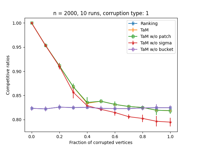
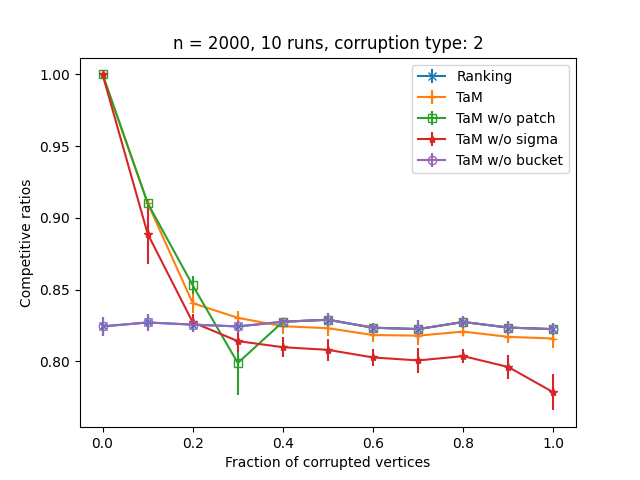
Figure 7: $n=2000$, averaged over 10 runs. TaM refers to our implementation of TestAndMatch.

In all cases, we see that the attained competitive ratio is highest when all extensions are enabled. We also see that the degradation below the baseline is not very severe ($<0.1$ for all cases, even when not all extensions are enabled).

Unsurprisingly, the competitive ratios of Ranking and “TaM without bucket” coincide because because $r/\varepsilon^{2}>n$ and we always default to baseline without performing any tests (to maintain robustness).

For corruption type 1, the “sigma remapping” extension makes our algorithm robust against additive edge corruption, and so the “patching” extension has no further impact.

References

- Aamand et al. (2022) Anders Aamand, Justin Chen, and Piotr Indyk. (Optimal) Online Bipartite Matching with Degree Information. Advances in Neural Information Processing Systems, 35:5724–5737, 2022.
- Alomrani et al. (2021) Mohammad Ali Alomrani, Reza Moravej, and Elias B Khalil. Deep policies for online bipartite matching: A reinforcement learning approach. arXiv preprint arXiv:2109.10380, 2021.
- Angelopoulos et al. (2020) Spyros Angelopoulos, Christoph Dürr, Shendan Jin, Shahin Kamali, and Marc Renault. Online Computation with Untrusted Advice. In 11th Innovations in Theoretical Computer Science Conference (ITCS 2020). Schloss Dagstuhl-Leibniz-Zentrum für Informatik, 2020.
- Antoniadis et al. (2020a) Antonios Antoniadis, Christian Coester, Marek Elias, Adam Polak, and Bertrand Simon. Online Metric Algorithms with Untrusted Predictions. In International Conference on Machine Learning, pages 345–355. PMLR, 2020a.
- Antoniadis et al. (2020b) Antonios Antoniadis, Themis Gouleakis, Pieter Kleer, and Pavel Kolev. Secretary and online matching problems with machine learned advice. Advances in Neural Information Processing Systems, 33:7933–7944, 2020b.
- Antoniadis et al. (2022) Antonios Antoniadis, Peyman Jabbarzade, and Golnoosh Shahkarami. A Novel Prediction Setup for Online Speed-Scaling. In 18th Scandinavian Symposium and Workshops on Algorithm Theory (SWAT 2022). Schloss Dagstuhl-Leibniz-Zentrum für Informatik, 2022.
- Bamas et al. (2020a) Étienne Bamas, Andreas Maggiori, Lars Rohwedder, and Ola Svensson. Learning Augmented Energy Minimization via Speed Scaling. Advances in Neural Information Processing Systems, 33:15350–15359, 2020a.
- Bamas et al. (2020b) Etienne Bamas, Andreas Maggiori, and Ola Svensson. The Primal-Dual method for Learning Augmented Algorithms. Advances in Neural Information Processing Systems, 33:20083–20094, 2020b.
- Bernardini et al. (2022) Giulia Bernardini, Alexander Lindermayr, Alberto Marchetti-Spaccamela, Nicole Megow, Leen Stougie, and Michelle Sweering. A Universal Error Measure for Input Predictions Applied to Online Graph Problems. In Advances in Neural Information Processing Systems, 2022.
- Birnbaum and Mathieu (2008) Benjamin Birnbaum and Claire Mathieu. On-line bipartite matching made simple. Acm Sigact News, 39(1):80–87, 2008.
- Borodin et al. (2020) Allan Borodin, Christodoulos Karavasilis, and Denis Pankratov. An experimental study of algorithms for online bipartite matching. Journal of Experimental Algorithmics (JEA), 25:1–37, 2020.
- Brubach et al. (2016) Brian Brubach, Karthik Abinav Sankararaman, Aravind Srinivasan, and Pan Xu. New algorithms, better bounds, and a novel model for online stochastic matching. In 24th Annual European Symposium on Algorithms (ESA 2016). Schloss Dagstuhl-Leibniz-Zentrum fuer Informatik, 2016.
- Brubach et al. (2020) Brian Brubach, Karthik Abinav Sankararaman, Aravind Srinivasan, and Pan Xu. Online stochastic matching: New algorithms and bounds. Algorithmica, 82(10):2737–2783, 2020.
- Canonne (2019) Clément L Canonne. A short note on poisson tail bounds. Available at http://www.cs.columbia.edu/ ccanonne/files/misc/2017-poissonconcentration.pdf, 2019.
- Chen et al. (2022) Justin Chen, Sandeep Silwal, Ali Vakilian, and Fred Zhang. Faster fundamental graph algorithms via learned predictions. In International Conference on Machine Learning, pages 3583–3602. PMLR, 2022.
- Choo et al. (2023) Davin Choo, Themistoklis Gouleakis, and Arnab Bhattacharyya. Active causal structure learning with advice. In International Conference on Machine Learning, pages 5838–5867. PMLR, 2023.
- Chung et al. (2003) Fan Chung, Linyuan Lu, and Van Vu. Spectra of random graphs with given expected degrees. Proceedings of the National Academy of Sciences, 100(11):6313–6318, 2003.
- Dinitz et al. (2021) Michael Dinitz, Sungjin Im, Thomas Lavastida, Benjamin Moseley, and Sergei Vassilvitskii. Faster matchings via learned duals. Advances in neural information processing systems, 34:10393–10406, 2021.
- Dinitz et al. (2022) Michael Dinitz, Sungjin Im, Thomas Lavastida, Benjamin Moseley, and Sergei Vassilvitskii. Algorithms with prediction portfolios. Advances in neural information processing systems, 35:20273–20286, 2022.
- Dütting et al. (2021) Paul Dütting, Silvio Lattanzi, Renato Paes Leme, and Sergei Vassilvitskii. Secretaries with Advice. In Proceedings of the 22nd ACM Conference on Economics and Computation, pages 409–429, 2021.
- Feldman et al. (2009) Jon Feldman, Aranyak Mehta, Vahab Mirrokni, and Shan Muthukrishnan. Online stochastic matching: Beating 1-1/e. In 2009 50th Annual IEEE Symposium on Foundations of Computer Science, pages 117–126. IEEE, 2009.
- Feng et al. (2021) Yiding Feng, Rad Niazadeh, and Amin Saberi. Two-stage stochastic matching with application to ride hailing. In Proceedings of the 2021 ACM-SIAM Symposium on Discrete Algorithms (SODA), pages 2862–2877. SIAM, 2021.
- Goel and Mehta (2008) Gagan Goel and Aranyak Mehta. Online budgeted matching in random input models with applications to Adwords. In SODA, volume 8, pages 982–991, 2008.
- Gollapudi and Panigrahi (2019) Sreenivas Gollapudi and Debmalya Panigrahi. Online Algorithms for Rent-or-Buy with Expert Advice. In International Conference on Machine Learning, pages 2319–2327. PMLR, 2019.
- Gouleakis et al. (2023) Themis Gouleakis, Konstantinos Lakis, and Golnoosh Shahkarami. Learning-Augmented Algorithms for Online TSP on the Line. In 37th AAAI Conference on Artificial Intelligence. AAAI, 2023.
- Han (2024) Yanjun Han. Personal communication (20 Jan 2024), 2024.
- Jaillet and Lu (2014) Patrick Jaillet and Xin Lu. Online stochastic matching: New algorithms with better bounds. Mathematics of Operations Research, 39(3):624–646, 2014.
- Jiao et al. (2018) Jiantao Jiao, Yanjun Han, and Tsachy Weissman. Minimax estimation of the {} distance. IEEE Transactions on Information Theory, 64(10):6672–6706, 2018.
- Jin and Ma (2022) Billy Jin and Will Ma. Online bipartite matching with advice: Tight robustness-consistency tradeoffs for the two-stage model. Advances in Neural Information Processing Systems, 35:14555–14567, 2022.
- Karande et al. (2011) Chinmay Karande, Aranyak Mehta, and Pushkar Tripathi. Online bipartite matching with unknown distributions. In Proceedings of the forty-third annual ACM symposium on Theory of computing, pages 587–596, 2011.
- Karp et al. (1990) Richard M Karp, Umesh V Vazirani, and Vijay V Vazirani. An optimal algorithm for on-line bipartite matching. In Proceedings of the twenty-second annual ACM symposium on Theory of computing, pages 352–358, 1990.
- Kraska et al. (2018) Tim Kraska, Alex Beutel, Ed H. Chi, Jeffrey Dean, and Neoklis Polyzotis. The Case for Learned Index Structures. In Proceedings of the 2018 international conference on management of data, pages 489–504, 2018.
- Lattanzi et al. (2020) Silvio Lattanzi, Thomas Lavastida, Benjamin Moseley, and Sergei Vassilvitskii. Online Scheduling via Learned Weights. In Proceedings of the Fourteenth Annual ACM-SIAM Symposium on Discrete Algorithms, pages 1859–1877. SIAM, 2020.
- Lavastida et al. (2020) Thomas Lavastida, Benjamin Moseley, R Ravi, and Chenyang Xu. Learnable and instance-robust predictions for online matching, flows and load balancing. arXiv preprint arXiv:2011.11743, 2020.
- Lavastida et al. (2021) Thomas Lavastida, Benjamin Moseley, R Ravi, and Chenyang Xu. Using predicted weights for ad delivery. In SIAM Conference on Applied and Computational Discrete Algorithms (ACDA21), pages 21–31. SIAM, 2021.
- Li et al. (2023) Pengfei Li, Jianyi Yang, and Shaolei Ren. Learning for edge-weighted online bipartite matching with robustness guarantees. In International Conference on Machine Learning, pages 20276–20295. PMLR, 2023.
- Lykouris and Vassilvitskii (2021) Thodoris Lykouris and Sergei Vassilvitskii. Competitive Caching with Machine Learned Advice. Journal of the ACM (JACM), 68(4):1–25, 2021.
- Mahdian and Yan (2011) Mohammad Mahdian and Qiqi Yan. Online Bipartite Matching with Random Arrivals: An Approach Based on Strongly Factor-Revealing LPs. In Proceedings of the forty-third annual ACM symposium on Theory of computing, pages 597–606, 2011.
- Manshadi et al. (2012) Vahideh H Manshadi, Shayan Oveis Gharan, and Amin Saberi. Online stochastic matching: Online actions based on offline statistics. Mathematics of Operations Research, 37(4):559–573, 2012.
- Mehta (2013) Aranyak Mehta. Online matching and ad allocation. Foundations and Trends® in Theoretical Computer Science, 8(4):265–368, 2013.
- Mitzenmacher (2018) Michael Mitzenmacher. A Model for Learned Bloom Filters, and Optimizing by Sandwiching. Advances in Neural Information Processing Systems, 31, 2018.
- Purohit et al. (2018) Manish Purohit, Zoya Svitkina, and Ravi Kumar. Improving Online Algorithms via ML Predictions. Advances in Neural Information Processing Systems, 31, 2018.
- Rohatgi (2020) Dhruv Rohatgi. Near-Optimal Bounds for Online Caching with Machine Learned Advice. In Proceedings of the Fourteenth Annual ACM-SIAM Symposium on Discrete Algorithms, pages 1834–1845. SIAM, 2020.
- Sakaue and Oki (2022) Shinsaku Sakaue and Taihei Oki. Discrete-convex-analysis-based framework for warm-starting algorithms with predictions. Advances in Neural Information Processing Systems, 35:20988–21000, 2022.
- Valiant and Valiant (2011) Gregory Valiant and Paul Valiant. The power of linear estimators. In 2011 IEEE 52nd Annual Symposium on Foundations of Computer Science, pages 403–412. IEEE, 2011.
- Valiant and Valiant (2017) Gregory Valiant and Paul Valiant. Estimating the unseen: improved estimators for entropy and other properties. Journal of the ACM (JACM), 64(6):1–41, 2017.
- Vazirani (2022) Vijay V Vazirani. Online Bipartite Matching and Adwords (Invited Talk). In 47th International Symposium on Mathematical Foundations of Computer Science (MFCS 2022). Schloss Dagstuhl-Leibniz-Zentrum für Informatik, 2022.
- Wang et al. (2020) Shufan Wang, Jian Li, and Shiqiang Wang. Online Algorithms for Multi-shop Ski Rental with Machine Learned Advice. Advances in Neural Information Processing Systems, 33:8150–8160, 2020.
- Wei (2020) Alexander Wei. Better and Simpler Learning-Augmented Online Caching. In Approximation, Randomization, and Combinatorial Optimization. Algorithms and Techniques (APPROX/RANDOM 2020). Schloss Dagstuhl-Leibniz-Zentrum für Informatik, 2020.
- Wu and Yang (2019) Yihong Wu and Pengkun Yang. Chebyshev polynomials, moment matching, and optimal estimation of the unseen. The Annals of Statistics, 47(2):857–883, 2019.