Size-Invariance Matters: Rethinking Metrics and Losses for
Imbalanced Multi-object Salient Object Detection

Abstract

This paper explores the size-invariance of evaluation metrics in Salient Object Detection (SOD), especially when multiple targets of diverse sizes co-exist in the same image. We observe that current metrics are size-sensitive, where larger objects are focused, and smaller ones tend to be ignored. We argue that the evaluation should be size-invariant because bias based on size is unjustified without additional semantic information. In pursuit of this, we propose a generic approach that evaluates each salient object separately and then combines the results, effectively alleviating the imbalance. We further develop an optimization framework tailored to this goal, achieving considerable improvements in detecting objects of different sizes. Theoretically, we provide evidence supporting the validity of our new metrics and present the generalization analysis of SOD. Extensive experiments demonstrate the effectiveness of our method. The code is available at https://github.com/Ferry-Li/SI-SOD.

1 Introduction

Salient object detection (SOD), also known as salient object segmentation, aims at highlighting visually salient regions in images  (Wang et al., 2022). To achieve this, a SOD model typically processes an RGB image to generate a binary mask, marking each pixel as either salient (1) or not (0). Recently, SOD has witnessed great progress in various applications (Mahadevan & Vasconcelos, 2009; Ren et al., 2014; Tang et al., 2017; Li et al., 2019; Zhang et al., 2020a; Jiang et al., 2023; Gui et al., 2024).

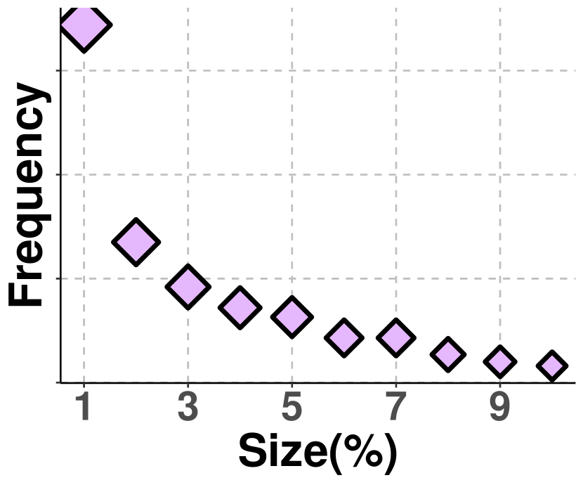
(a) Average size of objects

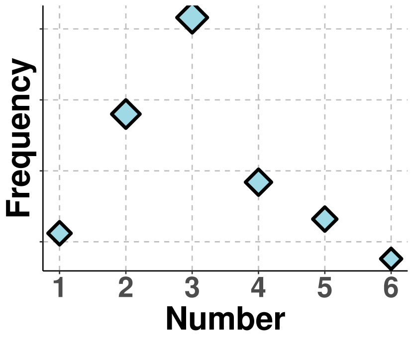
(b) Average number of objects

Figure 1: Statistics on dataset MSOD. Fig. 1(a) illustrates the widely existing small salient objects, with Size(%) as the proportion of the size of an object over the whole image.Fig. 1(b) reveals that practical SOD scenarios usually involve multiple salient objects.

The progress of SOD primarily depends on two factors. One is the development of sophisticated models (say deep neural networks), which effectively disentangle diverse feature patterns for accurate SOD detection. Notable methods include  (Wu et al., 2022; Luo et al., 2017; Wang et al., 2023; Ma et al., 2021; Zhang et al., 2021a). The other is the evaluation and selection of the best models for practical applications. Generally, a well-performed SOD model should simultaneously embrace a high True Positive Rate ($\mathsf{TPR}$) and a low False Positive Rate ($\mathsf{FPR}$) (Borji et al., 2019). To this end, various metrics (typically $\mathsf{MAE}$ and $\mathsf{F}$-score) have been widely considered for evaluation and optimization (Chen et al., 2021; Sun et al., 2022).

In this paper, we argue that current evaluation metrics are size-sensitive, which is not a proper choice for SOD tasks when the sizes of objects in a given image are highly imbalanced. As demonstrated in Fig. 1, SOD tasks typically involve multiple salient objects with diverse sizes. In this sense, prediction errors would be dominated by those larger objects, leading models to overlook small salient objects. Taking $\mathsf{MAE}$ as an example, Fig. 2(c) could merely detect the larger salient object but miss the smaller one on the right, while Fig. 2(d) could successfully capture all salient objects. However, Fig. 2(d) induces a worse $\mathsf{MAE}$ than Fig. 2(c), which is counter-intuitive to our visual perceptions. Large objects dominate size-sensitive metrics, consequently leading to practical performance degradation because there are many cases where small objects are critical for downstream tasks. For example, in a street view, traffic lights are usually of small size, but they play a significant role in autonomous driving tasks.

To address the issues above, we are interested in the following problem:

(a) Image

(b) Label

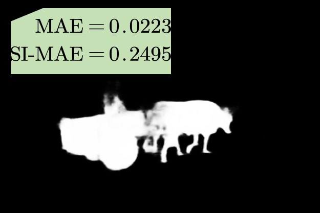
(c) EDN

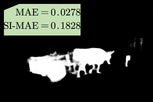
(d) EDN+Ours

Figure 2: (c) is the result of backbone EDN (Wu et al., 2022), and (d) is the prediction optimized by our approach. (c) detects fewer salient objects, yet enjoys lower $\mathsf{MAE}$ than (d). However, $\mathsf{SI\text{-}MAE}$ can correctly distinguish two detections.

The answer is affirmative in this paper. To begin with, we present a novel unified framework to understand why popular SOD metrics are size-sensitive. Specifically, given an image, we show that common criterion can be reformulated as a weighted (denoted by $\color[rgb]{0,0,1}{\mathbb{P}_{x_{i}}}$) sum of multiple independent parts, with each weighted term $\color[rgb]{0,0,1}{\mathbb{P}_{x_{i}}}$ being highly related to the size of the corresponding part. This creates an inductive bias toward objects of different sizes.

Motivated by this, we thus propose a simple yet effective paradigm for size-invariant SOD evaluation. The key idea is to modify the size-related term $\color[rgb]{0,0,1}{\mathbb{P}_{x_{i}}}$ into a size-invariant constant, ensuring equal treatment for each salient object regardless of size. Meanwhile, we introduce a generic Size-Invariant SOD (SI-SOD) optimization loss to pursue our size-invariant goal practically.

To show the effectiveness of our proposed paradigm, we then investigate the generalization performance of the SI-SOD algorithm. To the best of our knowledge, such a problem remains barely explored in the SOD community. As a result, we find that for composite losses (defined in Sec. 3.1), the size-invariant loss function leads to a sharper bound than its size-sensitive counterparts.

Finally, extensive experiments over a range of benchmark datasets speak to the efficacy of our proposed method.

2 Related Work

In recent years, SOD achieved considerable progress with elaborate frameworks and well-designed losses. We give a brief overview of SOD methods here and a detailed description of evaluation metrics in App. A.

Architecture-focused methods usually adopt convolutional networks as basic modules since their great success. For example, UCF (Zhang et al., 2017b) introduced a reformulated dropout after specific convolutional layers to learn deep uncertain convolutional features. DCL (Li & Yu, 2016) adopted a multi-stream framework, with the pixel-level fully convolutional stream to improve pixel-level accuracy. A common way to extract multi-level features is to design a bottom-up/top-down architecture, which resembles the U-Net (Ronneberger et al., 2015). PiCANet (Liu et al., 2018a) proposed a pixel-wise contextual attention network to selectively attend to informative context locations for each pixel and embed global and local networks into a U-Net architecture. RDCPN (Wu et al., 2021) introduced a novel multi-level ROIAlign-based decoder to adaptively aggregate multi-level features for better mask predictions. Similar structures are also utilized in recent works, including EDN (Wu et al., 2022), ICON (Zhuge et al., 2022), Bi-Directional (Zhang et al., 2018), CANet (Ren et al., 2021), etc.  (Piao et al., 2019) designed a refinement block to fully extract and fuse multi-scale features, successfully achieving excellent performance on most datasets. Based on this,  (Ji et al., 2022) further exploited a cascaded hierarchical feature fusion strategy to promote efficient information interaction of multi-level contextual features and efficiently improve contextual represent ability.

Multi-source-based methods have recently become popular. Specifically, both PoolNet (Liu et al., 2019) and MENet (Wang et al., 2023) conducted joint supervision of salient objects and object boundaries at each side-output.  (Ji et al., 2023) used thermal infrared images as extra input to deal with rainy, overexposure, or low-light occasions, and achieved effective results. Depth information is also widely used in SOD, which is usually named as RGB-D SOD. For instance, (Ji et al., 2020; Zhang et al., 2023; Li et al., 2023a, b) introduced depth map to SOD and significantly improved the detection performance. Furthermore,  (Zhang et al., 2019, 2020b) utilized light field data as an auxiliary for SOD and achieved state-of-the-art performance at that time. Some extensive works such as  (Zhang et al., 2021b; Ji et al., 2023; Li et al., 2023a) successfully deal with video SOD tasks exploiting the inter-frame information.

There are also previous works analyzing the evaluation in SOD.  (Bylinskii et al., 2019) provided a comprehensive analysis of eight different evaluation metrics and their properties.  (Borji et al., 2013a) performed a comparison of dozens of methods on many datasets to explore the consistency between the model ranking and practical performance. However, little attention has been paid to occasions where multiple salient objects co-exist, which is quiet common in the real world.

3 A Novel Size-invariant Evaluation Protocol

In this section, we begin by discussing why the commonly used metrics, such as Mean Absolute Error ($\mathsf{MAE}$) and $\mathsf{F}$-score, are not suitable for evaluating on imbalanced multi-object occasions. We then introduce methods to improve these metrics, aiming for a size-invariant SOD evaluation.

3.1 Revisiting Current SOD Evaluation Metrics

We start our analysis from standard functions, which could be divided into two groups: separable and composite functions, expressed as follows:

Definition 3.1 (Separable Function).

Given a predictor $f$, a function $g$ applied to $f$ is separable if the following equation formally holds: $$g(f(X),Y)=\sum_{i=1}^{n}w_{X_{i}}\cdot g(f(X_{i}),Y_{i}),$$ (1) with $$\bigcup_{i=1}^{n}X_{i}=X,\;\bigcap_{i=1}^{n}X_{i}=\varnothing,$$ (2) where $X$ is the input and $Y$ is the ground truth; $(X_{1},X_{2},\cdots,X_{n})$ are $n$ non-intersect parts of $X$; and $w_{X_{i}}$ is an $X_{i}$-related weight for the term $g(f(X_{i}),Y_{i})$.

According to the definition above, we realize that the point-wise evaluation metrics in the SOD community are separable (say Mean Absolute Error ($\mathsf{MAE}$) (Perazzi et al., 2012) and Mean Square Error ($\mathsf{MSE}$)).

Definition 3.2 (Composite Function).

Composite Functions are a series of compositions of separable functions Eq. 1, denoted by $\displaystyle G(f(X),Y)=(g_{1}\circ g_{2}\circ\dots\circ g_{T})\left(f(X),Y\right),$ where $T$ is the number of compositions. According to the definition above, complicated evaluation metrics such as $\mathsf{F}$-score (Achanta et al., 2009), $\mathsf{IOU}$ (Girshick et al., 2014) and $\mathsf{AUC}$ (Borji et al., 2013b) are composite. In what follows, we will discuss each of them respectively. For simplicity, we abbreviate $g(f(X),Y)$ and $G(f(X),Y)$ as $g(f)$ and $G(f)$ for a clear presentation.

Current separable metrics are NOT size-invariant. In SOD, the model $f:\mathbb{R}^{S}\to\mathbb{R}^{S}$ takes an image $X$ with label $Y$ as input, aiming to make a binary classification for each pixel, where $S$ is the size of the image and $Y=\{0,1\}^{S}$ is the pixel-level ground-truth. In light of this, the image could be naturally divided into $N_{c}$ parts based on the location of salient objects.

Therefore, given a certain separable SOD metric $g$, let $g(f_{i}):=g(f(X_{i}),Y_{i})$, we can rewrite it as Eq. 1 does:

$$g(f)=\sum_{i=1}^{N_{c}}{\color[rgb]{0,0,1}{\mathbb{P}_{X_{i}}}}\cdot g(f_{i}),$$ (3)

where $\mathbb{P}_{X_{i}}$ is the size-sensitive weight for the $i$-th part of $X$, which brings about inductive bias in evaluation.

Taking $\mathsf{MAE}$ as an example, the following equation holds:

$$\mathsf{MAE}(f) =\sum_{i=1}^{N_{c}}\frac{\|f(X_{i})-Y_{i}\|_{1,1}}{S}$$ (4)

$$=\sum_{i=1}^{N_{c}}\frac{S_{i}}{S}\cdot\frac{\|f(X_{i})-Y_{i}\|_{1,1}}{S_{i}}$$

$$=\sum_{i=1}^{N_{c}}\frac{S_{i}}{S}\cdot\mathsf{MAE}(f_{i})$$

$$=\sum_{i=1}^{N_{c}}{\color[rgb]{0,0,1}{\mathbb{P}_{X_{i}}}}\cdot\mathsf{MAE}(f_{i}).$$

Here we have $\color[rgb]{0,0,1}{\mathbb{P}_{X_{i}}=S_{i}/S}$, where $S_{i}$ represents the size of the $i$-th part. It is explicitly that the current $\mathsf{MAE}$ metric for SOD is size-sensitive, where larger objects would be paid more attention. Similar results can be drawn for other point-wise metrics in the SOD community.

Current composite metrics are NOT size-invariant. Similarly, we formally rewrite the composite metric $G(f)$ as follows:

$$G(f)=\frac{\sum_{i=1}^{N_{c}}{\color[rgb]{0,0,1}{\mathbb{P}_{X_{i}}}}(a_{1}g_{1}(f_{i})+\cdots+a_{T}g_{T}(f_{i}))}{\sum_{i=1}^{N_{c}}{\color[rgb]{0,0,1}{\mathbb{P}_{X_{i}}}}(b_{1}g_{1}(f_{i})+\cdots+b_{T}g_{T}(f_{i}))},$$ (5)

where again $g_{t}(f_{i}):=g_{t}(f(X_{i}),Y_{i}),t\in[T]$ is a certain separable metric value over the $i$-th part $X_{i}$; $a_{i}$ and $b_{i}$ represent coefficients for different composite functions, and here $\mathbb{P}_{X_{i}}$ is also a size-sensitive weight for each separable part of $X$.

Specifically, in terms of the widely used $\mathsf{F}$-score (Achanta et al., 2009), we have:

$$\mathsf{F}(f)=\frac{2\sum_{i=1}^{N_{c}}\mathsf{TP}(f_{i})}{\sum_{i=1}^{N_{c}}[2\mathsf{TP}(f_{i})+\mathsf{FP}(f_{i})+\mathsf{FN}(f_{i})]}$$ (6)

$$=\frac{2\sum_{i=1}^{N_{c}}\frac{S_{i}}{S}\cdot\frac{\mathsf{TP}(f_{i})}{S_{i}}}{\sum_{i=1}^{N_{c}}[\frac{S_{i}}{S}\cdot(2\frac{\mathsf{TP}(f_{i})}{S_{i}}+\frac{\mathsf{FP}(f_{i})}{S_{i}}+\frac{\mathsf{FN}(f_{i})}{S_{i}})]}$$

$$=\frac{2\sum_{i=1}^{N_{c}}{\color[rgb]{0,0,1}{\mathbb{P}_{X_{i}}}}\cdot\mathsf{TPR}(f_{i})}{\sum_{i=1}^{N_{c}}{\color[rgb]{0,0,1}{\mathbb{P}_{X_{i}}}}\cdot(2\mathsf{TPR}(f_{i})+\mathsf{FPR}(f_{i})+\mathsf{FNR}(f_{i}))},$$

where $\mathsf{TP}(f_{i})$, $\mathsf{FP}(f_{i})$, $\mathsf{FN}(f_{i})$ represent the number of True Positives, False Positives and False Negatives within $X_{i}$, and $\mathsf{TPR}(f_{i}),\mathsf{FPR}(f_{i}),\mathsf{FNR}(f_{i})$ represent the corresponding True Positive Rate, False Positive Rate, and False Negative Rate, which are all separable functions mentioned above. In this case, we still have $\color[rgb]{0,0,1}{\mathbb{P}_{X_{i}}=S_{i}/S}$, which is sensitive to the size of salient objects. Similar conclusion also applies to metrics like $\mathsf{AUC}$, with analysis in LABEL:wAUC_metric.

Why size-invariance MATTERS? We have realized that the existing widely adopted metrics would inevitably introduce biased weights for objects of different sizes. With this imbalance, smaller objects are suppressed by larger ones, and therefore are easily ignored in both evaluation and prediction. Unfortunately, as shown in Fig. 1, practical SOD tasks usually involve multiple objects of various sizes, including small yet critical ones. For example, Fig. 2(c) totally overlooks a small object, but enjoys a similar $\mathsf{MAE}$ compared to Fig. 2(d), which contradicts our visual perceptions. To rectify this, we introduce the principles of size-invariant evaluation in the next section.

3.2 Principles of Size-Invariant Evaluation

Based on the discussions above, the fundamental limitation of the current evaluation lies in the size-sensitive $\color[rgb]{0,0,1}{\mathbb{P}_{X_{i}}}$. Therefore, a principal way to achieve size-invariant evaluation is to eliminate the effect of the weighting term $\color[rgb]{0,0,1}{\mathbb{P}_{X_{i}}}$. In this paper, we propose a simple yet effective size-invariant protocol:

$$g_{\mathsf{SI}}(f)=\frac{1}{N_{c}}\sum_{i=1}^{N_{c}}{\color[rgb]{1,.5,0}{1}}\cdot g(f_{i}),$$ (7)

$$G_{\mathsf{SI}}(f)=\frac{1}{N_{c}}\sum_{i=1}^{N_{c}}{\color[rgb]{1,.5,0}{1}}\cdot\frac{(a_{1}g_{1}(f_{i})+\cdots+a_{T}g_{T}(f_{i}))}{(b_{1}g_{1}(f_{i})+\cdots+b_{T}g_{T}(f_{i}))},$$ (8)

where $\color[rgb]{0,0,1}{\mathbb{P}_{X_{i}}}$ is replaced by a constant $\color[rgb]{1,.5,0}{1}$. The size-sensitive weight is directly eliminated, and we naturally arrive at size-invariance.

In what follows, we will adopt widely used metrics, i.e., $\mathsf{MAE}$, $\mathsf{F}$-score and $\mathsf{AUC}$, to instantiate our size-invariant principles. Note that our proposed strategy could also be applied to other metrics as mentioned in Sec. 4.

3.2.1 Size-Invariant $\mathsf{MAE}$

According to Eq. 7, $\mathsf{SI\text{-}MAE}$ is expressed as follows:

$$\mathsf{SI\text{-}MAE}(f)=\frac{1}{N_{c}}\sum_{i=1}^{N_{c}}{\color[rgb]{1,.5,0}{1}}\cdot\mathsf{MAE}(f_{i}).$$ (9)

Here our primary focus is on dividing the image into $N_{c}$ parts. Motivated by the success of object detection (Ren et al., 2015) (Redmon et al., 2016), we segment salient objects into a series of foreground frames by their minimum bounding boxes, and pixels that do not form part of any bounding box are treated as the background.

Ideally, assume that there are $K$ salient objects in an image and let $C_{k}=\{(a_{j},b_{j})\}_{j=1}^{M_{k}},k\in[K]$ be the coordinate set for the object $k$, then the minimum bounding box for object $k$ could be determined clockwise by the following vertex coordinates:

$$X_{k}^{fore}= \{(a_{k}^{min},b_{k}^{max}),(a_{k}^{max},b_{k}^{max}),$$ (10)

$$(a_{k}^{max},b_{k}^{min}),(a_{k}^{min},b_{k}^{min})\},$$

where $a_{k}^{min},a_{k}^{max},b_{k}^{min},b_{k}^{max}$ are the minimum and maximum coordinates in $C_{k}$, respectively.

Correspondingly, the background frame is defined as follows:

$$X^{back}_{K+1}=X\setminus F,$$ (11)

where

$$F=\bigcup_{k=1}^{K}X_{k}^{fore}$$ (12)

is the collection of all minimum bounding boxes for salient objects.

However, since there is no instance-level label to distinguish different objects in most practical datasets, we instead regard each connected component composed of salient objects in the saliency map as an independent proxy $C_{k}$. Some examples of partitions are presented in Fig. 3, where an image will be divided into $N_{c}=K+1$ parts, including $K$ foreground frames and a background frame. Please refer to implementation details in Sec. 5.1 for more details of the connected component.

The bounding boxes are similar to those widely applied in the area of object detection (Xiao & Marlet, 2020) (Ding et al., 2022). However, object detection makes bounding box regression to match the predicted boxes as close to the ground-truth boxes as possible, while our approach generates the bounding boxes from the ground-truth binary masks and exploits them as auxiliary tools to calculate the loss and metric results around each salient object.

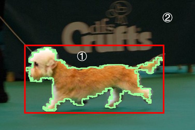
(a) Single-object scenario

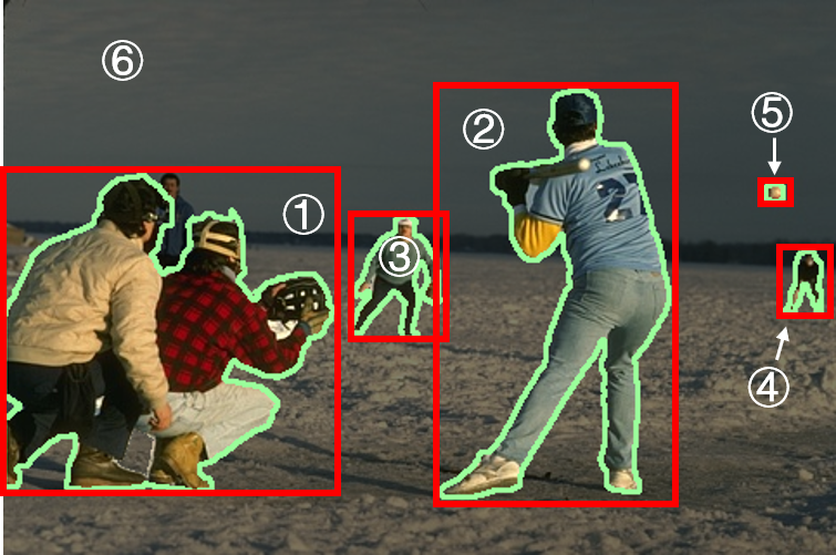
(b) Multi-object scenario

Figure 3: Examples of partitions. In Fig. 3(a), there is a foreground frame ➀ and a background frame ➁. In Fig. 3(b), there are five foreground frames from ➀ to ➄, and a background frame ➅.

In this way, the goal of $\mathsf{SI\text{-}MAE}$ becomes

$$\mathsf{SI\text{-}MAE}(f) =$$ (13)

$$\frac{1}{K+\alpha} \left[\sum_{k=1}^{K}\mathsf{MAE}(f_{k}^{fore})+\alpha\mathsf{MAE}(f_{K+1}^{back})\right],$$

where a parameter $\alpha$, determined by the ratio of the size of the background and the sum of all foreground frames, namely $\alpha=\frac{S_{K+1}^{back}}{\sum_{k=1}^{K}S_{k}^{fore}}$, is further introduced to balance the model attention adaptively. By doing so, the predictor could not only pay equal consideration to salient objects of various sizes, but also impose an appropriate penalty for misclassifications in the background. This plays an important role in reducing the false positives as illustrated in Sec. 5.3.3.

In the following, we make a brief discussion between $\mathsf{MAE}$ and our proposed $\mathsf{SI\text{-}MAE}$, with proof in LABEL:prop1_proof.

Proposition 3.3 (Informal).

Given two different predictors $f_{A}$ and $f_{B}$, the following two possible cases suggest that $\mathsf{SI\text{-}MAE}$ is more effective than $\mathsf{MAE}$ during evaluation. Case 1: Assume that there is a single salient object (i.e., $K=1$), with two different results from predictors $f_{A}$ and $f_{B}$. In this case, there is no imbalance from different sizes of objects, and therefore $\mathsf{SI\text{-}MAE}$ is equivalent to $\mathsf{MAE}$. Case 2: Suppose there are two salient objects ($K=2$) where $f_{A}$ and $f_{B}$ detect the same amount of salient pixels in an image $X$. Meanwhile, assume that $f_{A}$ only predicts $C_{2}$ perfectly while $f_{B}$ could somewhat recognize $C_{1}$ and $C_{2}$ partially. In this case, $f_{B}$ should still be better than $f_{A}$ since $f_{A}$ totally fails on $C_{1}$. Unfortunately, if $S_{1}^{fore}<S_{2}^{fore}$, $\mathsf{MAE}(f_{A})=\mathsf{MAE}(f_{B})$ holds but we have $\mathsf{SI\text{-}MAE}(f_{A})>\mathsf{SI\text{-}MAE}(f_{B})$.

Remark. Fig. 2 provides a toy example for Case 2. Discussions above support that $\mathsf{MAE}$ is sensitive to the size of objects concerning multiple object cases, yet $\mathsf{SI\text{-}MAE}$ can serve our expectations better. We also extend our analysis to the case with $K\geq 3$, which consistently suggests the efficacy of $\mathsf{SI\text{-}MAE}$. The detailed discussion is attached to LABEL:prop1_proof.

3.2.2 Size-Invariant Composite Metrics

Here we instantiate our size-invariant principle with common composite metrics, including $\mathsf{F}$-score and $\mathsf{AUC}$.

As to the composite metric $\mathsf{F}$-score, we define $\mathsf{SI\text{-}F}$ as follows:

$$\mathsf{SI\text{-}F}(f)=\frac{1}{K}\sum_{i=1}^{K}\mathsf{F}(f_{k}^{fore}),$$ (14)

where $X_{1}^{fore},\cdots,X_{K}^{fore}$ denote foreground frames. Similar to $\mathsf{SI\text{-}MAE}$, we give a proposition in App. B to support that in multiple object cases, $\mathsf{SI\text{-}F}$ can serve our expectations better.

As to another common composite metric $\mathsf{AUC}$, we similarly define $\mathsf{SI\text{-}AUC}$ as follows:

$$\mathsf{SI\text{-}AUC}(f)=\frac{1}{K}\sum_{i=1}^{K}\mathsf{AUC}(f_{k}^{fore}),$$ (15)

where $X_{1}^{fore},\cdots,X_{K}^{fore}$ denote foreground frames. The analysis of $\mathsf{SI\text{-}AUC}$ is deferred to LABEL:wAUC_metric due to space limitations.

4 How to Practically Pursue Size-Invariance?

In previous sections, we outlined how to achieve size-invariant evaluation for SOD. Now this section explores how to directly optimize these size-invariant metrics to promote practical SOD performance.

4.1 A Generic Size-Invariant Optimization Goal

Motivated by the principles of the size-invariant evaluation, our optimization goal is expressed as follows:

$$\mathcal{L}_{\mathsf{SI}}(f)=\sum_{k=1}^{K}\ell(f_{k}^{fore})+\alpha\ell(f_{K+1}^{back}),$$ (16)

where $\ell(\cdot)$ could be any popular loss in the SOD community (such as $\mathsf{BCE}$ or $\mathsf{IOU}$). For simplicity, we let $\ell(f):=\ell(f(X),Y)$ and $\ell(f_{i}):=\ell(f(X_{i}),Y_{i})$. Similar to Eq. 13, if $\ell(\cdot)$ is separable, we set $\alpha=\frac{S^{back}_{K+1}}{\sum_{k=1}^{K}S_{k}^{fore}}$; for composite losses like DiceLoss (Milletari et al., 2016) and IOU Loss (Yu et al., 2016), we set $\alpha=0$ because the $\mathsf{TPR}$ is always 0 in the background. Specifically in LABEL:loss_description, we describe detailed implementations of Size-Invariant Optimization for different backbones discussed in Sec. 5.

As discussed in Sec. 3.2, Eq. 16 ensures that the model treats all objects equally regardless of size, thus improving the detection of smaller objects. We give the following proposition to illustrate the mechanism of SI-SOD, with proof in LABEL:re-attention_proof.

Proposition 4.1 (Mechanism of SI-SOD).

Given a separable loss function $\ell(\cdot)$ and its corresponding size-invariant loss $\mathcal{L}_{\mathsf{SI}}(\cdot)$, then for a certain scenario: 1. when $S_{i}<\frac{S}{K+\alpha}$, we have $w_{\mathcal{L}_{\mathsf{SI}}}(x_{i})>w_{\ell}(x_{i})$, 2. when $S_{i}<S_{j},$ we have $w_{\mathcal{L}_{\mathsf{SI}}}(x_{i})>w_{\mathcal{L}_{\mathsf{SI}}}(x_{j})$. where $w_{\mathcal{L}_{\mathsf{SI}}}(x_{i})$ is the weight of pixel-level loss in $X_{i}$ with $\mathcal{L}_{\mathsf{SI}}$, and $w_{\ell}(x_{i})$ is the weight of pixel-level loss in $X_{i}$ with the original loss $\ell$. Remark. Compared to standard losses such as $\mathsf{BCE}$, SI-SOD adaptively adjusts the weight of pixel-level loss to ensure equal treatment on different objects.

Item 1 illustrates that smaller objects, which fall below a certain size threshold, will produce more loss. Item 2 describes that SI-SOD increases the weight for pixels in smaller salient objects, finally alleviating size-sensitivity.

4.2 Generalization Bound

In this section, we theoretically demonstrate that SI-SOD can generalize to common SOD tasks, despite several challenges.

First, SOD is considered as structured prediction (Ciliberto et al., 2020; Li et al., 2021), where couplings between output substructures make it difficult to directly apply Rademacher Complexity-based techniques in theoretical analysis. The standard result to bound the empirical Rademacher complexity (Michel Ledoux, 1991) holds when the prediction functions are real-valued. To overcome this, we adopt the vector contraction inequality (Maurer, 2016) to extend it from real-valued analysis to vector-valued ones, and consequently reach a sharper result with Lipschitz properties (Foster & Rakhlin, 2019).

Another challenge lies in the diversity of losses, which hinders exploring the generalization properties within a coordinated framework. Therefore, by studying from the view of separable and composite functions respectively, we obtain Lipschitz properties (Dembczyński et al., 2017) for both categories and ultimately achieve a unified conclusion.

We present our conclusions here, and the proof is deferred to LABEL:generalization_bound_proof.

Theorem 4.2 (Generalization Bound for SI-SOD).

Assume $\mathcal{F}\subseteq\{f:\mathcal{X}\to\mathbb{R}^{K}\}$, where $K=H\times W$ is the pixel count in an image, $g^{(i)}$ is the risk over $i$-th sample, and is $L$-Lipschitz with respect to the $l_{\infty}$ norm, (i.e. $\|g(x)-g(\tilde{x})\|_{\infty}\leq L\cdot\|x-y\|_{\infty}$). When there are $N$ $i.i.d.$ samples, there exists a constant $C>0$ for any $\epsilon>0$, the following generalization bound holds with probability at least $1-\delta$: $\displaystyle~{}\sup_{f\in\mathcal{F}}(\mathbb{E}[g(f)]-\hat{\mathbb{E}}[g(f)])$ (17) $\displaystyle\leq$ $\displaystyle~{}C\cdot\frac{L\sqrt{K}}{N}\cdot\max_{i}\mathfrak{R}_{N}(\mathcal{F}|_{i})\cdot\log^{\frac{3}{2}+\epsilon}\left(\frac{N}{\max_{i}\mathfrak{R}_{N}(\mathcal{F}|_{i})}\right)$ $\displaystyle+3\sqrt{\frac{\log\frac{2}{\delta}}{2N}},$ where again $g(f(X,Y)):=g(f)$, $\mathbb{E}[g(f)]$ and $\hat{\mathbb{E}}[g(f)]$ represent the expected risk and empirical risk. $\mathfrak{R}_{N}(\mathcal{F};x_{1:N})=\max_{x_{1:N}\in\mathcal{X}}\mathfrak{R}(\mathcal{F};x_{1:N})$ denotes the worst-case Rademacher complexity, and we let $\mathfrak{R}_{N}(\mathcal{F}|i)$ denote its restriction to output coordinate $i$. Specifically, Case 1: For separable loss functions $\ell(\cdot)$, if it is $\mu$-Lipschitz, we have $L=\mu$. Case 2: For composite loss functions, when $\ell(\cdot)$ is DiceLoss (Milletari et al., 2016), we have $L=\frac{4}{\rho}$, where $\rho=\min\frac{S_{l}^{1,i}}{S_{l}^{i}}$, which represents the minimum proportion of the salient object in the $l$-th frame within the $i$-th sample. Remark. We reach a bound of $\mathcal{O}(\frac{\sqrt{K}\log N}{N})$, which indicates reliable generalization with a large training set.

Specifically, for case 2, the original composite loss $\ell(\cdot)$, still taking DiceLoss as an example, will result in a $\rho^{\prime}=\frac{S^{1,i}}{S^{i}}$, which represents the proportion of salient pixels in an image. It is obvious that $\rho>\rho^{\prime}$ because SI-SOD enlarges the proportion by reducing the denominator from the whole image to a bounding box, and finally leads to a smaller $L$ and a sharper bound.

Table 1: Quantitative comparisons on MSOD and DUTS-TE. The better results are shown with bold, and darker color indicates superior results. Metrics with $\uparrow$ mean higher value represents better performance, while $\downarrow$ mean lower value represents better performance.

Dataset	Methods	$\mathsf{MAE}\downarrow$	$\mathsf{SI\text{-}MAE}\downarrow$	$\mathsf{AUC}\uparrow$	$\mathsf{SI\text{-}AUC}\uparrow$	$\mathsf{F}_{m}^{\beta}\uparrow$	$\mathsf{SI\text{-}F}_{m}^{\beta}\uparrow$	$\mathsf{F}_{max}^{\beta}\uparrow$	$\mathsf{SI\text{-}F}_{max}^{\beta}\uparrow$	$\mathsf{E}_{m}\uparrow$
MSOD	PoolNet	0.0752	0.1196	0.9375	0.9563	0.6645	0.6397	0.7755	0.8402	0.7529
	+ Ours	0.0635	0.0924	0.9553	0.9721	0.7314	0.7467	0.8200	0.8867	0.8286
	LDF	0.0508	0.0946	0.8719	0.9246	0.7589	0.6691	0.8144	0.7575	0.8241
	+ Ours	0.0506	0.0893	0.9530	0.9441	0.7796	0.7573	0.8415	0.8879	0.8726
	ICON	0.0545	0.0945	0.8973	0.8909	0.7687	0.7029	0.8178	0.7789	0.8487
	+ Ours	0.0535	0.0830	0.9537	0.9514	0.7691	0.7738	0.8373	0.8665	0.8742
	GateNet	0.0442	0.0808	0.9331	0.9244	0.8005	0.7581	0.8510	0.8434	0.8776
	+ Ours	0.0444	0.0734	0.9456	0.9436	0.8157	0.8083	0.8570	0.8724	0.8972
	EDN	0.0467	0.0788	0.9196	0.9188	0.7925	0.7635	0.8410	0.8321	0.8712
	+ Ours	0.0453	0.0724	0.9401	0.9387	0.8057	0.7990	0.8555	0.8619	0.8936
DUTS-TE	PoolNet	0.0656	0.0609	0.9607	0.9716	0.7200	0.7569	0.8245	0.8715	0.8103
	+ Ours	0.0621	0.0562	0.9706	0.9824	0.7479	0.8172	0.8438	0.9029	0.8478
	LDF	0.0419	0.0410	0.9337	0.9680	0.8203	0.8201	0.8735	0.8802	0.8821
	+ Ours	0.0440	0.0422	0.9690	0.9756	0.8076	0.8388	0.8736	0.9117	0.8895
	ICON	0.0461	0.0454	0.9469	0.9424	0.8131	0.8270	0.8648	0.8815	0.8858
	+ Ours	0.0454	0.0435	0.9640	0.9706	0.8031	0.8395	0.8629	0.8958	0.8921
	GateNet	0.0383	0.0380	0.9629	0.9619	0.8292	0.8519	0.8835	0.9041	0.9053
	+ Ours	0.0399	0.0375	0.9663	0.9692	0.8185	0.8687	0.8743	0.9116	0.9038
	EDN	0.0389	0.0388	0.9600	0.9611	0.8288	0.8565	0.8752	0.9017	0.9033
	+ Ours	0.0392	0.0381	0.9658	0.9687	0.8260	0.8672	0.8765	0.9119	0.9072

5 Experiments

In this section, we describe some details of the experiments and present our results. Due to space limitations, please refer to LABEL:Experiments_appendix for an extended version.

5.1 Experimental Setups

Datasets. Eight datasets, DUTS (Wang et al., 2017), ECSSD (Yan et al., 2013), DUT-OMRON (Yang et al., 2013), HKU-IS (Li & Yu, 2015), MSOD (Deng et al., 2023), PASCAL-S (Yan et al., 2013), SOD (Movahedi & Elder, 2010) and XPIE (Xia et al., 2017), are included in the experiment. Following common practice, we train our network on the DUTS training set (DUTS-TR) and test it on the DUTS test set (DUTS-TE) and the other seven datasets. Detailed introductions on these datasets are deferred to LABEL:dataset_appendix.

Competitors. To demonstrate the effectiveness of size-invariant loss, we integrate it into five state-of-the-art backbones: EDN (Wu et al., 2022), ICON (Zhuge et al., 2022), GateNet (Zhao et al., 2020), LDF (Wei et al., 2020), PoolNet (Liu et al., 2019). EDN, ICON, and LDF utilize DiceLoss or IOULoss to handle the potential imbalanced distribution, and ICON specifically focuses on the macro-integrity, which are summarized at LABEL:competitor_appendix with details. Specifically, we modify the original loss functions into their corresponding size-invariant versions following Eq. 16, and re-train the network with the same setting. Correspondingly, we also compare the time cost of our method with original optimization frameworks, which is deferred at LABEL:time_cost.

Evaluation Metrics. Apart from our proposed metrics $\mathsf{SI\text{-}MAE}$, $\mathsf{SI\text{-}F}$ and $\mathsf{SI\text{-}AUC}$, we also include common metrics such as Mean Absolute Error($\mathsf{MAE}$), max F-measure($\mathsf{F}_{max}^{\beta}$), mean F-measure($\mathsf{F}_{m}^{\beta}$) and $\mathsf{AUC}$.

Another widely used metric is $\mathsf{E}_{m}$ introduced by (Fan et al., 2018), which is a newly proposed metric considering both global and local information. Definitions and calculations of all metrics are deferred to App. A.

Implementation Details. We carried out the experiments on a single GeForce RTX 3090. To ensure fairness, both the original and modified backbones are trained under identical settings. All images are resized into $384\times 384$ for training and testing, and the ResNet50 (He et al., 2016) pre-trained on ImageNet (Deng et al., 2009) is loaded. Specific settings and optimization details for each backbone are deferred at LABEL:details_appendix and LABEL:loss_description.

We preprocess the dataset with the package skimage, which identifies connected components with the ground-truth mask. Then we obtain the minimum bounding box following Eq. 10. Note that all procedures can also be done during training without any preprocessing.

5.2 Overall Performance

As mentioned above, we re-train the backbones with our size-invariant loss for a fair comparison. Tab. 1 shows the results on MSOD and DUTS-TE. The result is shown in a pair of backbones before and after applying our size-invariant loss, with the superior result highlighted in bold.

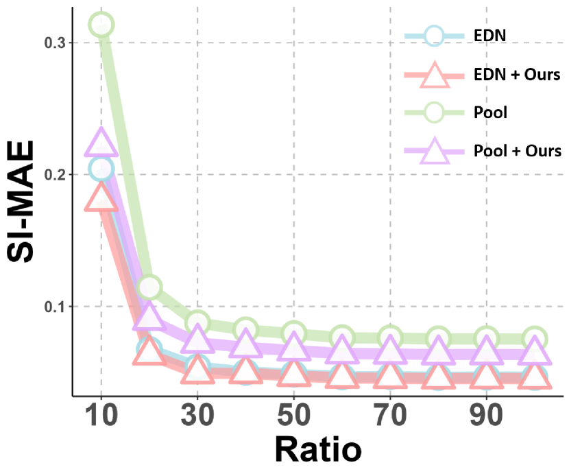
(a) MSOD

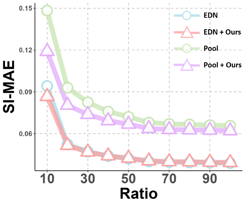
(b) DUTS

Figure 4: $\mathsf{SI\text{-}MAE}$ performance on objects with different sizes on two representative datasets, with EDN and PoolNet as backbones.

Since samples in MSOD contain multiple salient objects, it naturally arises that small objects can be overlooked due to the imbalance. Therefore, all backbones with our loss achieve considerable improvements on nearly all metrics, even including the original $\mathsf{MAE}$. Averagely, our method outperforms other frameworks by around 0.012, 0.038, 0.070, 0.065, 0.038 on $\mathsf{SI\text{-}MAE}$, $\mathsf{SI\text{-}AUC}$, $\mathsf{SI\text{-}F}_{m}^{\beta}$, $\mathsf{SI\text{-}F}_{max}^{\beta}$ and $\mathsf{E}_{m}$, respectively.

Tab. 1 also shows the performance on DUTS-TE. Our method achieves better results on almost all size-invariant metrics and $\mathsf{E}_{m}$, and stays competitive in terms of original $\mathsf{MAE}$ and $\mathsf{F}$-score. This justifies that the size-invariant loss achieves similar performance on single-object scenarios, suggesting the superior generalization ability of our loss. Averagely, our method outperforms other frameworks by around 0.001, 0.012, 0.024, 0.020, 0.011 on $\mathsf{SI\text{-}MAE}$, $\mathsf{SI\text{-}AUC}$, $\mathsf{SI\text{-}F}_{m}$, $\mathsf{SI\text{-}F}_{max}^{\beta}$, $\mathsf{E}_{m}$ on DUTS-TE. Results on other datasets are deferred to LABEL:tab:exp_result_appendix.

Fig. 6 shows the qualitative comparison on different backbones. While the original backbones may fail to detect all the salient objects in some hard samples, our method can significantly improve the detection on multi-object occasions. For example, in the 1st image, EDN only finds the largest sailboat on the right but fails to detect two smaller targets on the left, while ours additionally detects two small sailboats. In the 4th image, EDN detects fewer false positive pixels and ICON detects one more salient object with our loss. In the 3rd, 5th, and 6th images, all backbones detect more salient objects at the right part after using our loss. More qualitative comparisons are deferred to LABEL:Qualitative_appendix.

5.3 Fine-grained Analysis

5.3.1 Performance with Respect to Sizes

We conduct size-relevant analysis on five datasets. As it is the size of salient objects that our method focuses on, we divide all salient objects into ten groups according to their proportion to the entire image, ranging from [0%, 10%], [10%,20%], and finally up to [90%, 100%]. We evaluate the performance within each group, and here we only take foreground frames into account to concentrate on the detection performance of salient objects with different sizes.

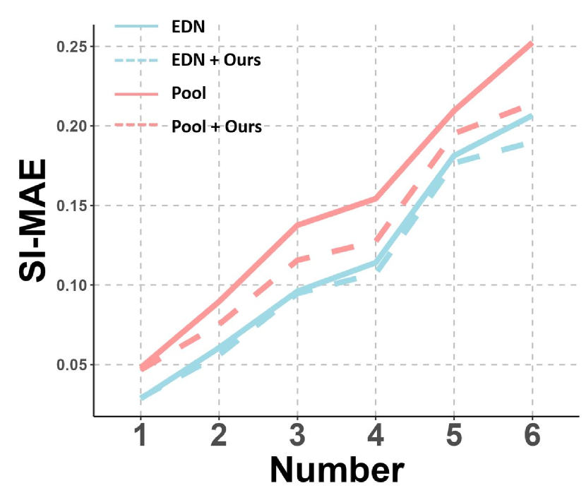
(a) MSOD

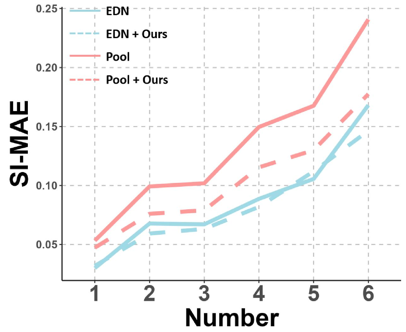
(b) DUTS

Figure 5: $\mathsf{SI\text{-}MAE}$ performance with different object numbers on two representative datasets, with EDN and PoolNet as backbones.

From Fig. 4, we observe that all backbones perform well on larger objects but show remarkable improvements on smaller objects when using our method. This aligns with our objective to enhance the detection of smaller objects. Specifically, for objects with size in [0%, 10%] of the image, our method outperforms the previous backbone, say EDN, by around 0.024 on $\mathsf{SI\text{-}MAE}$ on the MSOD dataset. As seen in Fig. 1(a), small-size salient objects usually account for the majority, therefore such improvement firmly speaks to our progress. This is not reflected by size-sensitive metrics like $\mathsf{MAE}$, but can be directly revealed by our proposed $\mathsf{SI\text{-}MAE}$. Performance analysis with respect to the object size on other backbones and datasets is deferred to LABEL:size-fine-grained_appendix.

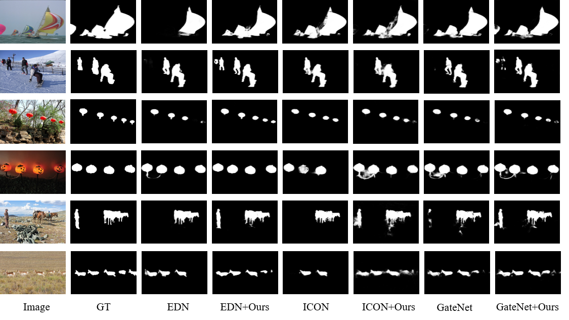
Figure 6: Qualitative comparison on different backbones.

5.3.2 Performance with Respect to Object Numbers

We also conduct number-relevant analysis on five datasets to evaluate the performance on single-object and multi-object scenarios, as shown in Fig. 5. With the number of salient objects increasing, the SOD tasks are getting imbalanced, where some objects are more likely to be ignored. Therefore, we divide all samples into several groups according to the number of salient objects in the image.

Generally, our method shows substantial improvements in multi-object scenarios and remains competitive in single-object cases, which again justifies the generalization and universality of our method. Specifically, for samples with greater than or equal to two salient objects, EDN gains an improvement by around 0.007 on $\mathsf{SI\text{-}MAE}$ on the MSOD dataset after employing our size-invariant loss. Performance analysis with respect to the object numbers on other backbones and datasets is deferred to LABEL:number-fine-grained_appendix.

(a) MSOD

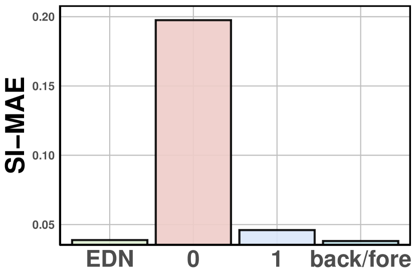
(b) DUTS

Figure 7: $\mathsf{SI\text{-}MAE}$ performance on two representative datasets with different value of $\alpha$. EDN, 0, 1, and back/fore represent the original backbone EDN, $\alpha=0$, $\alpha=1$ and $\alpha=\frac{S^{back}}{S^{fore}}$, respectively.

5.3.3 Ablation Studies

To investigate how the parameter $\alpha$ works, we conduct ablation studies on $\alpha$ to verify its effectiveness. Here we set $\alpha$ among $0,1,\frac{S^{back}}{S^{fore}}$. $\alpha=0$ indicates that we do not consider the background frame and pay all attention to foreground frames, while $\alpha=1$ means that we consider the background frame equally as other foreground frames, and $\alpha=\frac{S^{back}}{S^{fore}}$ is exactly our method. Fig. 7 illustrates the ablations on dataset MSOD and DUTS with the backbone EDN. $\alpha=0$ induces an extreme result with a high score within foreground frames and a low score in the background frame because it solely focuses on foreground detection. $\alpha=1$ alleviates the phenomenon, and surpasses the original framework on some metrics, but still predicts too many false positives, due to the slight penalty on the error within the background frame. Experiments on other datasets also speak to the efficacy of the $\alpha$. More detailed results are deferred to LABEL:ablation_appendix.

6 Conclusion

In this paper, we explore the size-invariance in SOD tasks. When multiple objects of various sizes co-exist, we observe that current evaluation metrics are size-sensitive, where larger objects are focused and smaller objects are likely overlooked. To rectify this, we introduce a generic approach to achieve size-invariance. Specifically, we propose $\mathsf{SI\text{-}MAE}$ and $\mathsf{SI\text{-}F}$, which evaluate each salient object separately before merging their results. We further design an optimization framework directly toward this goal, which can adaptively balance the weights to ensure equal treatment on different objects. Theoretically, we provide evidence to support our proposed metrics and present the generalization analysis for our SI-SOD optimization loss. Comprehensive experiments consistently demonstrate the efficacy of our method.

Impact Statement

We propose a general SOD method to deal with the potential bias toward small objects. For fairness-sensitive scenarios, it might be helpful to improve fairness for minority groups.

dasdsa

Contents

section[0em].

subsection[1.5em]. *[0.75em].

[sections]

[sections]l1

Appendix A Evaluation Metrics for SOD

Different from usual classification tasks where we calculate accuracy on the image level, SOD requires evaluation pixel by pixel. Other pixel-level tasks like semantic segmentation adopt $\mathsf{mIOU}$, which utilizes the mean $\mathsf{IOU}$ over all classes as the metric. However, in SOD all salient objects are labeled with 1 without further class labels. Therefore, there is no representative metric, and the following are commonly utilized:

$\mathsf{MAE}$ (Perazzi et al., 2012). It measures the average absolute error pixel-wise. The prediction is normalized to $[0,1]$ when calculating the errors from the ground truth. It is defined as:

$$\mathsf{MAE}=\frac{1}{W\times H}\sum_{i=1}^{W}\sum_{j=1}^{H}|f_{N}(X)_{(i,j)}-Y_{(i,j)}|,$$ (18)

where $f_{N}(X)$ and $Y$ are the normalized prediction map and the saliency map, respectively.

$\mathsf{F}$-score (Achanta et al., 2009). It is designed to deal with imbalanced distribution and comprehensively considers both precision and recall. The original $\mathsf{F}$-score is defined as follows:

$$\mathsf{F}=\frac{2\times Precision\times Recall}{Precision+Recall},$$ (19)

where

$$Precision=\frac{\mathsf{TP}}{\mathsf{TP}+\mathsf{FP}},\;Recall=\frac{\mathsf{TP}}{\mathsf{TP}+\mathsf{FN}},$$ (20)

where $\mathsf{TP},\mathsf{TN},\mathsf{FP},\mathsf{FN}$ are True Positive, True Negative, False Positive and False Negative. A set of thresholds is applied to generate the binary result when calculating the metrics above.

According to empirical settings (Wu et al., 2022), (Liu et al., 2018b), (Zhang et al., 2017a), (Liu et al., 2019), we adopt $\mathsf{F}^{\beta}$ as previous works do (Margolin et al., 2014):

$$\mathsf{F}_{\beta}=\frac{(1+\beta^{2})\times Precision\times Recall}{\beta^{2}\times Precision+Recall},$$ (21)

and set $\beta^{2}=0.3$ to emphasize the importance of precision, following (Wu et al., 2022), (Liu et al., 2018b), (Zhang et al., 2017a), (Liu et al., 2019), etc.

$\mathsf{AUC}$. (Borji et al., 2013b) As SOD is essentially a binary classification task, it is natural that $\mathsf{AUC}$ is suitable for this problem. $\mathsf{AUC}$ considers both $\mathsf{TPR}$ and $\mathsf{FPR}$, and is insensitive to data distribution (Yang et al., 2023). Geometrically, it can be calculated as follows:

$$\mathsf{AUC}=\int_{x=0}^{1}\mathsf{TPR}(\mathsf{FPR}^{-1}(x))dx.$$ (22)

It is equivalent to the Wilcoxon test of ranks (Mason & Graham, 2002), and an unbiased estimator of $\mathsf{AUC}$ can be expressed as:

$$\mathsf{AUC}=\mathbb{E}_{P_{+},P_{-}}[\ell_{0,1}(f(x^{+})-f(x^{-}))],$$ (23)

where $\ell_{0,1}(\cdot)$ denotes the 0-1 loss.

$\mathsf{E}_{m}$. (Fan et al., 2018) It considers the match of global and local similarities simultaneously. It is specially designed for binary map evaluation and has been widely used in recent years. $\mathsf{E}_{m}$ is defined as follows:

$$\mathsf{E}_{m}=\frac{1}{w\times h}\sum_{x=1}^{w}\sum_{y=1}^{h}\phi_{FM}(x,y),$$ (24)

where $w$ and $h$ are the height and width of the image, and

$$\phi_{FM}=f(\xi_{FM}),$$ (25)

where $f(\cdot)$ is a convex function. Here we set $f(x)=\frac{1}{2}(1+x)^{2}$ as (Fan et al., 2018) suggested. $\xi$ is computed as:

$$\xi_{FM}=\frac{2\phi_{GT}\circ\phi_{GT}}{\phi_{GT}\circ\phi_{GT}+\phi_{FM}\circ\phi_{FM}},$$ (26)

where $\circ$ represents Hadamard production, and $\phi_{I}=I-\mu_{I}\cdot\mathbb{A}$, with $I$ as the input, $\mu_{I}$ as the global mean value, and $\mathbb{A}$ an all-ones matrix.

Toward the objectives above, most SOD methods are trained with two types of loss functions: pixel-level loss and region-level loss. The former focuses on pixel-level accuracy, and the latter aims at promoting regional performance.

Pixel-level loss includes binary cross-entropy ($\mathsf{BCE}$), mean square error ($\mathsf{MSE}$), etc. $\mathsf{BCE}$ is the most widely used loss function in SOD because it is essentially a binary classification task for each pixel. It is also reasonable to regard it as a regression task with $\mathsf{MSE}$ considering that there are few pixels labeled between 0 and 1. Specifically, GateNet (Zhao et al., 2020) and RDSN (Jia & Bruce, 2019) employ $\mathsf{MSE}$ as the loss function, while most of the other methods utilize $\mathsf{BCE}$. Specifically, they are defined as follows:

$$\mathsf{BCE} =\frac{1}{N}\sum_{i=1}^{N}[-{(p_{i}\log(g_{i})+(1-p_{i})\log(1-g_{i}))}],$$ (27)

$$\mathsf{MSE} =\frac{1}{N}\sum_{i=1}^{N}(p_{i}-g_{i})^{2},$$

where $p_{i}$ and $g_{i}$ is the prediction and ground-truth for $i$-th pixel.

Region-level loss can vary throughout different methods. Some widely used loss functions include DiceLoss (Milletari et al., 2016), and IOULoss (Yu et al., 2016). Both these losses consider the performance in a region, instead of focusing on certain pixels, which can therefore improve the performance from a higher level. DiceLoss is defined as follows:

$$\mathsf{DiceLoss}=1-\frac{2\cdot\sum_{i}^{N}p_{i}\cdot g_{i}}{\sum_{i}^{N}p_{i}^{2}+\sum_{i}^{N}g_{i}^{2}},$$ (28)

where the sums run over the $N$ pixels, and $p_{i},g_{i}$ represent the prediction and ground truth, respectively.

IOULoss is computed as follows, which is slightly different from (Yu et al., 2016):

$$\mathsf{IOULoss}=1-\frac{\sum_{i}^{N}(p_{i}\cdot g_{i})}{\sum_{i}^{N}(p_{i}+d_{i})-\sum_{i}^{N}(p_{i}\cdot g_{i})},$$ (29)

where $p_{i}$ and $g_{i}$ represent the prediction and ground truth.

There are also other region-level losses, such as SSIM (Wang et al., 2004). Generally, they focus on regional detection performance and are therefore robust against imbalanced distribution.

Appendix B $\mathsf{SI\text{-}F}$ Metric

Similarto

SI-MAE,SI-F$isexpressedasfollowsaccordingto\lx@cref{creftype~refnum}{eq:separable-insensitive}:\begin{equation}\begin{aligned} &\mathsf{SI\text{-}F}(f)\\ =\;&\frac{1}{N_{c}}\sum_{i=1}^{N_{c}}{\color[rgb]{1,.5,0}{1}}\cdot\frac{2\cdot\mathsf{TPR}(f_{i})}{2\mathsf{TPR}(f_{i})+\mathsf{FPR}(f_{i})+\mathsf{FNR}(f_{i})}\\ =\;&\frac{1}{N_{c}}\sum_{i=1}^{N_{c}}\mathsf{F}(f_{i}),\end{aligned}\end{equation}where$P_X_i$isreplacedby{\color[rgb]{1,.5,0}{1}}.Thedefinitionofobjectframesisthesameasthatin$SI-MAE$.Itisworthnotingthatwedonotconsiderthebackgroundframehereandjustleaveitto$SI-MAE$becausetherearenosalientpixelsandthetruepositiverateisalways0.\par Basedonthediscussionsabove,wenowdefinethenewmetric$SI-F$asfollows:\begin{equation}\mathsf{SI\text{-}F}(f)=\frac{1}{K}\sum_{i=1}^{K}\mathsf{F}(f_{k}^{fore}),\end{equation}where$X_1^fore, ⋯, X_k^fore$denoteforegroundframes.\par Also,wegivethefollowingpropositiontodemonstratetheeffectivenessof$SI-F$whentherearemultiplesalientobjects,withproofdeferredto\text{<span class="ltx\_ref ltx\_missing\_label ltx\_font\_serif ltx\_font\_italic ltx\_ref\_self">LABEL:prop3\_proof</span>}:\text{<span id="A2.p1.8.8.6.6.4.m1.1.57.1nest" class="ltx\_inline-block ltx\_framed ltx\_framed\_rectangle" style="border-color: \#0000FF;"> <span id="A2.Thmtheorem1nest" class="ltx\_theorem ltx\_theorem\_proposition"> <h6 class="ltx\_title ltx\_runin ltx\_font\_serif ltx\_title\_theorem"> <span class="ltx\_tag ltx\_tag\_theorem">Proposition B.1</span>(Informal).</h6>Giventwodifferentpredic </span> </span>}$

References

- Achanta et al. (2009) Achanta, R., Hemami, S., Estrada, F., and Susstrunk, S. Frequency-tuned salient region detection. In CVPR, Jun 2009.
- Borji et al. (2013a) Borji, A., Sihite, D. N., and Itti, L. Quantitative analysis of human-model agreement in visual saliency modeling: A comparative study. IEEE TIP, 22(1):55–69, 2013a.
- Borji et al. (2013b) Borji, A., Tavakoli, H. R., Sihite, D. N., and Itti, L. Analysis of scores, datasets, and models in visual saliency prediction. In ICCV, pp. 921–928, 2013b.
- Borji et al. (2019) Borji, A., Cheng, M.-M., Hou, Q., Jiang, H., and Li, J. Salient object detection: A survey. Computational Visual Media, pp. 117–150, 2019.
- Bylinskii et al. (2019) Bylinskii, Z., Judd, T., Oliva, A., Torralba, A., and Durand, F. What do different evaluation metrics tell us about saliency models? IEEE TPAMI, 41(3):740–757, 2019.
- Chen et al. (2021) Chen, H., Li, Y., Deng, Y., and Lin, G. Cnn-based rgb-d salient object detection: Learn, select, and fuse. IJCV, 129(7):2076–2096, 2021.
- Ciliberto et al. (2020) Ciliberto, C., Rosasco, L., and Rudi, A. A general framework for consistent structured prediction with implicit loss embeddings. JMLR, 21(1):3852–3918, 2020.
- Dembczyński et al. (2017) Dembczyński, K., Kotłowski, W., Koyejo, O., and Natarajan, N. Consistency analysis for binary classification revisited. In ICML, volume 70, pp. 961–969. PMLR, 06–11 Aug 2017.
- Deng et al. (2023) Deng, B., French, A. P., and Pound, M. P. Addressing multiple salient object detection via dual-space long-range dependencies. CVIU, 235:103776, 2023.
- Deng et al. (2009) Deng, J., Dong, W., Socher, R., Li, L.-J., Li, K., and Fei-Fei, L. Imagenet: A large-scale hierarchical image database. In CVPR, pp. 248–255, 2009.
- Ding et al. (2022) Ding, J., Xue, N., Xia, G.-S., Bai, X., Yang, W., Yang, M. Y., Belongie, S., Luo, J., Datcu, M., Pelillo, M., and Zhang, L. Object detection in aerial images: A large-scale benchmark and challenges. IEEE TPAMI, 44:7778–7796, 2022.
- Fan et al. (2018) Fan, D.-P., Gong, C., Cao, Y., Ren, B., Cheng, M.-M., and Borji, A. Enhanced-alignment measure for binary foreground map evaluation. In IJCAI, pp. 698–704, 7 2018.
- Foster & Rakhlin (2019) Foster, D. J. and Rakhlin, A. vector contraction for rademacher complexity, 2019.
- Girshick et al. (2014) Girshick, R., Donahue, J., Darrell, T., and Malik, J. Rich feature hierarchies for accurate object detection and semantic segmentation. In CVPR, pp. 580–587, 2014.
- Gui et al. (2024) Gui, S., Song, S., Qin, R., and Tang, Y. Remote sensing object detection in the deep learning era—a review. Remote Sensing, 16(2), 2024.
- He et al. (2016) He, K., Zhang, X., Ren, S., and Sun, J. Deep residual learning for image recognition. In CVPR, pp. 770–778, 2016.
- Ji et al. (2020) Ji, W., Li, J., Zhang, M., Piao, Y., and Lu, H. Accurate rgb-d salient object detection via collaborative learning. In ECCV, pp. 52–69, 2020.
- Ji et al. (2022) Ji, W., Yan, G., Li, J., Piao, Y., Yao, S., Zhang, M., Cheng, L., and Lu, H. Dmra: Depth-induced multi-scale recurrent attention network for rgb-d saliency detection. IEEE TIP, 31:2321–2336, 2022.
- Ji et al. (2023) Ji, W., Li, J., Bian, C., Zhou, Z., Zhao, J., Yuille, A. L., and Cheng, L. Multispectral video semantic segmentation: A benchmark dataset and baseline. In CVPR, pp. 1094–1104, 2023.
- Jia & Bruce (2019) Jia, S. and Bruce, N. D. B. Richer and deeper supervision network for salient object detection. ArXiv, 2019.
- Jiang et al. (2023) Jiang, Y., Hua, C., Feng, Y., and Gao, Y. Hierarchical set-to-set representation for 3-d cross-modal retrieval. IEEE TNNLS, pp. 1–13, 2023.
- Li & Yu (2016) Li, G. and Yu, Y. Deep contrast learning for salient object detection. In CVPR, pp. 478–487, 2016.
- Li & Yu (2015) Li, G. and Yu, Z. Visual saliency based on multiscale deep features. In CVPR, pp. 5455–5463, June 2015.
- Li et al. (2021) Li, J., Ji, W., Bi, Q., Yan, C., Zhang, M., Piao, Y., Lu, H., et al. Joint semantic mining for weakly supervised rgb-d salient object detection. NeurIPS, 34:11945–11959, 2021.
- Li et al. (2023a) Li, J., Ji, W., Wang, S., Li, W., and Cheng, L. Dvsod: Rgb-d video salient object detection. In NeurIPS, pp. 8774–8787, 2023a.
- Li et al. (2023b) Li, J., Ji, W., Zhang, M., Piao, Y., Lu, H., and Cheng, L. Delving into calibrated depth for accurate rgb-d salient object detection. IJCV, 131(4):855–876, 2023b.
- Li et al. (2019) Li, Z., Tang, J., and Mei, T. Deep collaborative embedding for social image understanding. IEEE TPAMI, 41(9):2070–2083, 2019.
- Liu et al. (2019) Liu, J.-J., Hou, Q., Cheng, M.-M., Feng, J., and Jiang, J. A simple pooling-based design for real-time salient object detection. In CVPR, 2019.
- Liu et al. (2018a) Liu, N., Han, J., and Yang, M.-H. Picanet: Learning pixel-wise contextual attention for saliency detection. In CVPR, 2018a.
- Liu et al. (2018b) Liu, N., Han, J., and Yang, M.-H. Picanet: Pixel-wise contextual attention learning for accurate saliency detection. IEEE TIP, Dec 2018b.
- Luo et al. (2017) Luo, Z., Mishra, A., Achkar, A., Eichel, J., Li, S., and Jodoin, P.-M. Non-local deep features for salient object detection. In CVPR, 2017.
- Ma et al. (2021) Ma, M., Xia, C., and Li, J. Pyramidal feature shrinking for salient object detection. In AAAI, volume 35, pp. 2311–2318, 2021.
- Mahadevan & Vasconcelos (2009) Mahadevan, V. and Vasconcelos, N. Saliency-based discriminant tracking. In CVPR, 2009.
- Margolin et al. (2014) Margolin, R., Zelnik-Manor, L., and Tal, A. How to evaluate foreground maps. In CVPR, Jun 2014.
- Martin et al. (2002) Martin, D., Fowlkes, C., Tal, D., and Malik, J. A database of human segmented natural images and its application to evaluating segmentation algorithms and measuring ecological statistics. In ICCV, Nov 2002.
- Mason & Graham (2002) Mason, S. J. and Graham, N. E. Areas beneath the relative operating characteristics (roc) and relative operating levels (rol) curves: Statistical significance and interpretation. Quarterly Journal of the Royal Meteorological Society, 128(584):2145–2166, 2002.
- Maurer (2016) Maurer, A. A vector-contraction inequality for rademacher complexities. In Algorithmic Learning Theory, pp. 3–17, 2016.
- Michel Ledoux (1991) Michel Ledoux, M. T. Probability in Banach Spaces. Springer-Verlag, New York, 1991.
- Milletari et al. (2016) Milletari, F., Navab, N., and Ahmadi, S.-A. V-net: Fully convolutional neural networks for volumetric medical image segmentation. In 3DV, pp. 565–571, 2016.
- Movahedi & Elder (2010) Movahedi, V. and Elder, J. H. Design and perceptual validation of performance measures for salient object segmentation. In CVPR workshop, pp. 49–56, 2010.
- Perazzi et al. (2012) Perazzi, F., Krahenbuhl, P., Pritch, Y., and Hornung, A. Saliency filters: Contrast based filtering for salient region detection. In CVPR, Jun 2012.
- Piao et al. (2019) Piao, Y., Ji, W., Li, J., Zhang, M., and Lu, H. Depth-induced multi-scale recurrent attention network for saliency detection. In ICCV, pp. 7254–7263, 2019.
- Redmon et al. (2016) Redmon, J., Divvala, S., Girshick, R., and Farhadi, A. You only look once: Unified, real-time object detection. In CVPR, pp. 779–788, 2016.
- Ren et al. (2021) Ren, Q., Lu, S., Zhang, J., and Hu, R. Salient object detection by fusing local and global contexts. IEEE TMM, 23:1442–1453, 2021.
- Ren et al. (2015) Ren, S., He, K., Girshick, R., and Sun, J. Faster r-cnn: Towards real-time object detection with region proposal networks. NeurIPS, 28, 2015.
- Ren et al. (2014) Ren, Z., Gao, S., Chia, L.-T., and Tsang, I. W.-H. Region-based saliency detection and its application in object recognition. IEEE TCSVT, pp. 769–779, 2014.
- Ronneberger et al. (2015) Ronneberger, O., Fischer, P., and Brox, T. U-net: Convolutional networks for biomedical image segmentation. MICCAI, Jan 2015.
- Sun et al. (2022) Sun, P., Zhang, W., Li, S., Guo, Y., Song, C., and Li, X. Learnable depth-sensitive attention for deep rgb-d saliency detection with multi-modal fusion architecture search. IJCV, 130(11):2822–2841, 2022.
- Tang et al. (2017) Tang, J., Shu, X., Qi, G.-J., Li, Z., Wang, M., Yan, S., and Jain, R. Tri-clustered tensor completion for social-aware image tag refinement. IEEE TPAMI, 39(8):1662–1674, 2017.
- Wang et al. (2017) Wang, L., Lu, H., Wang, Y., Feng, M., Wang, D., Yin, B., and Ruan, X. Learning to detect salient objects with image-level supervision. In CVPR, 2017.
- Wang et al. (2022) Wang, W., Lai, Q., Fu, H., Shen, J., Ling, H., and Yang, R. Salient object detection in the deep learning era: An in-depth survey. IEEE TPAMI, pp. 3239–3259, 2022.
- Wang et al. (2023) Wang, Y., Wang, R., Fan, X., Wang, T., and He, X. Pixels, regions, and objects: Multiple enhancement for salient object detection. In CVPR, pp. 10031–10040, 2023.
- Wang et al. (2004) Wang, Z., Bovik, A., Sheikh, H., and Simoncelli, E. Image quality assessment: from error visibility to structural similarity. IEEE TIP, 13(4):600–612, 2004.
- Wei et al. (2020) Wei, J., Wang, S., Wu, Z., Su, C., Huang, Q., and Tian, Q. Label decoupling framework for salient object detection. In CVPR, June 2020.
- Wu et al. (2021) Wu, Y.-H., Liu, Y., Zhang, L., Gao, W., and Cheng, M.-M. Regularized densely-connected pyramid network for salient instance segmentation. IEEE TIP, 30:3897–3907, 2021.
- Wu et al. (2022) Wu, Y.-H., Liu, Y., Zhang, L., Cheng, M.-M., and Ren, B. Edn: Salient object detection via extremely-downsampled network. IEEE TIP, pp. 3125–3136, 2022.
- Xia et al. (2017) Xia, C., Li, J., Chen, X., Zheng, A., and Zhang, Y. What is and what is not a salient object? learning salient object detector by ensembling linear exemplar regressors. In CVPR, pp. 4399–4407, 2017.
- Xiao et al. (2010) Xiao, J., Hays, J., Ehinger, K. A., Oliva, A., and Torralba, A. Sun database: Large-scale scene recognition from abbey to zoo. In CVPR, pp. 3485–3492, 2010.
- Xiao & Marlet (2020) Xiao, Y. and Marlet, R. Few-shot object detection and viewpoint estimation for objects in the wild. In ECCV, volume PP of 3, pp. 192–210, 2020.
- Yan et al. (2013) Yan, Q., Xu, L., Shi, J., and Jia, J. Hierarchical saliency detection. In CVPR, 2013.
- Yang et al. (2013) Yang, C., Zhang, L., Lu, H., Ruan, s., and Yang, M.-H. Saliency detection via graph-based manifold ranking. In CVPR, pp. 3166–3173. IEEE, 2013.
- Yang et al. (2023) Yang, Z., Xu, Q., Bao, S., He, Y., Cao, X., and Huang, Q. Optimizing two-way partial auc with an end-to-end framework. IEEE TPAMI, 45(8):10228–10246, 2023.
- Yu et al. (2016) Yu, J., Jiang, Y., Wang, Z., Cao, Z., and Huang, T. Unitbox: An advanced object detection network. In ACM MM, pp. 516–520, 2016.
- Zhang et al. (2020a) Zhang, D., Zhang, H., Tang, J., Hua, X.-S., and Sun, Q. Causal intervention for weakly-supervised semantic segmentation. In NeurIPS, volume 33, pp. 655–666, 2020a.
- Zhang et al. (2021a) Zhang, J., Xie, J., Barnes, N., and Li, P. Learning generative vision transformer with energy-based latent space for saliency prediction. NeurIPS, 34:15448–15463, 2021a.
- Zhang et al. (2018) Zhang, L., Dai, J., Lu, H., He, Y., and Wang, G. A bi-directional message passing model for salient object detection. In CVPR, Jun 2018.
- Zhang et al. (2019) Zhang, M., Li, J., Wei, J., Piao, Y., and Lu, H. Memory-oriented decoder for light field salient object detection. NeurIPS, pp. 896–906, 2019.
- Zhang et al. (2020b) Zhang, M., Ji, W., Piao, Y., Li, J., Zhang, Y., Xu, S., and Lu, H. Lfnet: Light field fusion network for salient object detection. IEEE TIP, 29:6276–6287, 2020b.
- Zhang et al. (2021b) Zhang, M., Liu, J., Wang, Y., Piao, Y., Yao, S., Ji, W., Li, J., Lu, H., and Luo, Z. Dynamic context-sensitive filtering network for video salient object detection. In ICCV, pp. 1553–1563, 2021b.
- Zhang et al. (2023) Zhang, M., Yao, S., Hu, B., Piao, Y., and Ji, W. C2dfnet: Criss-cross dynamic filter network for rgb-d salient object detection. IEEE TMM, 25:5142–5154, 2023.
- Zhang et al. (2017a) Zhang, P., Wang, D., Lu, H., Wang, H., and Ruan, X. Amulet: Aggregating multi-level convolutional features for salient object detection. arXiv, 2017a.
- Zhang et al. (2017b) Zhang, P., Wang, D., Lu, H., Wang, H., and Yin, B. Learning uncertain convolutional features for accurate saliency detection. In ICCV, pp. 212–221, 2017b.
- Zhao et al. (2020) Zhao, X., Pang, Y., Zhang, L., Lu, H., and Zhang, L. Suppress and balance: A simple gated network for salient object detection. In ECCV, 2020.
- Zhuge et al. (2022) Zhuge, M., Fan, D.-P., Liu, N., Zhang, D., Xu, D., and Shao, L. Salient object detection via integrity learning. IEEE TPAMI, 2022.