The metallicity and carbon-to-oxygen ratio of the ultra-hot Jupiter WASP-76b from Gemini-S/IGRINS

Abstract

Measurements of the carbon-to-oxygen (C/O) ratios of exoplanet atmospheres can reveal details about their formation and evolution. Recently, high-resolution cross-correlation analysis has emerged as a method of precisely constraining the C/O ratios of hot Jupiter atmospheres. We present two transits of the ultra-hot Jupiter WASP-76b observed between $1.4-2.4$ $\mu$m with the high-resolution Immersion GRating INfrared Spectrometer (IGRINS) on the Gemini-S telescope. We detected the presence of H₂O, CO, and OH at signal-to-noise ratios of $6.93$, $6.47$, and $3.90$, respectively. We performed two retrievals on this data set. A free retrieval for abundances of these three species retrieved a volatile metallicity of $\left[\frac{\mathrm{C}+\mathrm{O}}{\mathrm{H}}\right]=-0.70^{+1.27}_{-0.93}$, consistent with the stellar value, and a super-solar carbon-to-oxygen ratio of C/O$=0.80^{+0.07}_{-0.11}$. We also ran a chemically self-consistent grid retrieval, which agreed with the free retrieval within $1\sigma$ but favored a slightly more sub-stellar metallicity and solar C/O ratio ($\left[\frac{\mathrm{C}+\mathrm{O}}{\mathrm{H}}\right]=-0.74^{+0.23}_{-0.17}$ and C/O$=0.59^{+0.13}_{-0.14}$). A variety of formation pathways may explain the composition of WASP-76b. Additionally, we found systemic ($V_{sys}$) and Keplerian ($K_{p}$) velocity offsets which were broadly consistent with expectations from 3D general circulation models of WASP-76b, with the exception of a redshifted $V_{sys}$ for H₂O. Future observations to measure the phase-dependent velocity offsets and limb differences at high resolution on WASP-76b will be necessary to understand the H₂O velocity shift. Finally, we find that the population of exoplanets with precisely constrained C/O ratios generally trends toward super-solar C/O ratios. More results from high-resolution observations or JWST will serve to further elucidate any population-level trends.

1 Introduction

One of the main goals of transmission spectroscopy has been to use measurements of atmospheric compositions to understand the formation of hot Jupiters. For example, element ratios such as the carbon-to-oxygen (C/O) and silicon-to-oxygen (Si/O) ratio can provide information on their formation and evolution (e.g., Öberg et al., 2011; Mordasini et al., 2016; Schneider & Bitsch, 2021a, b; Mollière et al., 2022; Chachan et al., 2023). More generally, the ratio of refractory to volatile elements can reveal the relative amounts of rocky and icy bodies accreted during formation (Lothringer et al., 2021).

Two decades of transmission spectroscopy on hot Jupiters have led to a wealth of information on their atmospheric compositions. The ultra-hot Jupiter WASP-76b in particular has been studied extensively through transits, eclipses, and full phase curves with the Hubble Space Telescope (HST) and Spitzer Space Telescope (von Essen et al., 2020; Edwards et al., 2020; Fu et al., 2021; Mansfield et al., 2021; May et al., 2021). More recently, the technique of high-resolution cross-correlation spectroscopy (HRCCS) has been used to detect a vast array of metals and volatile species in the atmosphere of WASP-76b (Seidel et al., 2019; Ehrenreich et al., 2020; Casasayas-Barris et al., 2021; Deibert et al., 2021; Kesseli & Snellen, 2021; Landman et al., 2021; Tabernero et al., 2021; Wardenier et al., 2021; Azevedo Silva et al., 2022; Gandhi et al., 2022; Kawauchi et al., 2022; Kesseli et al., 2022; Sánchez-López et al., 2022; Savel et al., 2022; Deibert et al., 2023; Gandhi et al., 2023; Wardenier et al., 2023; Yan et al., 2023). Ultimately, observations with HST, Spitzer, and VLT/CRIRES+ have placed some constraints on the abundances of the volatile species H₂O and CO. However, for all of these observations, the C/O ratio has been essentially unconstrained because none of them simultaneously detected all relevant carbon- and oxygen-bearing species at high significance.

In this paper we present a constraint on the C/O ratio of WASP-76b’s atmosphere through observations of two transits of WASP-76b with the Immersion GRating INfrared Spectrometer (IGRINS) on the Gemini-S telescope. IGRINS is well-suited to these observations because of the combination of its high resolution ($R\approx 45,000$) and large wavelength coverage ($1.4-2.4$ $\mu$m), which means it is sensitive to most of the primary oxygen- and carbon-bearing species in hot Jupiter atmospheres, such as H₂O, CO, and OH (e.g., Line et al., 2021; Brogi et al., 2023). In Section 2, we describe the observations and data reduction. In Section 3, we use cross-correlations to detect the presence of H₂O, CO, and OH in the atmosphere of WASP-76b. In Sections 4 and 5, we use retrievals to constrain the abundances and the velocity offsets of the detected gases, respectively. In Section 6, we discuss these observations in the context of previous detections of carbon- and oxygen-bearing species in the atmosphere of WASP-76b and potential formation scenarios for this planet. Finally, we recap the main results and discuss future work in Section 7.

2 Observations and Data Reduction

We observed two transits of WASP-76b (mass $M_{p}=0.92M_{J}$, radius $R_{p}=1.83R_{J}$, period $P=1.81$ d, equilibrium temperature $T_{eq}=2160$ K) with Gemini-S/IGRINS on October 29, 2021 (night 1) and October 26, 2022 (night 2) as part of program GS-LP-107 (PI Mansfield). On the first and second nights we observed a sequence of 104 and 100 A-B pairs of exposures, respectively, with 77 pairs in transit on night 1 and 76 pairs in transit on night 2. Both observations used an exposure time of 45 seconds per exposure, or 90 seconds per A-B pair. The observations spanned orbital phases of $-0.057<\phi<0.056$ and $-0.059<\phi<0.054$, respectively, with phase 0 corresponding to mid-transit.

We used the IGRINS Pipeline Package (PLP, Sim et al., 2014; Lee & Gullikson, 2016) to reduce and optimally extract the spectra and perform an initial wavelength calibration. In order to separate out the signature of the transiting planet from the host star and telluric contamination, we next applied a custom pipeline, IGRINS_transit (Weiner Mansfield & Line, 2024), based on the methods of Line et al. (2021). This pipeline removes low signal-to-noise orders, performs a secondary wavelength calibration, and uses a singular value decomposition (SVD) to separate the planetary signal from the stellar and telluric signals.

We discarded orders 0, $20-27$, and $52-53$ from night 1 and orders 0, $22-26$, and $52-53$ from night 2 due to low transmittance and high telluric contamination due to their location at the edges of the H and K bands. We then performed a second wavelength calibration to correct for sub-pixel shifts in the wavelength solution over the course of an observation by applying a linear stretch and shift transform to each spectrum, using the spectrum observed closest to the on-sky wavelength calibration exposure as the template.

Following previous high-resolution studies (de Kok et al., 2013; Giacobbe et al., 2021; Line et al., 2021; Pelletier et al., 2021), we used SVD to remove non-planetary contaminants. This method effectively identifies spectral features that are located on the same pixel over time, such as stellar absorption lines and telluric absorption, within the first few singular vectors (SVs), which can then be removed from the data to leave behind the planetary signal, which shifts across pixels over the course of a transit due to the redshift from the changing line-of-sight velocity as the planet orbits its host star. We used Python’s numpy.linalg.svd function to perform the SVD and removed the first 4 SVs from the data to isolate the planetary signal. However, we found that repeating our analysis with removing 3 or 5 SVs did not change any of our results by more than $1\sigma$.

3 Cross-Correlation Detections

Before doing a more in-depth retrieval analysis, we cross-correlated the observations with a range of models to identify which gases were detectable in our data. We used the model atmosphere framework described in Line et al. (2021) to create a solar composition, thermochemical equilibrium model at the equilibrium temperature of WASP-76b. To individually search for different gases, we artificially changed the gas abundances to only include H₂, He, and the single gas being searched for at a volume mixing ratio $10^{-3}$ (strong enough to present in the spectrum). We used the H₂O line list from POKAZATEL (Polyansky et al., 2018; Gharib-Nezhad et al., 2021) and line lists for CO and OH from HITEMP (Li et al., 2015; Gordon et al., 2022). We combined the two nights of data by performing the cross-correlation for each night individually and summing the cross-correlation strengths. We then converted the cross-correlation strengths into detection signal-to-noise following

$$SNR=(CCF-med)/stdev,$$ (1)

where $SNR$ is the signal-to-noise, $CCF$ is the cross-correlation strength, and $med$ and $stdev$ are the $3\sigma$-clipped median and standard deviation calculated using astropy.stats.sigma_clipped_stats. Applying sigma clipping results in a more accurate SNR because it ignores the extended region of high cross-correlation strength surrounding the peak signal.

Figure 1 shows a summary of our results. We clearly detected H₂O, CO, and OH, with the combined data set using both nights showing detection SNRs of $6.93$, $4.26$, and $3.90$, respectively. Across the wavelength range covered by IGRINS, the CO signature is dominated by two distinct absorption bands at 1.61 and 2.45 $\mu$m. We tested performing a cross-correlation for CO using only orders which cover these bands, and we found the SNR increased to $6.47$. H₂O and OH have broader absorption features covering most of the IGRINS wavelength range, so we used all orders to detect those molecules. We searched for a wide range of other gases, including CH₄, HCN, NH₃, SiO, TiO, VO, CaH, FeH, H₂S, and the isotope ¹³CO, but did not find any further significant detections.

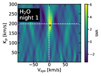
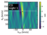
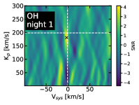
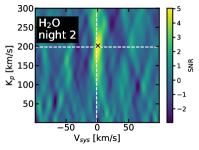
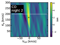
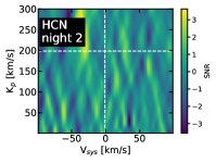
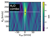
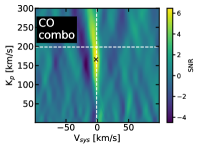
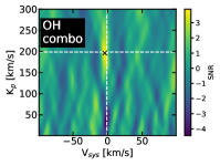
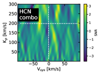
Figure 1: Cross-correlation signal-to-noise ratio (SNR) as a function of systemic velocity ($V_{sys}$) and planet Keplerian velocity ($K_{p}$) for detections of, from left to right, H₂O, CO, and OH on night 1 (top), night 2 (middle) and from both nights combined (bottom). SNR is calculated following Equation 1 after performing a $3\sigma$ clipping using astropy.stats.sigma_clipped_stats. For the CO detection, we used only the orders containing the two distinct absorption bands near 1.61 and 2.45 $\mu$m. Black x marks denote the maximum cross-correlation in each plot, while white dashed lines indicate expected values for WASP-76b from previous studies (West et al., 2016; Gaia Collaboration et al., 2018). All three molecules are clearly detected in both nights of data, and the combined data set shows SNRs of $6.93$, $6.47$, and $3.90$ for H₂O, CO, and OH, respectively. The right-most column shows non-detections of HCN on each night and in the combined data set.

In addition to detecting CO and OH in the atmosphere of WASP-76b, we found residual CO and OH trails at constant, near-zero systemic velocity. We attribute the CO to a residual signal from the host star WASP-76 and the OH to residual telluric airglow (Oliva et al., 2015). The two signals appear to overlap in velocity because of the relatively small barycentric velocity during both observations (6.12 km/s and 4.38 km/s on night 1 and 2, respectively). To keep these stellar and telluric signals from influencing the derived planetary CO and OH abundances, we applied a mask to the data which ignored contributions to the cross-correlation strength from exposures at orbital phases $-0.008<\phi<0.017$ where the planetary trail crosses the same velocities as the stellar and telluric trails (see Figure 2). The results we present here applied this mask evenly to all orders. However, we also tested applying this mask only to orders covering the strongest CO and OH features and found that the resulting elemental abundances, metallicity, and C/O ratio we derived for WASP-76b were within $1\sigma$ of the values retrieved from our main analysis.

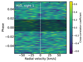
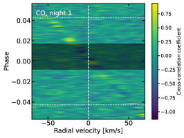
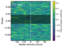
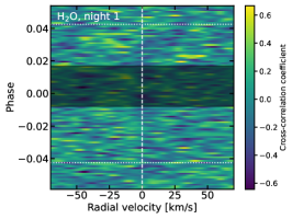
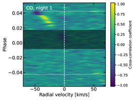
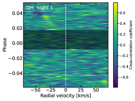
Figure 2: Trail plots showing cross-correlation strength as a function of radial velocity shift and orbital phase, in the rest frame of the planet WASP-76b, for H₂O (left), CO (middle), and OH (right) on night 1 (top) and night 2 (bottom). On all plots, horizontal white dotted lines indicate the beginning and end of transit and the vertical white dashed line indicates the location of the planetary signal. Signals in the trace that move diagonally from the upper left to lower right show the cross-correlation detections of the signal from the host star WASP-76 and tellurics. Grey shading indicates phases which were masked during the retrievals to remove any contamination from the stellar and telluric signals.

We also identified a feature on night 2 where the strength of the cross-correlation with the stellar and/or telluric signals suddenly became stronger and then switched to a strong anti-correlation at orbital phases of $\phi>0.02$ (see Figure 2). This feature is present in both the CO and OH trail plots. While the cause of this feature is unknown and outside the scope of this paper, it did not influence our conclusions because it showed no overlap with the planetary signal, as the planet’s line-of-sight velocity at those phases is large enough to Doppler shift its signal to the point where it is clearly separated from the stellar signal.

4 Retrieval Analysis

In order to investigate the impact of different retrieval frameworks on our inferred abundances, we performed two types of chemistry retrievals: a free chemistry retrieval (Section 4.1), and a self-consistent grid-based retrieval (Section 4.2). This choice is motivated by earlier work on WASP-18b (Brogi et al., 2023), where they found a different composition between free and self-consistent retrieval approaches. We additionally selected these two types of retrievals as representative end members of many possible types of retrievals, with one as free as possible and the other as self-consistent as possible.

4.1 Free Retrievals of Chemical Abundances

We first fit the data with retrievals based on the log-likelihood framework developed in Brogi & Line (2019), and using the model atmosphere framework described in Line et al. (2021). We used the up-to-date line lists for H₂O, CO, and OH mentioned in Section 3, as well as H₂-H₂ and H₂-He collision-induced absorption (Karman et al., 2019), and H^- bound-free and free-free absorption (Bell & Berrington, 1987; John, 1988).

We parameterized our one-dimensional atmosphere models with constant-with-altitude volume mixing ratios for the three detected gases and H^- bound-free and free-free opacity ($n_{H_{2}O}$, $n_{CO}$, $n_{OH}$, $n_{HmBF}$, $n_{HmFF}$), a three-parameter Guillot temperature-pressure (T-P) profile ($T_{0}$, $\gamma_{1}$, and $\kappa_{IR}$; Guillot, 2010), and a cloud-top pressure ($P_{c}$). We additionally fit for the planet Keplerian and system velocities ($K_{p}$ and $V_{sys}$), which affect the Doppler shift at which the planetary transmission signature is detected. Finally, we included as a nuisance parameter a scale factor on the reference planet radius ($\times R_{p}$). We initially fit for a phase offset to account for errors in the reported ephemeris, but we removed this from the final fits after initial retrievals showed it was consistent with zero. Our retrievals therefore contained a total of 12 free parameters.

Following Line et al. (2021), we convolved the model spectra with a kernel for instrumental broadening. We also applied a kernel for planetary rotation broadening during transit, following Equation 15 from Gandhi et al. (2022) and assuming a rotational velocity of 5.14 km/s. We multiplied the model (1-$(R_{p}/R_{*})^{2}$), appropriately Doppler shifted according to the Earth’s barycentric velocity and the planet’s $K_{p}$, $V_{sys}$, and orbital phase, by a matrix representing the eigenvectors discarded by the SVD detrending method we used to clean our data, creating a “model-injected” data cube. We then re-applied SVD detrending to this model injected data cube, cross-correlated the model with the SVD detrended data, and followed the methods of Brogi & Line (2019) to convert the cross-correlation strength to a log-likelihood. We then evaluated the log-likelihood within the context of the Python package pymultinest (Buchner et al., 2014a) to perform Bayesian inference and model selection. The only difference between our methods and those of Line et al. (2021) is that, as our observation is a transmission spectrum, our models are in units of transit depth, or the planet-to-star radius ratio squared (($R_{p}$/$R_{*}$)²).

Figure 3 shows the constraints derived from this retrieval. We retrieved abundances of $\log_{10}(n)=-4.66^{+1.34}_{-1.33}$, $-3.30^{+1.36}_{-1.30}$, and $-5.11^{+1.39}_{-1.33}$ for H₂O, CO, and OH, respectively. We converted these abundances into a total volatile metallicity ([(C+O)/H]) and carbon-to-oxygen ratio (C/O) relative to solar values using the equations

$$\left[\frac{\mathrm{C}+\mathrm{O}}{\mathrm{H}}\right]=\log_{10}\left(\frac{2n_{\mathrm{CO}}+n_{\mathrm{H}_{2}\mathrm{O}}+n_{\mathrm{OH}}}{2n_{\mathrm{H}_{2}}}\right)\\ -\log_{10}\left((\mathrm{C}/\mathrm{H})_{\odot}+(\mathrm{O}/\mathrm{H})_{\odot}\right),$$ (2)

and

$$\mathrm{C}/\mathrm{O}=\frac{n_{\mathrm{CO}}}{n_{\mathrm{H}_{2}\mathrm{O}}+n_{\mathrm{CO}}+n_{\mathrm{OH}}},$$ (3)

respectively. We used the solar C and O abundances as references because, while WASP-76 has a measured iron abundance of [Fe/H]$=0.23\pm 0.10$, it has no measured carbon or oxygen abundances (West et al., 2016). Additionally, prior research has shown that solar-type stars generally have near-solar C/O ratios (Fortney, 2012; Bedell et al., 2018). We refer throughout the rest of the paper to WASP-76b’s [Fe/H] when comparing metallicity values but to the solar C/O when comparing C/O ratios. We derived a volatile metallicity of $\left[\frac{\mathrm{C+O}}{\mathrm{H}}\right]=-0.14^{+1.36}_{-1.30}$ and a C/O ratio of $\mathrm{C/O}=0.94\pm 0.02$.

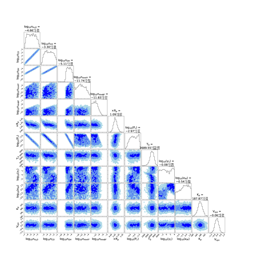
Figure 3: Posterior distributions for all parameters in the fiducial retrieval. Off-diagonal plots show 2D posterior probabilities for pairs of parameters, with 1, 2, and $3\sigma$ intervals shaded in dark, medium, and light blue. On-diagonal plots show marginalized posterior probability distributions for each parameter.

At face value, these results suggest that WASP-76b has a super-stellar metallicity but a significantly super-solar C/O ratio. However, at the high temperatures achieved in the upper atmosphere of WASP-76b, water dissociation is predicted to influence the retrieved oxygen abundance (e.g., Parmentier et al., 2018). Figure 4 compares our retrieved abundances to expectations from an equilibrium chemistry model for WASP-76b at a solar metallicity and C/O ratio. Above pressures of $\approx 10^{-2}$ bar, water is expected to dissociate into both OH molecules and atomic oxygen. Our data revealed the presence of both H₂O and OH, confirming that dissociation is influencing our observations. Additionally, a tentative detection of atomic O has been reported for WASP-76b in optical MAROON-X observations (Pelletier et al., 2023). IGRINS is not sensitive to atomic O, but at solar composition, chemical equilibrium models predict that $\lesssim 3$% of the oxygen would be in atomic form at the photosphere ($\approx 10^{-2}-10^{-3}$ bar), which will impact our estimates of the metallicity and C/O ratio by an amount much smaller than our retrieved error bars. The negligible influence of unaccounted atomic O differs significantly from the case of Brogi et al. (2023), which studied the higher-temperature, higher-gravity planet WASP-18b and found that $20-30$% of oxygen was in atomic form due to thermal dissociation, thus significantly influencing the estimated C/O ratio.

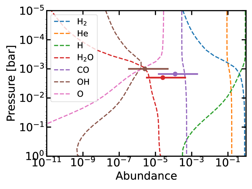
Figure 4: Comparison of retrieved abundances from the fiducial retrieval to expectations for a solar composition gas in chemical equilibrium. Dashed lines show expected abundance of various species as a function of pressure for a model with a composition consistent with the best-fit results from this retrieval ([M/H]$=-0.125$ and C/O$=0.9$). Solid points with $1\sigma$ error bars show retrieved abundances for H₂O (red), CO (purple), and OH (brown). The points are placed near the mean photospheric pressure across the observed wavelengths.

However, equilibrium chemistry models also indicate a large change in the abundance of water with pressure, due to the higher upper atmosphere temperatures driving dissociation of water, as seen in Figure 4. Our models which assume a constant abundance with pressure may therefore bias the retrieved abundance. To determine whether this bias shapes our retrieved volatile metallicity and C/O ratio, we ran a second set of retrievals where each molecular abundance profile was represented by two parameters: a deep atmosphere abundance ($n_{\mathrm{H}_{2}\mathrm{O}}$, $n_{\mathrm{CO}}$, and $n_{\mathrm{OH}}$) and a break pressure above which the abundance drops to zero ($P_{b,\mathrm{H}_{2}\mathrm{O}}$, $P_{b,\mathrm{CO}}$, and $P_{b,\mathrm{OH}}$).

Figures 5 and 6 shows the results of this pressure break-point retrieval. The retrieved deep atmosphere abundances of H₂O, CO, and OH are $\log_{10}(n)=-4.59^{+1.28}_{-0.92}$, $-3.91^{+1.26}_{-0.94}$, and $-5.59^{+1.31}_{-0.93}$, respectively. Based on these deep atmosphere abundances, the retrieved volatile metallicity and carbon-to-oxygen ratio are $\left[\frac{\mathrm{C}+\mathrm{O}}{\mathrm{H}}\right]=-0.70^{+1.27}_{-0.93}$ and C/O$=0.80^{+0.07}_{-0.11}$. The retrieved break pressures for CO and OH are consistent with the top of the atmosphere in the models, which indicates that the retrieval preferred a model where the CO and OH abundances are constant with altitude. However, the retrieved break pressure for H₂O is $\log_{10}P_{b,\mathrm{H}_{2}\mathrm{O}}=-3.28^{+0.94}_{-1.31}$. As shown in Figure 6, this is consistent with the expected pressure at which the water abundance would start to significantly decrease due to dissociation in an atmosphere in equilibrium and with approximately the same metallicity and C/O ratio as what was retrieved.

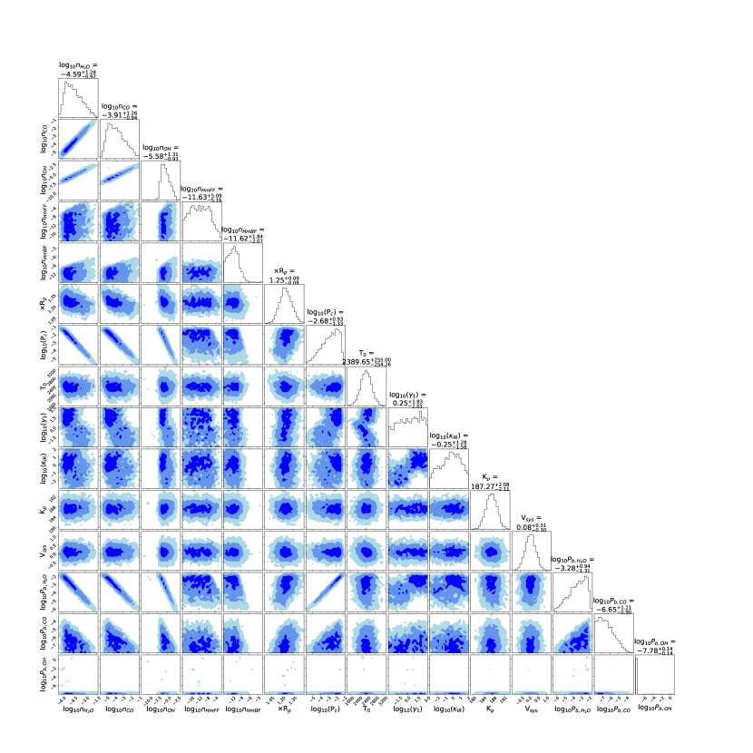
Figure 5: Same as Figure 3 but for the break pressure retrieval. In this retrieval, each detected molecule is represented with two parameters: a deep atmosphere abundance ($\log_{10}(n)$) and a break pressure where the abundance drops to zero ($P_{b}$).

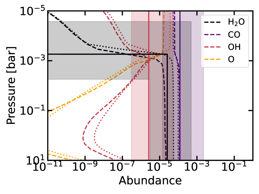
Figure 6: Comparison of retrieved abundances from the break pressure retrieval to expectations for models in chemical equilibrium. Solid lines with $1\sigma$ shaded error bars show retrieved profiles for H₂O (black), CO (purple), and OH (red). As described in Section 4.1, each abundance was fit with a two-parameter model including a deep atmosphere abundance and a pressure at which the abundance dropped to 0. For CO and OH, the retrieved break pressure was consistent with the top of the atmosphere, indicating the retrieval preferred a model with constant abundances with altitude for both gases. Dashed and dotted lines show predictions from chemical equilibrium models with compositions consistent with the best-fit results from this retrieval ([M/H]$=-0.75$ and C/O$=0.8$) and from the self-consistent gridtrieval ([M/H]$=-0.75$ and C/O$=0.6$), respectively.

We also investigated performing retrievals separately on the first and second half of the transits, to search for inhomogeneities between the two limbs. However, our data were not high enough signal-to-noise to constrain any limb asymmetries.

4.2 Self-Consistent Gridtrievals

In addition to the free chemistry retrievals listed above, we ran a self-consistent “gridtrieval” for WASP-76b using the grid-based retrieval framework described in Brogi et al. (2023). The gridtrieval framework fits the data by interpolating between pre-computed models which self-consistently calculate the T-P profile and molecular chemistry based on provided elemental abundances. We used a framework identical to that described in Brogi et al. (2023) to calculate the grid of self-consistent models for WASP-76b. The gridtrieval parameterizes the atmospheric composition and temperature with three parameters: a heat redistribution efficiency parameter ($f$), an atmospheric metallicity ([M/H]) which scaled all elements (re-normalizing to H), and a carbon-to-oxygen ratio (C/O) (adjusted while preserving the sum of C+O after the [M/H] scaling). In addition to these three parameters, we also fit for a radius scale factor ($\times R_{p}$), cloud-top pressure ($P_{c}$), and velocities ($K_{p}$ and $V_{sys}$) as described above, for a total of seven free parameters. A pairs plot for the gridtrieval is shown in Figure 7.

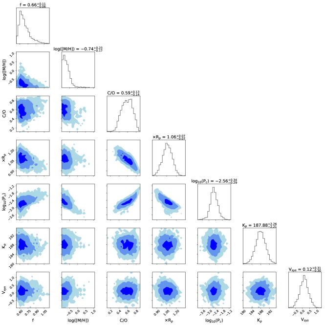
Figure 7: Same as for Figure 3, but for the gridtrieval described in Section 4.2.

The gridtrieval retrieved a metallicity of [M/H]$=-0.74^{+0.23}_{-0.17}$ and a carbon-to-oxygen ratio of C/O$=0.59^{+0.13}_{-0.14}$. The expected atmospheric composition for a planet in chemical equilirium with this metallicity and C/O ratio are also shown in Figure 6. These values are consistent to within $1\sigma$ with the result derived from the break pressure retrieval. We note that grid-based retrievals tend to produce tighter constraints than more flexible free retrievals owing to the assumption of 1D radiative-convective-thermochemical equilibrium which rules out various abundance/temperature combinations that don’t fall within those self-consistent assumptions (e.g., Brogi et al., 2023).

5 Retrievals of Velocity Offsets

Previous observations of WASP-76b at optical wavelengths have shown the “Ehrenreich effect”, or an asymmetry in the velocity at which iron (Ehrenreich et al., 2020) and other atomic species (Pelletier et al., 2023) were detected as a function of phase. This asymmetry has been suggested to be due to differences in Fe abundance (Ehrenreich et al., 2020), temperature-pressure (T-P) profiles (Wardenier et al., 2021; Pelletier et al., 2023), cloud opacity (Savel et al., 2022; Pelletier et al., 2023), and/or wind speeds (Gandhi et al., 2022) between the eastern and western limbs. As shown in Figure 2, our trail plots do not show high enough signals to detect deviations in radial velocity for H₂O, CO, or OH as a function of orbital phase as was found for iron. However, Figure 1 shows that on both nights we see differences in the overall $V_{sys}$ and $K_{p}$ at which each of these three species are detected. In order to investigate the significance of these velocity differences, we performed another set of atmospheric retrievals where the only free parameters were $V_{sys}$, $K_{p}$, and $\times R_{p}$. We did one retrieval each for the three gases whose abundances we constrain, and we fixed the abundance profile of the gas to the best-fit values from the break pressure retrieval. Table 1 lists the offsets between the retrieved velocities and the values expected from previous radial velocity observations of WASP-76b’s orbit ($K_{p}=196.52\pm 0.94$ km/s and $V_{sys}=-1.11\pm 0.50$ km/s, Ehrenreich et al., 2020; Gaia Collaboration et al., 2018). We compared these velocity offsets to those predicted from 3D general circulation models of WASP-76b (Wardenier et al., 2023) to interpret them in terms of the expected circulation patterns in the planet’s atmosphere.

Gas	$\Delta K_{p}$ [km/s]	$\Delta V_{sys}$ [km/s]
H2O	$-1.1^{+3.0}_{-2.9}$	$2.42^{+0.39}_{-0.38}$
CO	$-18.8\pm 2.7$	$0.69\pm 0.38$
OH	$3.2^{+5.5}_{-5.2}$	$-2.97^{+0.70}_{-0.75}$

Table 1: Retrieved systemic velocity ($V_{sys}$) and Keplerian velocity ($K_{p}$) offsets from expected values (West et al., 2016; Gaia Collaboration et al., 2018) for retrievals where only velocity offsets and a scale factor were allowed to vary.

Wardenier et al. (2023) divide atmospheric species into those whose signal primarily comes from the dayside or nightside of the planet. H₂O is classified as a nightside species, as dissociation on the dayside reduces the H₂O abundance in that hemisphere. Conversely, dayside dissociation increases the OH abundance, so OH is classified as a dayside species. Finally, while CO is expected to be present across the entire planet in similar abundances (Savel et al., 2023), the hotter temperature on the dayside means that the majority of the CO absorption originates from the dayside, making it a dayside species.

In their 3D models, dayside species exhibit a negative shift in both $V_{sys}$, because planetary winds overall blueshift the absorption features, and $K_{p}$, because in 3D models the signals become more blueshifted throughout the course of the transit (Wardenier et al., 2023). While our data are not precise enough to resolve an increasing blueshift in the trail plots shown in Figure 2, we do find a negative $K_{p}$ shift for CO of $\Delta K_{p}=-18.8$ km/s. This is consistent with the findings of Wardenier et al. (2023), who found a $\Delta K_{p}\approx 20$ km/s for CO in most of their models. For OH, we do not see a similar shift in $K_{p}$, as predicted by Wardenier et al. (2023). However, the relative offset in $V_{sys}$ between CO and OH is similar to what is found by Wardenier et al. (2023) - their models predict OH to have a $V_{sys}$ about $0.5-1$ km/s less than that of CO, while we find OH to have a $V_{sys}$ 3.6 km/s less than CO.

For the nightside species H₂O, our slight $K_{p}$ offset of $-1.1$ km/s is consistent with the results of Wardenier et al. (2023), which predict a smaller offset of about $5-10$ km/s for nightside species. However, the redshifted $V_{sys}$ we see for H₂O cannot be explained by any of their models. In theory, H₂O could have a redshifted $V_{sys}$ on a windless planet if it was present on the colder leading limb but dissociated on the warmer trailing limb, because in this scenario the H₂O detection would come entirely from a region of the planet rotating away from the observer (Wardenier et al., 2023). However, our data are not precise enough to detect phase-resolved differences in abundances, so we cannot confirm whether H₂O is indeed only present on the leading limb. In addition, when realistic wind speeds are added to the planet, none of the models of Wardenier et al. (2023) show a net redshifted $V_{sys}$ for H₂O. However, models incorporating magnetic drag do retrieve similar velocity differences as what we see between H₂O and CO, even if the absolute values are not as redshifted (Beltz et al., 2023). More precise phase-resolved data or models incorporating more effects such as different magnetic drag parameterizations (Beltz et al., 2023) will be required to fully understand our detection of redshifted $V_{sys}$ for H₂O.

6 Discussion

6.1 Comparison to Previous Carbon and Oxygen Detections

Several of the species we detected have been previously measured in transmission spectra of WASP-76b. H₂O has been previously detected using HST (Edwards et al., 2020; Fu et al., 2021). The two published HST retrievals disagree on the overall abundance of water - Edwards et al. (2020) reported a retrieved H₂O abundance of $\log_{10}(n_{\mathrm{H}_{2}\mathrm{O}})=-2.85^{+0.42}_{-0.71}$, while Fu et al. (2021) found an oxygen abundance of $\log_{10}(n_{\mathrm{O}})=-4.34^{+0.43}_{-0.48}$. In the break pressure model, we found an overall oxygen abundance of $\log_{10}(n_{\mathrm{O}})=\log_{10}(n_{\mathrm{H}_{2}\mathrm{O}}+n_{\mathrm{OH}}+n_{\mathrm{CO}})=-3.82^{+1.05}_{-0.78}$, which is consistent with the results of both Edwards et al. (2020) and Fu et al. (2021).

Dayside observations of WASP-76b both at high-resolution with CRIRES+ (Yan et al., 2023) and at low-resolution with Spitzer also showed detections of CO in its atmosphere. Yan et al. (2023) found a CO abundance of $\log_{10}(n_{CO})=-3.6^{+1.8}_{-1.6}$, and Fu et al. (2021) report an overall carbon abundance of $\log_{10}(n_{C})=-4.42^{+0.48}_{-0.66}$. Our retrieved CO abundance is also consistent with both of these results within $1\sigma$.

Previous high-resolution transit observations of WASP-76b have reported results in disagreement with each other. Sánchez-López et al. (2022) observed WASP-76b with CARMENES and reported a similar detection of H₂O, but at a significantly higher $K_{p}=249\pm 38$ and lower $V_{sys}=-14.3\pm 2.6$. They additionally reported a detection of HCN. On the other hand, (Hood et al., 2024) observed WASP-76b with SPIRou and detected H₂O and CO but not HCN or OH. They reported best-fit abundances of $\log_{10}(n_{\mathrm{H}_{2}\mathrm{O}})=-4.52\pm 0.77$ and $\log_{10}(n_{\mathrm{CO}})=-3.09\pm 1.05$, with upper limits of $\log_{10}(n_{\mathrm{OH}})<-6$ and $\log_{10}(n_{\mathrm{HCN}})<-5.5$ and a resulting retrieved C/O ratio of $0.94\pm 0.39$.

To compare our results to these previous high-resolution transit observations, we performed an additional retrieval where we added HCN as a free parameter. We found an unconstrained abundance with a $2\sigma$ upper limit of $\log(\mathrm{HCN})=-4.95$. Our results are thus in good agreement with those of Hood et al. (2024). Our retrieved OH abundance and upper limit on the HCN abundance are consistent with their derived upper limits. Additionally, our H₂O and CO abundances and C/O ratio are within their $1\sigma$ errors. However, our results disagree with those of Sánchez-López et al. (2022), both in our inability to detect HCN and in the different velocity shifts we retrieve for H₂O. We hypothesize that this may be due to a difference in data reduction methods. Both our reduction and that of Hood et al. (2024) used similar applications of principal component analysis/SVD, with the same number of components removed from all orders and across all molecules being analyzed. However, Sánchez-López et al. (2022) removed different numbers of components in order to optimize detections of each molecule individually. This may have resulted in a sporadic detection of HCN through over-optimization of the data reduction.

6.2 Potential Formation Scenarios for WASP-76b and Exoplanet C/O Ratios in General

Our results indicate that the atmosphere of WASP-76b has either a stellar metallicity and a super-solar C/O ratio (from the break pressure free retrieval) or a sub-stellar metallicity and a solar C/O ratio (from the gridtrieval). Previous research has suggested that a C/O ratio near consistent with solar and stellar or sub-stellar metallicities could be consistent with many origin locations within the disk, depending on factors such as the relative rate of solid and gas accretion (e.g., Madhusudhan et al., 2014; Khorshid et al., 2022). On the other hand, a super-solar C/O ratio could result from gas-dominated accretion beyond the CO snowline in the protoplanetary disk and subsequent migration (e.g., Madhusudhan et al., 2014; Öberg & Bergin, 2016; Madhusudhan et al., 2017) or in situ formation between the soot line and water snow line (Chachan et al., 2023). These two scenarios of formation could be distinguished by the refractory element enrichment, as formation outside the CO snow line is predicted to show refractory enrichments $\lesssim 1\times$ solar, while formation between the soot line and water snow line is expected to have higher refractory abundances of $\gtrsim 10\times$ solar (Chachan et al., 2023).

Pelletier et al. (2023) and Gandhi et al. (2023) recently reported the abundances of the refractory elements Fe, Mg, Cr, Mn, Ni, V, Ba, and Ca on WASP-76b, which ranged from 0.14 to 18.20$\times$ solar. The intermediate values of these refractory abundances, with most between $1-10\times$ solar, make it difficult to distinguish between the two proposed formation scenarios. However, future work to measure abundances of other elements such as nitrogen (Öberg & Bergin, 2016; Ohno & Fortney, 2023) and sulfur (Polman et al., 2023) may provide more paths to understand the formation of WASP-76b.

While the C/O ratio of WASP-76b alone is inconclusive in determining its formation, the launch of JWST in 2021 and the advent of methods for retrieving abundances from high-resolution spectroscopy are for the first time allowing intercomparison of a sample of exoplanets with C/O ratios constrained from observation of both carbon- and oxygen-bearing species. Figure 8 and Table 2 shows the full sample of planets with constrained C/O ratios. While there are a wide variety of reported values, most are weighted toward super-solar C/O ratios. After calculating a single averaged value for each planet for which there are multiple reported values from different sources, the full sample has a weighted mean C/O ratio of 0.89 and a median of 0.72.

There is already significant scatter in the reported C/O values, indicating that there may be a variety of formation mechanisms at play. The sample of planets with well-constrained C/O ratios is also still relatively small, so future work to measure C/O ratios on a wider population of planets may further elucidate any population-level trends.

Planet Name	C/O Ratio	Provenance	Reference
HD 149026b	$0.84\pm 0.03$	JWST (NIRCam)	Bean et al. (2023)
	$0.67^{+0.06}_{-0.27}$		Gagnebin et al. (2024)
HD 209458b	$0.99^{+0.01}_{-0.02}$	High-res (CRIRES)	Gandhi et al. (2019)
HIP 65Ab	$0.71^{+0.16}_{-0.47}$	High-res (IGRINS)	Bazinet et al. (2024)
MASCARA-1b	$0.68^{+0.12}_{-0.22}$	High-res (CRIRES+)	Ramkumar et al. (2023)
WASP-43b	$0.78\pm 0.09$	High-res (CRIRES+)	Lesjak et al. (2023)
WASP-76b	$0.80^{+0.07}_{-0.11}$	High-res (IGRINS)	This work
	$0.59^{+0.13}_{-0.14}$
	$0.94\pm 0.39$	High-res (SPIRou)	Hood et al. (2024)
WASP-77Ab	$0.59\pm 0.08$	High-res (IGRINS)	Line et al. (2021)
	$0.36^{+0.10}_{-0.09}$	JWST (NIRSpec)	August et al. (2023)
	$0.57\pm 0.06$	JWST/NIRSpec + IGRINS combined	Smith et al. (2024)
	$0.54\pm 0.12$	JWST/NIRSpec + HST/WFC3 combined	Edwards & Changeat (2024)
WASP-127b	$0.56^{+0.05}_{-0.07}$	High-res (CRIRES+)	Nortmann et al. (2024)
Jupiter	$0.90^{+1.54}_{-0.35}$	C from Galileo, O from Juno	Wong et al. (2004); Li et al. (2024)

Table 2: List of planets with well-constrained C/O ratios, measured through direct observation of both carbon- and oxygen-bearing species. Note that results which only reported upper or lower limits (e.g., Brogi et al., 2023; Bell et al., 2023) are not included here.

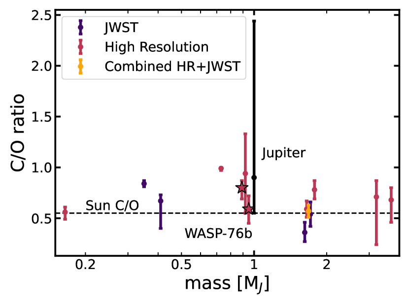
Figure 8: Carbon-to-oxygen (C/O) ratio as a function of mass for all planets with constrained abundances of both oxygen-bearing and carbon-bearing species. Purple, pink, and yellow points indicate results from JWST, high-resolution observations, and combined analyses of both JWST and high-resolution data (citations given in Table 2). The black point indicates the value for Jupiter based on the Galileo and Juno missions. The pink points with black outlined, star-shaped markers are our results for WASP-76b. Planets with multiple measurements have small offsets in mass applied between the different results for clarity. While there is no clear trend with mass, overall the population of exoplanets shows a mean C/O ratio greater than solar.

7 Conclusions

We present observations of the ultra-hot Jupiter WASP-76b with Gemini-S/IGRINS between $1.4-2.4$ $\mu$m, reduced with the IGRINS PLP (Sim et al., 2014; Lee & Gullikson, 2016) and analyzed with the newly developed IGRINS_transit custom pipeline for IGRINS transiting exoplanet data analysis. We detected the presence of H₂O, CO, and OH in the atmosphere of WASP-76b.

We performed three sets of retrievals to determine the abundances of these species. First, we retrieved constant-with-altitude abundances for each species and found a volatile metallicity consistent with the stellar metallicity but a significantly super-solar C/O ratio. However, water dissociation in the upper atmospheres of ultra-hot Jupiters is expected to bias retrieved constant-with-altitude abundances (e.g., Parmentier et al., 2018). We therefore performed a second set of retrievals which included a break pressure parameterization above which abundances dropped to zero to estimate the effect of dissociation in the upper atmosphere. We found that this second retrieval resulted in a stellar metallicity and super-solar C/O ratio ($\left[\frac{\mathrm{C}+\mathrm{O}}{\mathrm{H}}\right]=-0.70^{+1.27}_{-0.93}$ and C/O$=0.80^{+0.07}_{-0.11}$). We also retrieved a water break pressure of $\log_{10}P_{b,\mathrm{H}_{2}\mathrm{O}}=-3.28^{+0.94}_{-1.31}$, which as shown in Figure 6 is consistent with expectations for the pressure at which the water abundance begins to decrease sharply in a model with the same approximate composition as what we retrieve for WASP-76b. Finally, we performed a gridtrieval using a set of pre-computed self-consistent thermochemical equilibrium models, which slightly favored a sub-stellar metallicity and solar C/O ratio ($\left[\frac{\mathrm{C}+\mathrm{O}}{\mathrm{H}}\right]=-0.74^{+0.23}_{-0.17}$ and C/O$=0.59^{+0.13}_{-0.14}$), but was consistent within $1\sigma$ with the results of the break pressure retrieval.

Our derived metallicity and C/O ratio are consistent with a wide variety of formation pathways for WASP-76b (e.g., Madhusudhan et al., 2014; Khorshid et al., 2022). When placed in the broader context of all exoplanets with C/O ratios based on simultaneous measurements of carbon- and oxygen-bearing species, the population as a whole seems skewed toward super-solar C/O ratios. Such super-solar C/O ratios could result from accretion beyond the CO snowline (e.g., Madhusudhan et al., 2014; Öberg & Bergin, 2016; Madhusudhan et al., 2017) or in-situ formation between the soot line and water snow line (Chachan et al., 2023). However, there is significant scatter among the relatively small population of exoplanets with constrained C/O ratios. Trends in the planetary population may become clearer as JWST and high-resolution ground-based observations measure precise C/O ratios for a larger sample of planets. Additionally, future observations of WASP-76b with JWST would serve to confirm its composition.

In addition to measuring the composition of WASP-76b, we compared the velocities at which H₂O, CO, and OH were detected to 3D GCM predictions (Wardenier et al., 2023). We found that the velocity offsets observed for CO and OH were relatively consistent with model expectations. However, the H₂O detection showed a redshifted systemic velocity, which cannot be matched by any of the 3D models of Wardenier et al. (2023). Future, more precise observations which can resolve the two limbs of the transiting planet separately, or additional models taking into account effects such as magnetic drag (Beltz et al., 2023) may help to understand this H₂O velocity offset.

References

- Astropy Collaboration et al. (2013) Astropy Collaboration, Robitaille, T. P., Tollerud, E. J., et al. 2013, A&A, 558, A33, doi: 10.1051/0004-6361/201322068
- Astropy Collaboration et al. (2018) Astropy Collaboration, Price-Whelan, A. M., Sipőcz, B. M., et al. 2018, AJ, 156, 123, doi: 10.3847/1538-3881/aabc4f
- Astropy Collaboration et al. (2022) Astropy Collaboration, Price-Whelan, A. M., Lim, P. L., et al. 2022, ApJ, 935, 167, doi: 10.3847/1538-4357/ac7c74
- August et al. (2023) August, P. C., Bean, J. L., Zhang, M., et al. 2023, ApJ, 953, L24, doi: 10.3847/2041-8213/ace828
- Azevedo Silva et al. (2022) Azevedo Silva, T., Demangeon, O. D. S., Santos, N. C., et al. 2022, A&A, 666, L10, doi: 10.1051/0004-6361/202244489
- Bazinet et al. (2024) Bazinet, L., Pelletier, S., Benneke, B., Salinas, R., & Mace, G. N. 2024, AJ, 167, 206, doi: 10.3847/1538-3881/ad3071
- Bean et al. (2023) Bean, J. L., Xue, Q., August, P. C., et al. 2023, Nature, 618, 43, doi: 10.1038/s41586-023-05984-y
- Bedell et al. (2018) Bedell, M., Bean, J. L., Meléndez, J., et al. 2018, ApJ, 865, 68, doi: 10.3847/1538-4357/aad908
- Bell & Berrington (1987) Bell, K. L., & Berrington, K. A. 1987, Journal of Physics B: Atomic & Molecular Physics, 20, 1
- Bell et al. (2023) Bell, T. J., Welbanks, L., Schlawin, E., et al. 2023, Nature, 623, 709, doi: 10.1038/s41586-023-06687-0
- Beltz et al. (2023) Beltz, H., Rauscher, E., Kempton, E. M. R., Malsky, I., & Savel, A. B. 2023, AJ, 165, 257, doi: 10.3847/1538-3881/acd24d
- Brogi & Line (2019) Brogi, M., & Line, M. R. 2019, AJ, 157, 114, doi: 10.3847/1538-3881/aaffd3
- Brogi et al. (2023) Brogi, M., Emeka-Okafor, V., Line, M. R., et al. 2023, AJ, 165, 91, doi: 10.3847/1538-3881/acaf5c
- Buchner et al. (2014a) Buchner, J., Georgakakis, A., Nandra, K., et al. 2014a, A&A, 564, A125, doi: 10.1051/0004-6361/201322971
- Buchner et al. (2014b) —. 2014b, A&A, 564, A125, doi: 10.1051/0004-6361/201322971
- Casasayas-Barris et al. (2021) Casasayas-Barris, N., Orell-Miquel, J., Stangret, M., et al. 2021, A&A, 654, A163, doi: 10.1051/0004-6361/202141669
- Chachan et al. (2023) Chachan, Y., Knutson, H. A., Lothringer, J., & Blake, G. A. 2023, ApJ, 943, 112, doi: 10.3847/1538-4357/aca614
- de Kok et al. (2013) de Kok, R. J., Brogi, M., Snellen, I. A. G., et al. 2013, A&A, 554, A82, doi: 10.1051/0004-6361/201321381
- Deibert et al. (2021) Deibert, E. K., de Mooij, E. J. W., Jayawardhana, R., et al. 2021, ApJ, 919, L15, doi: 10.3847/2041-8213/ac2513
- Deibert et al. (2023) —. 2023, AJ, 166, 141, doi: 10.3847/1538-3881/acebdc
- Edwards & Changeat (2024) Edwards, B., & Changeat, Q. 2024, ApJ, 962, L30, doi: 10.3847/2041-8213/ad2000
- Edwards et al. (2020) Edwards, B., Changeat, Q., Baeyens, R., et al. 2020, AJ, 160, 8, doi: 10.3847/1538-3881/ab9225
- Ehrenreich et al. (2020) Ehrenreich, D., Lovis, C., Allart, R., et al. 2020, Nature, 580, 597, doi: 10.1038/s41586-020-2107-1
- Fortney (2012) Fortney, J. J. 2012, ApJ, 747, L27, doi: 10.1088/2041-8205/747/2/L27
- Fu et al. (2021) Fu, G., Deming, D., Lothringer, J., et al. 2021, AJ, 162, 108, doi: 10.3847/1538-3881/ac1200
- Gagnebin et al. (2024) Gagnebin, A., Mukherjee, S., Fortney, J. J., & Batalha, N. E. 2024, arXiv e-prints, arXiv:2404.17658, doi: 10.48550/arXiv.2404.17658
- Gaia Collaboration et al. (2018) Gaia Collaboration, Brown, A. G. A., Vallenari, A., et al. 2018, A&A, 616, A1, doi: 10.1051/0004-6361/201833051
- Gandhi et al. (2022) Gandhi, S., Kesseli, A., Snellen, I., et al. 2022, MNRAS, 515, 749, doi: 10.1093/mnras/stac1744
- Gandhi et al. (2019) Gandhi, S., Madhusudhan, N., Hawker, G., & Piette, A. 2019, AJ, 158, 228, doi: 10.3847/1538-3881/ab4efc
- Gandhi et al. (2023) Gandhi, S., Kesseli, A., Zhang, Y., et al. 2023, AJ, 165, 242, doi: 10.3847/1538-3881/accd65
- Gharib-Nezhad et al. (2021) Gharib-Nezhad, E., Iyer, A. R., Line, M. R., et al. 2021, ApJS, 254, 34, doi: 10.3847/1538-4365/abf504
- Giacobbe et al. (2021) Giacobbe, P., Brogi, M., Gandhi, S., et al. 2021, Nature, 592, 205, doi: 10.1038/s41586-021-03381-x
- Gordon et al. (2022) Gordon, I., Rothman, L., Hargreaves, R., et al. 2022, Journal of Quantitative Spectroscopy and Radiative Transfer, 277, 107949, doi: https://doi.org/10.1016/j.jqsrt.2021.107949
- Guillot (2010) Guillot, T. 2010, A&A, 520, A27, doi: 10.1051/0004-6361/200913396
- Harris et al. (2020) Harris, C. R., Millman, K. J., van der Walt, S. J., et al. 2020, Nature, 585, 357, doi: 10.1038/s41586-020-2649-2
- Hood et al. (2024) Hood, T., Debras, F., Moutou, C., et al. 2024, arXiv e-prints, arXiv:2403.19434, doi: 10.48550/arXiv.2403.19434
- Hunter (2007) Hunter, J. D. 2007, Computing in Science & Engineering, 9, 90, doi: 10.1109/MCSE.2007.55
- John (1988) John, T. L. 1988, A&A, 193, 189
- Karman et al. (2019) Karman, T., Gordon, I. E., van der Avoird, A., et al. 2019, Icarus, 328, 160, doi: 10.1016/j.icarus.2019.02.034
- Kawauchi et al. (2022) Kawauchi, K., Narita, N., Sato, B., & Kawashima, Y. 2022, PASJ, 74, 225, doi: 10.1093/pasj/psab120
- Kesseli & Snellen (2021) Kesseli, A. Y., & Snellen, I. A. G. 2021, ApJ, 908, L17, doi: 10.3847/2041-8213/abe047
- Kesseli et al. (2022) Kesseli, A. Y., Snellen, I. A. G., Casasayas-Barris, N., Mollière, P., & Sánchez-López, A. 2022, AJ, 163, 107, doi: 10.3847/1538-3881/ac4336
- Khorshid et al. (2022) Khorshid, N., Min, M., Désert, J. M., Woitke, P., & Dominik, C. 2022, A&A, 667, A147, doi: 10.1051/0004-6361/202141455
- Landman et al. (2021) Landman, R., Sánchez-López, A., Mollière, P., et al. 2021, A&A, 656, A119, doi: 10.1051/0004-6361/202141696
- Lee & Gullikson (2016) Lee, J.-J., & Gullikson, K. 2016, Plp: V2.1 Alpha 3, v2.1-alpha.3, Zenodo, Zenodo, doi: 10.5281/zenodo.56067
- Lesjak et al. (2023) Lesjak, F., Nortmann, L., Yan, F., et al. 2023, A&A, 678, A23, doi: 10.1051/0004-6361/202347151
- Li et al. (2024) Li, C., Allison, M., Atreya, S., et al. 2024, Icarus, 414, 116028, doi: 10.1016/j.icarus.2024.116028
- Li et al. (2015) Li, G., Gordon, I. E., Rothman, L. S., et al. 2015, ApJS, 216, 15, doi: 10.1088/0067-0049/216/1/15
- Line et al. (2021) Line, M. R., Brogi, M., Bean, J. L., et al. 2021, Nature, 598, 580, doi: 10.1038/s41586-021-03912-6
- Lothringer et al. (2021) Lothringer, J. D., Rustamkulov, Z., Sing, D. K., et al. 2021, ApJ, 914, 12, doi: 10.3847/1538-4357/abf8a9
- Madhusudhan et al. (2014) Madhusudhan, N., Amin, M. A., & Kennedy, G. M. 2014, ApJ, 794, L12, doi: 10.1088/2041-8205/794/1/L12
- Madhusudhan et al. (2017) Madhusudhan, N., Bitsch, B., Johansen, A., & Eriksson, L. 2017, MNRAS, 469, 4102, doi: 10.1093/mnras/stx1139
- Mansfield et al. (2021) Mansfield, M., Line, M. R., Bean, J. L., et al. 2021, Nature Astronomy, 5, 1224, doi: 10.1038/s41550-021-01455-4
- May et al. (2021) May, E. M., Komacek, T. D., Stevenson, K. B., et al. 2021, AJ, 162, 158, doi: 10.3847/1538-3881/ac0e30
- Mollière et al. (2022) Mollière, P., Molyarova, T., Bitsch, B., et al. 2022, ApJ, 934, 74, doi: 10.3847/1538-4357/ac6a56
- Mordasini et al. (2016) Mordasini, C., van Boekel, R., Mollière, P., Henning, T., & Benneke, B. 2016, ApJ, 832, 41, doi: 10.3847/0004-637X/832/1/41
- Nortmann et al. (2024) Nortmann, L., Lesjak, F., Yan, F., et al. 2024, arXiv e-prints, arXiv:2404.12363, doi: 10.48550/arXiv.2404.12363
- Öberg & Bergin (2016) Öberg, K. I., & Bergin, E. A. 2016, ApJ, 831, L19, doi: 10.3847/2041-8205/831/2/L19
- Öberg et al. (2011) Öberg, K. I., Murray-Clay, R., & Bergin, E. A. 2011, ApJ, 743, L16, doi: 10.1088/2041-8205/743/1/L16
- Ohno & Fortney (2023) Ohno, K., & Fortney, J. J. 2023, ApJ, 946, 18, doi: 10.3847/1538-4357/acafed
- Oliva et al. (2015) Oliva, E., Origlia, L., Scuderi, S., et al. 2015, A&A, 581, A47, doi: 10.1051/0004-6361/201526291
- Parmentier et al. (2018) Parmentier, V., Line, M. R., Bean, J. L., et al. 2018, A&A, 617, A110, doi: 10.1051/0004-6361/201833059
- Pelletier et al. (2021) Pelletier, S., Benneke, B., Darveau-Bernier, A., et al. 2021, AJ, 162, 73, doi: 10.3847/1538-3881/ac0428
- Pelletier et al. (2023) Pelletier, S., Benneke, B., Ali-Dib, M., et al. 2023, arXiv e-prints, arXiv:2306.08739, doi: 10.48550/arXiv.2306.08739
- Polman et al. (2023) Polman, J., Waters, L. B. F. M., Min, M., Miguel, Y., & Khorshid, N. 2023, A&A, 670, A161, doi: 10.1051/0004-6361/202244647
- Polyansky et al. (2018) Polyansky, O. L., Kyuberis, A. A., Zobov, N. F., et al. 2018, MNRAS, 480, 2597, doi: 10.1093/mnras/sty1877
- Ramkumar et al. (2023) Ramkumar, S., Gibson, N. P., Nugroho, S. K., Maguire, C., & Fortune, M. 2023, MNRAS, 525, 2985, doi: 10.1093/mnras/stad2476
- Sánchez-López et al. (2022) Sánchez-López, A., Landman, R., Mollière, P., et al. 2022, A&A, 661, A78, doi: 10.1051/0004-6361/202142591
- Savel et al. (2023) Savel, A. B., Kempton, E. M. R., Rauscher, E., et al. 2023, ApJ, 944, 99, doi: 10.3847/1538-4357/acb141
- Savel et al. (2022) Savel, A. B., Kempton, E. M. R., Malik, M., et al. 2022, ApJ, 926, 85, doi: 10.3847/1538-4357/ac423f
- Schneider & Bitsch (2021a) Schneider, A. D., & Bitsch, B. 2021a, A&A, 654, A71, doi: 10.1051/0004-6361/202039640
- Schneider & Bitsch (2021b) —. 2021b, A&A, 654, A72, doi: 10.1051/0004-6361/202141096
- Seidel et al. (2019) Seidel, J. V., Ehrenreich, D., Wyttenbach, A., et al. 2019, A&A, 623, A166, doi: 10.1051/0004-6361/201834776
- Sim et al. (2014) Sim, C. K., Le, H. A. N., Pak, S., et al. 2014, Advances in Space Research, 53, 1647, doi: 10.1016/j.asr.2014.02.024
- Smith et al. (2024) Smith, P. C. B., Line, M. R., Bean, J. L., et al. 2024, AJ, 167, 110, doi: 10.3847/1538-3881/ad17bf
- Tabernero et al. (2021) Tabernero, H. M., Zapatero Osorio, M. R., Allart, R., et al. 2021, A&A, 646, A158, doi: 10.1051/0004-6361/202039511
- Virtanen et al. (2021) Virtanen, P., Gommers, R., Burovski, E., et al. 2021, scipy/scipy: SciPy 1.6.3, v1.6.3, Zenodo, Zenodo, doi: 10.5281/zenodo.4718897
- von Essen et al. (2020) von Essen, C., Mallonn, M., Hermansen, S., et al. 2020, A&A, 637, A76, doi: 10.1051/0004-6361/201937169
- Wardenier et al. (2021) Wardenier, J. P., Parmentier, V., Lee, E. K. H., Line, M. R., & Gharib-Nezhad, E. 2021, MNRAS, 506, 1258, doi: 10.1093/mnras/stab1797
- Wardenier et al. (2023) Wardenier, J. P., Parmentier, V., Line, M. R., & Lee, E. K. H. 2023, arXiv e-prints, arXiv:2307.04931, doi: 10.48550/arXiv.2307.04931
- Weiner Mansfield & Line (2024) Weiner Mansfield, M., & Line, M. R. 2024, IGRINS_transit: analyze exoplanet transit observations taken with Gemini-S/IGRINS, 1.0, Zenodo, doi: 10.5281/zenodo.11106414
- West et al. (2016) West, R. G., Hellier, C., Almenara, J. M., et al. 2016, A&A, 585, A126, doi: 10.1051/0004-6361/201527276
- Wong et al. (2004) Wong, M. H., Mahaffy, P. R., Atreya, S. K., Niemann, H. B., & Owen, T. C. 2004, Icarus, 171, 153, doi: 10.1016/j.icarus.2004.04.010
- Yan et al. (2023) Yan, F., Nortmann, L., Reiners, A., et al. 2023, A&A, 672, A107, doi: 10.1051/0004-6361/202245371