Compact quantum algorithms that can potentially maintain quantum advantage for solving time-dependent differential equations

Abstract

Many claims of computational advantages have been made for quantum computing over classical, but they have not been demonstrated for practical problems. Here, we present algorithms for solving time-dependent PDEs governing fluid flow problems. We build on an idea based on linear combination of unitaries to simulate non-unitary, non-Hermitian quantum systems, and generate hybrid quantum-classical algorithms that efficiently perform iterative matrix-vector multiplication and matrix inversion operations. These algorithms lead to low-depth quantum circuits that protect quantum advantage, with the best-case asymptotic complexities that are near-optimal. We demonstrate the performance of the algorithms by conducting: (a) ideal state-vector simulations using an in-house, high performance, quantum simulator called QFlowS; (b) experiments on a real quantum device (IBM Cairo); and (c) noisy simulations using Qiskit Aer. We also provide device specifications such as error-rates (noise) and state sampling (measurement) to accurately perform convergent flow simulations on noisy devices.

I Introduction

Simulating nonlinear phenomena is quite arduous. In the case of hydrodynamic turbulence, for instance, the combination of a wide range of scales and the need for fine computational resolution [yeung2020advancing] makes it quite challenging [iyer2021area, buaria2022scaling]. Similar challenges are encountered in other problems such as glassy and molecular dynamics, protein folding and chemical reactions. Simulating such phenomena requires a paradigm shift in computing—and a strong candidate for that is Quantum Computing (QC). QC is successful in surpassing its classical counterparts in some cases [alexeev2021quantum, awschalom2022roadmap], but it is yet to demonstrate its might in solving practical problems. See, e.g., [bharadwaj2020quantum, bharadwajintroduction] for a discussion of problems involving fluid dynamics. A general bottleneck is that most classical systems are nonlinear, whereas quantum algorithms that consist of quantum gates and circuits obey laws of quantum mechanics, which are linear and unitary. For the numerical tools used in this work, reconciling this mismatch makes linearization of the problem inevitable [lin2022koopman, giannakis2022embedding, liu2021efficient], leading to high dimensional linear problems. It is thus necessary to create efficient quantum algorithms to solve high dimensional linear system of equations. Even without linearization, solving nonlinear PDEs would still demand, at the least, an efficient way to iteratively operate general non-unitary and non-hermitian matrices. The current work focuses precisely on developing these tools.

To solve flow problems (and PDEs in general) using QC, different quantum algorithms have already been proposed—e.g., Quantum Linear System Algorithms (QLSA) [harrow2009quantum, childs2017quantum, subacsi2019quantum, liu2021efficient, childs2021high, fang2023time, bharadwaj2023hybrid] and Variational Quantum Algorithms (VQA) [leong2022variational, lubasch2020variational, ingelmann2023two]. These algorithms solve the governing PDEs from a continuum scale approach. There have also been meso-scale approaches based on Lattice Boltzmann methods [todorova2020quantum, budinski2021quantum, itani2024quantum]. A somewhat newer approach called Schrödingerization [jin2022quantum, meng2023quantum, jin2024quantum] uses analog qubits (continuous variables) to map classical PDEs into equivalent quantum systems, and integrates the corresponding Schrödinger equation. Although the present work uses the continuum approach, the same tools can be applied also to the discrete systems and others involving iterative matrix-vector multiplications and inversions. The examples include data analysis, machine learning, image processing, optimization, and so forth.

In this work we propose a set of hybrid, quantum linear systems algorithms based on Linear Combination of Unitaries (LCU) for solving the fluid equations. The current approach can provide provable guarantees on gate and time complexities. We present six Time Marching Compact Quantum Circuit (TMCQC) algorithms to solve the time-dependent PDEs by explicit and implicit time marching schemes. We make use of a certain concept of LCU, which has been used earlier in a different context of non-hermitian open quantum systems [schlimgen2021quantum] and quantum chemistry applications. We transform this tool into a hybrid quantum-classical algorithm that use a time marching approach. These algorithms require only two, or at most four, controlled unitaries for the LCU decomposition leading to low-depth quantum circuits. We show that, of the six TMCQCs proposed, the gate complexity (of basic two-qubit gates) is at best $\mathcal{O}\Big{(}s\epsilon,\log(N_{g}\tau),\textrm{polylog}(\epsilon/\varepsilon_{U},1/\varepsilon_{N}),\log^{-3}((\kappa-1)^{-1})\Big{)}$. Here, $N_{g}$ is the grid size, $\tau$ is the number of time steps, $s,\kappa$ are the sparsity and condition numbers of the matrix operators, and $\epsilon,\varepsilon_{U},\varepsilon_{N}$ determine the accuracy of different approximations of the algorithm, as discussed in later sections.

The above complexity scaling is near-optimal in all parameters except $s$ (which, however, still contributes as a small constant prefactor owing to the sparse, tri-diagonal matrices used here). At the worst, the complexity could be exponential in both $\tau$ and $s$. As one would expect, an LCU tool based on the time marching approach would generally tend to quickly diminish the success of the algorithm, thus blowing up the sampling sizes required to recover the solution accurately. However, using tools such as the Richardson extrapolation, we also show that the query complexity of the algorithm can also be kept to a minimum, such that it contributes only a constant pre-factor to the overall complexity. The qubit complexity scales as $\mathcal{O}(\log(N_{g}\tau))$ at best and $\mathcal{O}(\log(N_{g}\tau(\log(\varepsilon^{-1}_{N}))/\log((\kappa-1)^{-1})))$ at the worst, which is optimal in both cases. Note that the complexities mentioned here are without any quantum amplitude amplification. The algorithms also avoid the need for expensive phase estimation methods, trotterization schemes, bit-arithmetic and classical optimization subroutines, making the quantum circuits compact. Furthermore, we also propose a few end-to-end strategies, using which the overall circuit simulations can conserve any available quantum advantage, apart from also making them amenable on current and near-term hardware.

We use these algorithms to simulate a linear advection-diffusion problem and use its analytical and classical solutions as reference for estimating the accuracy of the solutions obtained. The simple and well-understood nature of the chosen problem makes it an ideal candidate for assessing the performance of the quantum algorithm. However, the tools described here can be extended to a more general class of flow problems. The performance of the current algorithms is studied via (a) statevector simulations using QFlowS—an in-house, high-performance, quantum simulator [bharadwaj2023hybrid], (b) experiments with a real quantum device (IBM Cairo), and (c) noisy simulations with IBM Qiskit Aer platform to study noise effects by separating error contributions due to the algorithm itself from finite sampling of the final quantum states. The results of these three exercises indicate that our algorithms can produce accurate results that capture the flow physics both qualitatively and quantitatively. We use insights from these results to prescribe parameters for circuit designs to perform accurate, forward time simulations of flow problems. We also estimate the resource and specification requirements of near-term devices that would be necessary to perform convergent flow simulations. We further highlight that, although we solve a simplified flow problem, these algorithms are quite general and can be used to solve nonlinear problems as well, by appropriately linearizing the problem into any one of the TMCQC formats, thus broadening their appeal. These results suggest that the proposed algorithms can be simulated on near-term machines at full scale, while retaining a potential quantum advantage.

In Section II we describe governing PDEs that will be used to assess the performance of the algorithms. Section III introduces the specific linear combination of unitaries for constructing the time marching quantum circuits; they are discussed in detail in Section IV. In Section V, we present end-to-end strategies in view of current and near-term devices, followed in Section LABEL:sec:_Numerical_results by numerical results on simulators and a real quantum device. Finally, we summarize the discussion and outline our conclusions in Section LABEL:sec:_Conclusions.

We remark in passing that even though variational algorithms could be quite efficient in practice, it is hard to prove results rigorously owing to their strong dependence on the underlying optimization algorithm [ingelmann2023two].

II Governing equations

The PDEs considered here reflect the momentum and mass conservation (assuming no body forces or source terms) and are of the form

$$\frac{\partial\textbf{u}}{\partial t}+\mathbf{C}\cdot\nabla\mathbf{u}=\frac{1}{Re}\nabla^{2}\textbf{u}-\nabla\textbf{p},$$ (1)

$$\nabla\cdot\textbf{u}=0,$$ (2)

where $\mathbf{u}=(u,v,w)$ is the velocity, $\mathbf{C}$ is the advection velocity, $\mathbf{p}$ is the pressure, $Re=UL/\nu$ is the Reynolds number—$U$ being a characteristic velocity, $\nu$ the kinematic viscosity and $L$ a characteristic length. When $\mathbf{C}=\mathbf{u}$, it represents the full nonlinear Navier-Stokes equations, while if $\mathbf{C}=\text{constant}\neq 0$ one has the linear advection-diffusion equation; $\mathbf{C}=0$ represents the well-known linear Poiseuille/Couette flow equation. Here, we particularly consider the one-dimensional, linear, advection-diffusion problem as the running example for all discussions, given by

$$\frac{\partial u}{\partial t}+C\frac{\partial u}{\partial y}=D\frac{\partial^{2}u}{\partial y^{2}},$$ (3)

where the velocity varies only along y (wall-normal direction). We set $C=U$ (the constant advection velocity in the x-direction), and we put $D$, representing the diffusion coefficient, to unity. The initial condition $u(L/2,0)$ is chosen as the delta function $\delta(x)$ and the system is subject to a periodic boundary condition $u(0,t)=u(L,t)$. Such a setting also admits an analytical solution [ingelmann2023two], making it an ideal test-case to evaluate the accuracy of the quantum solutions. The algorithmic framework developed here is also agnostic to the linearity or otherwise of the PDEs. For instance, if we were to begin by considering the nonlinear case ($C=\mathbf{u}(x,t)$), a preceding linearization such as a Homotopy Analysis and Carlemann or Koopman method [liu2021efficient, giannakis2022embedding, lin2022koopman, bharadwaj2023quantum] can be applied to first obtain an approximate, higher dimensional linear system of equations. Such a system can then be solved using the proposed methods.

III Linear Combination of Unitaries

The PDEs are first discretized in space and time, using an appropriate finite difference scheme, to obtain a linear system of equations to be solved by the quantum algorithm. A detailed account of this numerical setup is presented in Section LABEL:sec:_Numerical_Setup of the Appendix. Computing numerical solutions of the approximate system of equations translates to iterative operations of the form $Mb$ or $M^{-1}b$. Here, $M$ and $b$ represent a general finite difference matrix and the instantaneous velocity field, respectively, both constructed classically with an underlying numerical method. These are just the operations that we now intend a quantum computer to perform efficiently. To do this, we design a hybrid quantum-classical workflow as depicted in figure 1.

(a) The first step is to encode the discretized velocity field, $\mathbf{u}(x,t)$, as the amplitudes of an $n_{g}=\log_{2}(N_{g})$ qubit quantum state, $|\Psi\rangle_{u}=\frac{1}{\mathcal{N}}\sum_{j=0}^{N_{g}-1}u_{j}|j\rangle$, where $\mathcal{N}$ is an appropriate normalization constant such that $||~{}|\Psi\rangle_{u}~{}||=1$. The specific structure of such a vector (for a general $b$) would depend on the numerical scheme. This step is performed by a Quantum State Preparation algorithm, which is made of a quantum circuit that efficiently encodes the input values on to qubits using a set of 2 qubit gates. To be able to achieve quantum advantage it is important that this step is done efficiently, with a complexity less than $\mathcal{O}(N_{g})$. It is, in fact, possible to do so if they meet certain sparsity requirements, or have a specific functional form [bharadwaj2023hybrid, vazquez2022enhancing, mozafari2022efficient, grover2002creating] (denoted as operator $R$ from here on). Here, since we use a delta function as our initial condition, such a state can be easily prepared with a single NOT gate, thus lowering the onus on state preparation.

(b) The next step is to apply the finite difference operator $M$ on the prepared state as $M|\Psi\rangle$ (or iteratively as $M^{\tau}|\Psi\rangle$ to march $\tau$ time steps). This is a non-trivial task, since $M$ is neither unitary nor hermitian in general. To make this possible, we invoke the concept of a linear combination of unitary operators. With this, an arbitrary matrix may be approximated by a weighted sum of unitary operators, which themselves can be broken down into fundamental quantum gates. For this, one could use different algorithms proposed earlier [childs2012hamiltonian, zheng2021universal, berry2014exponential, berry2015simulating]. In this work, however, we redesign a strategy that was previously proposed in the context of simulating non-unitary and non-hermitian quantum systems [schlimgen2021quantum, berry2015simulating] into a PDE solver algorithm. This redesigned algorithm requires only 2, or at most 4, controlled unitaries for the linear unitary decomposition, reducing the circuit depths drastically, making the overall algorithm more amenable to use on near-term devices.

(c) The solutions can then be measured for storage and post-processing classically; however, this would diminish the quantum advantage, since measuring the state is an $\mathcal{O}(N)$ operation. Instead, one could also perform quantum post processing to compute linear or nonlinear observables of the flow field, with the quantum computer outputting a single real value that can measured efficiently. We discuss these in more detail in Section V. The following discussion will describe the proposed decomposition in terms of a linear combination of unitaries.

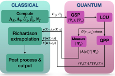
Figure 1: The figure shows the working flowchart of the hybrid quantum-classical algorithm. The quantum circuit and system parameters are first computed classically and then loaded on the quantum device using quantum state preparation. The forward time simulation is then performed using the algorithm on the linear combination of unitaries. The solutions are then either post-processed quantumly or measured for storage on a classical device. This process is iterated over several times and the measured information is extrapolated classically using Richardson extrapolation, to finally output the solution.

(1) Four unitaries: A non-unitary matrix $M$ can be decomposed into symmetric and anti-symmetric matrices, $S$ and $A$, respectively, as

$$S =\frac{1}{2}(M+M^{{\dagger}})~{}\text{\&}$$ (4)

$$A =\frac{1}{2}(M-M^{{\dagger}}),$$ (5)

where $M=S+A$. Each of these matrices can be further decomposed exactly as

$$S =\lim_{\epsilon\rightarrow 0}\frac{i}{2\epsilon}(e^{-i\epsilon S}-e^{i\epsilon S})$$ (6)

$$A =\lim_{\epsilon\rightarrow 0}\frac{1}{2\epsilon}(e^{\epsilon A}-e^{-\epsilon A}),$$ (7)

where $\epsilon$ is an expansion parameter. It can be easily shown that $e^{\pm iS}$ and $e^{\pm A}$ are both unitary matrices. We shall now define these operators as $U_{0}=ie^{-i\epsilon S}$, $U_{1}=-ie^{i\epsilon S}$, $U_{2}=e^{\epsilon A}$ and $U_{3}=-e^{-\epsilon A}$, and express $M$ exactly as a weighted sum of purely unitary operators given by $M=\sum_{k=0}^{k=3}\beta_{k}U_{k}=\lim_{\epsilon\rightarrow 0}\frac{1}{2\epsilon}(U_{0}+U_{1}+U_{2}+U_{3})$. However, in practice, we approximate $M$ by choosing a small enough $\epsilon$, thus resulting in a decomposition with just 4 unitaries given by

$$\tilde{M}=\frac{1}{2\epsilon}(U_{0}+U_{1}+U_{2}+U_{3}).$$ (8)

Since the goal is to be able to simulate our algorithms on NISQ and near-term devices, it is desired to have a reduction in circuit depth. We now show that we can go a step further to reduce this decomposition to only two unitaries.

(2) Two unitaries: We can attain this reduction by trading in one extra qubit. For this, consider a simple hermitian dilation of the original matrix $M$ given by

$$\hat{M}=\begin{pmatrix}0&M\\ M^{{\dagger}}&0\end{pmatrix}.$$ (9)

Since $M_{ij}\in\mathbb{R}$, the matrix $\hat{M}$ is symmetric with zero anti-symmetric part. This would leave us with a symmetric, hermitian, and Hamiltonian $\hat{M}$ that can be decomposed into just two unitaries as

$$\hat{M}=\lim_{\epsilon\rightarrow 0}\frac{i}{2\epsilon}(e^{-i\epsilon\hat{M}}-e^{i\epsilon\hat{M}})=\frac{1}{2\epsilon}(\hat{U}_{0}+\hat{U}_{1}).$$ (10)

However, to accommodate this reduction, the size of input vector would need to be doubled and given by $\hat{b}=[0,b]$, where one half of the dilated vector is padded with zeros. This doubling would require only one additional qubit. From here on, let $K$ represent the number of unitaries corresponding to either two or four unitaries. We now examine how to implement the decomposition as a quantum circuit.

The basic circuit requires two quantum registers, both set to 0 initially: (1) $|\Psi\rangle_{u}$ – to store the state vector that is to be operated on, and (2) $|\Psi\rangle_{a}$ – a register with a total of $n_{a}=\log_{2}(K)$ ancillary qubits (here, $n_{a}\in\{1,2\}$). $|\Psi\rangle_{u}$ is prepared using the operator $R$ which, in our case, is simply a NOT gate to prepare the initial delta function. $|\Psi\rangle_{a}$, on the other hand, is prepared by an operator $V$ into a superposition state proportional to

$$|\Psi\rangle_{a}=V|0\rangle^{\otimes n_{a}}=\sqrt{1/\beta}\sum_{k}\sqrt{\beta_{k}}|k\rangle,$$ (11)

where $\beta=\sum_{k}\beta_{k}$. Since all $|\beta_{k}|$ are equal, the ancillary register can be prepared as a uniform superposition state by simply applying Hadamard gates on each qubit of the register. This preparation step is also efficient, since it requires only an $\mathcal{O}(1)$ depth operation. Now, using register $|\Psi\rangle_{a}$ as the control qubits, we apply the LCU unitaries as a series of uniformly controlled operations $U_{k}$ on $|\Psi\rangle_{u}$ which is represented by the operator, $W=\sum_{k}|k\rangle\langle k|\otimes U_{k}$. Then, $|\Psi\rangle_{a}$ is reset to 0 by applying $V^{{\dagger}}$. Finally the ancillary register is measured in the computational basis, yielding a state proportional to

$$|\Psi\rangle =R|0\rangle^{\otimes n_{a}}\otimes V|0\rangle^{\otimes n_{g}}\mapsto(V^{{\dagger}}\otimes\mathbb{I})\otimes W(|\Psi\rangle_{a}\otimes|\Psi\rangle_{u})$$

$$=|0\rangle^{n_{a}}\Big{(}\sum_{k}\beta_{k}U_{k}\Big{)}|\Psi\rangle_{u}+|\Psi\rangle_{\perp}$$

$$=\frac{1}{\sqrt{\beta}}|0\rangle^{n_{a}}M|\Psi\rangle_{u}+|\Psi\rangle_{\perp}.$$ (12)

Here, we drop for brevity the normalization constants as may exist, $|\Psi\rangle_{\perp}$ corresponds to an orthogonal subspace that stores the unwanted remainder from the above operation of eq. (8). The post-selected solution subspace is then re-scaled classically by $\mathcal{O}(|||\Psi\rangle_{u}||/\epsilon)=\mathcal{O}(1/\epsilon)$ to obtain the actual solution. However, this procedure also shows that, the circuit for linearly combining the unitaries applies the operator $M$ only probabilistically, and the solution subspace of the quantum state is prepared with a small but finite success probability $p_{\textrm{succ}}$. Since we are interested in applying such a decomposition for $\tau$ time steps, $p_{\textrm{succ}}$ would decay as function of $f(2^{-K},\epsilon^{-1},\tau,|||\Psi\rangle_{\tau}||^{-1})$. The smaller the $p_{\textrm{succ}}$, the larger is the number of repeated circuit simulations (query complexity or shots) required to measure or sample the solution subspace accurately. However, we design the time marching quantum circuits such that the overall query complexity is still kept near optimal, such that the required number of shots does not blow up exponentially. For instance, we use a Richardson extrapolation strategy (outlined in Section V), with which we can do simulations even when $\epsilon\sim\mathcal{O}(1)$.

Finally, to translate these operations outlined above into quantum circuits that work on simulators or real hardware, one would need a further decomposition of the above operators into fundamental 1- and 2-qubit gates. This can be done in one of the following ways.

(a) Direct Approach – This involves decomposing the controlled multi-qubit unitaries into standard two-level unitaries, which in turn require about $\mathcal{O}(N^{2})$ 2-qubit gates [barenco1995elementary, nielsen2010quantum]. Such a decomposition results in deep circuits that might be amenable only on future fault-tolerant devices. Although the chances of achieving a quantum advantage from such a decomposition are bleak to none at present, one could still attempt to use circuit parallelization strategies, proposed in Section V, to ameliorate the large circuit depths. Additionally, since the current decomposition requires only two controlled-unitaries, this reduces the overall circuit depth further, compared to previously proposed unitary methods.

(b) QISKIT Transpile – IBM’s quantum simulators offer an optimized transpile functionality (a culmination of various underlying algorithms), that decompose multi-qubit unitaries into single and two qubit gates, picked from a fixed basis of gates available. These transpliations offer multiple levels of optimization with which the circuit depths can be further shortened. This also allows one to design circuits by considering a specific qubit topology on a quantum processor, to extract the best performance. The transpilation feature is quite robust if not the most efficient. We use this feature to implement our linear unitary circuits to conduct real IBM hardware experiments and perform noisy simulations with Qiskit Aer, the results of which are described in Section LABEL:sec:_Numerical_results.

(c) Hamiltonian Simulation – To analyze theoretically the asymptotic gate complexity scaling of the proposed algorithms (in terms of 1- and 2-qubit gates), we assume access to a black-box with simulations based on Hamiltonian algorithm (described in [berry2015hamiltonian] (see Lemma 10) and [childs2017quantum] (see Sec. 2.1, Lemma 8 and proof of Theorem 3 in Sec. 3.1)), to efficiently implement the controlled unitaries. In our case, this translates to implementing a Hamiltonian simulation of unitaries of the form $e^{\pm i\epsilon\hat{S}}$ (for $K=2$) and its powers. For an $s-$sparse matrix $\hat{M}$, of size $N\times N$, scaled such that $||\cdot||\leq 1$, the gate complexity to implement controlled unitaries of the form $e^{\pm i\epsilon\hat{S}}$, up to an admissible error of $\varepsilon_{U}$, would require

$$G_{U}=\mathcal{O}\big{(}(s\epsilon+1)(\log N+\log^{2.5}(\epsilon/\varepsilon_{U}))\log(\epsilon/\varepsilon_{U})\big{)}$$ (13)

one- and two-qubit gates [berry2015hamiltonian]. From here on, $G_{U}$ represents the above expression. We remark here that the sparsity is $s=d+2$, where $d$ is the order of finite central difference scheme used. Even if we pick an extremely accurate scheme with the order $d=8$, say, the sparsity would at most be $s=10$, thus contributing only a small pre-factor to the above asymptotic complexity.

IV Time marching compact quantum circuits

As already mentioned, a time marching numerical scheme can be translated into one of the following operations: $\mathbf{u}(\mathbf{x},t+1)=A\mathbf{u}(\mathbf{x},t)$ or $=A^{-1}\mathbf{u}(\mathbf{x},t)$, which are called explicit and implicit schemes, respectively (see Section LABEL:sec:_Numerical_Setup of the Appendix). For the present discussion, the general matrix $M$ used before will be replaced by $A$, which now represents a specific numerical setup. We wish to use the framework of linear combination of unitaries, developed in the previous section, to perform efficient time marching simulations, using the above two matrix operations. We now introduce six methods of constructing quantum circuits to perform such a simulation. We shall refer to these as Time Marching Compact Quantum Circuits (TMCQC1-6) and outline their designs. In the discussion immediately below, we make an implicit assumption—which we discuss in more detail towards the end of this section—that the query complexity required to reconstruct the final solution contributes a constant pre-factor to the overall complexity of each method, thus making comparisons between gate complexities and classical time complexities more meaningful.

IV.1 TMCQC1 - Explicit Expansion Circuit

With explicit time marching (see Section LABEL:subsec:_Explicit_TMCQC of the Appendix), integrating the system for $\tau$ time steps requires the application of matrix-vector multiplication operations of the form $(\mathbf{A}_{E})^{\tau}$. In TMCQC1, such an operator is approximated either by two or four unitaries by naively computing the multinomial expansion given by (we drop the $1/(2\epsilon)$ for brevity),

$$(\mathbf{A}_{E})^{\tau}=\Big{(}U_{0}+U_{1}+U_{2}+U_{3}\Big{)}^{\tau}\textrm{~{}~{}or~{}~{}}=\Big{(}\hat{U}_{0}+\hat{U}_{1}\Big{)}^{\tau}$$

$$\implies\sum_{|v|=\tau}{\tau\choose v}U^{v}\equiv\sum_{k=0}^{N_{T}-1}\tilde{U}_{k},$$ (14)

where $v=(v_{1},\cdots,v_{K})$ and $U^{v}=U^{v_{1}}_{0}U^{v_{2}}_{1}\cdots U^{v_{K}}_{K-1}$.

Gate complexity - This multinomial expansion with $K$ monomials has a total of $N_{T}=$$\tau+K-1\choose K-1$ terms. When $K=2\textrm{~{}or~{}}4$, $N_{T}=$ $\mathcal{O}(\tau)$ or $=\mathcal{O}(\tau^{3})$, respectively. For the rest of the section, we shall use $K=2$ for clarity. Now each term in the above expansion is in turn a product of at most $\mathcal{O}(\tau)$ unitaries. Therefore the overall expansion has at most of $\mathcal{O}(\tau^{2})$ unitaries in total. We shall refer to this as the LCU depth. From the previous section we know that, each of these unitaries can be implemented with a gate complexity of $G_{U}$ at best, thus giving a total complexity of $\mathcal{O}(G_{U}\tau^{K})\equiv\mathcal{O}(\log(N_{g}),\textrm{polylog}(\epsilon/\varepsilon_{U}),s\epsilon,\tau^{2})$. Now, comparing this with the classical complexity of explicit time marching via simple matrix-vector multiplications, given by $\mathcal{O}(N_{g}s\tau)$ [shewchuk1994introduction], we may infer the following. The quantum algorithm is exponentially better in $N_{g}$, but worse in $\tau$ by $\mathcal{O}(\tau)$. This implies that, even though the quantum algorithm is exponentially better in $N_{g}$, in order to compensate for the $\tau$ scaling, one would need to set the CFL stability criterion such that $N_{g}\gg\tau$; this ensures that the advantage gained by the $N_{g}$ scaling outperforms (or at the least matches the loss from) the poorer $\tau$ scaling. In any case, it would suggest that simulating only short $T$ horizons would make this step possible. Further, if we had access to (say) $\mathcal{O}(\tau)$ parallel circuits, we could simulate the unitaries in parallel (as discussed later in Sec. V) to lower the gate complexity, thus ameliorating the $\tau$ scaling.

Qubit complexity - This approach would require $n_{a}=\log_{2}(\tau)$ ancillary qubits, $n_{g}=\log_{2}(N_{g})$ qubits to store the velocity field, giving a total of $n=\log_{2}(N_{g}\tau)$ qubits.

IV.2 TMCQC2 - Explicit Serial Circuit

The previous approach can be improved by trading in a few extra qubits, while still keeping the total qubit complexity logarithmic in the problem size. An alternative way to implement the same operation as earlier is to concatenate the LCU decomposition of $A_{E}$ serially, $\tau$ times. However, to keep track of the time steps, we would need an additional register, which we shall refer to as clock register, comprising $n_{c}=\log_{2}(\tau)$ qubits. The quantum circuit for this is shown in figure 2(a) (for $K=4)$. A step-by-step description of this circuit operation is outlined in Section LABEL:subsec:_Explicit_TMCQC of the Appendix.

Gate complexity - It is easy to see that a serial circuit such as this would lead to an LCU depth of $\mathcal{O}(\tau)$, with a total gate complexity of $\mathcal{O}(G_{U}\tau)\equiv\mathcal{O}(\log(N_{g}),\textrm{polylog}(\epsilon/\varepsilon_{U}),s\epsilon,\tau)$. Comparing this with the classical scaling of $\mathcal{O}(N_{g}s\tau)$, one is led to conclude that the quantum algorithm is exponentially better in $N_{g}$ and comparable in $\tau$ and $s$, thus offering a potential advantage for any $\tau\geq 1$.

Qubit complexity - It is clear that the number of qubits required in this case is $n=n_{g}+n_{a}+n_{c}=\log_{2}(N_{g}\tau)+2$.

IV.3 TMCQC3 - Implicit Expansion Circuit

We now consider an implicit time marching scheme, which requires one to perform matrix inversion operations. Since we are now faced with an inversion problem, decomposing by linear combination of unitaries is more involved. Some approaches proposed earlier include approximating the inverse function $f(x)=1/x$, in terms of either Fourier or Chebyshev series [childs2017quantum]. The terms in these series are then implemented as unitary gates. Alternatively, we explore here a simpler yet efficient approach by truncating a Neumann series expansion to approximate a matrix inverse operation of the form $\mathbf{A}_{I}=(\mathbf{I}-\alpha\mathbf{A})^{-1}$. The series approximation up to $P$ terms could be written as $(\mathbf{I}-\alpha\mathbf{A})^{-1}=\sum_{p=0}^{P}\mathbf{A}^{p}\approx\tilde{\mathbf{A}}_{I}$, where $\tilde{\mathbf{A}}_{I}$ represents the approximate inverse operator. The accuracy of this approximation is given by the truncation error $\varepsilon_{N}$, which clearly depends on the number of terms retained in the series. A detailed account of this method is presented in Section LABEL:sec:_Trunc_Neumann_Series of the Appendix, where Lemma 1 proves this result: Given an $\alpha$ such that the spectral radius $\rho(\mathbf{\alpha A})<1$ (to ensure convergence), and if $P_{min}$ is the number of terms for a truncation error of $\varepsilon_{N}$, the error is bounded from above as

$$\varepsilon_{N}\leq\mathcal{O}\big{(}||\mathbf{A}||^{P_{min}}\big{)}=\mathcal{O}((\kappa-1)^{P_{min}}).$$ (15)

From this, it can be easily shown that the number of terms required is

$$P_{min}=\mathcal{O}\Bigg{(}\Bigg{\lceil}\frac{\log(1/\varepsilon_{N})}{\log(1/||\mathbf{A}||)}\Bigg{\rceil}\Bigg{)}=\mathcal{O}\Bigg{(}\Bigg{\lceil}\frac{\log(1/\varepsilon_{N})}{\log(1/(\kappa-1))}\Bigg{\rceil}\Bigg{)}.$$ (16)

From Proposition 2 of the Appendix, it is also clear that the error in the velocity solution obtained from such a truncated approximation is similarly bounded. Each term of the truncated series is now further decomposed, using the linear combination unitary method. The final set of unitaries is obtained by computing the multinomial expansion of the new truncated series, while marching forward $\tau$ time steps.

Gate complexity - To compute the gate complexity, first consider a $p$^th order term in the truncated series. If this term is written in terms of the unitaries decomposition, it will produce $p+K-1\choose K-1$ terms, which is $\mathcal{O}(p^{K-1})$. Recall that each of these newly produced terms is in fact a product of $p$^th order products (at most) of unitaries, thus making the depth $\mathcal{O}(p^{K})$. Next, we sum the series up to $P_{min}$ terms, giving a total of (for $K=2$) $\mathcal{O}(P^{3}_{min})$. Finally, since we need to perform time marching, the series obtained above is finally raised to the exponent $\tau$, expanding which gives a total depth of $N_{T}=$${\tau+(P^{\text{min}})^{3}-1\choose(P^{\text{min}})^{3}-1}=\mathcal{O}(\tau^{P^{3}_{min}})$. Therefore the overall gate complexity is $\mathcal{O}(G_{U}\tau^{P^{3}_{min}})$. It is clear that the algorithm is exponential in $\tau$ and also clearly worse (in terms of $\tau$) than the corresponding classical complexity given by $\mathcal{O}(\log(N_{g}s\tau\kappa\log(1/\varepsilon)))$. Again, although the algorithm is still logarithmic in $N_{g}$, it offers the poorest complexity scaling compared to all other TMCQCs presented here.

Qubit complexity - We note that this algorithm requires $n_{g}=\log_{2}(N_{g})$ qubits for storing the grid, $n_{a}=P^{3}_{min}\log_{2}(\tau)$ ancilla qubits for the LCU decomposition, thus giving a total qubit complexity of $\mathcal{O}(P^{3}_{min}\log(N_{g}\tau))$.

Although we will show that the current method TMCQC3 offers the poorest complexity scaling among the algorithms discussed, the benefit of the Truncated Neumann Series approach will be reaped maximally by the algorithms to be described next.

IV.4 TMCQC4 - Implicit Serial Circuit

We can improve the previous algorithm by using an additional clock register. The set of unitaries obtained from the truncated Neumann series is now concatenated serially $\tau$ times to perform time marching, with the clock register tracking the time step count.

Gate complexity - The truncated series has a total of $\mathcal{O}(P^{3}_{min})$ terms, so the total depth can be estimated to be $\mathcal{O}(P^{3}_{min}\tau)$. Thus it can be seen readily that the total gate complexity is $\mathcal{O}\Big{(}s\epsilon,\log(N_{g}\tau),\textrm{polylog}(\epsilon/\varepsilon_{U},1/\varepsilon_{N}),\log^{-3}((\kappa-1)^{-1})\Big{)}$. Comparing this with the classical complexity of $(\log(N_{g}s\tau\kappa\log(1/\varepsilon)))$, one finds that the algorithm (without any parallelization) has a comparable scaling in $\tau$, while it is exponentially better than classical in $N_{g}$ and $\kappa$.

Qubit complexity - It can be seen easily that this approach has the total qubit complexity of $\mathcal{O}(\log(N_{g}\tau P_{min}))$.

IV.5 TMCQC5,6 - Explicit & Implicit One-shot Circuits

Now two final quantum circuit designs are described; as we shall show, they offer the most efficient complexity scaling so far. In contrast to previous methods, these approaches construct a single-large matrix inversion problem (of the size $N_{g}\tau\times N_{g}\tau$), solving which provides at once the solutions for all time steps and hence the term one-shot. (This should not be confused with the number of shots required to sample the wavefunctions). This method can be constructed with both explicit ($\mathbf{A}_{EO}\tilde{u}=\mathbf{b}_{EO}$) or implicit ($\mathbf{A}_{IO}\tilde{u}=\mathbf{b}_{IO}$) schemes; details of these construction are outlined in the Appendix. In order to approximate the inverse, we again use the truncated Neumann series as in TMCQC3,4. Since in this case the solution of the matrix inversion includes the solutions at all time steps, there is no need for any further action. The terms of the truncated series can now be readily written in terms of the unitaries decomposition. Furthermore, since the method avoids an iterative/serial style time marching, the diminution of success probability is also less severe than in previous methods. Gate complexity - This is given by simply computing the terms obtained by just applying the unitaries decomposition to each term of the truncated series. The depth is therefore just $\mathcal{O}(P^{3}_{min})$, which yields a total gate complexity of $\mathcal{O}(G_{U}P^{3}_{min})\equiv\mathcal{O}\Big{(}s\epsilon,\log(N_{g}\tau),\textrm{polylog}(\epsilon/\varepsilon_{U},1/\varepsilon_{N}),\log^{-3}((\kappa-1)^{-1})\Big{)}$. This scaling is nearly optimal in every parameter except $s$, which, as already noted earlier, is at most $s\leq 10$. Thus the method is exponentially better than its classical counterpart in terms of all system parameters.

Qubit complexity - The input vector is now a larger dimensional state of size $N_{g}\tau$, which requires $n_{g}=\log_{2}(N_{g}\tau)$ qubits. Further, to apply the unitaries decomposition, we require an ancilla register of size $n_{a}=3\log_{2}(P_{min})$ thus having a total qubit complexity of $\mathcal{O}(\log_{2}(\tau N_{g}P_{min}))$.

The complexities of all circuit designs discussed above are summarized in Table IV.5.

Table 1: Summary of computational complexity of quantum algorithms

c—c—c—c—c [tikz=top color=olive!25]*-1 [tikz=top color=teal!35]*-2 [tikz=top color=teal!30]*-2 [tikz=top color=teal!25]*-1 [tikz=top color=teal!20]*-1
Algorithm LCU depth Gate complexity Classical complexityQubit complexity


QSP - $\mathcal{O}(2kn)$ -$\mathcal{O}(\log(N_{g}))$
^{[bharadwaj2023hybrid, mozafari2022efficient]}
Explicit

TMCQC1 $\mathcal{O}\big{(}\tau^{2}\big{)}$ $~{}\mathcal{O}\Big{(}s\epsilon,\log(N_{g}),\textrm{polylog}(\epsilon/\varepsilon_{U}),\tau^{2}\Big{)}~{}$ $\mathcal{O}(N_{g}s\tau)$$\mathcal{O}(\log(N_{g}\tau))$

TMCQC2 $\mathcal{O}\big{(}\tau\big{)}$ $~{}\mathcal{O}\Big{(}s\epsilon,\log(N_{g}),\textrm{polylog}(\epsilon/\varepsilon_{U}),\tau\Big{)}~{}$ $\mathcal{O}(N_{g}s\tau)$$\mathcal{O}(\log(N_{g}\tau))$

TMCQC5 $\mathcal{O}\big{(}P_{min}^{3}\big{)}$ $~{}\mathcal{O}\Big{(}s\epsilon,\log(N_{g}\tau),\textrm{polylog}(\epsilon/\varepsilon_{U},1/\varepsilon_{N}),\log^{-3}((\kappa-1)^{-1})\Big{)}~{}$ $\mathcal{O}(N_{g}s\tau\kappa\log(1/\varepsilon))$ $\mathcal{O}(\log(N_{g}\tau P_{min}))$

Implicit

TMCQC3 $\mathcal{O}\Big{(}\tau^{P_{min}^{3}}\Big{)}$ $~{}\mathcal{O}\Big{(}s\epsilon,\log(N_{g}),\textrm{polylog}(\epsilon/\varepsilon_{U}),\tau^{P_{min}^{3}}\Big{)}~{}$ $\mathcal{O}(N_{g}s\tau\kappa\log(1/\varepsilon))$$\mathcal{O}\big{(}P^{3}_{min}\log(\tau N_{g})\big{)}$

TMCQC4 $\mathcal{O}\big{(}\tau P^{3}_{min}\big{)}$ $~{}\mathcal{O}\Big{(}s\epsilon,\log(N_{g}\tau),\textrm{polylog}(\epsilon/\varepsilon_{U},1/\varepsilon_{N}),\log^{-3}((\kappa-1)^{-1}),\tau\Big{)}~{}$ $\mathcal{O}(N_{g}s\tau\kappa\log(1/\varepsilon))$ $\mathcal{O}\big{(}\log(\tau N_{g}P_{min})\big{)}$

TMCQC6 $\mathcal{O}\big{(}P_{min}^{3}\big{)}$ $~{}\mathcal{O}\Big{(}s\epsilon,\log(N_{g}\tau),\textrm{polylog}(\epsilon/\varepsilon_{U},1/\varepsilon_{N}),\log^{-3}((\kappa-1)^{-1})\Big{)}~{}$ $\mathcal{O}(N_{g}s\tau\kappa\log(1/\varepsilon))$$\mathcal{O}\big{(}\log(\tau N_{g}P_{min})\big{)}$

QPP - $\mathcal{O}(U_{V})+\mathcal{O}((\log N)^{2}/\epsilon_{QPP})$ - varies
^{[bharadwaj2023hybrid]}

IV.6 Query complexity and success probability

The gate complexities outlined above correspond to a single application of the quantum circuit. However, the solution thus prepared has a small, yet finite success probability $p_{\textrm{succ}}$. This implies that one would need to query the circuit repeatedly (in other words, repeat the experiment for $N_{s}$ shots) to reconstruct the solution state by repeated sampling. The overall time complexity of the simulation would therefore be the product of the gate and query complexities. To compute this, we need to first estimate $N_{s}$ for which we first consider eq. (12) that represents the fundamental action of linear unitaries. Before rescaling the solutions, simply applying the unitaries circuit prepares the state proportional to $2\epsilon A|\Psi\rangle$. From Proposition 1 (see Appendix), without loss of generality, the matrix $A$ can always be scaled by a small constant $\delta\lesssim\mathcal{O}(1/\epsilon)$, and the solutions can be simply scaled back after measurements. Therefore the solution subspace produced from eq. (12) can be said to be proportional to $(2\epsilon\delta/\sqrt{\beta})A|\Psi\rangle.$ This implies that a single application of the linear unitaries operation produces the desired state with the success probability

$$p_{\textrm{succ}}\sim\Bigg{(}\frac{2\epsilon\delta||A|\Psi\rangle||}{\sqrt{\beta}}\Bigg{)}^{2}.$$ (17)

The above value is for a single linear combination of unitaries block. However in essence, each TMCQC provides a different unitary block-encoding of the corresponding $A$ to perform time marching. The $p_{\textrm{succ}}$ of the solution at $t=\tau\Delta t$ thus varies for each TMCQC. The specific dependence arises from the difference in the number of times the unitaries oracle is queried and the corresponding depth, which we shall represent from now on as $G_{\textrm{L}}$. Comparing all the TMCQCs we can easily identify that in TMCQC2 and TMCQC4, the decay in $p_{\textrm{succ}}$ is particularly the most severe since the unitaries are applied in series. Therefore for $\tau$ such applications, the RHS of eq. (17) will now be raised to the power $\tau$. For generality, let us represent this exponent with $G_{\textrm{L}}$. A single application of the two-unitary oracle involves preparing a superposition state by Hadamard gates acting on ancilla qubits. This implies that $\beta=2$. Since the $p_{\textrm{succ}}$ for every time step is independent, the probability thus tends to decay exponentially [berry2022quantum, fang2023time], compounding for each of the $\tau$ steps. Apart from this, the overall success probability also depends on ratio of the norms of the initial and final time solution states. Thus, we can rewrite $p_{\textrm{succ}}$ as

$$p_{\textrm{succ}} =\Bigg{(}\frac{2\epsilon\delta||A||}{2}\Bigg{)}^{2G_{\textrm{L}}}\prod_{k=1}^{G_{\textrm{L}}}\frac{||~{}|\Psi\rangle_{k}~{}||^{2}}{||~{}|\Psi\rangle_{k-1~{}}||^{2}}$$

$$=(\epsilon\delta||A||)^{2G_{\textrm{L}}}\frac{||~{}|\Psi\rangle_{\tau}~{}||^{2}}{||~{}|\Psi\rangle_{0}~{}||^{2}}.$$ (18)

This implies that it would require at least

$$N_{s}=\Bigg{(}\frac{1}{\epsilon\delta||A||}\Bigg{)}^{2G_{\textrm{L}}}\frac{||~{}|\Psi\rangle_{0}~{}||^{2}}{||~{}|\Psi\rangle_{\tau}~{}||^{2}}\approx\mathcal{O}\Bigg{(}\frac{||~{}|\Psi\rangle_{0}~{}||^{2}}{||~{}|\Psi\rangle_{\tau}~{}||^{2}}\Bigg{)}$$ (19)

number of shots to recover the solution, up to a constant pre-factor $\eta^{2G_{\textrm{L}}}=(1/\epsilon\delta||A||)^{2G_{\textrm{L}}}$. Since we can readily choose an $\epsilon$ and $\delta$ such that $\epsilon\delta||A||\gtrsim 1$ (see Proposition 1 of Appendix and its ensuing discussion), such that $\eta\sim\mathcal{O}(1)$ is not an unfavorably large constant; this takes the overall complexity closer to optimal.

We should also note that the complexity discussed above can be further improved quadratically by applying a Grover-like amplitude amplification, as shown in [brassard2002quantum]. However, we continue our discussion without it, to emphasize that the corresponding results are still efficient in some strict sense, even before applying amplitude amplification. This optimistic nature of the discussion can however be quickly diminished when we begin to consider the effects of noise. In practice (as shown later in Section LABEL:sec:_Numerical_results), to simulate these circuits on currently available IBMQ machines, we need at least $N_{s}=2^{15}$ shots to be able to accurately recover the solution. Nevertheless, the query complexity presented here relates to the asymptotic complexity scaling, which suggests that, when reasonably large problem sizes are solved with the proposed methods, the required shot count will not significantly diminish any available quantum advantage.

In summary, it is ideal to ensure that $\eta\lesssim 1$, otherwise it would lead to a large pre-factor $\mathcal{O}(2^{\log(\tau)/\log(\kappa-1)})$ at best, or $\mathcal{O}(2^{\tau^{2}})$ at worst. While ensuring the query complexity to be controllable, the following three situations need special attention.

1. Stability criteria – Flow problems solved by implicit schemes (TMQCQ3,4,6) are not constrained by any stability criteria, which therefore allows more flexibility to choose the parameters. However, explicit schemes as in TMCQC1,2,5 have to satisfy a stability criterion. For the specific case of the advection-diffusion problem being discussed, this is equivalent to $\alpha=D\Delta t/(\Delta x)^{2}\leq 0.5$. This criterion requires the system parameters $U,N_{g},\Delta t$ to be chosen to satisfy $\delta||A||<1$ and $\delta\epsilon||A||\gtrsim 1$. For second-order, central difference, explicit scheme, $||A||=1$. In this case, just ensuring $\delta\epsilon\gtrsim 1$ is sufficient.

2. Noise – As already noted, it is important to choose a large enough $\epsilon$ to make the solution distinguishable from noise. At the same time, to maintain the accuracy of the solution even for large $\epsilon$ values, we could employ the concept of Richardson-extrapolation to defer our approach to $\lim\epsilon\rightarrow 0$. The accuracy of the extrapolated solutions can be $\mathcal{O}(\epsilon^{4})$ or better. Viewed alternatively, we can lower the shot count $N_{s}$ significantly for the same given accuracy.

3. Steady state and decaying flows – The above two considerations alone are insufficient to maintain a small $N_{s}$. We also need to ensure that the steady state limit

   $$\lim_{\tau\rightarrow\infty}\frac{||~{}|\Psi\rangle_{0}~{}||}{||~{}|\Psi\rangle_{\tau}~{}||},$$

   does not diverge. If the time marching operator is norm-preserving (or the flow is statistically steady), then $||~{}|\Psi\rangle_{\tau}~{}||=||~{}|\Psi\rangle_{0}~{}||$ trivially. The alternative scenario of the norm-increasing flow is better, where $||~{}|\Psi\rangle_{\tau}~{}||\geq||~{}|\Psi\rangle_{0}~{}||$, corresponding to flows that experience constantly increasing net influx of energy. Both cases are in practice possible if we consider a constant forcing term in our governing PDEs. However, the more restrictive case is the viscous, dissipative flow whose norm decays with time; in this case the steady state of the flow corresponds to vanishingly small velocity fields due to constant dissipation of energy from the system. However, the advection-diffusion problem considered in this work is not as severe as can be seen from the analytical solution [ingelmann2023two]. The steady state corresponds to a constant, uniform velocity field with a small, yet non-zero norm (in this work, this ratio is = 1/2). For flows whose steady state norms are identically zero, the query complexity grows as $\mathcal{O}(||~{}|\Psi\rangle_{\tau}~{}||^{-1})$. In such cases, there could be two alternatives (which should be studied in more detail): (1) The problem of the growing pre-factor $\eta$ can be addressed by choosing a smaller $\epsilon$ such that $\eta^{G_{\textrm{L}}}\sim\mathcal{O}(||~{}|\Psi\rangle_{\tau}~{}||^{-1})$. (2) When this choice is not possible, one is limited to solving the problem for only short time horizons, for which the norm decays not too steeply.

   The scenario described so far considers the growth in $N_{s}$ as being most severe. If, however, we consider TMCQC5,6 there is no compounding decay in terms of $\epsilon$. The only contributing factor would be from the normalization stemming from the linear decomposition in terms unitaries. However, we show that the unitaries depth is $\mathcal{O}(\log(1/\epsilon)/\log(1/(\kappa-1))^{3}$. For large problem sizes, the corresponding pre-factor in query complexity would not be critical. In any case, from the discussion so far, it is clear that the overall time complexity of the algorithms can be pushed closer to optimal.

V End-to-end algorithm and near-term strategies

A hybrid quantum-classical algorithm requires one to consider: (A) a suitable quantum state preparation, (B) an optimal circuit design for the quantum solver, (C) efficient solution read-out and post processing, and (D) effects of noise and decoherence on real quantum hardware. These factors tend to diminish expected quantum advantage. In this section we outline strategies that could potentially render the overall algorithm to be an end-to-end type, as well as one that can be simulated on noisy near-term quantum devices, while retaining some quantum advantage. A schematic of these methods and typical circuit designs are given in figure 2(b).

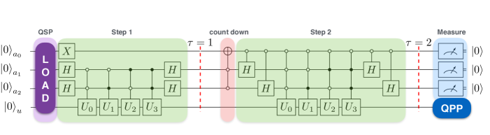
(a)

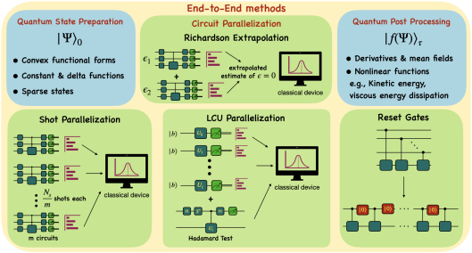
(b)

Figure 2: (a) 4 qubit iterative LCU circuit to implement a simulation for $\tau=2$ time steps is shown. Here the first register $q(a_{0})$ is the counter qubit, which is initially set to one and successively bit-flipped to count the time steps in a binary fashion. The ancilla qubits $q(a_{1})$ and $q(a_{2})$ are required to implement the linear combination of four unitaries $U_{0}$ to $U_{4}$. The last register $q(u)$ stores the velocity field at every time step. (b) Schematic of the end-to-end strategies and their quantum circuits that can be used to preserve potential quantum advantage.

(1) Quantum State Preparation - The first step of a hybrid QCFD algorithm is to encode the initial velocity field into qubit states. In general, for arbitrary states of size $N$, the complexity of state preparation would scale linearly with $N$. This scaling compromises the quantum speed-up that might be achieved from the PDE solver algorithm. However, specific examples might not need such exponential circuit depths. For an input state that has an integrable, convex functional form, the initial state can be prepared with sub-exponential circuit depths as shown in [grover2002creating, vazquez2022enhancing, bharadwaj2023hybrid]. For sparse states, one can prepare the initial state more efficiently with sub exponential circuit depths [mozafari2022efficient, zhang2022quantum, bharadwaj2023hybrid]. Certain cases might, however, require one to trade additional ancillary qubits for shorter circuit depths. Further, since the algorithms proposed here require only a single copy of the initial state for every circuit execution, we can begin with a simple state that is easy to prepare. In fact, most problems in fluid dynamics offer great flexibility in choosing initial conditions, which could be a uniform flow (constant function) that would require a state preparation circuit of just a single layer of Hadamard gates, or a delta function (the case considered here), preparing which requires a single NOT gate. Many times, a random initial conditions are admissible or necessary. More recent efforts demonstrate efficient ways to encode polynomial functions as well [gonzalez2024efficient].

(2) Circuit Parallelization and Reset gates - Circuit depths that can be simulated on current and near-term hardware are rather limited. The limitation arises from the finite, short coherence life-spans of the qubits. Longer circuit executions tend to run into errors based on decoherence. In order to make an attempt at fitting the TMCQCs on such hardware, we propose here a few strategies to parallelize the circuit execution, to both reduce the effective circuit depths and the execution times.

(A) Shot parallelization - Generally the shot count available on real quantum hardware (here, IBMQ) is limited to about $\sim 2^{15}\textrm{~{}to~{}}2^{19}$ shots. If we consider a simulation requiring a large shot-count of about (say) $N_{s}=2^{20}$ shots or higher, such an execution would not be possible with current hardware. A simple workaround to achieve this would be actually to execute multiple quantum circuits in parallel. For the current example, naively, we can perform two parallel circuit executions with $2^{19}$ shots each. When possible, we could go even further by executing several low shot-count circuits in parallel, with which we can increase the total shot count while improving the sampling accuracy of the quantum state. To fit our simulations using only the available shot count, we could instead use the Richardson extrapolation to lower the required $N_{s}$. This is discussed below in this section.

(B) LCU parallelization - Let us consider a single time step simulation using either two or four unitary block encoding.

1. Naive Parallel unitaries - We execute each unitary $U_{i}$ (without any controls) in parallel on 2 (or 4) separate circuits, starting with the same initial state. This requires $3n_{g}$ qubits in total. When the resulting parallel (partial) solution states have purely real amplitudes, we can perform a straightforward measurement in the computational basis of each partial solution. Following this, these partial solutions can be combined classically to output the final solution. However, if any of the partial solutions have complex amplitudes, a direct extraction of solutions requires expensive tomography to reconstruct the state. Two possibilities exist. In the first case, we combine those parallel unitaries as a single circuit such that the grouping produces real amplitudes for the partial states. From here, we can proceed with measurement as earlier. This new grouping would, of course, increase the depth of the circuit, which is now at some intermediate level of parallelization. Secondly, if we are interested only in computing the expectation value of a certain observable, instead of the full state, it can be done while still retaining the full parallelization. The expectation value of an operator $U_{i}$ can be computed accurately by using a Hadamard Test circuit. A direct Hadamard test outputs $Re(\langle\psi|U_{i}|\psi\rangle)$. For the imaginary part $Im(\langle\psi|U_{i}|\psi\rangle)$, a simple modification is done by adding the $S^{{\dagger}}$ gate as shown in figure 2(b).

   If we are given access to $m=G_{\textrm{L}}$ parallel circuits, every parallel circuit would then be significantly shallower, apart from improving the overall complexity itself. This reduction in circuit depths makes it amenable for near-term quantum devices. For example, for the Qiskit Transpile command to solve an $N_{g}=4$ system, if we use a total of 4 qubits as a single circuit, the transpiled depth is $\sim 1300$. If we implement it as 4 parallel circuits by eliminating all control operations and qubits, the depth is 10. This is about $\sim$ 130 times shallower in depth. In fact, even if we include a full arbitrary state preparation step, which is at most a circuit of $\mathcal{O}(10)$ depth, the reduction in depth obtained from parallelization can easily compensate for an expensive state preparation. Since these shallower circuits are more accurate with lower effects of noise and decoherence, the total shots required to extract the partial solutions would also drop. We explore this strategy by implementing it on a real IBM quantum device, and present results later in Section LABEL:sec:_Numerical_results.

2. Fanout Parallel unitaries - A more robust parallelization is possible by invoking the idea of fanout quantum circuits [nielsen2010quantum, cleve2000fast, moore2001parallel], though is is hard to realize using near-term devices. Here, the circuit can be parallelized by a single entangled quantum circuit (not separate circuits as earlier) at the cost of extra ancilla qubits [hoyer2005quantum, boyd2023low, zhang2024parallel]. In these types of strategies, the state of a single ancilla register prepared with the target state is then “basis-type copied” (fanout) to other additional ancilla registers by applying controlled CNOT gates as $|\psi\rangle|0\rangle\cdots|0\rangle\rightarrow|\psi\rangle|\psi\rangle\cdots|\psi\rangle$. Now the unitary operators are applied in parallel on copies of the target state $|\psi\rangle$. Especially when the Hamiltonian that is being simulated has certain properties [zhang2024parallel], or when the set of unitaries can be partitioned into Pauli operators, such fanout schemes can be used, with the aid of Clifford circuits [boyd2023low], to parallelize the overall algorithm.

(C) Reset gates - Apart from parallelizing the circuits to lower the circuit depth, one can also apply reset gates now possible on IBMQ devices to lower the width (ancilla qubit complexity) of the quantum circuit. It is common to have multiple ancilla for controlled unitary rotations [nation2021measure]. Instead of having separate control qubits, after application of every controlled operation on the target state, the ancilla register can be reset back to $|0\rangle$ state, and can be reused to control the next controlled unitary on the target state as shown in figure 2(b). Such operations can improve the qubit complexity, but care needs to be taken while rescaling the final solution by accounting for any re-normalized coefficients of the states that were reset, as well as accounting for the breaking of any important entanglement in the circuit. Another advantage of such resets is that we can reset a qubit quickly before it reaches its coherence time limits. The qubit now spawns a new life for the next controlled operation within its coherence span, thus lowering potential errors due to decoherence.

(3) Richardson Extrapolation – The success probability with the algorithms outlined so far can be enhanced via Richardson extrapolation [schlimgen2021quantum], which offers an elegant way to reduce the required number of shots. Conversely, it could be used to improve the accuracy for a fixed number of total available shots of the sample the solution. This tool allows us to simulate the unitaries decomposition even for $\epsilon\sim\mathcal{O}(1)$, this being crucial to control the query complexity of the overall algorithm, as discussed in the previous section. The concept of this extrapolation is as follows: Given an operator $U(\Gamma,\epsilon)$, estimating its output at $\displaystyle\lim_{\epsilon\rightarrow 0}\;$ , could be done through extrapolation as shown in [richardson1927viii, schlimgen2021quantum]. From this we can write

$$U(\Gamma,0)=\frac{U(\Gamma,\epsilon_{1})-\gamma^{2}U(\Gamma,\epsilon_{2})}{(1-\gamma^{2})},$$ (20)

where $\epsilon_{1}>\epsilon_{2}$ and $\gamma=\epsilon_{1}/\epsilon_{2}$ is the order of extrapolation, where the error of extrapolation scales as $\mathcal{O}(\epsilon^{4})$. $\Gamma$ here represents, collectively, any arbitrary set of parameters on which the operator could depend. Higher powers of $\gamma$ leads to higher order and more accurate extrapolations. As we shall demonstrate later through simulations, even for $\epsilon_{1}and\epsilon_{2}$ close to unity, the solution can be computed accurately through extrapolation. This method could also serve as an aid to possible amplitude amplification procedures [berry2014exponential]. The extrapolation procedure can be viewed alternatively as follows. Given a fixed number of shots $N_{s}$, we can extrapolate the solutions that were obtained with $\epsilon_{1,2}$ and $N_{s}$ shots as

$$|\mathbf{u}\rangle_{0}=\frac{|\mathbf{u}\rangle_{\epsilon_{1}}-\gamma^{2}|\mathbf{u}\rangle_{\epsilon_{2}}}{(1-\gamma^{2})},$$ (21)

to produce an extrapolated solution with higher accuracy. The procedure can be repeated for higher orders as well, giving more accurate extrapolations. If we compute the gradient of the above expression with respect to $\gamma$, we note that the gradient is maximum at about 1. Therefore $\gamma$ is a number close to but greater than 1; that is, if $\epsilon_{1,2}$ are close to each other and $\epsilon_{1}>\epsilon_{2}$, then the effect of extrapolation is amplified. Applying this tool in our TMCQC simulations has the benefits of lowering the required $N_{s}$ for a given accuracy, improving the query complexity, and allowing large $\epsilon$ simulations to help distinguish them from the noise on real hardware devices.

(4) Quantum Post Processing - Finally, once the quantum solver stage has prepared the solution state, we can either choose to measure the entire field, which is an $\mathcal{O}(N_{g})$ operation that could compromise the available quantum advantage, or compute important functions or expectation values of flow observables, outputting a single real value (or a few). Measuring this single value (or a few values) protects the quantum advantage by avoiding the tomography of the entire state. We call this Quantum Post Processing. Such meaningful functions of the field could be either mean flow field $\langle\mathbf{u}\rangle=\int_{0}^{L}u(x,t)dx$ or the mean gradient field $\langle\partial\mathbf{u}/\partial\mathbf{x}\rangle$ (and its higher orders). The results for the mean flow are shown in figure LABEL:fig:Resolution_and_RI(b). The mean gradient can be computed by first using a circuit with linear unitaries to approximate the numerical gradient followed by a string of Hadamard gates applied on all qubits of the target register to compute the sum, which can then be divided by $N_{g}$ classically. The more important functions of the field, however, tend to be nonlinear, for instance, the mean viscous dissipation rate given by $\varepsilon=\nu\langle(\partial u/\partial x)^{2}\rangle$, where $\nu$ is the viscosity. Such nonlinear functions can be computed using the QPP algorithm described in [bharadwaj2023hybrid]. This method also avoids the need for expensive bit-arithmetic circuits to perform nonlinear transformations, although it requires a nominal amount of classical pre-computation done hybridly, to prepare the quantum circuits. The QPP for computing nonlinear observables consists briefly of re-encoding the amplitude and bit encoded values using a fixed number of qubits($n_{\textrm{QPP}}$) that decide the accuracy as

$$u_{i}|i\rangle\rightarrow|u_{i}\rangle.$$ (22)

The target values are now represented by an $n_{\textrm{QPP}}$-bit binary approximation. At this point, instead of using bit-arithmetic, since $n_{\textrm{QPP}}$ is known apriori and thus also the corresponding binary basis, we can use this knowledge to generate controlled rotation gates corresponding to each basis state. Therefore, now using these bit-encoded states as control qubits, we can apply controlled rotations on an ancillary register (initially set to 0), where the rotation angles are classically precomputed to be $R_{y}(\theta=\arccos(f(u_{i}))$, where $f(u)$ is the nonlinear function to be applied on the field or on a coarser subspace of it. This produces a state proportional to

$$|u_{i}\rangle|0\rangle\rightarrow f(u_{i})|i\rangle.$$ (23)

Such a QPP algorithm produces a single and real measurable, which not only offers insight into the flow field but also lowers the measurement complexity, thus protecting to some degree the available quantum advantage. The limitations of querying for a single value (or a few values) are obvious, though many experiments of the pre-digital era did just that.

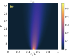
(a)

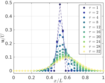
(b)

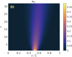
(c)

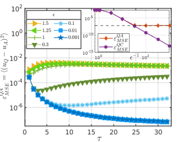
(d)

Figure 3: (a-b) The figure shows contour shaded plots of the evolution of the velocity field as a function of the $x$ direction (with with $N_{g}=32$) and time steps $\tau$ (up to $\tau=32)$. (a) depicts the analytical solution and (b) the quantum solution computed on QFlowS. The system parameters chosen here are: $dt={2.5}\mathrm{e}{-4}$, $D=1$, $\alpha=0.256$, $C=10$ and $\epsilon=0.001$. The color bar indicates the magnitude of the velocity field values. (c) Shows the convergent behavior of the mean-squared-error (MSE) in the quantum solution with respect to the analytical solution. The error is plotted as a function of time for different values of $\epsilon$, using up to a total of 12 qubits. Inset: Taking the MSE at $\tau=32$, we observe that the error when computed with respect to analytical solution (red) begins to saturate for decreasing values of $\epsilon$, while with respect to the classical solution (violet) it continues to decay with a power-law like behavior. Here, the black dotted-line indicates MSE of the classical solution with respect to analytical solution ($\sim{7}\mathrm{e}{-8}$), which clearly forms the lower bound on the MSE of the quantum solutions for small $\epsilon$ and hence explains the observation.

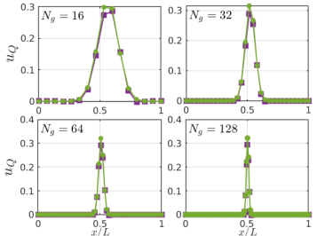
(a)

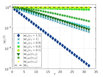
(b)