Receptivity of a supersonic jet due to acoustic excitations near the nozzle lip
Abstract
In this paper, we develop an analytical model to investigate the generation of instability waves triggered by the upstream acoustic forcing near the nozzle lip of a supersonic jet. This represents an important stage, i.e. the jet receptivity, of the screech feedback loop. The upstream acoustic forcing, resulting from the shock-instability interaction, reaches the nozzle lip and excites new shear-layer instability waves. To obtain the newly-excited instability wave, we first determine the scattered sound field due to the upstream forcing using the Wiener-Hopf technique, with the kernel function factored using asymptotic expansions and overlapping approximations. Subsequently, the unsteady Kutta condition is imposed at the nozzle lip, enabling the derivation of the dispersion relation for the newly-excited instability wave. A linear transfer function between the upstream forcing and the newly-excited instability wave is obtained. We calculate the amplitude and phase delay in this receptivity process and examine their variations against the frequency. The phase delay enables us to re-evaluate the phase condition for jet screech and propose a new frequency prediction model. The new model shows improved agreement between the predicted screech frequencies and the experimental data compared to classical models. It is hoped that this model may help in developing a full screech model.
1 Introduction
Screech is a phenomenon characterized by discrete acoustic tones in imperfectly expanded supersonic jet flows (Raman, 1999; Edgington-Mitchell, 2019). Its high intensity can lead to sonic fatigue and severe damage to aircraft structures, emphasizing the importance of understanding its underlying mechanism. In the pioneering work by Powell (1953a), he proposed the well-known feedback-loop mechanism consisting of four stages: the downstream propagation of instability waves, the interaction between shock and instability waves, the upstream propagation of acoustic waves, and the jet receptivity at the nozzle lip. Powell further introduced the gain and phase conditions necessary for establishing the screech. These two conditions laid the foundation of following jet screech research.
The screech frequency, herein defined as , has gained much attention in early research. Powell suggested that it can be calculated by assuming constructive interference at between shock-cell sources, i.e.
| (1) |
where , , and are the shock cell spacing, the convection velocity, and the convective Mach number of the instability waves, respectively. Note, strictly speaking, (1) is not a traditional phase condition in the sense that the overall phase change during the four stages of screech is assumed to be , where is an integer. Nonetheless, the predicted results using (1) demonstrated satisfactory agreement with experimental data regarding rectangular nozzles. Subsequently, Tam et al. (1986) proposed the weakest link theory, suggesting screech as the limit of broadband shock-associated noise (BBSAN) when the observer angle approaches . Based on these two models, new frequency prediction formulas were developed to include effects of nozzle geometry, including rectangular nozzles with different aspect ratios (Tam, 1986; Tam & Reddy, 1996), bevelled rectangular nozzles (Tam et al., 1997), and elliptic nozzle (Tam, 1988). These model predictions exhibited favourable agreement with experimental data.
However, in round jets, Powell observed sudden changes in the screech frequency with increasing inlet pressure, a phenomenon termed mode staging. Powell categorized these changes into four distinct modes: A, B, C, and D, with mode A further divided into modes and (Merle, 1956). It is evident that the aforementioned formulas, which showed continuous frequency predictions against the nozzle inlet pressure, proved inadequate in predicting mode staging. The physical mechanism of mode staging necessitated further investigation.
To investigate the mode staging phenomenon, Li & Gao (2010) introduced the phase condition as an alternative to the constructive interference condition to predict the screech frequency. They conducted comprehensive numerical simulations to thoroughly investigate various parameters regarding the phase condition, including the convection velocity of instability waves, the effective sound source region, and the shock spacing. Their simulation results demonstrated agreement with experimental data when the cycle numbers contained in the feedback loop were changed, suggesting that the phase condition might provide insights into the underlying mechanism of the mode staging phenomenon. Recent years have witnessed a re-evaluation of the phase condition, see for example Jordan et al. (2018) and Mancinelii et al. (2021). These new theories emphasized the crucial role played by the guided-jet mode in completing the feedback loop of jet screech, as evidenced by recent publications (Gojon et al., 2018; Edgington-Mitchell et al., 2018; Li et al., 2020). According to these studies, both the and modes were closed by guided-jet modes rather than free acoustic waves. Moreover, the guided-jet mode was found to be active in all screech modes (Edgington-Mitchell et al., 2022), and its excitation can be attributed to interactions between the instability waves and the optimal order as well as suboptimal wavenumber components of the shock structures (Nogueira et al., 2022; Edgington-Mitchell et al., 2022; Li et al., 2023). The guided-jet mode due to the interaction between instability waves and the suboptimals is shown to be responsible for closing the feedback loop in multiple stages of jet screech. The role of guided-jet modes was also examined under the circumstances of screeching twin jets (Stavropoulos et al., 2023), which showed similar trends to those observed in single jets.
To invoke the phase condition to predict the mode staging phenomenon, an important step is to determine the phase delay between the upstream forcing and the newly-triggered instability waves. This necessitates a close examination of the receptivity process of the jet screech. Previous investigations conducted relevant research using experimental measurements, numerical simulations, and analytical models.
Early research primarily focused on experimental measurements, which revealed that modifications to the nozzle lip, such as nozzle thickening, could change both the mode and amplitude of screech tones (Norum, 1983; Ponton & Seiner, 1992; Raman, 1997). Additionally, an acoustic reflector placed upstream or downstream of the nozzle lip was shown to significantly impact screech amplitude (Nagel et al., 1983; Norum, 1984; Raman et al., 1997). Moreover, it was found that installing conical reflector surfaces around a round nozzle exit could cause significant changes in the mode staging behaviour (Morata & Papamoschou, 2023). Recently, Alapati & Srinivasan (2024) showed that when the surface roughness of the nozzle lip increases, the screech amplitude decreased or even disappeared. These observations underscored the key role played by the jet receptivity in determining the screech amplitude and frequencies.
Besides experimental measurements, several numerical simulations were conducted to investigate jet receptivity. Shen & Tam (2000) explored the effects of nozzle-lip thickness on the intensities of the axisymmetric screech tones. They found that at low supersonic Mach numbers, the changes of the screech amplitude were not significant with a thickened nozzle lip, which aligned with experimental observations (Ponton & Seiner, 1992). Recent years have seen an increase in research on jet receptivity. Karami et al. (2020) defined a transfer function at the nozzle lip between the external disturbance and the initial conditions of the vortical instability in the case of impinging jets. Their findings indicated that the scattering efficiency was related to the nondimensionalized frequency, the azimuthal wavenumber, and the pulse location. Subsequently, Karami & Soria (2021) incorporated the effects of nozzle geometry into their analysis. They noted that an infinite-lipped nozzle supported higher amplitude upstream-propagating waves both inside and outside the jet flow compared to the thin nozzles. Boegy (2022) conducted Large Eddy Simulations (LES) to explore the interaction between upstream-propagating guided jet modes and shear-layer instability waves near the jet nozzle. He observed that the frequency of the most amplified Kelvin-Helmholtz instability wave fell within the narrow frequency bands of the guided-jet mode. The effects of the nozzle thickness were also investigated in Bogey (2023), where it was found that a thickened nozzle lip led to an increase in the near-field sound pressure level downstream of the jet nozzle.
Despite numerous experimental and numerical investigations, not many analytical models were developed to model the jet receptivity. Tam (1978) investigated the excitation of instability waves in infinitely-long two-dimensional free shear layer by acoustic waves, which was solved by using the Green’s function of the problem. He found that to excite instability waves at moderate subsonic flow Mach numbers, an acoustic beam inclined at an angle of to to the shear flow is the most effective. Another notable study conducted by Kerschen (1996) examined the jet receptivity due to acoustic excitations and introduced a receptivity coefficient to predict the screech amplitude. However, comprehensive details of this model appeared missing in the open literature. Another study by Barone & Lele (2005) employed a combined theoretical and computational approach and revealed that upstream-propagating acoustic perturbations could excite instability waves in the jet mixing layer. They further observed that the thickness of the nozzle lip significantly influenced the receptivity process, which accorded with numerous experimental observations.
In spite of numerous studies on jet receptivity, the phase delay in the receptivity process remains unclear. Previous studies often assumed a fixed phase delay such as 0 or (Jordan et al., 2018; Mancinelii et al., 2021; Stavropoulos et al., 2023; Li et al., 2023). To obtain the correct phase delay, instead of relying on assumed values, an analytical model of the jet receptivity is needed. More specifically, a linear transfer function between the upstream forcing and the newly-generated instability wave is desired. Therefore, the primary objective of this paper is to develop such a model to improve our understanding of jet receptivity.
This paper is structured as follows: section 2 provides a detailed analytical derivation of the model, including the formulation of the Wiener-Hopf problem, the decomposition of the kernel function, and the determination of the dispersion relation. A linear transfer function between the upstream forcing and the newly-excited instability waves is obtained. In section 3, we present our results based on the derived transfer function, where a new formula is proposed to predict the screech frequency. Finally, section 4 concludes this paper.
2 Analytical formulation
2.1 The Wiener-Hopf equation
Inspired by Crighton (1992), who investigated jet-edge tones, we focus on a two-dimensional jet flow of a vortex-sheet type in this paper. To render the model more realistic, the incident acoustic wave takes an asymptotic form generated through the interaction between shock and instability waves, as obtained previously by the authors (Li & Lyu, 2022, 2023).
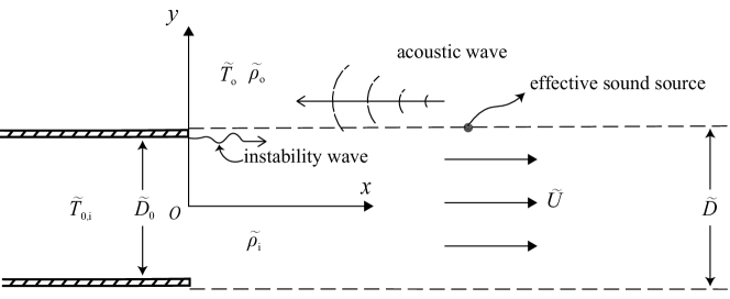
Schematic illustration is shown in figure 1. As we can see, a supersonic jet is issued from the nozzle and takes the form of a vortex sheet. The coordinate axes are chosen to be parallel and perpendicular to the nozzle centreline, respectively, while the origin point is located at the center of the nozzle exit plane. According to Pack (1950), the base flow is chosen as the fully expanded jet velocity , which is different from the jet exit velocity . is the height of the fully expanded jet. Note that is generally not equal to the height of the nozzle (Tam, 1972), but is less or greater than depending on whether the jet is underexpanded or overexpanded (Tam & Tanna, 1982). The densities inside and outside the jet are denoted by and , respectively, while and represent the total reservoir temperature and the ambient temperature outside the jet, respectively. The nozzle lips, represented by two flat plates in figure 1, are assumed to be semi-infinite with a negligible thickness, extending to in the direction. Downstream of the nozzle lip, an acoustic wave, with a speed of sound and a frequency of , is emitted from a source region and propagates upstream to the nozzle lip, triggering the instability waves.
To simplify the problem, we nondimensionalize velocities and lengths by and , respectively. In addition, densities and temperatures are nondimensionalized by and , respectively. Note that we use the symbols with a tilde to represent dimensional variables, while those without denote non-dimensional variables. For example, after the nondimensionalization, the jet exit velocity is and the base flow takes the form
| (2) |
where is the unit vector in the direction.
Considering that the mean pressure outside and inside of the vortex sheet remains the same when a perfect gas is assumed, the density ratio between the outside and inside of the vortex sheet, here defined as , is equal to . Here, and are defined as and , respectively, where and represent the nondimensional speed of sound outside and inside of the jet, respectively. The relation between the two Mach numbers is determined using Crocco-Busemann’s rule, i.e.
| (3) |
where denotes the temperature ratio between and , and represents the specific heat ratio.
Before proceeding to solve the problem, it is useful to examine the designed transfer function using the Buckingham theorem. As mentioned above, eight physical variables are involved in this model, i.e. , , , , , , , and the frequency of the acoustic wave , while four independent dimensions can be found. Employing the Buckingham theorem, it is evident that the transfer function between the newly-excited instability wave and the acoustic waves is related to four nondimensional parameters. These four parameters are chosen to be the Mach number , the Strouhal number , the temperature ratio , and the density ratio . The density ratio can be calculated using and through the Crocco-Busemann’s rule (3). Therefore, there remain three independent nondimensional parameters and our objective is to find the transfer function in the subsequent analysis.
To have a realistic incident acoustic wave, we take the result obtained in the shock-instability interaction work (Li & Lyu, 2022, 2023). Pack’s model was used to describe shock waves, while instability waves were calculated using the linear stability analysis. The resulting nondimensionalized velocity potential function of the acoustic waves due to one-cell interaction can be obtained by performing the inverse Fourier transform, i.e.
| (4) |
Herein denotes the streamwise wavenumber and represents a coefficient, which can be readily calculated when and are provided. The detailed expression of can be found in Li & Lyu (2023). The integration in (4) can be estimated (in the far field) by the saddle point method. The closed-form asymptotic potential function can be expressed as follows
| (5) |
where is the observer angle with respect to the downstream direction and represents the distance from the screech source region to the nozzle lip.
As shown in (5), depends on . Experimental observations indicated that the screech source was situated several shock cells downstream from the nozzle exit (Suda et al., 1993; Kaji & Nishijima, 1996; Malla & Gutmark, 2017). Therefore, the streamwise distance between the source position to the nozzle lip is written as
| (6) |
where typically takes the value of 3, 4, or 5 (Suda et al., 1993; Li & Gao, 2010; Malla & Gutmark, 2017), and denotes the shock spacing, which can be calculated using Pack’s model (Pack, 1950; Tam, 1986).
We consider the potential function of the upstream forcing in the proximity of the nozzle lip, where the value of is relatively small compared to . Therefore, the distance in (5) can be approximated as . Similarly, we have and . Consequently, in the vicinity of the nozzle, the potential function can be reformulated to a similar form to that in Crighton (1992), i.e.
| (7) |
where
| (8) |
| (9) |
The goal is therefore to find the response of the jet flow due to the upstream forcing near the nozzle lip. In this paper, we focus on the upper half-plane (), while a similar analysis can be carried out for the lower half-plane. Considering that the time-harmonic assumption is used, the factor in all the time-dependent fields is omitted for clarity in the rest of this paper. Because we assume the initial base flow to be irrotational and inviscid both inside and outside of the vortex sheet (Batchelor & Gill, 1962), the velocity potential induced by the incident acoustic wave near the nozzle lip can be described by a potential function. Therefore, taking into account (7), the total velocity potentials outside and inside the jet flow can be defined by
| (10) |
| (11) |
respectively, where and are the corresponding potential functions of the scattered sound fields in the region and , respectively.
It is known that and both satisfy the convective wave equation, i.e.
| (12) |
| (13) |
Hard-wall conditions are imposed on for . Note that, strictly speaking, these conditions should be applied at , which can be either less than or greater than depending on whether the jet is underexpanded or overexpanded (Tam & Tanna, 1982). However, as mentioned earlier, the difference between and is relatively small compared to the distance . To enable analysis progress, we neglect this difference and assume that the plate is nearly parallel to the boundary of the jet. Therefore, we obtain
| (14) |
The absence of decay in the forcing term leads to convergence issues when the Fourier transform is applied to (2.13). To circumvent this problem, Crighton (1992) replaced (14) by
| (15) |
where is a real and positive term, which retains the physical characteristics of the upstream forcing near the nozzle lip but removes the forcing further upstream. We follow the same treatment here.
The kinematic and dynamic boundary conditions can be used on the vortex sheet at , i.e.
| (16) |
| (17) |
Fourier transforms are defined by
| (18) | |||
| (19) |
where is the wavenumber in the streamwise direction. Multiplying (12) and (13) with and subsequently integrating both expressions with respect to the variable , solutions to (12) and (13) can be found upon invoking the far-field boundary condition, i.e.
| (20) |
| (21) |
where
| (22) |
Herein, , , and are functions of , whose detailed forms will be specified subsequently. To satisfy the far-field condition, the real part of should be positive, and its branch cut will be specified later. It is well-known that both symmetric (varicose) and antisymmetric (sinuous) instability modes can exist inside the jet. But for jet flows from high-aspect-ratio rectangular nozzles, the sinuous mode is dominant (Edgington-Mitchell, 2019). Therefore, we consider the antisymmetric mode in this study, while the symmetric mode can be examined in a similar way should interest arise. In this case, reduces to
| (23) |
In what follows, we use the Wiener-Hopf method to solve this boundary-value problem specified by (20), (23) and boundary conditions (15), (16), and (17). Using (15), we can obtain
| (24) |
where the prime represents the first derivative with respect to and is defined by
| (25) |
Considering the kinematic boundary condition across the vortex sheet, i.e. (16), and the boundary conditions imposed on the nozzle lip, i.e. (15), we have
| (26) |
Following Crighton (1992), the term on the left-hand side of (26) is omitted, considering that is a small term.
Now we define a new function related to the difference between the pressures outside and inside the vortex sheet as , i.e.
| (27) |
Due to the continuity of the pressure across the vortex sheet, i.e. (17), the pressure difference vanishes when . Therefore, reduces to
| (28) |
where
| (29) |
and denotes the finite value of at the position . Substituting (20) and (23) into (28), we obtain
| (30) |
Combining (24), (26), (28), and (30) yields
| (31) |
where
| (32) |
| (33) |
Equation (31) represents the Wiener-Hopf equation we aim to solve, with the kernel given by . represents the dispersion relation of the antisymmetric mode of the jet instability wave. It can be seen that as , . Now, following the procedures of the Wiener-Hopf method, we assume that the kernel can be decomposed into
| (34) |
where and are analytic and non-zero in the upper and lower half-planes of , respectively. Meanwhile, both and behave as as approaches infinity. The actual decomposition will be shown in section 2.2. Routine use of Wiener-Hopf decomposition leads to
| (35) |
| (36) |
Here is an entire function of . Due to the Kutta condition (Crighton, 1985), behaves like near the nozzle lip. The corresponding value of is therefore . It follows that as (Erfelyi, 1958). Thus, from Liouville’s theorem,
| (37) |
From (24) and (35), can be readily solved, i.e.
| (38) |
It can be seen that is as approaches infinity in the upper half plane. The corresponding velocity component behaves as when , which leads to singularity in due to (16). Therefore, (38) leads to singular behaviour when , where (2.37) can be approximated by (Crighton, 1992)
| (39) |
This part will be further discussed in section 2.3, where the unsteady Kutta condition is used to determine the new instability wave by removing the emerging singularity.
2.2 The kernel decomposition
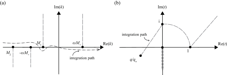
In this section, we factor the kernel into and , which is the essential step of the Wiener-Hopf technique. Before proceeding with the decomposition of the kernel, it is necessary to properly define the branch cuts of . In order to ensure that the real part of is positive as along the integration path (which becomes relevant when conducting the inverse Fourier transform if we are interested in calculating the scattered sound field), the branch cuts of passing the branch points are chosen to extend to the upper and lower half-plane, respectively, as shown in figure 2(a). The branch is selected in such a way that at . On the other hand, the branch points of are determined as and . The branch cuts passing and are chosen to extend to the lower and upper half-plane, respectively, for the convenience of the kernel decomposition. The branch of is selected to ensure that at . Due to the choice of the branch cuts, we can find that , as and .
The kernel can be rewritten as
| (40) |
A proper decomposition of is evident, i.e. . Thus, in what follows we only focus on the denominator, which we refer to as . It can be seen that depends on the dispersion relation of the antisymmetric mode of the jet instability wave. This dispersion relation describes several types of waves present in the jet, determined by its structural characteristics such as branches, zeros, and poles. These information can be maintained if the kernel is decomposed by means of matched asymptotic expansions (Crighton, 1992, 2001). To use this strategy, a small parameter should be specified as the basis for the expansion. This parameter should not only be small but can also be contained by the kernel. We introduce as this parameter. In what follows, the complicated kernel is replaced by a simpler one by asymptotic expansions based on . Overlapping approximations are subsequently applied to guarantee the validity of the decomposition over the whole range of the wavenumber . The final result is obtained by a multiplicative composite approximation.
We first assume and let . The first term of , i.e. reduces to and can be approximated as
| (41) |
The term is supposed to maintain the branch cut chosen for . For brevity, we rewrite as , where the script ∗ represents that this parameter retains the specified branch cuts.
Now, we introduce the small parameter and a new scaled wavenumber according to
| (42) |
By assuming and , we can expand in (2.39) based on the small parameter (using methods of Taylor expansion), i.e.
| (43) |
where . Note that despite the small parameter , the quantities . To put this into perspective, let us consider an example with . At the screech frequency, employing Powell’s original model yields . However, , which is of the order of unity. The scale separation can be shown more clearly as increases. This demonstrates that although itself may be small, its corresponding fractional power can still have magnitudes of the order of unity in our interested application.
We can show that (41) and (43) do overlap, as and , respectively, with common value . A multiplicative composite approximation then reads
| (44) |
where
| (45) |
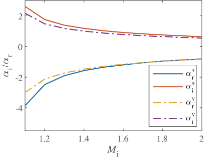
To validate the decomposition, the wavenumber obtained by letting in (44) equal to 0, which corresponds to the wavenumber of the sinuous mode of the jet instability wave, is compared to that numerically solved by the dispersion relation . As shown in figure 3, the agreement between the two wavenumbers is good when . Therefore, in the subsequent analysis, our focus will be in the range of .
We are now in a position to factor the function . From Noble (1956), can be decomposed to
| (46) |
where
| (47) |
Here represents the Gamma function. The decomposition of reads
| (48) |
where
| (49) |
Naturally, the branch cut of and is from to and from to , respectively.
The decomposition of , on the other hand, is very difficult due to the presence of in (45). To decompose , we let be real first (Crighton, 1992), so that . This is reasonable considering that the overlap of the two half-planes will converge to the real axis in the complex plane. Assuming that can be decomposed to , and taking the first derivative of , we obtain
| (50) |
where
Multiplying the numerator and the denominator of the right-hand side term in (50) by , equation (50) can be written as
| (51) |
The zeros of the denominator are defined as , which can be obtained by Ferrari’s formula. The details are provided in Appendix A. With the knowledge of these zeros, we can now reorganize (51) as
| (52) | ||||
where
| (53) |
The detailed derivation from (51) to (52) can be found in Appendix B. For brevity, we can define and . With these definitions, it is straightforward to find
| (54) |
An addictive decomposition of is now introduced, i.e.
| (55) |
where
| (56) |
The branch cuts of and extend from to and from to , respectively. The choice of the branch cut leads to
| (57) |
Using the addictive decomposition (55) and the two identities (54) and (57), the right-hand side of (52) can obtain a similar addictive factorization, and can be finally found as
| (58) |
The detailed derivation from (52) to (58) can be found in Appendix B.
To evaluate the integral in (58), as shown in figure 2(b), we deform the integration path in (58) from to the point , then along a unit circle to reach situated on the real axis, and finally along a ray from to . Using the identity (54), we can evaluate (58) to obtain
| (59) |
Here represents the polylogarithm function of the second order (Gradshteyn & Ryzhik, 1980).
2.3 Instability waves excited by the acoustic waves at the nozzle lip
Under the excitation of the acoustic wave, new instability waves would emerge near the nozzle lip (Crighton, 1985). We can determine this instability wave by imposing the unsteady Kutta condition at the nozzle lip (Crighton, 1981). Following Crighton (1972) and considering that we focus on the upper half-plane (), we assume that the excited instability wave can be represented by
| (63) |
where represents the amplitude of the instability wave and is defined by . The parameter denotes the wavenumber of the instability waves of the antisymmetric mode, and its determination is outlined in Appendix A. The choice of the form in (63) is believed to be reasonable, particularly considering the sinuous nature exhibited by both the upstream forcing and the scattered acoustic field.
The instability wave then propagates downstream and subsequently interacts with the shock structures (Powell, 1953b; Suda et al., 1993; Edgington-Mitchell et al., 2021). This interaction leads to the emission of sound, which serves as the upstream forcing and completes the screech feedback loop. To determine the instability amplitude in (63), we first calculate the scattered field resulting from the newly-excited instability wave at the nozzle lip. The singular component within the resulting scattered field needs to be eliminated using the singularity in (39). This process fixes the value of in order to satisfy the unsteady Kutta condition.
Replacing the forcing term in (10) and (11) with while following the same procedures outlined in section 2.1, we obtain the scattered field due to the presence of the instability wave, i.e.
| (64) |
The component of similar to (39) that leads to singularity is
| (65) |
The unsteady Kutta condition demands no singularity in the vicinity of , therefore from (39) and (65) we must have
| (66) |
The parameter and the kernel function are defined by (8) and (60), respectively. To evaluate , we need to determine the small parameter , which seems to be an arbitrary value introduced to address the issue of non-convergence. However, in fact has a physic-imposed value and we may uniquely determine it by re-evaluating the problem without approximations.
First, replace the forcing term in (10) and (11) by
| (67) |
Then the Wiener-Hopf equation (31) takes a new form, i.e.
| (68) |
Here
| (69) |
where , and the form of is shown in Appendix B. If we intend to completely account for the effect of the upstream forcing, we can replace by and by , and then carry out the integration from to . The mathematical proof of this procedure can be found in Appendix C. Thus, it follows that
| (70) |

The integration on the right-hand side of (70) can be evaluated using Watson’s Lemma. On the left-hand side of (70), given that is a small term, can be evaluated employing its Taylor expansion. By combining (62) and (102), we have
| (71) |
To verify that is a small term, we calculate it using (71) and plot it in figure 4. The angular frequency of the instability wave is calculated using the original formula (1.1) proposed by Powell (1953a). Figure 4 shows that within the range of , the value of initially decreases from its maximal value of at to at , and then gradually increases to around at . In the entire Mach number region, is small, ensuring the validity of using Taylor expansion in (62) and the omission of in (26).
Having obtained all the parameters, the instability wave is found to be
| (72) |
This equation enables us to define the important transfer function, i.e.
| (73) |
where is given by (60), by (91), , and by (71). This transfer function describes the linear mapping between the newly-excited instability waves and the upstream propagating acoustic waves. Using this function, both the scattering efficiency and the phase delay between these two waves can be readily examined.
3 Results
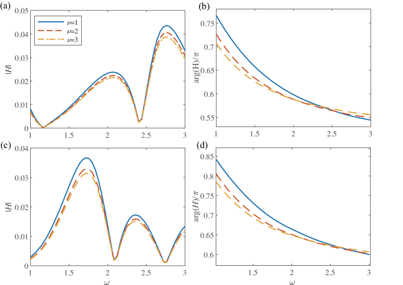
We first investigate the behaviour of the transfer function under two typical screech conditions, i.e. and . We also consider the effects of the temperature by showing results at three temperature ratios, i.e. , 2, and 3. The amplitude, i.e. the scattering efficiency, and the phase of are shown in figure 5. Note that the phase is defined in the range . Considering that the asymptotic expansion yields favourable approximation when , which corresponds to screech frequency within the range of , only the frequency range from 1 to 3 is examined. Figures 5(a) and 5(c) show that the scattering efficiency displays multiple peaks and valleys as the frequency varies. In both cases, is less than and decreases to at certain frequencies. Note that the temperature has a mild impact on the scattering efficiency. Specifically, as the temperature ratio increases, the scattering efficiency decreases slightly. Regarding the phase delay, figures 5(b) and 5(d) show a phase delay between around to , which demonstrates a decreasing trend as the frequency increases. In addition, higher jet temperatures lead to lower phase delays at low frequencies while resulting in slightly higher phase delays at high frequencies.
3.1 Phase condition for jet screech
Using the transfer function, we can examine the phase condition for the screech feedback loop in this section. In the subsequent analysis, we first focus on the cold jet, which corresponds to the operation conditions commonly employed in experiments and numerical simulations. We then incorporate the thermal influence to account for temperature effects on the screech frequency.
The original phase condition proposed by Powell (1953a) can be written as
| (74) |
where and represent the nondimensional phase velocity of the downstream-propagating instability waves and the upstream-propagating acoustic waves, respectively. Note that in this study. The integer denotes the total number of phase cycles contained in the feedback loop, and represents a number between 0 and 1 due to the additional phase delay. Note that this phase criterion can be reformulated, as demonstrated by Jordan et al. (2018) and Mancinelii et al. (2021), in the following manner, i.e.
| (75) |
where and are, respectively, the real part of the wavenumber of the downstream-propagating instability waves and the upstream-propagating acoustic waves. The term is defined as and represents the additional phase delay. As illustrated in figure 6(a), the instability wave with the wavenumber grows spatially from the nozzle lip to the effective source location and interacts with the shock structure. This interaction produces acoustic waves, which propagate to the upstream direction with the wavenumber and trigger new instability waves at the nozzle lip. The total phase variations during this feedback loop must be equal to an integer multiplied by . Therefore, the phase condition can be written as (75). As illustrated in figure 6(a), the total phase delay consists of two components: the phase change occurring during the sound emission () and that during the jet receptivity ().
To predict the screech frequency, the parameters contained in (75), such as , , and should be specified, respectively. Regarding , it is commonly assumed that the phase velocity of the jet instability waves is proportional to the velocity of the fully expanded jet flow. Therefore, we can write as
| (76) |
where typically falls within the range of to , and its value depends on factors such as the nozzle shape and the jet Mach number. In circular nozzles, a value of may be used (Harper-Bourne & Fisher, 1973). However, studies by Li & Gao (2010) have indicated that may vary with the jet Mach number. In the case of a rectangular jet, experiments suggested that values between and may be more appropriate compared to (Powell, 1953a; Krothapalli et al., 1986; Raman & Rice, 1994; Panda et al., 1997). Similarly, variations in due to changes in jet Mach numbers have also been reported (Powell, 1953a; Panda et al., 1997).
Based on experimental measurements and data analysis, Tam & Reddy (1996) proposed an empirical formula to estimate for rectangular nozzles, i.e.
| (77) |
where is the aspect ratio of the rectangular nozzle. For a high-aspect-ratio rectangular jet, Tam & Reddy (1996) and Berland et al. (2007) applied the value of . In the rest of this paper, if no specific data is available, we use this empirical formula to determine .
For , it is straightforward to find that
| (78) |
Combining (6), (75), (76), and (78) yields
| (79) |
Note that, the additional phase delay is typically assumed to be in previous studies (Jordan et al., 2018; Li et al., 2023). The integer , according to the findings of Mercier et al. (2017), is often equal to the shock cell number for circular nozzles. We assume that this relation holds for the two-dimensional jet under consideration. By setting and , equation (79) can be simplified to (1), which represents the original frequency prediction model proposed by Powell (1953a). Note that (1) is derived under the assumption that the sound intensity in the upstream direction reaches its maximum, thus corresponding to the constructive interference condition. We can see that the frequency prediction formula obtained from the phase condition coincides with (1) when and .
As we can see from figure 6(a), an effective screech source is assumed in early research on the phase condition. However, whether the screech source is distributed or localized is still open to debate. As illustrated in figure 6(b), in our previous study (Li & Lyu, 2023), the acoustic wave is generated by the interaction between the instability wave and the distributed shock cells. Consequently, the sound source is distributed across various shock structures, e.g. the fourth and fifth shock structures. Therefore, we cannot pinpoint a specific point source. Nevertheless, without an effective source location, we can still establish a phase condition in this model, i.e.
| (80) |
Here, denotes the distance between the nozzle lip and the left boundary of the source region as shown in figure 6(b). represents the phase of the resulting acoustic wave at the nozzle lip, which is generated from the interaction between the shock structures and an instability wave whose phase is set to be 0 at the left boundary of the source region. The actual phase of the acoustic wave at the nozzle lip, after taking account of the phase variation due to instability propagation, would be , as shown in figure 6(b). denotes the phase change during the jet receptivity, which is the same as that defined in figure 6(a). Similar to (75), the total phase variations during the feedback loop should be equal to an integer multiplied by . Therefore, we can write the phase condition as (80), where a new integer is introduced. We expect because the actual phase variation between the left boundary of the source region and the nozzle lip is probably more than . However, only is included, which is less than under several operation conditions. We find that is often appropriate. From (76) and (80), we can obtain
| (81) |
Equipped with obtained from the transfer function and obtained from Li & Lyu (2023), we can compare this model prediction with Powell’s model prediction and the experimental measurements.
| Cases | ||||||
| Powell (1953a) | 0.6 | 5.83 | 1 | 1 | 4 | 3 |
| Raman & Rice (1994) | 0.54 | 9.63 | 1 | 1.42 | 4 | 3 |
| Panda et al. (1997) | 0.65 | 5 | 1 | 1 | 4 | 3 |
| Alkislar et al. (2003) | 0.63 | 4 | 1.44 | 1 | 4 | 3 |
The operation conditions used in four experiments in the open literature, including the aspect ratio of the rectangular nozzle (), the designed Mach number of the nozzle (), and the temperature ratio () are listed in table 1. In these experiments, the convection velocities of the instability wave were all measured. The constants obtained from these experiments are listed in table 1. Note that in Panda et al. (1997), the constant was found to increase as increased, from 0.6 at low to 0.7 at high . We use an average value of to initiate the computation. In addition, the screech source region was reported to be around the fourth shock structure from experimental observations, thus we set and in the four cases. To calculate the shock spacing in (79) and (81), we use the model proposed by Tam (1988), where can be expressed by
| (82) |
Here represent the nondimensional height and width of the fully expanded jet flow. is related to the jet aspect ratio (), the Mach number of the fully expanded jet flow (), and the designed Mach number (). The method to calculate can be found in Tam (1986).
The phase and the phase delay can be readily calculated if is provided. However, depends on and via (81). So to determine and in (81), we use an iterative scheme as follows. We first employ the operation conditions presented in table 1 and calculate the screech frequency using Powell’s original formula (1). Subsequently, the obtained frequency is substituted into this model to determine and . A new screech frequency can then be predicted using (81). This new frequency can be used to obtain an updated and . The procedures are repeated until a converged frequency is obtained. We first show the phase changes in figure 7. As can be seen, both and increase as the jet Mach number increases. increases in a nearly linear manner with respect to , while varies slowly as changes, increasing from nearly at low Mach numbers to as increases to 1.8.
Equipped with the and , we can calculate from (81). Comparison between this model prediction, Powell’s model prediction, and the experimental data are shown in figure 8. It can be seen that this model predictions agree well with the experimental data in figures 8(c)-(d), while Powell’s model predictions seem to show an overprediction compared to the experiments. Note that in figure 8(c), setting can lead to favourable agreement between Powell’s model prediction and the experimental data, as shown by Berland et al. (2007), whereas using the convection velocity directly obtained from the experimental data leads to an overprediction. In figure 8(a), on the other hand, this model underpredicts the screech frequency, while Powell’s model prediction agrees well with the experimental data. Note, however, if the constant is assumed to be , Powell’s model overpredicts the screech frequency compared with the experimental data, as shown by Tam (1988), while this model prediction would show good agreement with the experimental data. Whether this underprediction is due to an inaccurate is not yet clear and therefore requires further scrutiny. In figure 8(b), both of the two models provide favourable results. Specifically, Powell’s model prediction agrees well with the experimental data when , while this model prediction agrees well with the experimental data at low Mach numbers and high Mach numbers. Generally speaking, the model prediction demonstrates favourable agreement with the experimental data (Raman & Rice, 1994; Panda et al., 1997; Alkislar et al., 2003), suggesting that considering the additional phase delay may rectify the overprediction of the classical model.
In the final part of this section, we consider the thermal influence on the phase condition, which can be accounted for in two ways. Tranditional model of the thermal effect is through the modification of , as shown by (3). This effect was previously considered by Tam et al. (1986) for circular jet flow. They found that under different temperature ratios, the screech frequency can be predicted by
| (83) |
In the rectangular jet flows, a similar formula may be obtained from (79) and (82), assuming , , and , i.e.
| (84) |
| Cases | ||||||
|---|---|---|---|---|---|---|
| 1 | 0.8 | 2 | 1.5 | 1 | 4 | 3 |
| 2 | 0.73 | 2 | 1.5 | 2 | 4 | 3 |
| 3 | 0.64 | 2 | 1.5 | 3 | 4 | 3 |
Note that the difference between (83) and (84) arises from the distinct values of the shock spacing in circular and rectangular jet flows, which can be predicted by Pack’s model (Pack, 1950; Tam, 1988), i.e. for circular nozzles while for rectangular cases.
In this model, from figure 5, we can see that the phase delay is also changed by the temperature ratios. Therefore, to predict the screech frequency more accurately, the changes in the phase delay and the convection velocity should be both accounted for. To quantitatively evaluate the thermal effects, we take three temperature ratios, i.e. , , and into consideration. We calculate the transfer function at the screeching frequency under the three temperature ratios, the phase delays of which are shown in figure 9. Note that the screech frequency is calculated via (1) with the constant . We can see that under the three temperature ratios phase delays increase as the jet Mach number increases. In addition, higher jet temperatures lead to larger phase delays () across the entire range of Mach numbers, which will, according to (81), result in a lower frequency prediction. Note that this appears to contradict figure 5, but this apparent contradiction results from the fact that we are considering the phase delay at the screech frequency for each and , whereas figure 5 considers the phase delay for a given at the same frequency.
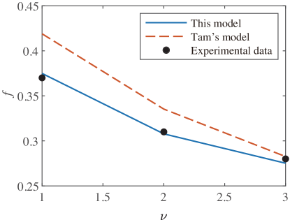
To quantitatively validate (81), we use the data from Gojon et al. (2019), where overexpanded jet flows under different temperature conditions were simulated using LES. The convection velocity of the instability waves was numerically obtained. They compared the frequency prediction from Tam’s model (Tam, 1988) to the reported experimental results (Mora et al., 2016). “An overestimation of about ” (Gojon et al., 2019) compared to the experimental data was reported. This overprediction may be rectified if the calculated is considered. To obtain the screech frequency prediction, we employ the data of the convection velocity from Gojon et al. (2019) and evaluate (81) under the three different temperature ratios. The operation conditions are the same as those used in Gojon et al. (2019) and are listed in table 2. The comparison is shown in figure 10. These results indicate that if the additional phase delay is included, the predicted screech frequency agrees much better with the numerical simulation. Specifically, the overprediction from the classical model is rectified when the phase delay is considered.
4 Conclusion
This paper investigates the jet receptivity occurring at the nozzle lip within the screech feedback loop. The scattered field due to the upstream-propagating acoustic waves is derived using the Wiener-Hopf method, with the kernel decomposed through matched asymptotic expansions. To determine the newly-triggered instability wave, we impose the unsteady kutta condition by eliminating the emerging singularities in the scattered field. This results in a dispersion relation that governs the newly-excited instability waves. The transfer function between the newly-excited instability waves and the upstream forcing is subsequently obtained. The amplitude and phase of the transfer function are then discussed in detail.
The result shows that the scattering efficiency displays multiple peaks and valleys as the frequency increases. In addition, it is less than under each operation condition that we consider. Moreover, the phase delay between the instability wave and the upstream forcing generally decreases as the frequency increases. Regarding the thermal influence on the transfer function, it is found that the scattering efficiency decreases slightly as the temperature ratio increases from 1 to 3, while higher jet temperatures can lead to lower phase delays at low frequencies but result in slightly higher phase delays at high frequencies.
Including this additional phase delay, we invoke the phase condition to predict the screech frequency. The new prediction demonstrates favourable agreement with the experimental data for cold supersonic jets. In particular, the overprediction of screech frequencies from classical models appears to be rectified using the present model, except for the case of Powell’s measurement. In addition, we examine the effects of the temperature ratio on the screech frequency by including the additional phase delay, the result of which shows that the screech frequency prediction improves significantly.
Our future work would focus on the scattering efficiency obtained by the transfer function, which is not thoroughly investigated in this paper due to a lack of direct validation from experimental or numerical data in the open literature. Moreover, the frequency range under consideration is relatively small due to the requirement of the matched asymptotic expansions. We consider to use new strategies to overcome the limitations in our future study.
Appendix A
Following the procedure of Ferrari’s formula, zeros of the polynomial can be determined. Define a parameter as
| (85) |
where
| (86) | |||
| (87) |
The zeros take the following forms, i.e.
| (88) |
| (89) |
Zeros take similar forms, i.e.
| (90) |
| (91) |
where
| (92) |
| (93) |
It can be shown, by some algebra, that when the angular frequency and , and . In addition, can be shown to be a real number.
With a negative real part and a positive imaginary part, ( is defined in section 2.2) corresponds to the wavenumber of the jet instability of the sinuous mode, which is defined as in (63). The original polynomial has four zeros denoted as (in the right half-plane ) and (in the left half-plane ). The additional zeros are due to the increase in the polynomial order.
To further validate the decomposition, we present the additional comparison between the wavenumber numerically obtained by the dispersion relation and that calculated through the asymptotic expansions using different temperature ratios. We see that for the heated jets under consideration ( or ) the agreement between the two wavenumbers remains satisfactory as .
Appendix B
We first provide the detailed derivation from (51) to (52). Substracting the left-hand side and right-hand side of (51) with , the left-hand side part can be directly written as
Using partial fraction decomposition, we can assume that the right-hand side part takes the following form, i.e.
| (94) |
where . The undetermined coefficient can be calculated by multiplying the left-hand and right-hand side of (94) with the corresponding and letting subsequently.
In what follows, we provide the detailed derivation from (52) to (58). Using the addictive decomposition (55) and the identity (54), the right-hand side of (52) can be rewritten as
| (95) |
which can be reorganized as
| (96) |
Using the identity (57), we can reduce (96) to
Considering that and should be analytic and non-zero in the upper and lower half-planes respectively, we can properly write as the form shown in (58).
Appendix C
To calculate the acoustic wave propagating just outside the jet flow, i.e. , it is convenient to deform the integration path in (4) along the branch cut of at . In this way, the difference in the value of on two different sides of the branch cut only comes from . can be thus expressed as
| (97) |
where , and . It is straightforward to see that only contains (the definition of can be found in Li & Lyu (2023)). We can define a new function as follows:
| (98) |
can be then reorganized as
| (99) |
where
| (100) |
Letting and performing a coordinate transformation from to , we can write the function in (69) as
| (101) |
It can be proved that as , takes the following asymptotic forms, i.e.
| (102) |
Here, is what we aim to find to determine in (71), which can be calculateed by letting in (101), while , a coefficient of order , is not presented here for clarity.
In what follows, we provide a proof of the relation (70), which is essential to uniquely determine . The approximated form of the upstream forcing can be written as
| (103) |
while without an approximation, the forcing reads
| (104) |
These two expressions should be virtually the same when . Multiplying (103) and (104) with and integrating each expression with respect to from to , we can find that (103) and (104) can be respectively evaluated as
| (105) |
Subsequently, integrating each expression with respect to from to yields (70).
Acknowledgments
The first author B. Li gratefully acknowledge Y. Ye for his helpful advice on numerical integration. The authors wish to gratefully acknowledge the financial support from Laoshan Laboratory under the grant number of LSKJ202202000.
References
- Alapati & Srinivasan (2024) Alapati, J. K. K. & Srinivasan, K. 2024 Screech receptivity control using exit lip surface roughness for under-expanded jet noise reduction. Physics. Fluids 36(1), 016113.
- Alkislar et al. (2003) Alkislar, M. B., Krothapalli, A. & Lourenco, L. M. 2003 Structure of a screeching rectangular jet: a stereoscopic particle image velocimetry study. J. Fluid Mech. 489, 121–154.
- Barone & Lele (2005) Barone, M. F. & Lele, S. K. 2005 Receptivity of the compressible mixing layer. J. Fluid Mech. 540, 301–335.
- Batchelor & Gill (1962) Batchelor, G. K. & Gill, A. E. 1962 Analysis of the stability of axisymmetric jets. J. Fluid Mech. 14(4), 529–551.
- Berland et al. (2007) Berland, J., Bogey, C. & Bailly, C. 2007 Numerical study of screech generation in a planar supersonic jet. Phys. Fluids 19(7), 075105.
- Boegy (2022) Boegy, C. 2022 Interactions between upstream-propagating guided jet waves and shear-layer instability waves near the nozzle of subsonic and nearly ideally expanded supersonic free jets with laminar boundary layers. J. Fluid Mech. 949, A41.
- Bogey (2023) Bogey, C. 2023 Effects of nozzle-lip thickness on the tones in the near-field pressure spectra of high-speed jets. In AIAA Aviation 2023 Forum. AIAA Paper 2023-3935.
- Crighton (1972) Crighton, D. G. 1972 The excess noise field of subsonic jets. J. Fluid Mech. 56(4), 683–694.
- Crighton (1981) Crighton, D. G. 1981 Acoustics as a branch of fluid mechanics. J. Fluid Mech. 106, 261–298.
- Crighton (1985) Crighton, D. G. 1985 The kutta condition in unsteady flow. Annu. Rev. Fluid Mech. 17(1), 411–445.
- Crighton (1992) Crighton, D. G. 1992 The jet edge-tone feedback cycle: linear theory for the operating stages. J. Fluid Mech. 234, 361–391.
- Crighton (2001) Crighton, D. G. 2001 Asymptotic factorization of wiener–hopf kernels. Wave Motion 33(1), 51–65.
- Edgington-Mitchell (2019) Edgington-Mitchell, D. 2019 Aeroacoustic resonance and self-excitation in screeching and impinging supersonic jets – a review. Int. J. Aeroacoust 18(2-3), 118–188.
- Edgington-Mitchell et al. (2018) Edgington-Mitchell, D., Jaunet, V., Jordan, P., Towne, A., Soria, J. & Hinnery, D. 2018 Upstream-travelling acoustic jet modes as a closure mechanism for screech. J. Fluid Mech. 855, R1.
- Edgington-Mitchell et al. (2022) Edgington-Mitchell, D., Li, X., Liu, N., He, F., Wong, T. Y., Mackenzie, J. & Nogueira, P. 2022 A unifying thoery of jet screech. J. Fluid Mech. 945, A8.
- Edgington-Mitchell et al. (2021) Edgington-Mitchell, D., Wang, T., Nogueira, P., Schmidt, O., Jaunet, V., Duke, D., Jordan, P. & Towne, A. 2021 Waves in screeching jets. J. Fluid Mech. 913, A7.
- Erfelyi (1958) Erfelyi, A. 1958 Asymtotic expansions, 3rd edn., chap. 2. Combridge: Pergamon.
- Gojon et al. (2018) Gojon, R., Bogey, C. & Mihaescu, M. 2018 Oscillation modes in screeching jets. AIAA J. 56(7), 2918–2924.
- Gojon et al. (2019) Gojon, R., Gutmark, E. & Mihaescu, M. 2019 Antisymmetric oscillation modes in rectangular screeching jets. AIAA J. 57(8), 3422–3441.
- Gradshteyn & Ryzhik (1980) Gradshteyn, I. S. & Ryzhik, I. M. 1980 Table of Integrals, Series and Products., 3rd edn. Cambridge: Academic.
- Harper-Bourne & Fisher (1973) Harper-Bourne, M. & Fisher, M. J. 1973 The noise from shock waves in supersonic jets. AGARD Technical Report CP-131 11, 1–13.
- Jordan et al. (2018) Jordan, P., Jaunet, V., Towne, A., Cavalieri, A. V. G., Colonius, T., Schmidt, O. & Agarwal, A. 2018 Jet–flap interaction tones. J. Fluid Mech. 853, 333–358.
- Kaji & Nishijima (1996) Kaji, S. & Nishijima, N. 1996 Pressure field around a rectangular supersonic jet in screech. AIAA J. 34(10), 1990–1996.
- Karami & Soria (2021) Karami, S. & Soria, J. 2021 Influence of nozzle external geometry on wavepackets in under-expanded supersonic impinging jets. J. Fluid Mech. 929, A20.
- Karami et al. (2020) Karami, S., Stegeman, P. C., Ooi, A., Theofilis, V. & Soria, J. 2020 Receptivity characteristics of under-expanded supersonic impinging jets. J. Fluid Mech. 889, A27.
- Kerschen (1996) Kerschen, E. J. 1996 Receptivity of shear layers to acoustic disturbances. In 1st AIAA Theoretical Fluid Mechanics Meeting, AIAA Paper 96-2135.
- Krothapalli et al. (1986) Krothapalli, A., Hsia, Y., Baganoff, D. & Karamecheti, K. 1986 The role of screech tones in mixing of an underexpanded rectangular jet. J. Sound Vib. 106(1), 119–143.
- Li & Lyu (2022) Li, B. & Lyu, B. 2022 Acoustic emission due to the interaction between shock and instability waves in supersonic jet flow from a circular nozzle. In 28th AIAA/CEAS Aeroacoustics 2022 Conference. AIAA Paper 2022-3029.
- Li & Lyu (2023) Li, B. & Lyu, B. 2023 Acoustic emission due to the interaction between shock and instability waves in two-dimensional supersonic jet flows. J. Fluid Mech. 954, A35.
- Li et al. (2023) Li, X., Wu, X., Liu, L., Zhang, X., Hao, P. & He, F. 2023 Acoustic resonance mechanism for axisymmetric screech modes of underexpanded jets impinging on an inclined plate. J. Fluid Mech. 956, A2.
- Li et al. (2020) Li, X., Zhang, X., Hao, P. & He, F. 2020 Acoustic feedback loops for screech tones of underexpanded free round jets at different modes. J. Fluid Mech. 902, 71–96.
- Li & Gao (2010) Li, X. D. & Gao, J. H. 2010 A multi-mode screech frequency prediction formula for circular supersonic jets. J. Acoust. Soc. Am. 127(3), 1251–1257.
- Malla & Gutmark (2017) Malla, B. & Gutmark, E. 2017 Nearfield Characterization of a Low Supersonic Single Expansion Ramp Nozzle with Extended Ramps. In 55th AIAA Aerospace Sciences Meeting. AIAA Paper 2017-0131.
- Mancinelii et al. (2021) Mancinelii, M., Jaunet, V., Jordan, P. & Towne, A. 2021 A complex-valued resonance model for axisymmetric screech tones in supersonic jets. J. Fluid Mech. 928, A32.
- Mercier et al. (2017) Mercier, B., Castelain, T. & Bailly, C. 2017 Experimental characterisation of the screech feedback loop in underexpanded round jets. J. Fluid Mech. 824, 202–229.
- Merle (1956) Merle, M. 1956 Sur la fre’quencies des sondes e’mises par un jet d’air and ‘a grand vitesse. C. R. Academy of Science Paris 243, 490–493.
- Mora et al. (2016) Mora, P., Baier, F., Gutmark, E. J. & Kailasanath, K. 2016 Acoustics from a Rectangular C-D Nozzle Exhausting over a Flat Surface. In 22nd AIAA/CEAS Aerospace Sciences Meeting and Exhibit. AIAA Paper 2016-1884.
- Morata & Papamoschou (2023) Morata, D. & Papamoschou, D. 2023 Influence of nozzle external geometry on the emission of screech tones. Int. J. Aeroacoust 22(5-6), 459–480.
- Nagel et al. (1983) Nagel, R. T., Denham, J. W. & Papathanasiou, A. G. 1983 Supersonic jet screech tone cancellation. AIAA J. 21, 1541–1545.
- Noble (1956) Noble, B. 1956 Methos based on the Wiener-Hopf technique, 3rd edn., p. 41. New York: Nover.
- Nogueira et al. (2022) Nogueira, P. A. S., Jaunet, V., Mancinelli, M., Jordan, P. & Edgington-Mitchell, D. 2022 Closure mechanism of the a1 and a2 modes in jet screech. J. Fluid Mech. 936, A10.
- Norum (1983) Norum, T. D. 1983 Screech suppression in supersonic jets. AIAA J. 21(2), 235–240.
- Norum (1984) Norum, T. D. 1984 Control of jet shock associated noise by a reflector. In 9th Aeroacoustics Conference, AIAA Paper 1984-2279.
- Pack (1950) Pack, D. C. 1950 A note on prandtl’s formula for the wave-length of a supersonic gas jet. Qyart. Journ. Mech. and Applied Math. 3(2), 173–181.
- Panda et al. (1997) Panda, J., Raman, G. & Zaman, K. B. M. Q. 1997 Underexpanded screeching jets from circular, rectangular and elliptic nozzles. In 22nd AIAA/CEAS Aerospace Sciences Meeting and Exhibit. AIAA Paper 97-1623.
- Ponton & Seiner (1992) Ponton, M. & Seiner, J. 1992 The effects of nozzle exit lip thickness on plume resonance. J sound Vib. 154(3), 531–549.
- Powell (1953a) Powell, A. 1953a The noise of choked jets. J. Acoust. Soc. Am. 25(3), 385–389.
- Powell (1953b) Powell, A. 1953b On the noise emanating from a two-dimensional jet above the critical pressure. Aeronautical Quarterly 4(2), 103–122.
- Raman (1997) Raman, G. 1997 Screech tones from rectangular jets with spanwise oblique shock-cell structures. J. Fluid Mech. 330, 141–168.
- Raman (1999) Raman, G. 1999 Supersonic jet screech: Half-century from powell to the present. J. Sound Vib. 225(3), 543–571.
- Raman et al. (1997) Raman, G., Panda, J. & Zaman, K. B. M. Q. 1997 Feedback and receptivity during jet screech: influence of an upstream reflector. In 3rd AIAA/CEAS Aeroacoustics Conference. AIAA Paper 97-0144.
- Raman & Rice (1994) Raman, G. & Rice, E. J. 1994 Instability modes excited by natural screech tones in a supersonic rectangular jet. Phys. Fluids 6(12), 3999–4008.
- Shen & Tam (2000) Shen, H. & Tam, C. K. W. 2000 Effects of jet temperature and nozzle-lip thickness on screech tones. AIAA J. 38(5), 762–767.
- Stavropoulos et al. (2023) Stavropoulos, M. N., Mancinelli, M., Jordan, P., Jaunet, V., Weightman, J., Edgington-Mitchell, D. M. & Nogueira, P. A. S. 2023 The axisymmetric screech tones of round twin jets examined via linear stability theory. J. Fluid Mech. 965, A11.
- Suda et al. (1993) Suda, H., Manning, T. A. & Kaji, S. 1993 Transition of oscillation modes of rectangular supersonic jet in screech. In 15th AIAA Aeroacoustics Conference. AIAA Paper 93-4323.
- Tam (1972) Tam, C. K. W. 1972 On the noise of a nearly ideally expanded supersonic jet. J. FLuid Mech. 51, 69–95.
- Tam (1978) Tam, C. K. W. 1978 Excitation of instability waves in a two-dimensional shear layer by sound. J. Fluid Mech. 89(2), 357–371.
- Tam (1986) Tam, C. K. W. 1986 On the screech tones of supersonic rectangular jets. In 10th Aeroacoustics Conference. AIAA Paper 86-1866.
- Tam (1988) Tam, C. K. W. 1988 The shock-cell structures and screech tone frequencies of rectangular and non-axisymmetric supersonic jets. J. Sound Vib. 121(1), 135–147.
- Tam & Reddy (1996) Tam, C. K. W. & Reddy, N. N. 1996 Prediction method for broadband shock-associated noise from supersonic rectangular jets. J. Aircr. 33(2), 298–303.
- Tam et al. (1986) Tam, C. K. W., Seiner, J. M. & YU, J. C. 1986 Proposed relationship between broadband shock associated noise and screech tones. J. Sound Vib. 110(2), 309–321.
- Tam et al. (1997) Tam, C. K. W., Shen, H. & Raman, G. 1997 Screech tones of supersonic jets from bevelled rectangular nozzles. AIAA J. 35(7), 1119–1125.
- Tam & Tanna (1982) Tam, C. K. W. & Tanna, H. K. 1982 Shock associated noise of supersonic jets from convergent-divergent nozzles. J. Sound Vib. 81(3), 337–358.