Time-Varying Graph Signal Recovery Using High-Order Smoothness and Adaptive Low-rankness

Abstract

Time-varying graph signal recovery has been widely used in many applications, including climate change, environmental hazard monitoring, and epidemic studies. It is crucial to choose appropriate regularizations to describe the characteristics of the underlying signals, such as the smoothness of the signal over the graph domain and the low-rank structure of the spatial-temporal signal modeled in a matrix form. As one of the most popular options, the graph Laplacian is commonly adopted in designing graph regularizations for reconstructing signals defined on a graph from partially observed data. In this work, we propose a time-varying graph signal recovery method based on the high-order Sobolev smoothness and an error-function weighted nuclear norm regularization to enforce the low-rankness. Two efficient algorithms based on the alternating direction method of multipliers and iterative reweighting are proposed, and convergence of one algorithm is shown in detail. We conduct various numerical experiments on synthetic and real-world data sets to demonstrate the proposed method’s effectiveness compared to the state-of-the-art in graph signal recovery.

1 Introduction

Many real-world datasets are represented in the form of graphs, such as sea surface temperatures, Covid-19 cases at regional or global levels, and PM 2.5 levels in the atmosphere. Graphs play a crucial role in data science, facilitating the mathematical modeling of intricate relationships among data points. Typically composed of vertices with either undirected or directed edges, graphs regard each data point as a vertex and use edges to represent pairwise connections in terms of distances or similarities. A graph signal is a collection of values defined on the vertex set. The graph structure can be either provided by specific applications or learned from partial or complete datasets.

As an extension of (discrete) signal processing, graph signal processing shuman2013emerging has become an emerging field in data science and attracted tremendous attention due to its capability of dealing with big data with irregular and complex graph structures from various applications, such as natural language processing mills2013graph , traffic prediction tremblay2014graph , climate change monitoring sandryhaila2013discrete , and epidemic prediction giraldo2020minimization . Graph signal recovery aims to recover a collection of signals with certain smoothness assumptions defined on a graph from partial and/or noisy observations. Unlike signals defined in traditional Euclidean spaces, the intricate geometry of the underlying graph domain must be considered when processing and recovering graph signals. Graph signals typically exhibit smoothness either locally or globally over the graph.

There are some challenges in graph signal recovery when exploiting the underlying graph structure to improve signal reconstruction accuracy. First, the topology of a graph desires a comprehensive representation involving many graph components, such as structural properties, connectivity patterns, vertex/edge density, and distribution. Second, it may be insufficient to describe the smoothness of graph signals by simply restricting the similarity of signal values locally. Moreover, the growth of graph size leads to a significant computational burden. To address them, various techniques have been developed, including graph-based regularization methods chen2015signal ; kroizer2019modeling ; li2023robust ; chen2024manifold , spectral graph theory varma2015spectrum ; domingos2020graph ; ozturk2021optimal ; ying2021spectral , and optimization algorithms berger2017graph ; jiang2020recovery .

1.1 Time-Varying Graph Signal Recovery

A time-varying or spatial-temporal graph signal can be considered as a sequence of signals arranged chronologically, where each signal at a specific time instance is defined on a static or dynamically changing spatial graph.

Consider an undirected unweighted graph $G=(V,E),$ where $V$ is a set of $n$ vertices and $E$ is a set of edges. We assume a collection of time-varying graph signals $\{\mathbf{x}_{t}\}_{t=1,\ldots,m}$ with $\mathbf{x}_{t}\in\mathbb{R}^{n}$ are defined on $V$ with a time index $t$. Let $X=[\mathbf{x}_{1},\ldots,\mathbf{x}_{m}]\in\mathbb{R}^{n\times m}$ be the data set represented in matrix. The pairwise connections on the graph $G$ can be modeled by an adjacency matrix $A$, where the $(i,j)$-th entry of $A$ is one if there is an edge between vertices $i$ and $j$, and zero otherwise. This binary adjacency matrix can be extended to the non-binary case for a weighted graph, where each entry indicates the similarity between two vertices. Throughout the paper, we use a standard $k$ nearest neighbor (kNN) approach based on the Euclidean distance of data points to construct the adjacency matrix.

Given an adjacency matrix $A$, we further define the graph Laplacian matrix, $L=M-A\in\mathbb{R}^{n\times n},$ where $M$ is a diagonal matrix with its diagonal element ${M}_{ii}=\sum_{j}{A}_{ij}$. The graph Laplacian serves as a matrix representation of the graph structure and can be used to describe some important characteristics of a graph, such as node connectivity and similarity. For example, geographic locations in the form of coordinates, i.e., longitude and latitude, are typically used to calculate the pairwise distance and, thereby, the graph Laplacian for geospatial data. For some data sets without obvious graph domains, a preprocessing step of graph learning can be implemented; see xia2021graph for a comprehensive review of graph learning techniques.

Time-varying graph signal recovery aims to recover an underlying matrix from its partially observed entries that are possibly polluted by additive noise. Mathematically, a forward model is $Y=J\circ X+\mathcal{N}$, where $Y$ is the observed data, $J\in\{0,1\}^{n\times m}$ is a sampling matrix, and $\mathcal{N}$ is a random noise. In this work, we focus on recovering time-varying signals, represented by the matrix $X$, from incomplete noisy data $Y$ defined on static spatial graphs in the sense that the vertex set and the edges do not change over time. In addition, we adopt a symmetrically normalized graph Laplacian that is pre-computed based on geographic locations.

1.2 Related Works

The recovery of graph signals from partial observations is an ill-posed problem due to missing data. Graph regularization plays a crucial role in developing a recovery model for time-varying signals by enforcing temporal correlation and/or describing the underlying graph topology. An intuitive approach for recovering time-varying graph signals is to apply interpolation methods to fill in the missing entries, such as natural neighborhood interpolation (NNI) sibson1981brief . Numerous recovery models with diverse smoothness terms have been proposed to further preserve the underlying geometry. For example, Graph Smoothing (GS) narang2013localized characterizes the smoothness of the signal using the graph Laplacian of $X$. Alternatively, temporal smoothness is incorporated in Time-Varying Graph Signal Recovery (TGSR) qiu2017time by formulating the graph Laplacian of $DX,$ where $D$ is a first-order temporal difference operator. The combination of the graph Laplacian of $X$ and the Tikhonov regularity of $DX$ was considered in perraudin2017towards . In contrast, the graph Laplacian of $DX$ with an additional low-rank regularity of $X$ was formulated as Low-Rank Differential Smoothness (LRDS) mao2018spatio . In the Tikhonov regularization, $\left\lVert XD\right\rVert_{F}^{2}=\operatorname*{tr}(XDD^{T}X^{T})$ implies that $DD^{T}$ is treated as the temporal graph Laplacian. In giraldo2022reconstruction , the graph Laplacian matrix $L$ is replaced by $(L+\epsilon I)^{r}$, where $I$ is the identity matrix and $r\geq 1$ for a high-order Sobolev spatial-temporal smoothness. Its main advantage lies in faster convergence, as this approach does not necessitate extensive eigenvalue decomposition or matrix inversion. Recently, another low-rank and graph-time smoothness (LRGTS) method has been proposed in liu2023time , where the sum of the nuclear norm and the Tikhonov regularizer on the second-order temporal smoothness is adopted to promote the low-rankness and the temporal smoothness, respectively.

All the models mentioned above can be condensed into one minimization framework:

$$\min_{X}\leavevmode\nobreak\ \frac{1}{2}\left\lVert Y-J\circ X\right\rVert_{F}^{2}+\frac{\alpha}{2}\operatorname*{tr}(D_{\theta}^{T}X^{T}L_{s}XD_{\theta})+\beta R(X)+\frac{\gamma}{2}\operatorname*{tr}(XL_{t}X^{T}),$$ (1)

where $D_{\theta}$ is a $\theta$-th order temporal difference operator, $L_{s}$ and $L_{r}$ are the spatial and temporal graph Laplacian matrices, respectively, $R(X)$ is the regularization term applied to $X$ describing its characteristics, and $\alpha\geq 0,\leavevmode\nobreak\ \beta\geq 0,\leavevmode\nobreak\ \gamma\geq 0$ are three parameters. Two common choices of $\theta$ are (1) $\theta=0$ that corresponds to $D_{\theta}=I$ and (2) $\theta=1$ used in TGSR. Additionally, $L_{s}$ can be a transformed version of the classical graph Laplacian $L$, e.g., $\tilde{L}=(L+\epsilon I)^{r}$ in the Sobolev method giraldo2022reconstruction , where $\epsilon>0$ and $r\geq 1$, which can be non-integer. The temporal graph Laplacian can be constructed by using the $\tau$-th order temporal difference operator, i.e., $L_{t}=D_{\tau}D_{\tau}^{T}$, for which case the temporal Laplacian can be expressed via the Frobenious norm $\operatorname*{tr}(XD_{\tau}D_{\tau}^{T}X^{T})=\left\lVert XD_{\tau}\right\rVert_{F}^{2}$ (see Tikhonov with $\tau=1$ and LRGTS with $\tau=2$). The regularization $R(X)$ can be chosen as the nuclear norm of $X$ if the underlying time-varying graph signal $X$ is low rank. Various models utilize different choices of $D_{\theta},L_{s}/\tilde{L},L_{t}$, and the regularization $R$. Leveraging the recent growth in deep learning, some time-varying graph signal recovery methods include unrolling technique kojima2023restoration , graph neural network (GNN) castro2023time , and joint sampling and reconstruction of time-varying graph signals xiao2023joint . In this work, we are dedicated to developing unsupervised time-varying graph signal recovery algorithms that do not involve or rely on data training.

Method	Optimization Model
GS narang2013localized	$\min_{X}\frac{1}{2}\left\lVert Y-J\circ X\right\rVert_{F}^{2}+\frac{\alpha}{2}\operatorname*{tr}(X^{T}LX)$ ($\theta=\beta=\gamma=0$ )
Tikhonov perraudin2017towards	${\min_{X}\frac{1}{2}\left\lVert Y-J\circ X\right\rVert_{F}^{2}+\frac{\alpha}{2}\operatorname*{tr}(X^{T}LX)+\frac{\gamma}{2}\left\lVert XD_{1}\right\rVert_{F}^{2}}$ ($\theta=\beta=0,L_{t}=D_{1}D_{1}^{T}$ )
TGSR qiu2017time	$\min_{X}\frac{1}{2}\left\lVert Y-J\circ X\right\rVert_{F}^{2}+\frac{\alpha}{2}\operatorname*{tr}(D_{1}^{T}X^{T}LXD_{1})$ ( $\theta=1,\beta=\gamma=0$)
LRDS mao2018spatio	$\min_{X}\frac{1}{2}\left\lVert Y-J\circ X\right\rVert_{F}^{2}+\frac{\alpha}{2}\operatorname*{tr}(D_{1}^{T}X^{T}LXD_{1})+\beta\|X\|_{*}$    ($\theta=1,\gamma=0$)
Sobolev giraldo2022reconstruction	${\min_{X}\frac{1}{2}\left\lVert Y-J\circ X\right\rVert_{F}^{2}+\frac{\alpha}{2}\operatorname*{tr}(D_{1}^{T}X^{T}(L+\epsilon I)^{r}XD_{1})}$ ($\theta=1,L_{s}=\tilde{L},\beta=\gamma=0$)
LRGTS liu2023time	$\min_{X}\frac{1}{2}\left\lVert Y-J\circ X\right\rVert_{F}^{2}+\frac{\alpha}{2}\operatorname*{tr}(X^{T}LX)+\beta\left\lVert X\right\rVert_{*}+\frac{\gamma}{2}\left\lVert XD_{2}\right\rVert_{F}^{2}$ ($\theta=0,L_{t}=D_{2}D_{2}^{T}$)
Proposed L2	${\min_{X}\frac{1}{2}\left\lVert Y-J\circ X\right\rVert_{F}^{2}+\frac{\alpha}{2}\operatorname*{tr}(D_{\theta}^{T}X^{T}(L+\epsilon I)^{r}XD_{\theta})+\beta\left\lVert X\right\rVert_{\text{erf}}}$ ($\gamma=0$) where $\left\lVert X\right\rVert_{\text{erf}}$ is an ERF weighted nuclear norm
Proposed L1	$\min_{X}\left\lVert Y-J\circ X\right\rVert_{1}+\frac{\alpha}{2}\operatorname*{tr}(D_{\theta}^{T}X^{T}(L+\epsilon I)^{r}XD_{\theta})+\beta\left\lVert X\right\rVert_{\text{erf}}$ ($\gamma=0$) where $\left\lVert X\right\rVert_{\text{erf}}$ is an ERF weighted nuclear norm

Table 1: Comparison of Related Works and Proposed Methods.

Following the general framework (1), we propose a novel low-rank regularization $R(X)$ based on the error function (ERF) guo2021novel for sparse signal recovery (see Section 2.3). In addition, to handle non-Gaussian type of noise such as Laplace noise, we propose a variant model in which the Frobeinus norm based data fidelity term is replaced with the $\ell_{1}$-norm data fidelity (see Section 2.4). In Table 1, we provide a summary of the proposed models and relevant works pertaining to the general framework outlined in (1).

1.3 Contributions

The major contributions of this work are described as follows.

1. We develop a generalized time-varying graph signal recovery framework encompassing several state-of-the-art works as specific cases. We also develop two new models with a new regularization based on ERF.

2. The proposed models combine high-order temporal smoothness and graph structures with the temporal correlation exploited by iteratively reweighted nuclear norm regularization.

3. We propose an efficient algorithm for solving the proposed models. Convergence analysis has shown that the algorithm generates a sequence that converges to a stationary point of the problem.

4. We conduct various numerical experiments, utilizing both synthetic and real-world datasets (specifically PM2.5 and sea surface temperature data), to validate the effectiveness of the proposed algorithm.

1.4 Organization

The subsequent sections of this paper are structured as follows. In Section 2, we introduce a pioneering framework for recovering time-varying graph signals, leveraging Sobolev smoothness and ERF regularization. Additionally, we put forth an efficient algorithm based on the alternating direction method of multipliers (ADMM) and iterative reweighting scheme. A comprehensive convergence analysis of the proposed algorithm is also provided. In Section 3, we present numerical experiments conducted on synthetic and real-world datasets sourced from environmental and epidemic contexts. Finally, Section 4 encapsulates our conclusions and outlines potential avenues for future research.

2 Proposed Method

2.1 Error Function Weighted Nuclear Norm Regularization

To enhance the low-rankness of a matrix, weighted nuclear norm minimization (WNNM) has been developed with promising performance in image denoising gu2014weighted . Specifically, the weighted nuclear norm (WNN) is defined as

$$\left\lVert L\right\rVert_{\mathbf{w},*}:=\sum_{i}w_{i}\sigma_{i}(L),$$ (2)

where $\sigma_{i}(L)$ is the $i$-th singular value of $L$ in the decreasing order and the weight vector $\mathbf{w}=(w_{i})$ is in the non-decreasing order with $w_{i}\geq 0$ being the $i$-th weight. Choosing the weights is challenging in sparse and low-rank signal recovery problems. Iteratively reweighted L1 (IRL1) candes2008enhancing was proposed for the sparse recovery problem, where the weight is updated based on the previous estimate. It can solve many problems with complicated sparse regularizations, exhibiting improved sparsity and convergence speed.

In this work, we introduce a novel ERF-weighted nuclear norm based on the ERF regularizer guo2021novel and use linearization to obtain WNN. For any real matrix $X$ with $n$ singular values $\sigma_{1}(X)\geq\ldots\geq\sigma_{n}(X)$, the ERF-weighted nuclear norm is

$$\left\lVert X\right\rVert_{\operatorname*{erf}}=\sum_{i=1}^{n}\int_{0}^{\sigma_{i}(X)}e^{-t^{2}/\sigma^{2}}dt,$$ (3)

where $\sigma$ serves as a filtering parameter. To solve the ERF-nuclear norm regularized minimization problem, we use iterative reweighting (linearization) to get WNN with adaptive weights.

2.2 Fractional-order derivative

Inspired by the Grünwald-Letnikov fractional derivative podlubny1999fractional , we introduce the total $\theta$-th order temporal forward difference matrix with a zero boundary condition, as shown below

$$D_{\theta}=\begin{bmatrix}C(0)&&&\\ \vdots&\ddots&&&\\ C(k)&\cdots&C(0)&&\\ &\ddots&&\ddots\\ &&C(k)&\cdots&C(0)\end{bmatrix}\in\mathbb{R}^{m\times m}.$$ (4)

Here the coefficients $\{C(i)\}_{i=0}^{k}$ are defined as

$$C(i)=\frac{\Gamma(\theta+1)}{\Gamma(i+1)\Gamma(\theta+1-i)},\quad 0\leq i\leq k,$$

where $\Gamma(x)$ is the Gamma function. Notice that if $\theta$ is a positive integer, $k$ can be deterministic. For example, if $\theta=1$, then $k=1$ and we have $C(0)=1$ and $C(1)=-1$, which is reduced to the first-order finite difference case. If $\theta=2$, then it reduces to the temporal Laplacian operator. Generally if $\theta=n$, then only the first $n+1$ coefficients $\{C(i)\}_{i=0}^{n}$ are nonzero and thereby $k=n+1$. For any fractional value $\theta$, we have to choose the parameter $k.$ The difference matrix (4) is built upon the zero boundary condition, while other types of boundary conditions, e.g., Newmann and periodic boundary conditions, can also be used. Alternatively, we can use low-order difference schemes for boundary conditions, e.g., the first-order forward difference based on the first $m-1$ time points and the zeroth order for the last time point.

2.3 Proposed Algorithm 1

We propose the following ERF regularized time-varying graph signal recovery model

$$\min_{X}\leavevmode\nobreak\ \frac{1}{2}\left\lVert Y-J\circ X\right\rVert_{F}^{2}+\frac{\alpha}{2}\operatorname*{tr}(D_{\theta}^{T}X^{T}(L+\epsilon I)^{r}XD_{\theta})+\beta\left\lVert X\right\rVert_{\text{erf}}.$$ (5)

Here we use the least squares as a data fidelity term, the Sobolev smoothness of time-varying graph signals giraldo2022reconstruction as the graph regularization, and an ERF-based regularization defined in (3) for temporal low-rank correlation.

We apply ADMM with linearization to solve the problem (5). First, we introduce an auxiliary variable $Z$ to rewrite the problem (5) into an equivalent constrained problem:

$$\min_{X,Z}\leavevmode\nobreak\ \frac{1}{2}\left\lVert Y-J\circ X\right\rVert_{F}^{2}+\frac{\alpha}{2}\operatorname*{tr}(D_{\theta}^{T}X^{T}(L+\epsilon I)^{r}XD_{\theta})+\beta\left\lVert Z\right\rVert_{\text{erf}},\text{ s.t. }X=Z.$$

Since the proximal operator of $\|\cdot\|_{\text{erf}}$ is difficult to compute, we apply linearization on the ERF term to obtain a WNN when solving the subproblem for $Z$. The ADMM iterates as follows,

$$w_{i}\leftarrow \exp(-\sigma_{i}^{2}(X)/\sigma^{2}),\qquad\text{for }i=1,\dots,m$$ (6)

$$Z\leftarrow \operatorname*{argmin}_{Z}\leavevmode\nobreak\ \beta\left\lVert Z\right\rVert_{\mathbf{w},*}+\frac{\rho}{2}\left\lVert X-Z+\widehat{Z}\right\rVert_{F}^{2}$$

$$X\leftarrow \operatorname*{argmin}_{X}\frac{1}{2}\left\lVert J\circ X-Y\right\rVert_{F}^{2}+\frac{\alpha}{2}\operatorname*{tr}(D_{\theta}^{T}X^{T}(L+\epsilon I)^{r}XD_{\theta})+\frac{\rho}{2}\left\lVert X-Z+\widehat{Z}\right\rVert_{F}^{2}$$

$$\hat{Z}\leftarrow \hat{Z}+(X-Z),$$

where $\rho>0$ is a stepsize that affects the convergence; please refer to Theorem 2.1 for more details. We derive closed-form solutions for both $Z$- and $X$-subproblems in (6). Specifically for the $Z$-subproblem, it can be updated via the singular value thresholding operator, i.e.,

$$Z=SVT(X+\widehat{Z})=U\operatorname{shrink}(\Sigma,\operatorname{diag}(\beta\mathbf{w}/\rho))V^{T},$$ (7)

where $U\Sigma V^{T}$ is the singular value decomposition of $X+\widehat{Z}$, and $\operatorname{diag}(\cdot)$ is a diagonalization operator turning a vector into a diagonal matrix with the same entries as the vector. Here the shrink operator $\operatorname{shrink}(x,\xi)=\operatorname*{sign}(x)*\max(|x|-\xi)$ is implemented entrywise, where $\operatorname*{sign}(x)$ returns the sign of $x$ if $x\neq 0$ and zero otherwise.

In the $X$-subproblem, we can rewrite the second term of the objective function as

$$\operatorname*{tr}(D_{\theta}^{T}X^{T}(L+\varepsilon I)^{r}XD_{\theta}) =\left\lVert(L+\varepsilon I)^{r/2}XD_{\theta}\right\rVert_{F}^{2}$$

$$=\left\lVert(D_{\theta}^{T}\otimes(L+\varepsilon I)^{r/2})\operatorname*{vec}(X)\right\rVert_{2}^{2}:=\left\lVert A\operatorname*{vec}(X)\right\rVert_{2}^{2},$$

where $\otimes$ is the Kronecker product. Thus, the $X$-subproblem has the closed-form solution as

$$X=\operatorname*{mat}[(\widehat{J}+\alpha A^{T}A+\rho I)^{-1}(\widehat{J}^{T}Y+\rho\operatorname*{vec}(Z-\widehat{Z})))],$$ (8)

where $\widehat{J}=\operatorname{diag}(\operatorname*{vec}(J))$. Note that $\widehat{J}^{T}Y=Y$ since $\widehat{J}$ is a diagonal matrix with binary entries in the diagonal, whose nonzero entries correspond to the sampled spatial points. Furthermore, considering that the matrix $\widehat{J}+\alpha A^{T}A+\rho I$ is symmetric and positive definite, we perform its Cholesky factorization as $\widehat{J}+\alpha A^{T}A+\rho I=\tilde{L}\tilde{L}^{T}$. Subsequently, we leverage forward/backward substitution as a substitute for matrix inversion, thereby reducing computational time. The pseudo-code of the proposed approach for minimizing the model (5) is given in Algorithm 1.

Algorithm 1 Robust Time-Varying Graph Signal Recovery with High-Order Smoothness and Adaptive Low-Rankness

Input: graph Laplacian $L$, parameters $\alpha,\leavevmode\nobreak\ \beta$, $\rho$, spatial Laplacian parameters $\epsilon$ and $r$, ERF parameter $\sigma$, Fractional-order derivative parameters $\theta>0$ and integer $k\geq 1$.

Output: $X$

Initialize: $X$, $\widehat{Z}$

while The stopping criteria is satisfied do

     compute the weights $\mathbf{w}$

     update $Z$ via (7)

     update $X$ via (8)

     $\widehat{Z}\leftarrow\widehat{Z}+(X-Z)$

end while

2.4 Proposed Algorithm 2

In real-world applications, the type of noise could be unknown, and it is possible to encounter a mixture of different types of noise. To enhance the robustness against noise, we propose the second model,

$$\min_{X}\leavevmode\nobreak\ \left\lVert Y-J\circ X\right\rVert_{1}+\frac{\alpha}{2}\operatorname*{tr}(D_{\theta}^{T}X^{T}(L+\epsilon I)^{r}XD_{\theta})+\beta\left\lVert X\right\rVert_{\text{erf}}$$ (9)

Compared with (5), this new model utilizes the $\ell_{1}$-norm data fidelity to accommodate various types of noise. Because of the $\ell_{1}$ term, we need to introduce an additional variable $V$ to make the subproblems easy to solve. The equivalent constrained problem is

$$\min_{\begin{subarray}{c}J\circ X-Y=V\\ X=Z\end{subarray}}\left\lVert V\right\rVert_{1}+\frac{\alpha}{2}\operatorname*{tr}(D_{\theta}^{T}X^{T}(L+\epsilon I)^{r}XD_{\theta})+\beta\left\lVert Z\right\rVert_{\text{erf}}.$$

Therefore, the ADMM with linearization on the ERF term has the following subproblems

$$V \leftarrow\operatorname*{argmin}_{V}\left\lVert V\right\rVert_{1}+\frac{\rho_{1}}{2}\left\lVert J\circ X-Y-V+\widehat{V}\right\rVert_{F}^{2}$$ (10)

$$Z \leftarrow\operatorname*{argmin}_{Z}\left\lVert Z\right\rVert_{\mathbf{w},*}+\frac{\rho_{2}}{2}\left\lVert X-Z+\widehat{Z}\right\rVert_{F}^{2}$$

$$X \leftarrow\operatorname*{argmin}_{X}\frac{\alpha}{2}\operatorname*{tr}(D_{\theta}^{T}X^{T}(L+\epsilon I)^{r}XD_{\theta})+\frac{\rho_{1}}{2}\left\lVert J\circ X-Y-V+\widehat{V}\right\rVert_{F}^{2}$$

$$\qquad\qquad\phantom{\leftarrow}+\frac{\rho_{2}}{2}\left\lVert X-Z+\widehat{Z}\right\rVert_{F}^{2}$$

For the $V$-subproblem, we get the closed-form solution expressed via the shrinkage operator

$$V=\operatorname{shrink}(\widehat{J}^{T}(Y+V-\widehat{V}),1/\rho_{1}).$$ (11)

Similar to Algorithm 1, the solution of the $Z$-subproblem is given by (7) with $\rho$ replaced by $\rho_{2}$. For the $X$-subproblem, we get the closed-form solution

$$X=\operatorname*{mat}[(\rho_{1}\widehat{J}+\alpha A^{T}A+\rho_{2}I)^{-1}(\rho_{1}\widehat{J}^{T}(Y+V-\widehat{V})+\rho_{2}\operatorname*{vec}(Z-\widehat{Z})))].$$ (12)

The entire algorithm is described in Algorithm 2.

Algorithm 2 Robust Time-Varying Graph Signal Recovery with High-Order Smoothness and Adaptive Low-Rankness

Input: graph Laplacian $L$, parameters $\alpha,\leavevmode\nobreak\ \beta$, $\rho_{1}$, $\rho_{2}$, spatial Laplacian parameters $\epsilon$ and $r$, ERF parameter $\sigma$, Fractional-order derivative parameters $\theta>0$ and integer $k\geq 1$.

Output: $X$

Initialize: $X$, $\widehat{V}$, $\widehat{Z}$

while The stopping criteria is satisfied do

     compute the weights $\mathbf{w}$

     update $V$ via (11)

     update $Z$ via (7)

     update $X$ via (12)

     $\widehat{V}\leftarrow\widehat{V}+(J\circ X-Y-V)$

     $\widehat{Z}\leftarrow\widehat{Z}+(X-Z)$

end while

2.5 Convergence Analysis of Algorithm 1

For simplicity, we define

$$f(X):=\frac{1}{2}\left\lVert Y-J\circ X\right\rVert_{F}^{2}+\frac{\alpha}{2}\operatorname*{tr}(D_{\theta}^{T}X^{T}(L+\epsilon I)^{\gamma}XD_{\theta})$$

and hence the augmented Lagrangian function is given by

$${\mathcal{L}}(X,Z,\hat{Z})=f(X)+\beta\|Z\|_{\operatorname*{erf}}+\rho\langle\hat{Z},X-Z\rangle+{\frac{\rho}{2}}\|X-Z\|_{F}^{2}.$$

The function $f$ is convex and continuously differentiable. In addition, $\nabla f$ is Lipschitz continuous with a constant $L$.

Theorem 2.1

Let $\rho>L$ and $\{(X^{k},Z^{k},\hat{Z}^{k})\}$ be a sequence generated from Algorithm 1, then, the sequence is bounded and has a limit point that is a stationary point of the problem (5).

Proof

Consider one iteration of Algorithm 1, the update of $Z^{k+1}$ gives

$$\mathcal{L}(X^{k},Z^{k+1},\hat{Z}^{k})-\mathcal{L}(X^{k},Z^{k},\hat{Z}^{k})$$

$$=\, \beta\|Z^{k+1}\|_{\text{erf}}+{\frac{\rho}{2}}\|X^{k}-Z^{k+1}+\hat{Z}^{k}\|_{F}^{2}-\beta\|Z^{k}\|_{\text{erf}}-{\frac{\rho}{2}}\|X^{k}-Z^{k}+\hat{Z}^{k}\|_{F}^{2}$$

$$\leq\, \beta\|Z^{k+1}\|_{w^{k},*}-\beta\|Z^{k}\|_{w^{k},*}+{\frac{\rho}{2}}\|X^{k}+\hat{Z}^{k}-Z^{k+1}\|_{F}^{2}-{\frac{\rho}{2}}\|X^{k}+\hat{Z}^{k}-Z^{k}\|_{F}^{2}$$

$$\leq\, -{\frac{\rho}{2}}\|Z^{k+1}-Z^{k}\|_{F}^{2}.$$ (13)

The first inequality holds because the error function is concave for positive values. The second inequality is valid because $Z^{k+1}$ is the optimal solution of the $Z$-subproblem.

Then we consider the updates of $X^{k+1}$ and $\hat{Z}^{k+1}$, which together give

$$\mathcal{L}(X^{k+1},Z^{k+1},\hat{Z}^{k+1})-\mathcal{L}(X^{k},Z^{k+1},\hat{Z}^{k})$$

$$= f(X^{k+1})+\rho\langle\hat{Z}^{k+1},X^{k+1}-Z^{k+1}\rangle+{\frac{\rho}{2}}\|X^{k+1}-Z^{k+1}\|_{F}^{2}$$

$$-f(X^{k})-\rho\langle\hat{Z}^{k},X^{k}-Z^{k+1}\rangle-{\frac{\rho}{2}}\|X^{k}-Z^{k+1}\|_{F}^{2}$$

$$= f(X^{k+1})-f(X^{k})+\rho\langle\hat{Z}^{k+1},X^{k+1}-X^{k}\rangle$$

$$+{\rho}\|\hat{Z}^{k+1}-\hat{Z}^{k}\|_{F}^{2}-{\frac{\rho}{2}}\|X^{k+1}-X^{k}\|_{F}^{2},$$

where the last equality uses the update $\hat{Z}^{k+1}=\hat{Z}^{k}+X^{k+1}-Z^{k+1}$. Since $f$ is smooth, the updates of $X^{k+1}$ and $\hat{Z}^{k+1}$ show that $\rho\hat{Z}^{k+1}+\nabla f(X^{k+1})=0$. The convexity and smoothness of $f$ give $f(X^{k+1})+\langle\nabla f(X^{k+1}),X^{k}-X^{k+1}\rangle+{\frac{1}{2L}}\|\nabla f(X^{k+1})-\nabla f(X^{k})\|^{2}\leq f(X^{k})$. Therefore, we have

$$\mathcal{L}(X^{k+1},Z^{k+1},\hat{Z}^{k+1})-\mathcal{L}(X^{k},Z^{k+1},\hat{Z}^{k})$$

$$\leq \left(\max\left({\frac{1}{\rho}}-{\frac{1}{2L}},0\right)L^{2}-{\frac{\rho}{2}}\right)\|X^{k+1}-X^{k}\|_{F}^{2}.$$ (14)

If $\rho>L$, then $\max\left({\frac{1}{\rho}}-{\frac{1}{2L}},0\right)L^{2}-{\frac{\rho}{2}}<0$.

Combing the equations (13) and (14), we see that $\mathcal{L}(X^{k},Z^{k},\hat{Z}^{k})$ is decreasing. Furthermore if $\rho>L$, we have

$$f(X^{k})+\beta\|Z^{k}\|_{\text{erf}}+\rho\langle\hat{Z}^{k},X^{k}-Z^{k}\rangle+{\frac{\rho}{2}}\|X^{k}-Z^{k}\|_{F}^{2}$$

$$= f(X^{k})+\beta\|Z^{k}\|_{\text{erf}}-\langle\nabla f(X^{k}),X^{k}-Z^{k}\rangle+{\frac{\rho}{2}}\|X^{k}-Z^{k}\|_{F}^{2}$$

$$\geq f(Z^{k})+\beta\|Z^{k}\|_{\text{erf}}+{\frac{\rho-L}{2}}\|X^{k}-Z^{k}\|_{F}^{2}\geq 0,$$ (15)

where the last inequality comes from the Lipschitz continuity of $\nabla f$. So $\mathcal{L}(X^{k},Z^{k},\hat{Z}^{k})$ is bounded from below. Therefore, $\mathcal{L}(X^{k},Z^{k},\hat{Z}^{k})$ converges and

$$\lim_{k\rightarrow\infty}(X^{k+1}-X^{k})=0,\quad\lim_{k\rightarrow\infty}(Z^{k+1}-Z^{k})=0.$$ (16)

Since $\nabla f$ is Lipschitz continuous, we can get

$$\lim_{k\rightarrow\infty}\hat{Z}^{k+1}-\hat{Z}^{k}=X^{k}-Z^{k}=0.$$ (17)

Next, we show that $(X^{k},Z^{k},\hat{Z}^{k})$ is bounded. Since we have shown in (15) that

$${\mathcal{L}}(X^{k},Z^{k},\hat{Z}^{k})\geq f(Z^{k})+\beta\|Z^{k}\|_{\text{erf}}+{\frac{\rho-L}{2}}\|X^{k}-Z^{k}\|_{F}^{2}.$$

Therefore, when $\rho>L$, the boundedness of ${\mathcal{L}}(X^{k},Z^{k},\hat{Z}^{k})$ gives the boundedness of $f(Z^{k})+\beta\|Z^{k}\|_{\operatorname*{erf}}$ and $\|X^{k}-Z^{k}\|_{F}^{2}$. Thus, sequences $\{X^{k}\}$ and $\{Z^{k}\}$ are also bounded. Because $\rho\hat{Z}^{k}=-\nabla f(X^{k})$, the sequence $\{\hat{Z}^{k}\}$ is also bounded.

Since the sequence $\{(X^{k},Z^{k},\hat{Z}^{k})\}$ is bounded. There exists a convergent subsequence, that is, $(X^{k_{i}},Z^{k_{i}},\hat{Z}^{k_{i}})\rightarrow(X^{\star},Z^{\star},\hat{Z}^{\star})$. The limits (16) and (17) show that $(X^{k_{i}+1},Z^{k_{i}+1},\hat{Z}^{k_{i}+1})\rightarrow(X^{\star},Z^{\star},\hat{Z}^{\star})$. Then we have that $X^{\star}=Z^{\star}$ and $\beta\partial\|Z^{\star}\|_{\operatorname*{erf}}-\rho\hat{Z}^{\star}=0$. Thus, $X^{\star}$ is a stationary point of the original problem (5).

3 Numerical Experiments

In this section, we conduct various numerical experiments on synthetic and real data to demonstrate the performance of our proposed methods. In particular, we compare our methods - Algorithm 1 and Algorithm 2 - with other related states of the art, including natural neighbor interpolation (NNI) sibson1981brief , graph smooth (GS) narang2013localized , Tikhonov perraudin2017towards , TGSR qiu2017time , LRDS mao2018spatio , and Sobolev giraldo2022reconstruction . To evaluate the reconstruction quality, we adopt the root mean square error (RMSE) as a comparison metric, defined as follows

$$\operatorname*{RMSE}=\frac{\|X-\widehat{X}\|_{F}}{\sqrt{nm}},$$ (18)

where $\widehat{X}$ is the approximation of the ground truth graph signal $X\in\mathbb{R}^{n\times m}$ defined on a spatial-temporal graph with $n$ nodes and $m$ time instances. All the numerical experiments are implemented on Matlab R2021a in a desktop computer with Intel CPU i9-9960X RAM 64GB and GPU Dual Nvidia Quadro RTX5000 with Windows 10 Pro.

3.1 Synthetic Data

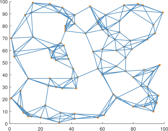
Following the work of qiu2017time , we generate $N=100$ nodes randomly from the uniform distribution in a $100\times 100$ square area. The graph weight is determined using $k$-nearest neighbors. Specifically, the weight between any two nodes is inversely proportional to the square of their Euclidean distance. We consider $k=5$ and visualize the corresponding graph in Fig. 1.

Figure 1: The graph is constructed by kNN with $k=5$. The weight between any two nodes is inversely proportional to the square of their Euclidean distance.

Denote the weight matrix by $W,$ its degree matrix $D,$ and the graph Laplacian $L$ has eigen-decomposition $L=U\Lambda U^{T},$ where $\Lambda=\text{diag}(0,\lambda_{2},\cdots,\lambda_{N})$. We further define $L^{-1/2}=U\Lambda^{-1/2}U^{T}$ where $\Lambda^{-1/2}=\text{diag}(0,\lambda_{2}^{-1/2},\cdots,\lambda_{N}^{-1/2})$. Starting from $x_{1},$ we generate the time-varying graph signal

$$x_{t}=x_{t-1}+L^{-1/2}f_{t},\quad\text{for }t=2,\cdots,T,$$ (19)

where $f_{t}$ is an i.i.d. Gaussian signal rescaled to $\|f_{t}\|_{2}=\kappa$ and $\kappa$ corresponds to a temporal smoothness of the signal. Stacking $\{x_{t}\}$ as a column vector, we obtain a data matrix $X=[x_{1},x_{2},\cdots,x_{T}]$. We generate a low-rank data matrix obtained by starting with an empty matrix $X$ and repeating $X=[X,x_{1},\cdots,x_{10},x_{10},x_{9},\cdots,x_{1}]$ 10 times, thus also getting a $100\times 200$ data matrix. The measurement noise at each node is i.i.d. Gaussian noise $\mathcal{N}(0,\eta^{2}),$ where $\eta$ is the standard deviation.

Parameter tuning. For the proposed Algorithm 1, we fix the following parameters: $k=3$ and $\theta=1.8$ in the definition of fractional-order derivative (4); $\sigma=10^{3}$ in the definition of the ERF regularization (3); $\epsilon=0.1$ and $r=3$ in the Sobolev graph Laplacian; and the step size $\rho=10^{-6}$ in the ADMM iterations (6). In each set of experiments, we carefully tune two parameters $(\alpha,\beta)$ that determine the weights for the spatial-temporal smoothness and the low-rankness, respectively, in the proposed model (5). We choose the best combination of $(\alpha,\beta)$ among $\alpha\in\{0,10^{-5},10^{-4},10^{-3},10^{-2},10^{-1},1,10\}$ and $\beta\in\{0,10^{-8},10^{-7},10^{-6},10^{-5},10^{-4},10^{-3},10^{-2},10^{-1},1,10\}$. As demonstrated in Table 1, some competing methods are special cases of the proposed models, and hence, we only tune the parameters $\alpha,\beta$ for these methods while keeping other parameters fixed.

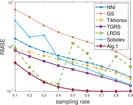
Reconstruction errors with respect to sampling rates. We begin by evaluating the performance of competing methods under different sampling rates. The smoothness level is set as $\kappa=1,$ while the standard deviation of the Gaussian noise is $\eta=0.1.$ The reconstruction performance is evaluated via RMSE, defined in (18), showing that the recovery errors of all the methods decrease with the increase of the sampling rates. The comparison results are visualized in Fig. 2. The proposed method achieves significant improvements over the competing methods. Surprisingly, LRDS, equipped with the nuclear norm, does not yield stable reconstruction performance in the low-rank case.

Figure 2: RMSE vs sampling rates. Averaged over 50 trials.

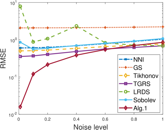
Reconstruction errors with respect to noise levels. We then investigate the recovery performance under different noise levels by setting the noise variance $\eta^{2}=\{0.01,0.1,0.2,0.4,0.6,0.8,1\}.$ In this set of experiments, we fix the sampling rate as 40% and smoothing level $\kappa=1.$ The noise level affects the magnitude of the least-squares fit, and as a result, we adjust the search window of $\alpha\in\{0,10^{-3},10^{-2},10^{-1},1,10,10^{2},10^{3},10^{4}$. The parameter $\beta$ remains the same: $\beta\in\{0,10^{-8},10^{-7},10^{-6},10^{-5},10^{-4},10^{-3},10^{-2},10^{-1},1,10\}$. The results are presented in Fig. 3, demonstrating the superior performance of the proposed Algorithm 1 under various noise levels.

Figure 3: RMSE vs noise level: $\eta^{2}=\{0.01,0.1,0.2,0.4,0.6,0.8,1\}.$ Averaged over 50 trials.

3.2 Real Data

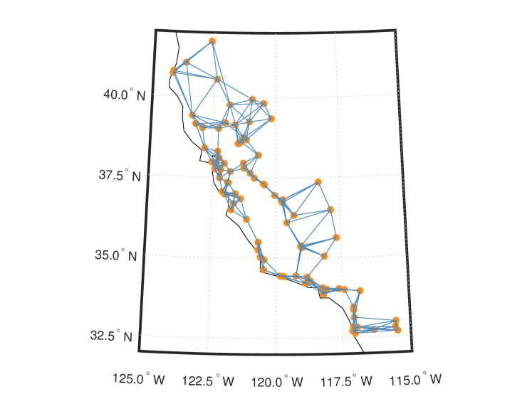
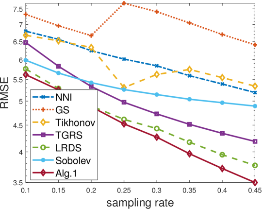
In the real data experiments, we first test the daily mean Particulate Matter (PM) 2.5 concentration dataset from California provided by the US Environmental Protection Agency https://www.epa.gov/outdoor-air-quality-data. We used the data captured daily from 93 sensors in California for the first 200 days in 2015. The constructed graph is depicted in Fig. 4. In Fig. 5, we compare the average recovery accuracy of all the comparing methods over 50 trials when the sampling rates are $0.1,0.15,0.2,0.25,0.3,0.35,0.4,0.45$. In Table 2, we also compare the performance of Algorithm 1 and Algorithm 2, which shows Algorithm 2 can improve the accuracy of Algorithm 1 under some sampling rates with longer time in general.

Figure 4: Graph with the places in California for the PM 2.5 concentration data. The graph was constructed with kNN for $k=5$.

Figure 5: Average recovery accuracy comparison on the PM2.5 data.

Sampling rate	Alg.1		Alg.2
	RMSE	Time (s)	RMSE	Time (s)
0.10	5.7321	22.95	5.6915	46.49
0.15	5.4770	22.63	6.4992	45.39
0.20	5.0427	23.83	5.9730	48.50
0.25	6.0358	23.37	5.6976	47.44
0.30	5.6065	23.70	5.3809	47.86
0.35	5.1920	23.55	5.1535	47.72
0.40	5.2398	23.56	4.7758	47.59
0.45	5.2283	23.80	5.0913	48.17

Table 2: Performance comparison of Algorithm 1 and Algorithm 2 for the PM2.5 data. The running time for Algorithm 1 is about 22$\sim$23 seconds while Algorithm 2 uses about $46\sim 48$ seconds.

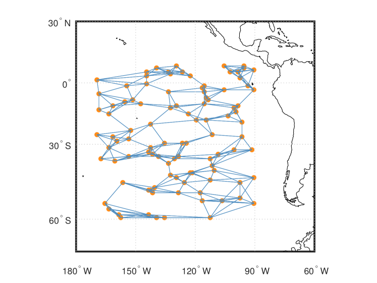
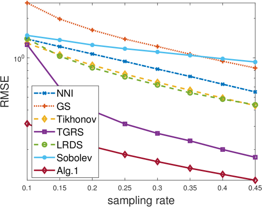
Next, we test the sea surface temperature dataset, which was captured monthly by the NOAA Physical Sciences Laboratory (PSL). The data set can be downloaded from the PSL website https://psl.noaa.gov/. We use a subset of 200 time points on the Pacific Ocean within 400 months. The constructed graph is illustrated in Fig. 6. We see from Fig. 7 that the proposed algorithm outperforms other methods significantly and consistently across all sampling rates. In Table 3, we also compare the performance of Algorithm 1 and Algorithm 2, which indicates Algorithm 2 can improve the accuracy of Algorithm 1 under certain sampling rates but with more computational time in general.

Figure 6: Graph with the places in the sea for the sea surface temperature data. The graph was constructed with kNN for $k=10$.

Figure 7: Average recovery accuracy comparison on the sea surface temperature data.

Sampling rate	Algorithm 1		Algorithm 2
	RMSE	Time (s)	RMSE	Time (s)
0.10	0.3148	3.97	0.3163	22.99
0.15	0.2497	3.37	0.2483	17.13
0.20	0.2110	3.08	0.2109	13.52
0.25	0.1832	2.87	0.1857	11.27
0.30	0.1617	2.74	0.1666	9.62
0.35	0.1438	2.63	0.1450	5.77
0.40	0.1294	2.54	0.1291	5.66
0.45	0.1166	2.46	0.1153	5.57

Table 3: Performance comparison of Algorithm 1 and Algorithm 2 for the sea surface temperature data. The running time for Algorithm 1 is about 2$\sim$4 seconds while Algorithm 2 uses about $6\sim 23$ seconds.

3.3 Discussions

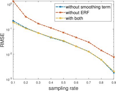
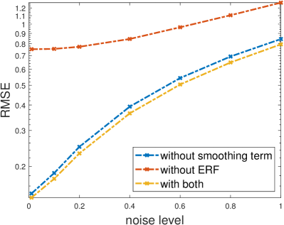
Using the sea surface temperature data, we conduct an ablation study of the proposed model (5) without the smoothing regularization by setting $\alpha=0$ or without the low-rank ERF term by setting $\beta=0$. We plot the RMSE curves with respect to the sampling rates and the noise levels in Fig. 8, showing that the ERF regularization has a larger influence on the performance compared to the Sobolev-base graph Laplacian regularization.

Figure 8: Ablation study sampling rates (left) and noise levels (right) on the sea surface temperature data.

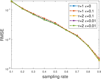
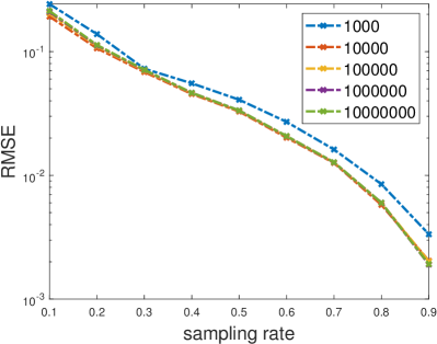
Using the same sea surface temperature data, we investigate whether the proposed model (5) is sensitive to the parameters $(r,\epsilon)$ in defining the Sobolev-graph Laplacian and $\sigma^{2}$ in defining the ERF regularization. Fig. 9 shows that the proposed approach is not sensitive to various degrees of smoothness controlled by $r$ and $\epsilon$. Although the ERF regularization plays an important role in the recovery performance, as illustrated in the ablation study, the proposed model is not sensitive to the choice $\sigma^{2}$ as long as it is larger than 10,000.

In addition, we compare the proposed Algorithm 1 and Algorithm 2 using the sea surface temperature data and show the results in Tables 2 and 3. One can see that the two algorithms lead to similar RMSE, but Algorithm 2 is slower overall. We therefore prefer to use Algorithm 1 unless the data is heavily polluted by the non-Gaussian type of noise, such as Laplace noise.

Figure 9: Sensitivity analysis with respect to varying the graph Laplacian (left) and $\sigma^{2}$ in ERF (right) on the Sea Surface Temperature data.

4 Conclusions and Future Work

In this paper, we exploit high-order smoothness across the temporal domain and adaptive low-rankness for time-varying graph signal recovery. In particular, we propose a novel graph signal recovery model based on a hybrid graph regularization involving a general order temporal difference, together with an error-function weighted nuclear norm. We also derive an effective optimization algorithm with guaranteed convergence by adopting a reweighting scheme and the ADMM framework. Numerical experiments have demonstrated their efficiency and performance in terms of accuracy. In the future, we will explore using high-order difference schemes to create a temporal Laplacian and low-rankness for recovering graph signals with dynamic graph topology.

References

- [1] David I Shuman, Sunil K Narang, Pascal Frossard, Antonio Ortega, and Pierre Vandergheynst. The emerging field of signal processing on graphs: Extending high-dimensional data analysis to networks and other irregular domains. IEEE signal processing magazine, 30(3):83–98, 2013.
- [2] Michael T Mills and Nikolaos G Bourbakis. Graph-based methods for natural language processing and understanding - a survey and analysis. IEEE Transactions on Systems, Man, and Cybernetics: Systems, 44(1):59–71, 2013.
- [3] Nicolas Tremblay and Pierre Borgnat. Graph wavelets for multiscale community mining. IEEE Transactions on Signal Processing, 62(20):5227–5239, 2014.
- [4] Aliaksei Sandryhaila and José MF Moura. Discrete signal processing on graphs. IEEE transactions on signal processing, 61(7):1644–1656, 2013.
- [5] Jhony H Giraldo and Thierry Bouwmans. On the minimization of sobolev norms of time-varying graph signals: estimation of new coronavirus disease 2019 cases. In 2020 IEEE 30th International Workshop on Machine Learning for Signal Processing (MLSP), pages 1–6. IEEE, 2020.
- [6] Siheng Chen, Aliaksei Sandryhaila, José MF Moura, and Jelena Kovačević. Signal recovery on graphs: Variation minimization. IEEE Transactions on Signal Processing, 63(17):4609–4624, 2015.
- [7] Ariel Kroizer, Yonina C Eldar, and Tirza Routtenberg. Modeling and recovery of graph signals and difference-based signals. In 2019 IEEE Global Conference on Signal and Information Processing (GlobalSIP), pages 1–5. IEEE, 2019.
- [8] Xiao Peng Li, Yi Yan, Ercan Engin Kuruoglu, Hing Cheung So, and Yuan Chen. Robust recovery for graph signal via -norm regularization. IEEE Signal Processing Letters, 2023.
- [9] Fei Chen, Gene Cheung, and Xue Zhang. Manifold graph signal restoration using gradient graph laplacian regularizer. IEEE Transactions on Signal Processing, 2024.
- [10] Rohan Varma, Siheng Chen, and Jelena Kovačević. Spectrum-blind signal recovery on graphs. In 2015 IEEE 6th International Workshop on Computational Advances in Multi-Sensor Adaptive Processing (CAMSAP), pages 81–84. IEEE, 2015.
- [11] João Domingos and José MF Moura. Graph fourier transform: A stable approximation. IEEE Transactions on Signal Processing, 68:4422–4437, 2020.
- [12] Cuneyd Ozturk, Haldun M Ozaktas, Sinan Gezici, and Aykut Koç. Optimal fractional fourier filtering for graph signals. IEEE Transactions on Signal Processing, 69:2902–2912, 2021.
- [13] Wang Ying, Xu Rui, Ma Xiaoyang, Fu Qiang, Zhao Jinshuai, and Zhou Runze. Spectral graph theory-based recovery method for missing harmonic data. IEEE Transactions on Power Delivery, 37(5):3688–3697, 2021.
- [14] Peter Berger, Gabor Hannak, and Gerald Matz. Graph signal recovery via primal-dual algorithms for total variation minimization. IEEE Journal of Selected Topics in Signal Processing, 11(6):842–855, 2017.
- [15] Junzheng Jiang, David B Tay, Qiyu Sun, and Shan Ouyang. Recovery of time-varying graph signals via distributed algorithms on regularized problems. IEEE Transactions on Signal and Information Processing over Networks, 6:540–555, 2020.
- [16] Feng Xia, Ke Sun, Shuo Yu, Abdul Aziz, Liangtian Wan, Shirui Pan, and Huan Liu. Graph learning: A survey. IEEE Transactions on Artificial Intelligence, 2(2):109–127, 2021.
- [17] Robin Sibson. A brief description of natural neighbour interpolation. Interpreting multivariate data, pages 21–36, 1981.
- [18] Sunil K Narang, Akshay Gadde, Eduard Sanou, and Antonio Ortega. Localized iterative methods for interpolation in graph structured data. In 2013 IEEE Global Conference on Signal and Information Processing, pages 491–494. IEEE, 2013.
- [19] Kai Qiu, Xianghui Mao, Xinyue Shen, Xiaohan Wang, Tiejian Li, and Yuantao Gu. Time-varying graph signal reconstruction. IEEE Journal of Selected Topics in Signal Processing, 11(6):870–883, 2017.
- [20] Nathanaël Perraudin, Andreas Loukas, Francesco Grassi, and Pierre Vandergheynst. Towards stationary time-vertex signal processing. In 2017 IEEE International Conference on Acoustics, Speech and Signal Processing (ICASSP), pages 3914–3918. IEEE, 2017.
- [21] Xianghui Mao, Kai Qiu, Tiejian Li, and Yuantao Gu. Spatio-temporal signal recovery based on low rank and differential smoothness. IEEE Transactions on Signal Processing, 66(23):6281–6296, 2018.
- [22] Jhony H Giraldo, Arif Mahmood, Belmar Garcia-Garcia, Dorina Thanou, and Thierry Bouwmans. Reconstruction of time-varying graph signals via sobolev smoothness. IEEE Transactions on Signal and Information Processing over Networks, 8:201–214, 2022.
- [23] Jinling Liu, Jiming Lin, Hongbing Qiu, Junyi Wang, and Liping Nong. Time-varying signal recovery based on low rank and graph-time smoothness. Digital Signal Processing, 133:103821, 2023.
- [24] Hayate Kojima, Hikari Noguchi, Koki Yamada, and Yuichi Tanaka. Restoration of time-varying graph signals using deep algorithm unrolling. In ICASSP 2023-2023 IEEE International Conference on Acoustics, Speech and Signal Processing (ICASSP), pages 1–5. IEEE, 2023.
- [25] Jhon A Castro-Correa, Jhony H Giraldo, Anindya Mondal, Mohsen Badiey, Thierry Bouwmans, and Fragkiskos D Malliaros. Time-varying signals recovery via graph neural networks. In ICASSP 2023-2023 IEEE International Conference on Acoustics, Speech and Signal Processing (ICASSP), pages 1–5. IEEE, 2023.
- [26] Zhenlong Xiao, He Fang, Stefano Tomasin, Gonzalo Mateos, and Xianbin Wang. Joint sampling and reconstruction of time-varying signals over directed graphs. IEEE Transactions on Signal Processing, 2023.
- [27] Weihong Guo, Yifei Lou, Jing Qin, and Ming Yan. A novel regularization based on the error function for sparse recovery. Journal of Scientific Computing, 87(1):1–22, 2021.
- [28] Shuhang Gu, Lei Zhang, Wangmeng Zuo, and Xiangchu Feng. Weighted nuclear norm minimization with application to image denoising. In Proceedings of the IEEE conference on computer vision and pattern recognition, pages 2862–2869, 2014.
- [29] Emmanuel J Candes, Michael B Wakin, and Stephen P Boyd. Enhancing sparsity by reweighted minimization. Journal of Fourier analysis and applications, 14(5):877–905, 2008.
- [30] Igore Podlubny. Fractional differential equations. Mathematics in science and engineering, 198:41–119, 1999.