Pseudoentropy sum rule by analytical continuation of the superposition parameter

Abstract

In this paper, we establish a sum rule that connects the pseudoentropy and entanglement entropy of a superposition state. Through analytical continuation of the superposition parameter, we demonstrate that the transition matrix and density matrix of the superposition state can be treated in a unified manner. Within this framework, we naturally derive sum rules for the (reduced) transition matrix, pseudo-Rényi entropy, and pseudoentropy. Furthermore, we demonstrate the close relationship between the sum rule for pseudoentropy and the singularity structure of the entropy function for the superposition state after analytical continuation. We also explore potential applications of the sum rule, including its relevance to understanding the gravity dual of non-Hermitian transition matrices and establishing upper bounds for the absolute value of pseudoentropy.

School of Physics, Huazhong University of Science and Technology,
Luoyu Road 1037, Wuhan, Hubei 430074, China

1 Introduction

For a given quantum system, the wave function or density matrix is expected to include all the information about the system. In finite-dimensional Hilbert spaces, one can explicitly express the wave function using a complete basis. However, in the realms of quantum field theories (QFTs) and quantum many-body systems, obtaining the exact wave function with a given basis is often infeasible. Instead, we typically study the properties of the wave function by probing the entanglement or quantum correlations among different partitions.

In recent years, entanglement entropy (EE) has been a very useful quantity in various research fields[1]-[4]. Specially, in QFTs it is found to show some universal properties. In the context of AdS/CFT, EE is found to be linked to the bulk minimal surface, known as RT [5] or HRT formula [6], which gives us more insights into the nature of classical and quantum spacetime [7]-[12].

It is anticipated that the RT or HRT formula should extend beyond its application solely in AdS/CFT to encompass a broader framework of gauge/gravity duality, such as dS/CFT[13][14]. An important observation is that when applying the RT or HRT formula to more general scenarios, it may yield complex-valued results on the gravity side[15]. This implies that the dual quantity in boundary theories cannot be straightforwardly interpreted as EE. Thus, it suggests the necessity of generalizing the concept of EE to encompass a wider range of situations.

A proper way to generalize EE is by transitioning from the density matrix to what is known as the transition matrix[16]. In standard quantum mechanics, a system is characterized by the state $|\psi\rangle$, or by the density matrix $\rho=|\psi\rangle\langle\psi|$. The transition matrix incorporates another state $|\phi\rangle$, thereby extending the density matrix $\rho$ to non-Hermitian $\mathcal{T}^{\psi|\phi}=\frac{|\psi\rangle\langle\phi|}{\langle\phi|\psi\rangle}$. The non-Hermitian transition matrix exhibits very similar properties to the density matrix. If one can describe the system using the transition matrix, we can define the reduced transition matrix for subsystem $A$

$$\mathcal{T}_{A}^{\psi|\phi}:=tr_{\bar{A}}\mathcal{T}^{\psi|\phi},$$ (1)

where $\bar{A}$ is the complementary part of $A$. Subsequently, we can define the quantity $S(\mathcal{T}_{A}^{\psi|\phi}):=-tr\mathcal{T}_{A}^{\psi|\phi}\log\mathcal{T}_{A}^{\psi|\phi}$ as a generalization of von Neumann entropy of $\rho_{A}:=tr\rho$[16], see also [17]. $S(\mathcal{T}_{A}^{\psi|\phi})$ is referred to as pseudoentropy (PE), and it is generally complex-valued. To compute PE we usually introduce the pseudo-Rényi entropy $S^{(n)}(\mathcal{T}_{A}^{\psi|\phi})=\frac{\log tr(\mathcal{T}_{A}^{\psi|\phi})^{n}}{1-n}$ for $n$ being integers. The PE can be obtained by analytical continuation of $n$ and taking the limit $S(\mathcal{T}_{A}^{\psi|\phi})=\lim_{n\to 1}S^{(n)}(\mathcal{T}_{A}^{\psi|\phi})$.

A common question regarding the concept of PE is whether it can be interpreted as a type of entropy. This is actually a subtle question. On one hand, EE can be seen as a special case when $|\phi\rangle=|\psi\rangle$. On the other hand if one insist the RT or HRT formula can be applied to more general situations, it is nature to introduce the transition matrix and PE in QFTs. On the other hand, if one insists that the RT or HRT formula can be applied to more general situations, it is natural to introduce the transition matrix and PE in QFTs. Furthermore, recent findings have revealed that the transition matrix is inherently linked to the density matrix of the superposition state[37]. To state the relation we would like to introduce a series of superposition states denoted by $|\xi(c)\rangle$, defined as

$$|\xi(c)\rangle=\mathcal{N}(c)(|\phi\rangle+c|\psi\rangle),$$ (2)

where $\mathcal{N}(c)=1/\sqrt{1+|c|^{2}+c\langle\phi|\psi\rangle+c^{*}\langle\psi|\phi\rangle}$ is the normalization constant for the state $|\xi(c)\rangle$. We also define the reduced density matrix $\rho_{A}(c):=\textrm{tr}_{\bar{A}}|\xi(c)\rangle\langle\xi(c)|$. It is expected that we can establish the following relations connecting the operator $\mathcal{T}_{A}^{\psi|\phi}$ and $\rho_{A}(c)$,

$$(\mathcal{T}_{A}^{\psi|\phi})^{n}=\sum_{c\in\mathcal{S}}a(c)[\rho_{A}(c)]^{n},$$ (3)

where $a(c)$ are n-dependent constants, the index $c$ belongs to a given set denoted by $\mathcal{S}$.

The sum rule (3) implies that the transition matrix is connected to the density matrix in a precise manner. This operator sum rule enables the derivation of a relationship between pseudo-Rényi entropy and Rényi entropy. Consequently, it offers a pathway to comprehend the physical significance of pseudo-Rényi entropy and PE. In [37] we construct a sum rule for the pseudo-Rényi entropy by using discrete Fourier transformation. For the sake of comparison, let’s introduce the sum rule given in [37]. The superposition states are given by

$$|\xi_{k}\rangle=\mathcal{N}(e^{\frac{2\pi i}{2n+1}k})(|\phi\rangle+e^{\frac{2\pi i}{2n+1}k}|\psi\rangle),$$ (4)

where $\mathcal{N}(e^{\frac{2\pi i}{2n+1}k})=1/\sqrt{2+e^{\frac{2\pi i}{2n+1}k}\langle\phi|\psi\rangle+e^{-\frac{2\pi i}{2n+1}k}\langle\psi|\phi\rangle}$. The operator sum rule is

$$(\mathcal{T}_{A}^{\psi|\phi})^{n}=\sum_{k=0}^{2n}a_{k}[\rho_{A}(k)]^{n},$$ (5)

with

$$a_{k}:=a(\mathrm{e}^{\frac{2\pi\mathrm{i}}{2n+1}k})=\frac{\mathrm{e}^{-\frac{2\pi\mathrm{i}}{2n+1}kn}}{(2n+1){{\mathcal{N}}_{k}^{n}}},\quad{\mathcal{N}}_{k}:=\mathcal{N}(\mathrm{e}^{\frac{2\pi\mathrm{i}}{2n+1}k})^{2}\langle\phi|\psi\rangle,$$ (6)

where $\rho_{A}(k):=\rho_{A}(\mathrm{e}^{\frac{2\pi\mathrm{i}}{2n+1}k})$.

As emphasized in [37], the form of the sum rule is not unique and depends on the choices of the set $\mathcal{S}$. Other forms of the sum rule can be obtained by appropriately selecting the set $\mathcal{S}$ and coefficients $a(c)$. However, the sum rule derived in [37] does not smoothly converge to the pseudoentropy in the limit as $n$ approaches 1. In this paper, we demonstrate that the sum rule for pseudo-Rényi entropy can also be expressed in integral form by using the Fourier transformation. Furthermore, we utilize this result to derive a sum rule for pseudoentropy.

More importantly, through the construction of the new form sum rule, we discover that the transition matrix and density matrix of a superposition state can be treated in a unified manner. This is achieved by analytically continuing the real superposition parameter to complex values. In this framework, the transition matrix can be obtained through contour integration at infinity. Using the properties of complex integration, the sum rule for the transition matrix, pseudo-Rényi entropy, and PE can be derived naturally. In fact, this approach can be readily extended to other quantities defined by the transition matrix.

2 A new form sum rule

In this paper we would like to consider the superposition state

$$|\xi(\theta)\rangle=\mathcal{N}(\theta)(|\phi\rangle+e^{i\theta}|\psi\rangle),$$ (7)

where $\theta\in(-\pi,\pi)$ and $\mathcal{N}(\theta)=1/\sqrt{2+e^{i\theta}\langle\phi|\psi\rangle+e^{-i\theta}\langle\psi|\phi\rangle}$ is the normalization constant. The new sum rule is expressed as

$$(\mathcal{T}_{A}^{\psi|\phi})^{n}=\frac{1}{2\pi}\int_{-\pi}^{\pi}d\theta e^{-in\theta}\mathcal{N}_{\theta}^{n}\rho_{A}(\theta)^{n},$$ (8)

where $\mathcal{N}_{\theta}:=\mathcal{N}(\theta)^{-2}\langle\phi|\psi\rangle^{-1}$. The form of the above sum rule is very similar to the one (5). Here, we derive the result using Fourier transformation. Its advantages will become clear in the following sections.

Using the operator sum rule (8) one could establish sum rule for the pseudo-Rényi entropy and off-diagonal matrix elements as we have done in [37]. The pseudo-Rényi entropy sum rule is easy to obtain by taking trace on both side of (8), the result is

$$\mathrm{e}^{(1-n)S^{(n)}(\mathcal{T}_{A}^{\psi|\phi})}=\frac{1}{2\pi}\int_{-\pi}^{\pi}d\theta e^{-in\theta}\mathcal{N}_{\theta}^{n}\mathrm{e}^{(1-n)S^{(n)}(\rho_{A}(\theta))}.$$ (9)

Consider a set of operators $\{\mathcal{A}_{j}\}$ (j=1,…,m) located in the subsystem $A$. If $m\leq n$ we would have the following interesting relations

$$\prod_{j=1}^{m}\frac{\langle\phi|\mathcal{A}_{j}|\psi\rangle}{\langle\phi|\psi\rangle}=\frac{1}{2\pi}\int_{-\pi}^{\pi}d\theta e^{-in\theta}\mathcal{N}_{\theta}^{n}\prod_{j=1}^{m}\langle\xi(\theta)|\mathcal{A}_{j}|\xi(\theta)\rangle.$$ (10)

The formula above demonstrates that the off-diagonal elements $\langle\phi|\mathcal{A}|\psi\rangle$ can be related to the diagonal ones $\langle\xi(\theta)|\mathcal{A}_{j}|\xi(\theta)\rangle$. This relation can be directly verified using the properties of Fourier transformation. In quantum field theory, it can also be derived by employing replica methods to evaluate the pseudo-Rényi entropy. Eq.(10) is closely connected to Eq.(9) in this context.

2.1 Proof of the operator sum rule

Although the proof of the new operator sum rule (8) closely resembles the one in [37], for the sake of completeness, we will briefly outline the proof here. The key step is that $\rho_{A}(c)$ can be expanded as follows,

$$\rho_{A}(c)=\mathcal{N}(c)^{2}\big{(}\rho_{A}^{\phi}+c\langle\phi|\psi\rangle\mathcal{T}_{A}^{\psi|\phi}+c^{*}\langle\psi|\phi\rangle\mathcal{T}_{A}^{\phi|\psi}+cc^{*}\rho_{A}^{\psi}\big{)},$$ (11)

where $\rho_{A}^{\phi}:=\textrm{tr}_{\bar{A}}|\phi\rangle\langle\phi|$, and $\rho_{A}^{\psi}:=\textrm{tr}_{\bar{A}}|\psi\rangle\langle\psi|$. The $n$-th power of $\rho_{A}(c)$ should include polynomial terms involving four operators on the right-hand side of (11).

$$[\rho_{A}(c)]^{n}=\sum_{\{r,s,t\}}c^{t+r}(c^{*})^{s+r}\langle\phi|\psi\rangle^{t}\langle\psi|\phi\rangle^{s}\mathcal{N}(c)^{2n}\{(\rho_{A}^{\phi})^{n-r-s-t}(\mathcal{T}_{A}^{\psi|\phi})^{t}(\mathcal{T}_{A}^{\phi|\psi})^{s}(\rho^{\psi}_{A})^{r}$$

$$\phantom{[\rho_{A}(c)]^{n}=\sum_{\{r,s,t\}}}+\cdots\},$$ (12)

where $``+\cdots"$ denotes the sum of all possible permutation terms for each fixed $r,s,t$. One of the special term in the summation is the one with $t=n,s=0,r=0$, i.e., $(\mathcal{T}_{A}^{\psi|\phi})^{n}$. One could consider the linear combination of $[\rho_{A}(c)]^{n}$ as the right hand side of (3). The key point is that it is possible for only the special terms $(\mathcal{T}_{A}^{\psi|\phi})^{n}$ to remain while all others disappear. To achieve this we require the condition

$$\sum_{c\in\mathcal{S}}a(c)c^{t+r}(c^{*})^{s+r}\langle\phi|\psi\rangle^{t}\langle\psi|\phi\rangle^{s}\mathcal{N}(c)^{2n}=\delta_{s,0}\delta_{t,n},$$ (13)

Now we would like to consider a continuous set $\mathcal{S}=\{e^{i\theta}\}$ with $\theta\in(-\pi,\pi)$. The summation in (13) should be replaced by integration over the interval $(-\pi,\pi)$. We have the equation

$$\int_{-\pi}^{\pi}d\theta f(\theta)\mathrm{e}^{i(t-s-n)\theta}=\delta_{s,0}\delta_{t,n},$$ (14)

where

$$f(\theta):=a(\mathrm{e}^{i\theta})\left[e^{i\theta}\mathcal{N}(\mathrm{e}^{i\theta})^{2}\langle\phi|\psi\rangle\right]^{n}.$$ (15)

The solution to the above equation is $f(\theta)=\frac{1}{2\pi}$, from which we can obtain $a(e^{i\theta})$. Thus, we have established the validity of the new operator sum rule (8). Through a similar treatment, one could also derive an operator sum rule for the case where $|\psi\rangle$ and $|\phi\rangle$ are orthogonal.

Let us discuss why the term $(\mathcal{T}_{A}^{\psi|\phi})^{n}$ is particularly significant. The summation terms on the right hand side of (2.1) actually contain many interesting terms that can be utilized to derive other measures of information. One example is the term $(\rho_{A}^{\phi})^{n-1}\rho_{A}^{\psi}$, which is employed in [51] to compute the relative entropy for the density matrices $\rho_{A}^{\phi}$ and $\rho_{A}^{\psi}$. This term corresponds to $t=s=0$ and $r=1$ in the summation in (2.1). In general, we can parameterize the index $c$ as $Re^{i\theta}$, where $R\in(0,+\infty)$ and $\theta\in(0,2\pi)$. The coefficients associated with fixed $t,s,r$ in the summation of Eq.(2.1) are given by

$$R^{2r+t+s}e^{i(t-s)\theta}\langle\phi|\psi\rangle^{t}\langle\psi|\phi\rangle^{s}\mathcal{N}(Re^{i\theta})^{2n}.$$ (16)

The term $(\rho_{A}^{\phi})^{n-1}\rho_{A}^{\psi}$ corresponds to the case $t=s=0,r=1$.Its coefficient is same with the terms corresponding to $t=s=1,r=0$, that is $(\rho_{A}^{\phi})^{n-2}\mathcal{T}_{A}^{\psi|\phi}\mathcal{T}_{A}^{\phi|\psi}$ along with all their possible permutations. Consequently, isolating the term $(\rho_{A}^{\phi})^{n-1}\rho_{A}^{\psi}$ using the method we previously discussed is not feasible.

2.2 Analytical continuation of the superposition parameter

The sum rule (8) can also be seen as a natural result by analytical continuation of the superposition parameter $\theta$ of the state $|\xi(\theta)\rangle$. Let us consider the unnormalized state

$$|\tilde{\xi}(\theta)\rangle=|\phi\rangle+e^{i\theta}|\psi\rangle,$$ (17)

and the density matrix

$$\tilde{\rho}(\theta)=|\tilde{\xi}(\theta)\rangle\langle\tilde{\xi}(\theta)|=(|\phi\rangle+e^{i\theta}|\psi\rangle)(\langle\phi|+e^{-i\theta}\langle\psi|).$$ (18)

If $\theta$ lies in the interval $(-\pi,\pi)$, the operator $\tilde{\rho}(\theta)$ is Hermitian. We can treat $\tilde{\rho}(\theta)$ as a function of a real parameter $\theta$. Now, we aim to perform an analytical continuation of $\theta$ to arbitrary complex values, akin to the Wick rotation method employed in quantum field theory. The result is

$$\tilde{\rho}(z)=(|\phi\rangle+z|\psi\rangle)(\langle\phi|+\frac{1}{z}\langle\psi|),$$ (19)

where $z$ is complex. The function $\tilde{\rho}(z)$ is defined on the complex plane, with the density matrix $\tilde{\rho}(\theta)$ lying specifically on the unit circle $|z|=1$. It’s worth noting that $\tilde{\rho}(z)$ is Hermitian only when evaluated on points lying on the unit circle $|z|=1$.

$\tilde{\rho}(z)$ has simple poles at $z=0$ and $z=\infty$. One could extract the off-diagonal element $|\phi\rangle\langle\psi|$ by using the integral

$$|\phi\rangle\langle\psi|=\frac{1}{2\pi i}\oint_{C}dz\tilde{\rho}(z),$$ (20)

where $C$ represents an arbitrary closed counterclockwise contour enclosing the point $z=0$, see Fig.1. Similarly, we have

$$|\psi\rangle\langle\phi|=\frac{1}{2\pi i}\oint_{C}dz\frac{1}{z^{2}}\tilde{\rho}(z),$$ (21)

where $C$ denotes the same contour shown in Fig.1. The contours $C$ can be deformed to the unit circle $|z|=1$. One could also extract $|\psi\rangle\langle\phi|$ from the pole at infinity $z=\infty$, that is

$$|\psi\rangle\langle\phi|=\frac{1}{2\pi i}\oint_{C}dz\tilde{\rho}(1/z),$$ (22)

where $C$ is again the contour surrounding $z=0$. we can derive the density matrix under the dephasing channel as

$$|\phi\rangle\langle\phi|+|\psi\rangle\langle\psi|=\frac{1}{2\pi i}\oint_{C}z^{-1}\tilde{\rho}(z).$$ (23)

By changing the coordinate $z=e^{i\theta}$ the off-diagonal elements $|\phi\rangle\langle\psi|$ and $|\psi\rangle\langle\phi|$ can be written as linear combinations of the density matrix $\tilde{\rho}(\theta)$.

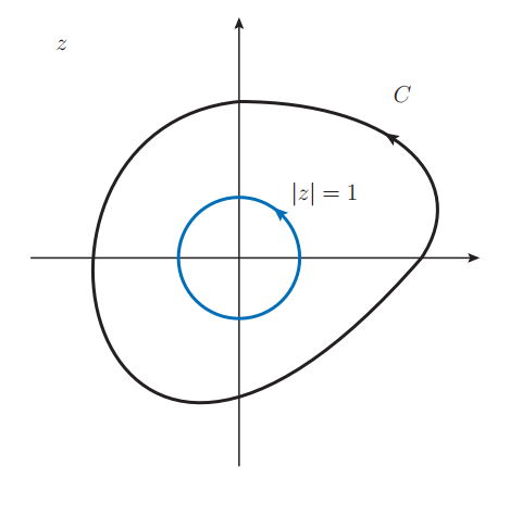
Figure 1: The contours for evaluating the integral (20) and (21) on the complex $z$ plane. The contour can be deformed to the unit circle (depicted in blue).

The sum rule (8) can be understood by similar way. The first step is to define the reduced operator $\tilde{\rho}_{A}(z):=tr_{\bar{A}}\tilde{\rho}(z)$. $\tilde{\rho}_{A}(z)$ and its n-th power $(\tilde{\rho}_{A}(z))^{n}$ with $n$ being integers are both meromorphic functions. By calculation we have

$$(\tilde{\rho}_{A}(z))^{n}=z^{n}(\tilde{\mathcal{T}}_{A}^{\psi|\phi})^{n}+...,$$ (24)

where $\tilde{\mathcal{T}}_{A}^{\psi|\phi}:=tr_{\bar{A}}|\psi\rangle\langle\phi|$, “+…” represents terms involving powers of $z$ less than $n$. Thus we obtain

$$(\tilde{\mathcal{T}}_{A}^{\psi|\phi})^{n}=\frac{1}{2\pi i}\oint_{C}z^{-n-1}(\tilde{\rho}_{A}(z))^{n}dz.$$ (25)

Specially, the contour $C$ can be chosen as the unit circle $|z|=1$. This choice results in the operator sum rule (8) upon restoring the normalization constants for $\tilde{\mathcal{T}}_{A}^{\psi|\phi}$ and $\tilde{\rho}_{A}(z)$. Define $\rho(z)=\mathcal{N}(z)\tilde{\rho}(z)$, with $\mathcal{N}(z)=z(2z+z^{2}\langle\phi|\psi\rangle+\langle\psi|\phi\rangle)^{-1}$, we have

$$(\mathcal{T}_{A}^{\psi|\phi})^{n}=\frac{1}{2\pi i}\oint_{C}z^{-n-1}\mathcal{N}_{z}^{n}\rho(z)^{n}dz,$$ (26)

where $\mathcal{N}_{z}=\mathcal{N}(z)^{-1}\langle\phi|\psi\rangle^{-1}$. Taking $z=e^{i\theta}$ we obtain the sum rule (8).

The above discussion can be extended to more general cases. We begin with the function $\tilde{\rho}(z)$ which has simple poles on the complex $z$ plane. The function $(\tilde{\rho}(z)_{A})^{n}$ stands out due to the specific operations of partial trace and taking the $n$-th power. Indeed, it remains a meromorphic function, with its poles clearly identifiable. In general, the inclusion of more generalized quantum channel operations $\mathcal{R}(\tilde{\rho})$ may lead to result functions that are not meromorphic. These functions could possess more intricate singularity structures, such as branch cuts. In such cases, careful consideration of the chosen contours becomes imperative. In the following we will show the entanglement entropy as examples.

The analytical continuation of the superposition parameter can indeed be extended to multiple superposition states. For instance,

$$\tilde{\rho}(\theta_{1},...,\theta_{m}):=\sum_{k=1}^{m}\sum_{k^{\prime}=1}^{m}e^{i\theta_{k}}|\psi_{k}\rangle\langle\psi_{k^{\prime}}|e^{-i\theta_{k^{\prime}}}$$ (27)

By extending the real parameters $\{\theta_{k}\}$ ($k=1,...,m$) to complex values, we obtain a function $\tilde{\rho}(z_{1},...,z_{m})$ defined on multiple complex variables $z_{1},...,z_{m}$.

3 Pseudo entropy sum rule

3.1 An approximated sum rule

In [37] by using the formula (5) for pseudo-Rényi entropy, we derive a tentative sum rule for pseudoentropy, which is given by

$$S(\mathcal{T}_{A}^{\psi|\phi})=\sum_{k=0}^{2}\frac{\mathrm{e}^{-\frac{2\pi\mathrm{i}}{3}k}}{3\langle\phi|\psi\rangle}\frac{S(\rho_{A}(k))|_{n=1}}{[\mathcal{N}(\mathrm{e}^{\frac{2\pi\mathrm{i}}{3}k})]^{2}}.$$ (28)

However, we have shown in [37] the sum rule for pseudoentropy is not correct for general cases. It is only applicable if the distance between the two states $|\psi\rangle$ and $|\phi\rangle$ is small. For example $|\phi\rangle\propto|\psi\rangle+\epsilon|\psi^{\prime}\rangle$, where $\epsilon\ll 1$, the above sum rule (28) is correct at the leading order of $\epsilon$. This actually means the pseudoentropy also satisfy the first-law like relation at leading order of the perturbation[37].

3.2 A method to obtain entanglement entropy from Rényi entropy

It is easy to check the sum rule (8) for $n$ being integers. But it would be subtle to analytically extend $n$ to complex numbers. To avoid this, we would like to use a method to extract entanglement entropy from Rényi entropy without analytical continuation of $n$, which is introduced in [52].

Firstly, let us briefly review this method. For a given density matrix $\rho$, suppose we know the trace of powers of $\rho$,

$$R_{n}(\rho)=tr\rho^{n},$$ (29)

for the integers $n>1$. The strategy is to introduce the generating function

$$G(z,\rho)=-tr\left(\rho\log\frac{1-z\rho}{1-z}\right)=\sum_{n=2}\frac{z^{n-1}}{n-1}\left[R_{n}(\rho)-1\right],$$ (30)

where the series is convergent in the unit disc $|z|<1$. The function $G(z,\rho)$ can be analytically continued to the cut plane $C\backslash[1,\infty)$, where $[1,\infty)$ is the branch cut of the logarithm. It can be shown one could obtain entanglement entropy by

$$S(\rho):=-tr\rho\log\rho=\lim_{z\to-\infty}G(z,\rho).$$ (31)

One could generalize the above method to the transition matrix $\mathcal{T}$, which is in general non-hermitian. One could also define the generating function $G(z,\mathcal{T})$ by replacing $\rho$ with $\mathcal{T}$ in (30). In our approach, the operator $\mathcal{T}$ would be normalized to $tr(\mathcal{T})=1$. One could similarly define the generating function

$$G(z,\mathcal{T})=-tr\left(\mathcal{T}\log\frac{1-z\mathcal{T}}{1-z}\right).$$ (32)

Suppose the series expansion like (30) is convergent in the disc $|z|<1$. Then the function $G(z,\mathcal{T})$ can be analytically continued to the cut plane $C\backslash[1,\infty)$. Similarly, one could obtain the pseudoentropy by

$$S(\mathcal{T}):=-tr\mathcal{T}\log\mathcal{T}=\lim_{z\to-\infty}G(z,\mathcal{T}).$$ (33)

3.3 Derivation of the sum rule

By using the new sum rule (8) and the definition of generating function $G$, we have

$$G(z,\mathcal{T}_{A}^{\psi|\phi})=\sum_{n=2}^{\infty}\frac{z^{n-1}}{n-1}\left[\frac{1}{2\pi}\int_{-\pi}^{\pi}d\theta e^{-in\theta}\mathcal{N}_{\theta}^{n}tr\rho_{A}(\theta)^{n}-1\right]$$

$$\phantom{G(z,\mathcal{T}_{A}^{\psi|\phi})}=\frac{1}{2\pi}\int_{-\pi}^{\pi}d\theta\sum_{n=2}^{\infty}\frac{z^{n-1}}{n-1}e^{-in\theta}\mathcal{N}_{\theta}^{n}tr\rho_{A}(\theta)^{n}-\sum_{n=2}^{\infty}\frac{z^{n-1}}{n-1}$$

$$\phantom{G(z,\mathcal{T}_{A}^{\psi|\phi})}=\frac{1}{2\pi}\int_{-\pi}^{\pi}d\theta G[z^{\prime},\rho(\theta)]e^{-i\theta}\mathcal{N}_{\theta}+\frac{1}{2\pi}\int_{-\pi}^{\pi}d\theta\left[\sum_{n=2}^{\infty}\frac{z^{\prime n-1}}{n-1}e^{-i\theta}\mathcal{N}_{\theta}-\sum_{n=2}^{\infty}\frac{z^{n-1}}{n-1}\right],$$

(34)

where $z^{\prime}:=ze^{-i\theta}\mathcal{N}_{\theta}$. Taking the limit $z\to-\infty$ on both side of the above equation, we have

$$S(\mathcal{T}_{A}^{\psi|\phi})=\frac{1}{2\pi}\int_{-\pi}^{\pi}d\theta e^{-i\theta}\mathcal{N}_{\theta}S[\rho(\theta)]+\frac{1}{2\pi}\lim_{z\to-\infty}\int_{-\pi}^{\pi}d\theta\left[\sum_{n=2}^{\infty}\frac{z^{n-1}}{n-1}e^{-in\theta}\mathcal{N}_{\theta}^{n}-\sum_{n=2}^{\infty}\frac{z^{n-1}}{n-1}\right],$$ (35)

where we have assumed the order of integration and limit can be exchanged. Further we have

$$\int_{-\pi}^{\pi}d\theta e^{-in\theta}\mathcal{N}_{\theta}^{n}=\int_{-\pi}^{\pi}d\theta e^{-in\theta}\left(2+e^{i\theta}\langle\phi|\psi\rangle+e^{-i\theta}\langle\psi|\phi\rangle\right)^{n}\langle\phi|\psi\rangle^{-n}=1.$$ (36)

Note that we have used the fact that $n$ is an integer. Thus the second term is vanishing. Finally, we obtain the sum rule for pseudoentropy

$$S(\mathcal{T}_{A}^{\psi|\phi})=\frac{1}{2\pi}\int_{-\pi}^{\pi}d\theta e^{-i\theta}\mathcal{N}_{\theta}S[\rho_{A}(\theta)].$$ (37)

As we will demonstrate below, the above sum rule for PE is only valid for some special cases.

The usual approach to obtain the EE or PE is through the analytical continuation of $n\to 1$. Actually, taking derivative with respect to $n$ on both side of (8) we would obtain a different result. By definition we have $S(\mathcal{T}_{A}^{\psi|\phi})=-\partial_{n}tr(\mathcal{T}_{A}^{\psi|\phi})^{n}|_{n=1}$. On the right-hand side of (8) we would have

$$\frac{1}{2\pi}\int_{-\pi}^{\pi}d\theta e^{-i\theta}\mathcal{N}_{\theta}S[\rho_{A}(\theta)]+\frac{1}{2\pi}\int_{-\pi}^{\pi}d\theta e^{-i\theta}\mathcal{N}_{\theta}\log[e^{-i\theta}\mathcal{N}_{\theta}].$$ (38)

Comparing with (37), there exists an additional term that generally does not vanish. This implies that the integrand on the right-hand side of (8) cannot be analytically continued to arbitrary $n$. However, in the approach utilizing the generating functions $G(z,\mathcal{T})$ and $G(z,\rho(\theta))$, we consistently maintain $n$ as an integer.

3.4 Methods by analytical continuation of superposition parameter

We can also express the sum rule by Cauchy integral. Define $\zeta=e^{i\theta}$, we have

$$S(\mathcal{T}_{A}^{\psi|\phi})=\frac{1}{2\pi i}\oint_{|\zeta|=1}\mathcal{N}_{\zeta}S(\rho_{A}(\zeta))d\zeta,$$ (39)

where $\mathcal{N}_{\zeta}:=\zeta^{-2}(2+\zeta\langle\phi|\psi\rangle+\zeta^{-1}\langle\psi|\phi\rangle)\langle\phi|\psi\rangle^{-1}$ and $S(\rho(\zeta)):=S(\rho_{A}(\theta))|_{\theta=-i\log\zeta}$. Here, we assume that the function $\mathcal{N}_{\zeta}S(\rho_{A}(\zeta))$ is a meromorphic function within the unit circle $|\zeta|\leq 1$. In general, $S(\rho_{A}(\zeta))$ may involve logarithmic functions, and it seems necessary to consider the branch cut of the logarithmic function for consistency. However, in certain cases, one can expand $S(\rho_{A}(\zeta))$ as polynomials of $\zeta$ with respect to certain parameters, such as the short interval length $\ell$ expansions in 2D CFT, as will be discussed in a later section. Thus, by the residue theorem, the PE can be expressed as

$$S(\mathcal{T}_{A}^{\psi|\phi})=\sum_{i,|\zeta|\leq 1}\text{Res}\left[\mathcal{N}_{\zeta}S(\rho_{A}(\zeta)),a_{i}\right],$$ (40)

where Res$(f,a_{i})$ denotes the residues of $f$ at $a_{i}$.

In Section 2.2, we demonstrated that a more appropriate understanding of the operator sum rule (8) is achieved through the analytical continuation of the superposition parameter $\theta$. In fact, the form of the sum rule for PE (39) also implies a connection with the analytical continuation of $\theta$.

Recall the result of the operator $\tilde{\rho}(\zeta)$ defined on the complex $\zeta$ plane,

$$\rho(\zeta)=\mathcal{N}(\zeta)(|\phi\rangle+\zeta|\psi\rangle)(\langle\phi|+\frac{1}{\zeta}\langle\psi|),$$ (41)

where $\mathcal{N}(\zeta)=\zeta(2\zeta+\zeta^{2}\langle\phi|\psi\rangle+\langle\psi|\phi\rangle)^{-1}$. As a function of $\zeta$, we find $\lim_{\zeta\to\infty}\rho(\zeta)=\mathcal{T}^{\psi|\phi}$. Furthermore, we also have $\lim_{\zeta\to\infty}\rho_{A}(\zeta)=\mathcal{T}_{A}^{\psi|\phi}$. The entropy function $S(\rho_{A}(\zeta))=-\text{tr}_{A}[\rho_{A}(\zeta)\log\rho_{A}(\zeta)]$ can also be considered as a function on the complex $\zeta$ plane. We find

$$\lim_{\zeta\to\infty}S(\rho_{A}(\zeta))=S(\mathcal{T}_{A}^{\psi|\phi}).$$ (42)

This implies that the function $S(\rho_{A}(\zeta))$ approaches a constant as $\zeta$ tends to infinity. Eq.(39) suggests we can extract the PE by using Cauchy integral. Recall the function $\mathcal{N}_{\zeta}:=\zeta^{-2}(2+\zeta\langle\phi|\psi\rangle+\zeta^{-1}\langle\psi|\phi\rangle)\langle\phi|\psi\rangle^{-1}$ we find that at $\zeta\to\infty$ we have $\mathcal{N}_{\zeta}=\frac{1}{\zeta}+...$ . We can choose a closed clockwise contour at infinity (as shown in Fig.2) and extract the $S(\mathcal{T}_{A}^{\psi|\phi})$ by

$$S(\mathcal{T}_{A}^{\psi|\phi})=-\frac{1}{2\pi i}\oint_{C_{\infty}}d\zeta\mathcal{N}_{\zeta}S(\rho_{A}(\zeta)).$$ (43)

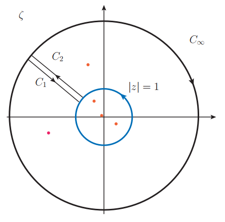
Figure 2: The contours for Eq.(3.4) and singularities (red dot) of the function $\mathcal{N}_{\zeta}S(\rho_{A}(\zeta))$.

Note that the function $\mathcal{N}_{\zeta}S(\rho_{A}(\zeta))$ is expected to exhibit singularities on the $\zeta$ plane. As $\zeta\to 0$, $\rho(\zeta)\to\frac{|\phi\rangle\langle\psi|}{\langle\psi|\psi\rangle}$, yet $\mathcal{N}_{\zeta}\to\frac{1}{\zeta^{3}}\frac{\langle\psi|\phi\rangle}{\langle\phi|\psi\rangle}$. Consequently, $\mathcal{N}_{\zeta}S(\rho_{A}(\zeta))$ is guaranteed to have at least one singularity at $\zeta=0$. The exact singularities of $S(\rho_{A}(\zeta))$ depends on states that we consider. In general, assume there exists singularities as shown in Fig.2. By residue theorem we can express PE as the residue summations over the $\zeta$ plane,

$$S(\mathcal{T}_{A}^{\psi|\phi})=\sum_{i,\zeta\ \text{plane}}\text{Res}\left[\mathcal{N}_{\zeta}S(\rho_{A}(\zeta)),a_{i}\right].$$ (44)

This formula is valuable for evaluating the PE. However, our primary aim is to establish a connection between the PE $S(\mathcal{T}_{A}^{\psi|\phi})$ and the EE of $\rho_{A}(\theta)$. Therefore, one may use for the contours depicted in Fig.2, as they facilitate this investigation. Again, by using residue theorem we have

$$\frac{1}{2\pi i}\oint_{C_{\infty}}d\zeta\mathcal{N}_{\zeta}S(\rho_{A}(\zeta))+\frac{1}{2\pi i}\oint_{C_{1}}d\zeta\mathcal{N}_{\zeta}S(\rho_{A}(\zeta))+\frac{1}{2\pi i}\oint_{C_{2}}d\zeta\mathcal{N}_{\zeta}S(\rho_{A}(\zeta))$$

$$+\frac{1}{2\pi i}\oint_{|\zeta|=1}d\zeta\mathcal{N}_{\zeta}S(\rho_{A}(\zeta))=-\sum_{i,|\zeta|>1}\text{Res}\left[\mathcal{N}_{\zeta}S(\rho_{A}(\zeta)),a_{i}\right],$$ (45)

where $C_{1}$ and $C_{2}$ are two arbitrarily chosen paths that do not pass through any singularities. The contributions to the integral from $C_{1}$ and $C_{2}$ cancel each other out provided they are sufficiently close. By using (43) we find

$$S(\mathcal{T}_{A}^{\psi|\phi})=\frac{1}{2\pi i}\oint_{|\zeta|=1}d\zeta\mathcal{N}_{\zeta}S(\rho_{A}(\zeta))+\sum_{i,|\zeta|>1}\text{Res}\left[\mathcal{N}_{\zeta}S(\rho_{A}(\zeta)),a_{i}\right].$$ (46)

Comparing with formula (39), we observe additional contributions from the summation of residues in the region $|\zeta|>1$. In the special case that there exists no singularities in $|\zeta|>1$. The formula (46) would reduce to (39). In the following sections, we will consider some examples that demonstrate the correctness of the sum rule formula (46) for general cases.

Before we move one let us comment the formula that we derived in section.3.3. In that approach there are no additional terms of the residues contributions (46). In the approach outlined in Section 3.3, we make two assumptions. First, we assume that the order of integration and limit can be interchanged in Eq.(3.3). Second, we assume that the limit $\lim_{z\to-\infty}G[z^{\prime},\rho(\theta)]$ with $z^{\prime}=ze^{-i\theta}\mathcal{N}_{\theta}$ exists and equals $S(\rho_{A}(\theta))$. The function $G[z^{\prime},\rho(\theta)]$ has a branch cut on $[1,\infty]$. When taking the limit $z\to-\infty$, we need to avoid the branch cut. However, $z^{\prime}=ze^{-i\theta}\mathcal{N}_{\theta}$ may encounter the branch cut for certain values of $\theta$, which may pose a problem. Currently, we do not have a solution for this issue. Nonetheless, the derivation of (46) in this section remains valid.

4 Examples

To check the sum rule formula for PE we will consider some examples in this section.

4.1 Qubit examples

Assume the basis of two qubits system are $|00\rangle$, $|01\rangle$, $|10\rangle$ and $|11\rangle$. Define two pure states

$$|\phi\rangle=\frac{1}{\sqrt{|\alpha_{\phi}|^{2}+|\beta_{\phi}|^{2}}}(\alpha_{\phi}|00\rangle+\beta_{\phi}|11\rangle),$$

$$|\psi\rangle=\frac{1}{\sqrt{|\alpha_{\psi}|^{2}+|\beta_{\psi}|^{2}}}(\alpha_{\psi}|00\rangle+\beta_{\psi}|11\rangle),$$ (47)

where $\alpha_{\phi}$, $\alpha_{\psi}$, $\beta_{\phi}$ and $\beta_{\psi}$ are arbitrary constants. The reduced density matrix of the superposition state $|\xi(\theta)\rangle=\mathcal{N}(\theta)(|\phi\rangle+e^{i\theta}|\psi\rangle)$ is diagonal,

$$\rho_{A}(\theta)=\begin{pmatrix}\lambda_{1}&0\\ 0&\lambda_{2}\end{pmatrix},$$ (48)

with

$$\lambda_{1}=[\mathcal{N}(\theta)]^{2}\Big{|}\frac{\alpha_{\phi}}{\sqrt{|\alpha_{\phi}|^{2}+|\beta_{\phi}|^{2}}}+\frac{\alpha_{\psi}\mathrm{e}^{i\theta}}{\sqrt{|\alpha_{\psi}|^{2}+|\beta_{\psi}|^{2}}}\Big{|}^{2},$$

$$\lambda_{2}=[\mathcal{N}(\theta)]^{2}\Big{|}\frac{\beta_{\phi}}{\sqrt{|\alpha_{\phi}|^{2}+|\beta_{\phi}|^{2}}}+\frac{\beta_{\psi}\mathrm{e}^{i\theta}}{\sqrt{|\alpha_{\psi}|^{2}+|\beta_{\psi}|^{2}}}\Big{|}^{2},$$

where

$$[\mathcal{N}(\theta)]^{-2}=\Big{|}\frac{\alpha_{\phi}}{\sqrt{|\alpha_{\phi}|^{2}+|\beta_{\phi}|^{2}}}+\frac{\alpha_{\psi}\mathrm{e}^{i\theta}}{\sqrt{|\alpha_{\psi}|^{2}+|\beta_{\psi}|^{2}}}\Big{|}^{2}$$

$$\phantom{[\mathcal{N}(\theta)]^{-2}=}+\Big{|}\frac{\beta_{\phi}}{\sqrt{|\alpha_{\phi}|^{2}+|\beta_{\phi}|^{2}}}+\frac{\beta_{\psi}\mathrm{e}^{i\theta}}{\sqrt{|\alpha_{\psi}|^{2}+|\beta_{\psi}|^{2}}}\Big{|}^{2}.$$ (49)

The reduced transition matrix $\mathcal{T}_{A}^{\psi|\phi}$ is also diagonal, which is

$$\mathcal{T}_{A}^{\psi|\phi}=\left(\begin{array}[]{cc}t_{1}&0\\ 0&t_{2}\\ \end{array}\right),$$ (52)

with

$$t_{1}=\frac{\alpha^{*}_{\phi}\alpha_{\psi}}{\alpha^{*}_{\phi}\alpha_{\psi}+\beta^{*}_{\phi}\beta_{\psi}},~{}~{}t_{2}=\frac{\beta^{*}_{\phi}\beta_{\psi}}{\alpha^{*}_{\phi}\alpha_{\psi}+\beta^{*}_{\phi}\beta_{\psi}}.$$

Here we consider $\alpha_{\phi}=\alpha_{\psi}=\beta_{\phi}=1$ and $\beta_{\psi}=e^{i\gamma}$. Assume $|\gamma|\ll 1$, thus we could expand the $S(\rho_{A}(\theta))$ as well as $S(\mathcal{T}_{A}^{\psi|\phi})$ with respect to parameter $\gamma$. With some calculation we have

$$S(\mathcal{T}_{A}^{\psi|\phi})=\log(2)+\frac{\gamma^{2}}{8}+\frac{\gamma^{4}}{64}+O\left(\gamma^{5}\right),$$ (53)

and

$$\mathcal{N}_{\zeta}S(\rho(\zeta))=\frac{(\zeta+1)^{2}\log(2)}{\zeta^{3}}-\frac{i\gamma(\zeta+1)\log(2)}{\zeta^{3}}+\frac{\gamma^{2}\left(\zeta^{2}-2\zeta+1-4\log(2)\right)}{8\zeta^{3}}$$

$$\phantom{\mathcal{N}_{\zeta}S(\rho(\zeta))}-\frac{i\gamma^{3}((2\log(2)-3)\zeta+3-4\log(2))}{24\zeta^{3}}$$

$$\phantom{\mathcal{N}_{\zeta}S(\rho(\zeta))}+\frac{\gamma^{4}\left(3\zeta^{4}+4\zeta^{3}+(10\log(2)-2)\zeta^{2}+4(4\log(2)-5)\zeta-9+10\log(2)\right)}{192\zeta^{3}(\zeta+1)^{2}}+O(\gamma^{5}).$$

One could evaluate the residues of the above formula in the unit circle,

$$\sum_{i,|\zeta|\leq 1}\text{Res}\left[\mathcal{N}_{\zeta}S(\rho_{A}(\zeta)),a_{i}\right]=\log(2)+\frac{\gamma^{2}}{8}+\frac{\gamma^{4}}{64}+O\left(\gamma^{5}\right).$$ (54)

The sum rule formula (37) is correct for this case. One can compute the outcomes up to any desired order of $O(\gamma)$ and demonstrate the validity of the sum rule. Note that the sum rule for PE (28) derived in [37] is only valid up to the order of $O(\gamma^{2})$.

4.2 Perturbation state

Let us consider the two states $|\psi\rangle$ and $|\phi\rangle=\mathcal{N}_{\phi}(|\psi\rangle+\epsilon|\psi^{\prime}\rangle)$, where $\mathcal{N}_{\phi}=1-\frac{1}{2}(\epsilon\langle\psi|\psi^{\prime}\rangle+\epsilon^{*}\langle\psi^{\prime}|\psi\rangle$+O($\epsilon^{2}$). We have

$$\langle\phi|\psi\rangle=1+\frac{1}{2}\epsilon^{*}\langle\psi^{\prime}|\psi\rangle-\frac{1}{2}\epsilon\langle\psi|\psi^{\prime}\rangle+O(\epsilon^{2}).$$ (55)

The reduced transition matrix is given by

$$\mathcal{T}_{A}^{\psi|\phi}=\rho_{A}^{\psi}-\epsilon^{*}\langle\psi^{\prime}|\psi\rangle\rho_{A}^{\psi}+\epsilon^{*}\mathcal{T}_{A}^{\psi|\psi^{\prime}}+O(\epsilon^{2}).$$ (56)

The superposition state is

$$|\xi(\theta)\rangle=\mathcal{N}(\theta)\left[(1+e^{i\theta})|\psi\rangle-\frac{1}{2}(\epsilon\langle\psi|\psi^{\prime}\rangle+\epsilon^{*}\langle\psi^{\prime}|\psi\rangle)|\psi\rangle-\epsilon|\psi^{\prime}\rangle\right]+O(\epsilon^{2}),$$ (57)

where the normalization satisfies

$$\mathcal{N}(\theta)^{2}|1+e^{i\theta}|^{2}=1+\frac{1}{2}\frac{1}{1+e^{i\theta}}(\epsilon\langle\psi|\psi^{\prime}\rangle+\epsilon^{*}\langle\psi^{\prime}|\psi\rangle)+\frac{1}{2}\frac{1}{1+e^{-i\theta}}(\epsilon\langle\psi|\psi^{\prime}\rangle+\epsilon^{*}\langle\psi^{\prime}|\psi\rangle)$$

$$\phantom{\mathcal{N}(\theta)^{2}|1+e^{i\theta}|^{2}=}+\epsilon^{*}\frac{1}{1+e^{-i\theta}}\langle\psi^{\prime}|\psi\rangle+\epsilon\frac{1}{1+e^{i\theta}}\langle\psi|\psi^{\prime}\rangle+O(\epsilon^{2}).$$ (58)

The reduced density matrix $\rho_{A}(\theta)$ is given by

$$\rho_{A}(\theta)=\rho_{A}^{\psi}+\epsilon^{*}\frac{1}{1+e^{-i\theta}}\langle\psi^{\prime}|\psi\rangle\rho_{A}^{\psi}-\epsilon^{*}\frac{1}{1+e^{-i\theta}}\mathcal{T}_{A}^{\psi|\psi^{\prime}}$$

$$\phantom{\rho_{A}(\theta)=\rho_{A}^{\psi}}+\epsilon\frac{1}{1+e^{i\theta}}\langle\psi|\psi^{\prime}\rangle\rho_{A}^{\psi}-\epsilon\frac{1}{1+e^{i\theta}}\mathcal{T}_{A}^{\psi^{\prime}|\psi}+O(\epsilon^{2}).$$ (59)

It would be straightforward to verify the correctness of the operator sum rule (8) at the leading order of $O(\epsilon)$. In [37] we have shown actually the sum rule (28) is correct at the leading order of $O(\epsilon)$, but it can not be applicable at the order of $O(\epsilon^{2})$. One could evaluate the EE and PE at the leading order of $O(\epsilon)$ and check the sum rule for PE (37). Moreover, we would like to show it is also correct for the the order of $O(\epsilon^{2})$.

4.2.1 Perturbation calculation of EE and PE

At the leading order of $O(\epsilon)$ both EE and PE satisfy the first-law like relation, we have

$$\delta S^{(1)}(\mathcal{T}_{A}^{\psi|\phi})=-\epsilon^{*}\langle\psi^{\prime}|\psi\rangle\langle\psi|H_{A}^{\psi}|\psi\rangle+\epsilon^{*}\langle\psi^{\prime}|H_{A}^{\psi}|\psi\rangle,$$ (60)

and

$$\delta S^{(1)}(\rho(\theta))=\epsilon^{*}\frac{1}{1+e^{-i\theta}}\langle\psi^{\prime}|\psi\rangle\langle\psi|H_{A}^{\psi}|\psi\rangle-\epsilon^{*}\frac{1}{1+e^{-i\theta}}\langle\psi^{\prime}|H_{A}^{\psi}|\psi\rangle$$

$$\phantom{\delta S^{(1)}(\rho(\theta))}+\epsilon\frac{1}{1+e^{i\theta}}\langle\psi|\psi^{\prime}\rangle\langle\psi|H_{A}^{\psi}|\psi\rangle-\epsilon\frac{1}{1+e^{i\theta}}\langle\psi^{\prime}|H_{A}^{\psi}|\psi\rangle,$$ (61)

where $H_{A}^{\psi}:=-\log\rho_{A}^{\psi}$ is the modular Hamiltonian for the state $\rho_{A}^{\psi}$.

For an operator $M$ with $trM=1$ we have the identity

$$-\log M=\int_{0}^{\infty}d\beta\left(\frac{1}{\beta+M}-\frac{1}{\beta+1}\right).$$ (62)

For our purposes, $M$ would stand for the reduced density matrix $\rho_{A}(\theta)$ (4.2) or transition matrix $\mathcal{T}_{A}^{\psi|\phi}$ (56). We also have the entropy formula

$$S(M)=-\textrm{tr}M\log M=\int_{0}^{\infty}d\beta\left(trM\frac{1}{\beta+M}-\frac{1}{\beta+1}\right).$$ (63)

We want to consider the second order variation of $S$ under the perturbation $M+\delta M$ with $tr\delta M=0$. The result is

$$\delta S^{(2)}(M)=-\int_{0}^{\infty}d\beta\beta\textrm{tr}\left(\frac{1}{(\beta+M)^{2}}\delta M\frac{1}{\beta+M}\delta M\right),$$ (64)

see Appendix.A for details. Now the result can be used for the operator $\mathcal{T}_{A}^{\psi|\phi}$ (56) and $\rho(\theta)$ (4.2). There is a subtle point. Typically, the spectra of the reduced transition matrix are complex. If $\mathcal{T}_{A}^{\psi|\phi}$ exhibits negative spectra, the expression above might become undefined. Hence, it’s preferable to assume that $\mathcal{T}_{A}^{\psi|\phi}$ does not possess negative spectra. We have

$$\delta S^{(2)}(\mathcal{T}_{A}^{\psi|\phi})=-(\epsilon^{*})^{2}\langle\psi^{\prime}|\psi\rangle^{2}\int_{0}^{\infty}d\beta\beta\textrm{tr}\left(\frac{1}{(\beta+\rho_{A}^{\psi})^{2}}\rho_{A}^{\psi}\frac{1}{\beta+\rho_{A}^{\psi}}\rho_{A}^{\psi}\right)$$

$$\phantom{\delta S^{(2)}(\mathcal{T}_{A}^{\psi|\phi})=}+(\epsilon^{*})^{2}\langle\psi^{\prime}|\psi\rangle\int_{0}^{\infty}d\beta\beta\textrm{tr}\left(\frac{1}{(\beta+\rho_{A}^{\psi})^{2}}\rho_{A}^{\psi}\frac{1}{\beta+\rho_{A}^{\psi}}\mathcal{T}^{\psi|\psi^{\prime}}\right)$$

$$\phantom{\delta S^{(2)}(\mathcal{T}_{A}^{\psi|\phi})=}+(\epsilon^{*})^{2}\langle\psi^{\prime}|\psi\rangle\int_{0}^{\infty}d\beta\beta\textrm{tr}\left(\frac{1}{(\beta+\rho_{A}^{\psi})^{2}}\mathcal{T}^{\psi|\psi^{\prime}}\frac{1}{\beta+\rho_{A}^{\psi}}\rho_{A}^{\psi}\right)$$

$$\phantom{\delta S^{(2)}(\mathcal{T}_{A}^{\psi|\phi})=}-(\epsilon^{*})^{2}\int_{0}^{\infty}d\beta\beta\textrm{tr}\left(\frac{1}{(\beta+\rho_{A}^{\psi})^{2}}\mathcal{T}^{\psi|\psi^{\prime}}\frac{1}{\beta+\rho_{A}^{\psi}}\mathcal{T}^{\psi|\psi^{\prime}}\right),$$ (65)

and

$$\delta S^{(2)}(\rho_{A}(\theta))=-(\epsilon^{*})^{2}\frac{\langle\psi^{\prime}|\psi\rangle^{2}}{(1+e^{-i\theta})^{2}}\int_{0}^{\infty}d\beta\beta\textrm{tr}\left(\frac{1}{(\beta+\rho_{A}^{\psi})^{2}}\rho_{A}^{\psi}\frac{1}{\beta+\rho_{A}^{\psi}}\rho_{A}^{\psi}\right)$$

$$\phantom{\delta S^{(2)}(\rho_{A}(\theta))=}+(\epsilon^{*})^{2}\frac{\langle\psi^{\prime}|\psi\rangle}{(1+e^{-i\theta})^{2}}\int_{0}^{\infty}d\beta\beta\textrm{tr}\left(\frac{1}{(\beta+\rho_{A}^{\psi})^{2}}\rho_{A}^{\psi}\frac{1}{\beta+\rho_{A}^{\psi}}\mathcal{T}^{\psi|\psi^{\prime}}\right)$$

$$\phantom{\delta S^{(2)}(\rho_{A}(\theta))=}+(\epsilon^{*})^{2}\frac{\langle\psi^{\prime}|\psi\rangle}{(1+e^{-i\theta})^{2}}\int_{0}^{\infty}d\beta\beta\textrm{tr}\left(\frac{1}{(\beta+\rho_{A}^{\psi})^{2}}\mathcal{T}^{\psi|\psi^{\prime}}\frac{1}{\beta+\rho_{A}^{\psi}}\rho_{A}^{\psi}\right)$$

$$\phantom{\delta S^{(2)}(\rho_{A}(\theta))=}-(\epsilon^{*})^{2}\frac{1}{(1+e^{-i\theta})^{2}}\int_{0}^{\infty}d\beta\beta\textrm{tr}\left(\frac{1}{(\beta+\rho_{A}^{\psi})^{2}}\mathcal{T}^{\psi|\psi^{\prime}}\frac{1}{\beta+\rho_{A}^{\psi}}\mathcal{T}^{\psi|\psi^{\prime}}\right)$$

$$\phantom{\delta S^{(2)}(\rho_{A}(\theta))=}+h.c.,$$ (66)

4.2.2 Sum rule for perturbation state

Now using the results (4.2.1) (4.2.1), one could check the sum rule (37) or (39). By definition we have

$$\mathcal{N}_{\theta}=(2+e^{i\theta}\langle\phi|\psi\rangle+e^{-i\theta}\langle\psi|\phi\rangle)\langle\phi|\psi\rangle^{-1}$$

$$\phantom{\mathcal{N}_{\theta}}=2+e^{i\theta}+e^{-i\theta}-\epsilon^{*}\langle\psi^{\prime}|\psi\rangle(1+e^{-i\theta})+\epsilon\langle\psi|\psi^{\prime}\rangle(1+e^{-i\theta})+O(\epsilon^{2}).$$

At the leading order of $O(\epsilon)$ by using (60) (4.2.1) and (4.2.2) we have

$$\frac{1}{2\pi}\int_{-\pi}^{\pi}d\theta e^{-i\theta}(2+e^{i\theta}+e^{-i\theta})\delta S^{(1)}(\rho(\theta))$$

$$=\frac{1}{2\pi}\int_{-\pi}^{\pi}d\theta(1+e^{-i\theta})^{2}\delta S^{(1)}(\rho(\theta))=\delta S^{(1)}(\mathcal{T}_{A}^{\psi|\phi}).$$ (67)

This result demonstrates the validity of the sum rule (37) at the leading order of $O(\epsilon)$. To investigate the order of $O(\epsilon^{2})$, we must assess two terms. The first involves the multiplication of the $O(\epsilon)$ component of $\mathcal{N}_{\theta}$ (4.2.2) with $\delta S^{(1)}$, that is

$$\frac{1}{2\pi}\int_{-\pi}^{\pi}d\theta e^{-i\theta}(-\epsilon^{*}\langle\psi^{\prime}|\psi\rangle(1+e^{-i\theta})+\epsilon\langle\psi|\psi^{\prime}\rangle(1+e^{-i\theta}))\delta S^{(1)}(\rho(\theta)),$$ (68)

which is vanishing. The other term is

$$\frac{1}{2\pi}\int_{-\pi}^{\pi}d\theta e^{-i\theta}(2+e^{i\theta}+e^{-i\theta})\delta S^{(2)}(\rho(\theta))=\delta S^{(2)}(\mathcal{T}_{A}^{\psi|\phi}),$$ (69)

which can be confirmed through straightforward calculations. Thus, we have established the validity of the sum rule for the PE (37) for the perturbed state up to the order of $O(\epsilon^{2})$. Furthermore, one could extend these calculations to demonstrate its correctness for any order of perturbation.

4.3 Short interval expansion

Consider an interval $A$ with length $\ell$ in 2-dimensional CFT . One could evaluate the pseudoentropy and EE by using operator product expansion (OPE) of twist operator [53]-[57]. For the reduced density matrix $\rho_{A}$ we have the expansion

$$S_{A}(\rho_{A})=\frac{c}{3}\log\frac{\ell}{\epsilon}+\sum_{m=1}^{n}\sum_{\mu\mathcal{X}_{1},...,\mathcal{X}_{m}}\ell^{\Delta_{\mu\mathcal{X}_{1}}+...+\Delta_{\mathcal{X}_{m}}}a_{\mu\mathcal{X}_{1}...\mathcal{X}_{m}}tr(\rho_{A}\mu\mathcal{X}_{1})...tr(\rho_{A}\mathcal{X}_{m}),$$ (70)

where $\mathcal{X}_{i}$ ($i=1,...,m$) are the quasi-primary operators for the OPE of twist operator, $\Delta_{\mathcal{X}_{i}}$ are their conformal dimension, $h_{\sigma}$ is the conformal weight of twist operator, $a_{\mu\mathcal{X}_{1}...\mathcal{X}_{m}}$ are the constant coefficients that are independent with $\rho_{A}$. For the transition matrix $\mathcal{T}_{A}^{\psi|\phi}$ we also have the similar expansion

$$S_{A}(\mathcal{T}_{A}^{\psi|\phi})=\frac{c}{3}\log\frac{\ell}{\epsilon}+\sum_{m=1}^{n}\sum_{\mathcal{X}_{1},...,\mathcal{X}_{m}}\ell^{\Delta_{\mu\mathcal{X}_{1}}+...+\Delta_{\mathcal{X}_{m}}}a_{\mu\mathcal{X}_{1}...\mathcal{X}_{m}}tr(\mathcal{T}_{A}^{\psi|\phi}\mu\mathcal{X}_{1})...tr(\mathcal{T}_{A}^{\psi|\phi}\mathcal{X}_{m}).$$ (71)

Define the function $F_{m}(\theta):=tr(\rho_{A}(\theta)\mu\mathcal{X}_{1})...tr(\rho(\theta)_{A}\mathcal{X}_{m})$, which can be expanded as

$$F_{m}(\theta)=\mathcal{N}(\theta)^{2m}\prod_{i=1}^{m}\left(\langle\phi|\mathcal{X}_{i}|\phi\rangle+e^{-i\theta}\langle\psi|\mathcal{X}_{i}|\phi\rangle+e^{i\theta}\langle\phi|\mathcal{X}_{i}|\psi\rangle+\langle\psi|\mathcal{X}_{i}|\psi\rangle\right),$$ (72)

Note that the coefficients $a_{\mu\mathcal{X}_{1}...\mathcal{X}_{m}}$ are same for the PE and EE. To check the sum rule we only need to consider the following integral,

$$\frac{1}{2\pi}\int_{-\pi}^{\pi}d\theta e^{-i\theta}\mathcal{N}_{\theta}F_{m}(\theta)$$

$$=\frac{1}{2\pi}\int_{-\pi}^{\pi}d\theta e^{-i\theta}\frac{\prod_{i=1}^{m}\left(\langle\phi|\mathcal{X}_{i}|\phi\rangle+e^{-i\theta}\langle\psi|\mathcal{X}_{i}|\phi\rangle+e^{i\theta}\langle\phi|\mathcal{X}_{i}|\psi\rangle+\langle\psi|\mathcal{X}_{i}|\psi\rangle\right)}{\langle\phi|\psi\rangle\left(2+e^{i\theta}\langle\phi|\psi\rangle+e^{-i\theta}\langle\psi|\phi\rangle\right)^{m-1}}$$

With $\zeta=e^{i\theta}$ we have

$$\frac{1}{2\pi}\int_{-\pi}^{\pi}d\theta e^{-i\theta}\mathcal{N}_{\theta}F_{m}(\theta)=\frac{1}{2\pi i}\oint_{|\zeta|=1}d\zeta\mathcal{F}_{m}(\zeta),$$

with

$$\mathcal{F}_{m}(\zeta):=\frac{1}{\zeta^{3}}\frac{\prod_{i=1}^{m}\left(\zeta\langle\phi|\mathcal{X}_{i}|\phi\rangle+\langle\psi|\mathcal{X}_{i}|\phi\rangle+\zeta^{2}\langle\phi|\mathcal{X}_{i}|\psi\rangle+\zeta\langle\psi|\mathcal{X}_{i}|\psi\rangle\right)}{\langle\phi|\psi\rangle\left(2\zeta+\zeta^{2}\langle\phi|\psi\rangle+\langle\psi|\phi\rangle\right)^{m-1}}.$$ (73)

To compute the integration, we must identify the singularities of the integrand within the unit circle $|\zeta|\leq 1$. Utilizing the Cauchy–Schwarz inequality, we have $|\langle\phi|\psi\rangle|\leq 1$. For $m\geq 1$, within the unit circle, there are two singularities at $\zeta=0$ and $\zeta=\frac{-1+\sqrt{1-|\langle\phi|\psi\rangle|^{2}}}{\langle\phi|\psi\rangle}$. Note that the integrand also has a singularity at $\zeta=\frac{-1-\sqrt{1-|\langle\phi|\psi\rangle|^{2}}}{\langle\phi|\psi\rangle}$.

4.4 Results for $m=1,2$

Now, we aim to evaluate the integral (4.3). Firstly, let’s consider $m=1$. In this case, $\zeta=0$ is the only singularity. The result is

$$\frac{1}{2\pi}\int_{-\pi}^{\pi}d\theta e^{-i\theta}\mathcal{N}_{\theta}F_{1}(\theta)=\frac{\langle\phi|\mathcal{X}_{1}|\psi\rangle}{\langle\phi|\psi\rangle},$$ (74)

which is consistent with the sum rule (37). Then, let us consider $m=2$. As noted above there are two singularities $\zeta_{0}=0$ and $\zeta_{1}=\frac{-1+\sqrt{1-|\langle\phi|\psi\rangle|^{2}}}{\langle\phi|\psi\rangle}$ within the unit circle $|\zeta|\leq 1$, while the singularity $\zeta_{2}=\frac{-1-\sqrt{1-|\langle\phi|\psi\rangle|^{2}}}{\langle\phi|\psi\rangle}$ is in the region $|\zeta|\geq 1$. Thus we have

$$\frac{1}{2\pi}\int_{-\pi}^{\pi}d\theta e^{-i\theta}\mathcal{N}_{\theta}F_{2}(\theta)=\sum_{j=0,1}\text{Res}[\mathcal{F}_{2}(\zeta),\zeta_{j}]$$

With some calculations we find

$$\frac{1}{2\pi}\int_{-\pi}^{\pi}d\theta e^{-i\theta}\mathcal{N}_{\theta}F_{2}(\theta)=-\frac{1}{\zeta_{1}^{3}\left(\zeta_{1}-\zeta_{2}\right)\langle\phi|\psi\rangle}\Big{[}\left\langle\psi\left|\mathcal{X}_{1}\right|\phi\right\rangle\left\langle\psi\left|\mathcal{X}_{2}\right|\phi\right\rangle$$

$$+\zeta_{1}\left(\left\langle\phi\left|\mathcal{X}_{1}\right|\phi\right\rangle\left\langle\psi\left|\mathcal{X}_{2}\right|\phi\right\rangle+\left\langle\psi\left|\mathcal{X}_{1}\right|\psi\right\rangle\left\langle\psi\left|\mathcal{X}_{2}\right|\phi\right\rangle+\left\langle\psi\left|\mathcal{X}_{1}\right|\phi\right\rangle\left(\left\langle\psi\left|\mathcal{X}_{2}\right|\psi\right\rangle+\left\langle\phi\left|\mathcal{X}_{2}\right|\phi\right\rangle\right)\right)$$

$$\zeta_{1}^{2}\big{(}\left\langle\phi\left|\mathcal{X}_{2}\right|\psi\right\rangle\left\langle\psi\left|\mathcal{X}_{1}\right|\phi\right\rangle+\left\langle\phi\left|\mathcal{X}_{1}\right|\psi\right\rangle\left\langle\psi\left|\mathcal{X}_{2}\right|\phi\right\rangle+\left\langle\phi\left|\mathcal{X}_{1}\right|\phi\right\rangle\left(\left\langle\psi\left|\mathcal{X}_{2}\right|\psi\right\rangle+\left\langle\phi\left|\mathcal{X}_{2}\right|\phi\right\rangle\right)$$

$$+\left\langle\psi\left|\mathcal{X}_{1}\right|\psi\right\rangle\left(\left\langle\psi\left|\mathcal{X}_{2}\right|\psi\right\rangle+\left\langle\phi\left|\mathcal{X}_{2}\right|\phi\right\rangle\right)\big{)}+\zeta_{1}^{3}\big{(}(\left\langle\phi\left|\mathcal{X}_{2}\right|\psi\right\rangle\left(\left\langle\phi\left|\mathcal{X}_{1}\right|\phi\right\rangle+\left\langle\psi\left|\mathcal{X}_{1}\right|\psi\right\rangle\right)$$

$$+\left\langle\phi\left|\mathcal{X}_{1}\right|\psi\right\rangle\left(\left\langle\phi\left|\mathcal{X}_{2}\right|\phi\right\rangle+\left\langle\psi\left|\mathcal{X}_{2}\right|\psi\right\rangle\right))+\left\langle\phi\left|\mathcal{X}_{1}\right|\psi\right\rangle\left\langle\phi\left|\mathcal{X}_{2}\right|\psi\right\rangle\zeta_{2}\big{)}\Big{]}.$$ (75)

This result indicates that the sum rule (37) is not valid in this instance. However, formula (46) stands as the correct one. We can calculate the contributions of the singularity at point $\zeta_{2}$, and it is straightforward to verify that

$$\frac{1}{2\pi}\int_{-\pi}^{\pi}d\theta e^{-i\theta}\mathcal{N}_{\theta}F_{2}(\theta)+\text{Res}[\mathcal{F}_{2}(\zeta),\zeta_{2}]=\frac{\langle\phi|\mathcal{X}_{1}|\psi\rangle\langle\phi|\mathcal{X}_{2}|\psi\rangle}{\langle\phi|\psi\rangle^{2}},$$ (76)

the right-hand of which yields the anticipated outcome for the short interval expansion of PE.

4.5 Results for arbitrary $m$

Indeed, one could verify the outcomes for $m>2$ through direct calculations. Here we show that one could obtain the results for any $m$ by the property of the function $\mathcal{F}_{m}(\zeta)$. The argument here is analogous to the general proof presented in section.3.4. In the limit $\zeta\to\infty$ we find

$$\lim_{\zeta\to\infty}\mathcal{F}_{m}(\zeta)\to\frac{1}{\zeta}\frac{\prod_{i=1}^{m}\langle\phi|\mathcal{X}_{i}|\psi\rangle}{\langle\phi|\psi\rangle^{m}}.$$ (77)

Note that the coefficient of $\frac{1}{\zeta}$ in the above formula precisely represents the term for evaluating PE. Therefore, this term can be isolated by integrating along the circle $C_{\infty}$ at infinity, as illustrated in Fig. 2. For all functions $\mathcal{F}m(\zeta)$, there exist three singularities ${\zeta_{0},\zeta_{1},\zeta_{2}}$, as discussed in previous sections. Hence, it is feasible to rewrite the integral along the circle $C\infty$ as a summation of residues on the $\zeta$ plane.

$$\frac{\prod_{i=1}^{m}\langle\phi|\mathcal{X}_{i}|\psi\rangle}{\langle\phi|\psi\rangle^{m}}=\sum_{i,\zeta\ \text{plane}}\text{Res}\left[\mathcal{F}_{m},\zeta_{i}\right].$$ (78)

While the residues summations for $\zeta_{0}$ and $\zeta_{1}$ can be rewritten as integral on the unit circle $|\zeta|=1$. As a result we have

$$\frac{1}{2\pi}\int_{-\pi}^{\pi}d\theta e^{-i\theta}\mathcal{N}_{\theta}F_{m}(\theta)+\text{Res}[\mathcal{F}_{m}(\zeta),\zeta_{2}]=\frac{\prod_{i=1}^{m}\langle\phi|\mathcal{X}_{i}|\psi\rangle}{\langle\phi|\psi\rangle^{m}}.$$ (79)

By employing the above formula, one can demonstrate the sum rule for PE (46) in the short interval expansion.

5 Applications

5.1 Holographic dual of transition matrix

The transition matrix is typically non-Hermitian, resulting in its spectra, as well as pseudo-Rényi entropy and PE, being complex. It is anticipated that there exists a subset of transition matrices whose spectra are positive. For these states, both pseudo-Rényi entropy and PE are positive. In the context of AdS/CFT, this subset of transition matrices may have a bulk dual. Given that the calculation method for pseudo-Rényi entropy and PE in QFTs closely parallels that of Rényi entropy and EE, it is reasonable to anticipate that if a given transition matrix $\mathcal{T}^{\psi|\phi}$ possesses a bulk geometric dual, then pseudo-Rényi entropy and PE may also have corresponding bulk geometric interpretations. For PE, its bulk dual is similarly described by the RT formula.

In [19], the authors utilize the concept of pseudo-Hermiticity to classify transition matrices. They particularly focus on a class of transition matrices $\mathcal{T}^{\psi|\phi}$ for which $|\phi\rangle=\eta|\psi\rangle$, with $\eta$ being a Hermitian and invertible operator. In such cases where the transition matrix exhibits pseudo-Hermitian properties, it possesses certain distinctive characteristics. Moreover, if $\eta$ can be expressed as an integration or summation of local operators, then for any subsystem $A$, $\eta$ can be decomposed into $\eta_{A}\otimes\eta_{\bar{A}}$.

It is further demonstrated in [19] that if both $\eta_{A}$ and $\eta_{\bar{A}}$ are either positive or negative operators, the reduced transition matrix $\mathcal{T}_{A}^{\psi|\phi}$ should exhibit positive spectra. Consequently, the pseudo-Rényi entropy and PE also yield positive values. Transition matrices of this kind may potentially possess a bulk geometric dual.

The sum rules that we explored in this paper may have interesting geometric explanation if the transition matrix can be dual to a bulk geometry. In the traditional treatment the bulk geometry is considered to be associated with boundary state with a given density matrix. It is generally expected the theory can be dual to gravity should be a gapped large-N QFTs[58][59] with bulk Newton constant $G\sim 1/N^{2}$. The semi-classical limit $G\to 0$ corresponds to the large $N$ limit in the dual QFT. If a state $|\Psi\rangle$ has a bulk geometric dual, the connected 2-point correlation functions of any single trace operator $\mathcal{O}_{i}$ should satisfy the following relation

$$\langle\Psi|\mathcal{O}_{i}\mathcal{O}_{j}|\Psi\rangle-\langle\Psi|\mathcal{O}_{i}|\Psi\rangle\langle\Psi|\mathcal{O}_{j}|\Psi\rangle\sim O(N^{2}).$$ (80)

Let us assume the state $\rho(\theta):=|\xi(\theta)\rangle\langle\xi(\theta)|$ can be dual to bulk geometry. Thus the single trace operators satisfy the relation (80) for $|\xi(\theta)\rangle$. Now using the sum rule for the correlators (10), we have

$$\frac{\langle\phi|\mathcal{O}_{i}\mathcal{O}_{j}|\psi\rangle-\langle\phi|\mathcal{O}_{i}|\psi\rangle\langle\phi|\mathcal{O}_{j}|\psi\rangle}{\langle\phi|\psi\rangle^{2}}$$

$$=\frac{1}{2\pi}\int_{-\pi}^{\pi}d\theta e^{-in\theta}\mathcal{N}_{\theta}^{n}\left(\langle\xi(\theta)|\mathcal{O}_{i}\mathcal{O}_{j}|\xi(\theta)\rangle-\langle\xi(\theta)|\mathcal{O}_{i}|\xi(\theta)\rangle\langle\xi(\theta)|\mathcal{O}_{j}|\xi(\theta)\rangle\right).$$

Notice that the term inside the brackets scales as $O(N^{2})$. Consequently, the left-hand side of the equation above should also scale as $O(N^{2})$. This reasoning extends to $n$-point correlation functions. The sum rule (10) ensures that both the superposition state $\rho(\theta)$ and the transition matrix $\mathcal{T}^{\psi|\phi}$ exhibit the same scaling behavior in the large $N$ limit. Therefore, if the state $\rho(\theta)$ can be effectively described by a bulk geometry, it suggests the possibility that the transition matrix $\mathcal{T}^{\psi|\phi}$ is also dual to some bulk geometry.

In fact, the sum rule $(\ref{correlatorsumrule})$ provides a link between two geometries. The bulk metric $g_{\mu\nu}$ is typically correlated with the boundary expectation value of the stress-energy tensor. By applying the sum rule $(\ref{correlatorsumrule})$ to the stress-energy tensor, one can establish a relationship between the two bulk metrics.

Moreover, the sum rule $(\ref{pseudoRenyisumrule})$ can establish a connection between the bulk on-shell action. In line with the holographic dual proposal for Rényi entropy, the evaluation of Rényi entropy can be interpreted as the assessment of bulk on-shell action, incorporating a cosmic brane with tension $T_{n}=\frac{n-1}{4nG}$ insertion[60]. This proposal extends to the transition matrix scenario. In the semiclassical limit $G\to 0$, we attain the relationship:

$$tr(\mathcal{T}_{A}^{\psi|\phi})^{n}=e^{-(1-n)S^{(n)}(\mathcal{T}_{A}^{\psi|\phi})}\simeq e^{-I_{n}(\mathcal{T}_{A}^{\psi|\phi})},$$ (81)

Here, $I_{n}$ represents the on-shell action of the bulk metric considering the backreaction of the cosmic brane. On the right-hand side of (9), employing a similar argument, we obtain

$$\frac{1}{2\pi}\int_{-\pi}^{\pi}d\theta e^{-in\theta+n\log\mathcal{N}_{\theta}-I_{n}(\rho_{A}(\theta))}.$$ (82)

The above integration can be assessed utilizing the saddle point approximation, which involves solving the equation

$$\partial_{\theta}[-in\theta+n\log\mathcal{N}_{\theta}-I_{n}(\rho_{A}(\theta))]=0.$$ (83)

Assume the above equation has one solution $\theta^{*}$. The sum rule now can be written as the relation between two on-shell action

$$e^{-I_{n}(\mathcal{T}_{A}^{\psi|\phi})}\simeq e^{-in\theta^{*}+n\log\mathcal{N}_{\theta^{*}}-I_{n}(\rho_{A}(\theta^{*}))}.$$ (84)

If there are multiple solutions to (83), all contributions from these solutions should be included.

5.2 Bound of $|S(\mathcal{T}_{A}^{\psi|\phi})|$

It is an intriguing question whether the real and imaginary parts of $S(\mathcal{T}_{A}^{\psi|\phi})$ possess lower or upper bounds. In [18], the author delves into the PE within free field theory. To motivate their investigation, they introduce the quantity (expressed using our notation)

$$\Delta S_{\psi,\phi}:=|S(\mathcal{T}_{A}^{\psi|\phi})|-\frac{S(\rho_{A}^{\psi})+S(\rho_{A}^{\phi})}{2}.$$ (85)

It has been observed that this quantity is consistently non-positive in the examples they have considered. There is a conjecture that this property may be universal in QFTs, although there exist examples in qubit systems where this quantity is positive.

Our summation rule for PE (46) can be employed to determine the upper bound of PE. It’s important to emphasize that this bound is universal, as the summation rule (46) holds true for arbitrary states $|\psi\rangle$ and $|\phi\rangle$. By examining the expression (46), we observe that the bound of PE can be linked to the EE of the superposition state $|\xi(\theta)\rangle$. Indeed, the bound of a superposition state has been investigated in [61]. We will adopt the approach outlined in that paper.

5.2.1 A bound of $|S(\mathcal{T}_{A}^{\psi|\phi})|$

We will use the following inequalities that hold for any density matrices $\rho_{1}$ and $\rho_{2}$ and $|\alpha_{1}|^{2}+|\alpha_{2}|^{2}=1$,

$$|\alpha_{1}|^{2}S(\rho_{1})+|\alpha_{1}|^{2}S(\rho_{2})\leq S(|\alpha_{1}|^{2}\rho_{1}+|\alpha_{2}|^{2}\rho_{2})$$ (86)

and

$$S(|\alpha_{1}|^{2}\rho_{1}+|\alpha_{2}|^{2}\rho_{2})\leq|\alpha_{1}|^{2}S(\rho_{1})+|\alpha_{1}|^{2}S(\rho_{2})+H(|\alpha_{1}|^{2}),$$ (87)

where $H(|\alpha_{1}|^{2})=-|\alpha_{1}|^{2}\log|\alpha_{1}|^{2}-|\alpha_{2}|^{2}\log|\alpha_{2}|^{2}$.

Let us define the new superposition state

$$|\xi^{\prime}(\theta)\rangle:=\mathcal{N}^{\prime}(\theta)(|\phi\rangle-e^{i\theta}|\psi\rangle),$$ (88)

where $\mathcal{N}^{\prime}(\theta):=1/\sqrt{2-e^{i\theta}\langle\phi|\psi\rangle-e^{-i\theta}\langle\psi|\phi\rangle}$. With some calculations we have

$$\frac{1}{2}\rho_{A}(\phi)+\frac{1}{2}\rho_{A}(\psi)=\frac{1}{4\mathcal{N}(\theta)^{2}}\rho_{A}(\theta)+\frac{1}{4\mathcal{N}^{\prime}(\theta)^{2}}\rho^{\prime}_{A}(\theta),$$ (89)

where the reduced density matrices are defined as $\rho_{A}(\psi):=tr_{\bar{A}}|\psi\rangle\langle\psi|$, $\rho_{A}(\phi):=tr_{\bar{A}}|\phi\rangle\langle\phi|$ and $\rho^{\prime}_{A}(\theta):=tr_{\bar{A}}|\xi^{\prime}(\theta)\rangle\langle\xi^{\prime}(\theta)|$. Using (87) for the left hand side of (89), we have

$$S(\frac{1}{2}\rho_{A}(\phi)+\frac{1}{2}\rho_{A}(\psi))\leq\frac{1}{2}S(\rho_{A}(\phi))+\frac{1}{2}S(\rho_{A}(\psi))+\log 2.$$ (90)

While using (86) for the right hand side of (89) we get

$$\frac{1}{4\mathcal{N}(\theta)^{2}}S(\rho_{A}(\theta))+\frac{1}{4\mathcal{N}^{\prime}(\theta)^{2}}S(\rho^{\prime}_{A}(\theta))\leq S\left(\frac{1}{4\mathcal{N}(\theta)^{2}}\rho_{A}(\theta)+\frac{1}{4\mathcal{N}^{\prime}(\theta)^{2}}\rho^{\prime}_{A}(\theta)\right).$$ (91)

Therefore, we find

$$\frac{1}{2\mathcal{N}(\theta)^{2}}S(\rho_{A}(\theta))+\frac{1}{2\mathcal{N}^{\prime}(\theta)^{2}}S(\rho^{\prime}_{A}(\theta))\leq S(\rho_{A}(\phi))+S(\rho_{A}(\psi))+2\log 2.$$ (92)

The sum rule (46) can be written as

$$S(\mathcal{T}_{A}^{\psi|\phi})=\frac{1}{2\pi}\int_{-\pi}^{\pi}d\theta e^{-i\theta}\mathcal{N}_{\theta}S[\rho_{A}(\theta)]+\sum_{i,|\zeta|>1}\text{Res}\left[\mathcal{N}_{\zeta}S(\rho_{A}(\zeta)),a_{i}\right].$$ (93)

We can obtain an upper bound of $|S(\mathcal{T}_{A}^{\psi|\phi})|$,

$$|S(\mathcal{T}_{A}^{\psi|\phi})|\leq\frac{1}{2\pi}\int_{-\pi}^{\pi}d\theta\mathcal{N}(\theta)^{-2}|\langle\phi|\psi\rangle|^{-1}S(\rho_{A}(\theta))+|\sum_{i,|\zeta|>1}\text{Res}\left[\mathcal{N}_{\zeta}S(\rho_{A}(\zeta)),a_{i}\right]|$$

$$\phantom{|S(\mathcal{T}_{A}^{\psi|\phi})|}=\frac{1}{2\pi}\int_{-\pi}^{0}d\theta\mathcal{N}(\theta)^{-2}|\langle\phi|\psi\rangle|^{-1}S(\rho_{A}(\theta))+\frac{1}{2\pi}\int_{-\pi}^{0}d\theta\mathcal{N}^{\prime}(\theta)^{-2}|\langle\phi|\psi\rangle|^{-1}S(\rho^{\prime}_{A}(\theta))$$

$$\phantom{|S(\mathcal{T}_{A}^{\psi|\phi})|=}+|\sum_{i,|\zeta|>1}\text{Res}\left[\mathcal{N}_{\zeta}S(\rho_{A}(\zeta)),a_{i}\right]|$$

$$\phantom{|S(\mathcal{T}_{A}^{\psi|\phi})|}\leq\frac{S(\rho_{A}(\phi))+S(\rho_{A}(\psi))+2\log 2}{|\langle\phi|\psi\rangle|}+|\sum_{i,|\zeta|>1}\text{Res}\left[\mathcal{N}_{\zeta}S(\rho_{A}(\zeta)),a_{i}\right]|,$$ (94)

where we use the fact $\mathcal{N}(\theta+\pi)=\mathcal{N}^{\prime}(\theta)$, $S(\rho_{A}(\theta+\pi))=S(\rho^{\prime}_{A}(\theta))$ in the second step and (92) in the third step.

The expression (5.2.1) is useless for general case since it involves a summation of residues, which can only be determined once the function $\mathcal{N}_{\zeta}S(\rho_{A}(\zeta))$ is known. In the previous section, we demonstrated that there are cases where the function $\mathcal{N}_{\zeta}S(\rho_{A}(\zeta))$ exhibits no singularities within the region $|\zeta|>1$. In such instances, the absolute value of $S(\mathcal{T}_{A}^{\psi|\phi})$ is bounded by the quantities $S(\rho_{A}^{\psi})$, $S(\rho_{A}^{\phi})$, and $|\langle\phi|\psi\rangle|$.

5.2.2 Example

In section.4.2 we discuss the PE and sum rule for perturbed states. We establish that there are no singularities in the region $|\zeta|>1$ up to the order of $O(\epsilon^{2})$. Thus we don’t need to consider the term of the residues summation of the upper bound (5.2.1). In this case it follows that $|\langle\phi|\psi\rangle|=1+O(\epsilon)$. We also find $S(\rho_{A}^{\phi})=S(\rho_{A}^{\psi})+O(\epsilon)$ and $S(\mathcal{T}_{A}^{\psi|\phi})=S(\rho_{A}^{\psi})+O(\epsilon)$. It is evident that the inequality (5.2.1) is satisfied in this case.

Let us consider the two qubits system discussed in section.4.1 as another example. We define the function

$$\Delta\tilde{S}_{\psi,\phi}:=|S(\mathcal{T}_{A}^{\psi|\phi})|-\frac{S(\rho_{A}(\phi))+S(\rho_{A}(\psi))+2\log 2}{|\langle\phi|\psi\rangle|}.$$ (95)

Figure 3: Plot of $\Delta S_{\psi,\phi}$ as a function of the parameter $\gamma$, where both the real and imaginary parts of $\gamma$ range from $-3$ to $3$.

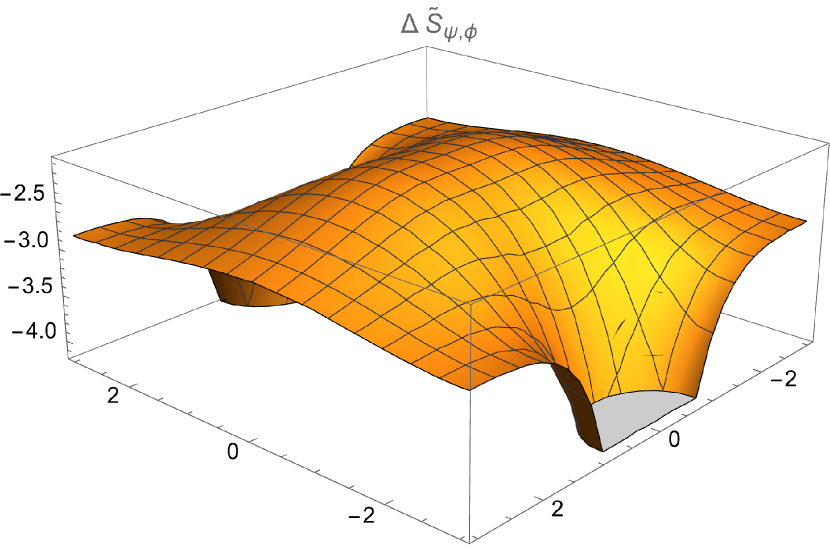
Figure 4: Plot of $\Delta\tilde{S}_{\psi,\phi}$ as a function of the parameter $\gamma$, where both the real and imaginary parts of $\gamma$ range from $-3$ to $3$.

In Fig.4 and Fig.4 we show the numerical results of the function $\Delta S_{\psi,\phi}$ and $\Delta\tilde{S}_{\psi,\phi}$. We can see that the function $\Delta\tilde{S}_{\psi,\phi}$ is negative, which supports the upper bound (5.2.1). While $\Delta S_{\psi,\phi}$ is positive in the same region of $\gamma$.

In the above example, we omitted the term of residue summation as we relied on the findings from section.4.1, where we expanded the function as a series of $\gamma$. However, for large $|\gamma|$, this expansion may pose problems. In the exact expression, the EE $S(\rho(\zeta))$ would include a logarithmic term, potentially encountering the branch cut of the logarithmic function. In the subsequent section, we will briefly discuss the branch cut problem. Nonetheless, it appears that the upper bound (5.2.1) remains correct even for large $|\gamma|$. The upper bound (5.2.1) is indeed a very loose bound. In the case of the perturbed state example, we observe that the upper bound significantly exceeds $|S(\mathcal{T}_{A})|$. Similarly, in the qubit example, this bound appears to be excessively large. It might be plausible to adjust the construction by selecting a different state $|\xi^{\prime}(\theta)\rangle$ (88).

6 Discussion and conclusion

In this paper, we explore a novel operator sum rule (8) applicable to the reduced transition matrix $\mathcal{T}_{A}^{\psi|\phi}$ and the reduced density matrix $\rho_{A}(\theta)$ governing the superposition state $|\xi(\theta)\rangle$. This rule enables the establishment of a relationship between off-diagonal elements and the diagonal elements (10). Moreover, we establish a connection between the pseudo-Rényi entropy and the Rényi entropy. In our previous work [37], we developed a sum rule using discrete Fourier transformation. However, this approach failed to provide a smooth limit for the PE derived from the sum rule for pseudo-Rényi entropy. Through the utilization of our new form of the sum rule, we successfully derive a sum rule for PE (37).

Furthermore, we demonstrate that the transition matrix and the density matrix can be treated uniformly through the analytical continuation of the superposition parameter $\theta$ to a complex variable $\zeta$, as detailed in section.2.2. This approach allows for the extraction of the transition matrix $\mathcal{T}^{\psi|\phi}$ via contour integration at infinity on the $\zeta$ plane. By deforming the contour appropriately, we can readily construct the operator sum rule (8). This analytical continuation becomes indispensable for deriving the complete form of the sum rule for PE. As elucidated in section. 3.4, the accurate sum rule for PE necessitates the inclusion of the residue summation term (46). This assertion is validated through examples discussed in subsequent sections.

In section.5, we delve into the practical implications of the sum rule. One noteworthy application involves gaining insights into the gravity dual of non-Hermitian transition matrices. Our findings reveal that the scaling behavior of connected correlation functions of single trace operators maintains consistency in both the superposition state $|\xi(\theta)\rangle$ and the transition matrix in the large $N$ limit. This observation suggests that a gravity geometry dual should exist for the transition matrix when the superposition state $|\xi(\theta)\rangle$ possesses one. Moreover, the sum rule establishes a connection between two bulk geometries and their on-shell actions. However, as present we lack explicit examples to illustrate this concept. The primary challenge lies in the scarcity of examples demonstrating the exact duality between bulk geometry and boundary states. Recent studies have introduced a class of geometric states known as fixed area states, which are anticipated to exhibit flat entanglement spectra [62][63], see also [64]-[69]. Additionally, there have been some proposals regarding exact states that are dual to fixed area states in boundary CFTs. These investigations hold promise for providing examples that show the significance of the sum rule within the bulk context.

Another intriguing application lies in determining the upper bound of the absolute value of $S(\mathcal{T}_{A}^{\psi|\phi})$. Utilizing the sum rule for PE, this upper bound becomes associated with the upper limit of a superposition state, a topic previously explored in [61]. In our paper, we provide a preliminary bound, which we validate through simple examples. However, we anticipate that the bound could be refined by employing a similar method with a more careful construction of the superposition state $|\xi^{\prime}(\theta)\rangle$. In the work [18], the author proposes that the function (85) is non-positive in QFTs. The sum rule for PE may serve as a valuable tool in either verifying or disproving this proposition.

However, it’s crucial to acknowledge that there are still subtleties regarding the sum rule for PE. Constructing the sum rule for PE hinges on investigating the singularities of the function $\mathcal{N}_{\zeta}S(\rho_{A}(\zeta))$. The entropy function $S(\rho_{A}(\zeta))$ typically involves the logarithmic function. In this paper, we haven’t considered the branch cut arising from the logarithmic function. In all the examples discussed, we assume that one can expand the results with respect to some small parameter, effectively choosing a branch of the logarithmic function. However, if one were to employ the full form of the function $S(\rho_{A}(\zeta))$, it would seem necessary to consider potential modifications due to the branch cut. Currently, we have not found a definitive solution to this issue, but it is an problem we plan to explore in the near future. Nevertheless, it’s important to emphasize that our result regarding the sum rule for PE is applicable in a wide range of examples.

Acknowledgements We would like to thank Xin Gao, Song He, Houwen Wu, Peng Wang, Haitang Yang, Jiaju Zhang, Long Zhao, Yu-Xuan Zhang and Zi-Xuan Zhang for useful discussions. Specially, we would like to thank Jiaju Zhang for early collaboration on this work. WZG is supposed by the National Natural Science Foundation of China under Grant No.12005070 and the Fundamental Research Funds for the Central Universities under Grants NO.2020kfyXJJS041.

Appendix A Second order perturbation of entropy

Given the operator $M$ with $trM=1$, the entropy can be written as

$$S(M)=-\textrm{tr}M\log M=\int_{0}^{\infty}d\beta\left(trM\frac{1}{\beta+M}-\frac{1}{\beta+1}\right).$$ (96)

For the perturbed operator $M+\delta M$ we have

$$S(M+\delta M)=\int_{0}^{\infty}d\beta\left(tr(M+\delta M)\frac{1}{\beta+M+\delta M}-\frac{1}{\beta+1}\right).$$ (97)

We should use the following equation

$$(\beta+M+\delta M)^{-1}$$

$$=[(\beta+M)(1+(\beta+M)^{-1}\delta M)]^{-1}$$

$$=(1+(\beta+M)^{-1}\delta M)^{-1}(\beta+M)^{-1}$$

$$=\left(1-(\beta+M)^{-1}\delta M+(\beta+M)^{-1}\delta M(\beta+M)^{-1}\delta M\right)(\beta+M)^{-1}+O(\delta M^{3}).$$

Now we can find the second order contributions in $S(M+\delta M)$, which is

$$\delta S^{(2)}=\int_{0}^{\infty}d\beta\left(-tr\delta M(\beta+M)^{-1}\delta M(\beta+M)^{-1}\right)$$

$$\phantom{\delta S^{(2)}}+\int_{0}^{\infty}d\beta tr\left(M(\beta+M)^{-1}\delta M(\beta+M)^{-1}\delta M(\beta+M)^{-1}\right)$$

$$\phantom{\delta S^{(2)}}=-\int_{0}^{\infty}d\beta\beta tr\left((\beta+M)^{-2}\delta M(\beta+M)^{-1}\delta M\right).$$ (98)

Appendix B Derivation of the relation (10)

One could derive the relation (10) by utilizing the property of Fourier transformation. By definition, we have

$$\frac{1}{2\pi}\int_{-\pi}^{\pi}d\theta e^{-in\theta}\mathcal{N}_{\theta}^{n}\prod_{j=1}^{m}\langle\xi(\theta)|\mathcal{A}_{j}|\xi(\theta)\rangle$$

$$=\frac{1}{2\pi\langle\phi|\psi\rangle^{n}}\int_{-\pi}^{\pi}d\theta e^{-in\theta}G(e^{i\theta}),$$ (99)

with

$$G(e^{i\theta})=(2+e^{i\theta}\langle\phi|\psi\rangle+e^{-i\theta}\langle\psi|\phi\rangle)^{n-m}\prod_{j=1}^{m}(\langle\phi|+e^{-i\theta}\langle\psi|)\mathcal{A}_{j}(|\phi\rangle+e^{i\theta}|\psi\rangle).$$ (100)

The function $G(e^{i\theta})$ can be expanded as polynomials of $e^{i\theta}$ as long as $n,m$ are integers and $n\geq m$. The highest power is of $e^{in\theta}$ with the coefficient

$$\langle\phi|\psi\rangle^{n-m}\prod_{j=1}^{m}\langle\phi|\mathcal{A}_{j}|\psi\rangle.$$ (101)

This is the only surviving term through Fourier transformation in (100). It can be demonstrated that the result of (100) is

$$\prod_{j=1}^{m}\frac{\langle\phi|\mathcal{A}_{j}|\psi\rangle}{\langle\phi|\psi\rangle}.$$ (102)

Thus, the relation (10) is proven. In section.4.5, where we develop the sum rule for PE with short interval expansion, we arrive at a formula (79) akin to (10). If one begins with the sum rule for pseudo-Rényi entropy (9) and employs the short interval expansion, the same formula (10) can be derived.

References

- [1] L. Amico, R. Fazio, A. Osterloh and V. Vedral, Entanglement in many-body systems, Rev. Mod. Phys. 80, 517 (2008), [arXiv:quant-ph/0703044].
- [2] J. Eisert, M. Cramer and M. B. Plenio, Area laws for the entanglement entropy - a review, Rev. Mod. Phys. 82, 277–306 (2010), [arXiv:0808.3773].
- [3] P. Calabrese and J. Cardy, Entanglement entropy and conformal field theory, J. Phys. A: Math. Gen. 42, 504005 (2009), [arXiv:0905.4013].
- [4] M. Rangamani and T. Takayanagi, Holographic Entanglement Entropy, Lect. Notes Phys. 931, 1–246 (2017), [arXiv:1609.01287].
- [5] S. Ryu and T. Takayanagi, Holographic Derivation of Entanglement Entropy from the anti-de Sitter Space/Conformal Field Theory Correspondence, Phys. Rev. Lett. 96, 181602 (2006), [arXiv:hep-th/0603001].
- [6] V. E. Hubeny, M. Rangamani and T. Takayanagi, A Covariant holographic entanglement entropy proposal, JHEP 07 (2007) 062, [arXiv:0705.0016].
- [7] M. Van Raamsdonk, Building up spacetime with quantum entanglement, Gen. Rel. Grav. 42, 2323 (2010), [arXiv:1005.3035]. [Int. J. Mod. Phys. D19 (2010) 2429].
- [8] A. C. Wall, Maximin Surfaces, and the Strong Subadditivity of the Covariant Holographic Entanglement Entropy, Class. Quant. Grav. 31, no. 22, 225007 (2014), [arXiv:1211.3494[hep-th]].
- [9] A. Almheiri, X. Dong and D. Harlow, Bulk Locality and Quantum Error Correction in AdS/CFT, JHEP 04 (2015) 163, [arXiv:1411.7041].
- [10] X. Dong, D. Harlow and A. C. Wall, Reconstruction of Bulk Operators within the Entanglement Wedge in Gauge-Gravity Duality, Phys. Rev. Lett. 117, no. 2, 021601 (2016), [arXiv:1601.05416[hep-th]].
- [11] G. Penington, Entanglement Wedge Reconstruction and the Information Paradox, JHEP 09 (2020) 002, [arXiv:1905.08255].
- [12] A. Almheiri, N. Engelhardt, D. Marolf and H. Maxfield, The entropy of bulk quantum fields and the entanglement wedge of an evaporating black hole, JHEP 12 (2019) 063, [arXiv:1905.08762].
- [13] A. Strominger, The dS / CFT correspondence, JHEP 10 (2001), 034, [arXiv:0106113[hep-th]].
- [14] J. M. Maldacena, Non-Gaussian features of primordial fluctuations in single field inflationary models, JHEP 05 (2003), 013, [astro-ph/0210603 [astro-ph]].
- [15] K. Doi, J. Harper, A. Mollabashi, T. Takayanagi and Y. Taki, Pseudoentropy in dS/CFT and Timelike Entanglement Entropy, Phys. Rev. Lett. 130, 031601 (2023), [arXiv:2210.09457].
- [16] Y. Nakata, T. Takayanagi, Y. Taki, K. Tamaoka and Z. Wei, New holographic generalization of entanglement entropy, Phys. Rev. D 103, 026005 (2021), [arXiv:2005.13801].
- [17] S. Murciano, P. Calabrese and R. M. Konik, Generalized entanglement entropies in two-dimensional conformal field theory, JHEP 05 (2022) 152, [arXiv:2112.09000].
- [18] A. Mollabashi, N. Shiba, T. Takayanagi, K. Tamaoka and Z. Wei, Pseudo Entropy in Free Quantum Field Theories, Phys. Rev. Lett. 126, 081601 (2021), [arXiv:2011.09648].
- [19] W.-z. Guo, S. He and Y.-X. Zhang, Constructible reality condition of pseudoentropy via pseudo-Hermiticity, JHEP 05 (2023) 021, [arXiv:2209.07308].
- [20] A. Mollabashi, N. Shiba, T. Takayanagi, K. Tamaoka and Z. Wei, Aspects of pseudoentropy in field theories, Phys. Rev. Res. 3, 033254 (2021), [arXiv:2106.03118].
- [21] T. Nishioka, T. Takayanagi and Y. Taki, Topological pseudoentropy, JHEP 09 (2021) 015, [arXiv:2107.01797].
- [22] K. Goto, M. Nozaki and K. Tamaoka, Subregion spectrum form factor via pseudoentropy, Phys. Rev. D 104, L121902 (2021), [arXiv:2109.00372].
- [23] I. Akal, T. Kawamoto, S.-M. Ruan, T. Takayanagi and Z. Wei, Page curve under final state projection, Phys. Rev. D 105, 126026 (2022), [arXiv:2112.08433].
- [24] M. Miyaji, Island for gravitationally prepared state and pseudo entanglement wedge, JHEP 12, 013 (2021), [arXiv:2109.03830].
- [25] W.-z. Guo, S. He and Y.-X. Zhang, On the real-time evolution of pseudo-entropy in 2d CFTs, JHEP 09 (2022) 094, [arXiv:2206.11818].
- [26] Y. Ishiyama, R. Kojima, S. Matsui and K. Tamaoka, Notes on pseudoentropy amplification, PTEP 2022, no.9, 093B10 (2022), [arXiv:2206.14551]
- [27] J. Mukherjee, Pseudo Entropy in U(1) gauge theory, JHEP 10(2022)016, [arXiv:2205.08179].
- [28] Z. Li, Z.-Q. Xiao and R.-Q. Yang, On holographic time-like entanglement entropy, JHEP 04 (2023) 004, [arXiv:2211.14883].
- [29] S. He, J. Yang, Y.-X. Zhang and Z.-X. Zhao, Pseudo-entropy for descendant operators in two-dimensional conformal field theories, arXiv:2301.04891.
- [30] K. Narayan, de Sitter space, extremal surfaces, and time entanglement, Phys. Rev. D 107, 126004 (2023), [arXiv:2210.12963].
- [31] K. Doi, J. Harper, A. Mollabashi, T. Takayanagi and Y. Taki, Timelike entanglement entropy, JHEP 05 (2023) 052, [arXiv:2302.11695].
- [32] T. Kawamoto, S. M. Ruan, Y. k. Suzuki and T. Takayanagi, A half de Sitter holography, JHEP 10 (2023) 137, [arXiv:2306.07575].
- [33] K. Narayan and H. K. Saini, Notes on time entanglement and pseudo-entropy, arXiv:2303.01307.
- [34] S. He, J. Yang, Y. X. Zhang and Z. X. Zhao, Pseudo entropy of primary operators in /-deformed CFTs, arXiv:2305.10984
- [35] X. Jiang, P. Wang, H. Wu and H. Yang, Timelike entanglement entropy and deformation, arXiv:2302.13872.
- [36] A. J. Parzygnat, T. Takayanagi, Y. Taki and Z. Wei, SVD entanglement entropy, JHEP 12 (2023), 123, [arXiv:2307.06531].
- [37] W. z. Guo and J. Zhang, Sum rule for pseudo-Rényi entropy, Phys. Rev. D 109, 106008(2024), arXiv:2308.05261.
- [38] S. He, Y. X. Zhang, L. Zhao and Z. X. Zhao, Entanglement and Pseudo Entanglement Dynamics versus Fusion in CFT, arXiv:2312.02679.
- [39] A. Das, S. Sachdeva and D. Sarkar, Bulk reconstruction using timelike entanglement in (A)dS, arXiv:2312.16056 .
- [40] C. S. Chu and H. Parihar, Time-like entanglement entropy in AdS/BCFT, JHEP 06 (2023) 173, [arXiv:2304.10907].
- [41] X. Jiang, P. Wang, H. Wu and H. Yang, Timelike entanglement entropy in dS3/CFT2, JHEP 08 (2023) 216, [arXiv:2304.10376].
- [42] Z. Chen, Complex-valued Holographic Pseudo Entropy via Real-time AdS/CFT Correspondence, arXiv:2302.14303.
- [43] P. Z. He and H. Q. Zhang, Timelike Entanglement Entropy from Rindler Method, arXiv:2307.09803.
- [44] F. Omidi, Pseudo Rényi Entanglement Entropies For an Excited State and Its Time Evolution in a 2D CFT, arXiv:2309.04112.
- [45] K. Narayan, Further remarks on de Sitter space, extremal surfaces and time entanglement, arXiv:2310.00320.
- [46] W. z. Guo, Y. z. Jiang and Y. Jiang, Pseudo entropy and pseudo-Hermiticity in quantum field theories, JHEP 05 (2024), 071, arXiv:2311.01045.
- [47] H. Kanda, T. Kawamoto, Y. k. Suzuki, T. Takayanagi, K. Tasuki and Z. Wei, Entanglement Phase Transition in Holographic Pseudo Entropy, arXiv:2311.13201.
- [48] K. Shinmyo, T. Takayanagi and K. Tasuki, Pseudo entropy under joining local quenches, arXiv:2310.12542.
- [49] W. z. Guo, S. He and Y. X. Zhang, Relation between timelike and spacelike entanglement entropy, [arXiv:2402.00268 ].
- [50] S. He, P. H. C. Lau and L. Zhao, Detecting quantum chaos via pseudo-entropy and negativity, [arXiv:2403.05875 ].
- [51] N. Lashkari, Relative Entropies in Conformal Field Theory, Phys. Rev. Lett. 113 (2014), 051602, [arXiv:1404.3216].
- [52] E. D’Hoker, X. Dong and C. H. Wu, An alternative method for extracting the von Neumann entropy from Rényi entropies, JHEP 01 (2021), 042, [arXiv:2008.10076].
- [53] J. L. Cardy, O. A. Castro-Alvaredo and B. Doyon, Form factors of branch-point twist fields in quantum integrable models and entanglement entropy, J. Stat. Phys. 130, 129 (2008), [arXiv:0706.3384].
- [54] M. Headrick, Entanglement Rényi entropies in holographic theories, Phys. Rev. D 82, 126010 (2010), [arXiv:1006.0047].
- [55] P. Calabrese, J. Cardy and E. Tonni, Entanglement entropy of two disjoint intervals in conformal field theory II, J. Stat. Mech. (2011) P01021, [arXiv:1011.5482].
- [56] M. A. Rajabpour and F. Gliozzi, Entanglement Entropy of Two Disjoint Intervals from Fusion Algebra of Twist Fields, J. Stat. Mech. (2012) P02016, [arXiv:1112.1225].
- [57] B. Chen and J.-j. Zhang, On short interval expansion of Rényi entropy, JHEP 11 (2013) 164, [arXiv:1309.5453].
- [58] O. Aharony, S. S. Gubser, J. M. Maldacena, H. Ooguri and Y. Oz, Large N field theories, string theory and gravity, Phys. Rept. 323 (2000), 183-386, [[arXiv:hep-th/9905111 ]].
- [59] D. Harlow, TASI Lectures on the Emergence of Bulk Physics in AdS/CFT, PoS TASI2017, 002 (2018), [arXiv:1802.01040].
- [60] X. Dong, The gravity dual of Rényi entropy, Nature Commun. 7, 12472 (2016), [arXiv:1601.06788].
- [61] N. Linden, S. Popescu, and J. A. Smolin, Entanglement of Superpositions, Phys. Rev. Lett. 97, 100502 (2006).
- [62] X. Dong, D. Harlow and D. Marolf, Flat entanglement spectra in fixed-area states of quantum gravity, JHEP 10, 240 (2019), [arXiv:1811.05382 [hep-th]].
- [63] C. Akers and P. Rath, Holographic Renyi Entropy from Quantum Error Correction, JHEP 05, 052 (2019), [arXiv:1811.05171 [hep-th]].
- [64] X. Dong and D. Marolf, One-loop universality of holographic codes, JHEP 03, 191 (2020), [arXiv:1910.06329 [hep-th]].
- [65] X. Dong and H. Wang, Enhanced corrections near holographic entanglement transitions: a chaotic case study, JHEP 11, 007 (2020), [arXiv:2006.10051 [hep-th]].
- [66] D. Marolf, S. Wang and Z. Wang, Probing phase transitions of holographic entanglement entropy with fixed area states, JHEP 12, 084 (2020), [arXiv:2006.10089 [hep-th]].
- [67] C. Akers and G. Penington, Leading order corrections to the quantum extremal surface prescription, JHEP 04, 062 (2021), [arXiv:2008.03319 [hep-th]].
- [68] X. Dong, X. L. Qi and M. Walter, Holographic entanglement negativity and replica symmetry breaking, JHEP 06, 024 (2021), [arXiv:2101.11029 [hep-th]].
- [69] W. z. Guo, Area operator and fixed area states in conformal field theories, Phys. Rev. D 106 (2022) no.6, L061903, [arXiv:2108.03346 [hep-th]].