Are all models wrong? Falsifying binary formation models in gravitational-wave astronomy

Abstract

As the catalogue of gravitational-wave transients grows, several entries appear “exceptional” within the population. Tipping the scales with a total mass of $\approx 150M_{\odot}$, GW190521 likely contained black holes in the pair-instability mass gap. The event GW190814, meanwhile, is unusual for its extreme mass ratio and the mass of its secondary component. A growing model-building industry has emerged to provide explanations for such exceptional events, and Bayesian model selection is frequently used to determine the most informative model. However, Bayesian methods can only take us so far. They provide no answer to the question: does our model provide an adequate explanation for the data? If none of the models we are testing provide an adequate explanation, then it is not enough to simply rank our existing models—we need new ones. In this paper, we introduce a method to answer this question with a frequentist $p$-value. We apply the method to different models that have been suggested to explain GW190521: hierarchical mergers in active galactic nuclei and globular clusters. We show that some (but not all) of these models provide adequate explanations for exceptionally massive events like GW190521.

1 Introduction

The LIGO (Aasi et al., 2015), Virgo (Acernese et al., 2015) and KAGRA (Akutsu et al., 2019) gravitational-wave collaborations have published $\sim 100$ confident compact-binary mergers so far (Abbott et al. (2023)). Several of these events exhibit unusual properties. One such exceptional event is GW190521 (Abbott et al., 2020a), with component masses $m_{1}=85^{+21}_{-14}\text{ }M_{\odot}$ and $m_{2}=66^{+17}_{-18}\text{ }M_{\odot}$ ($90\%$ credible intervals). The formation of these high-mass black holes is difficult to explain in field-binary models due to pair-instability processes (e.g., Heger & Woosley, 2002; Woosley et al., 2007; Belczynski et al., 2016; Woosley, 2017, 2019; Woosley & Heger, 2021), which is expected to produce a black-hole mass gap of approximately $50-135\text{ }M_{\odot}$. However, the precise bounds of this gap are unknown, due especially to uncertainties in nuclear-reaction rates (e.g., Farmer et al., 2019; Costa et al., 2021) as well as envelope retention and mass fallback upon core collapse (e.g., Winch et al., 2024).

Several competing formation channels have been proposed to produce extreme-mass events like GW190521: hierarchical mergers in dense star clusters (e.g., Fragione et al., 2020; Romero-Shaw et al., 2020; Mapelli et al., 2021; Dall’Amico et al., 2021; Arca-Sedda et al., 2021; Liu & Lai, 2021; Kimball et al., 2021) or in accretion disks around active galactic nuclei (AGN) (e.g., Tagawa et al., 2021; Palmese et al., 2021; Samsing et al., 2022; Vajpeyi et al., 2022; Morton et al., 2023), the binary evolution of Population III stars (e.g., Liu & Bromm, 2020; Safarzadeh & Haiman, 2020; Kinugawa et al., 2021; Tanikawa et al., 2021) or mergers of primordial black holes (e.g., De Luca et al., 2021; Clesse & García-Bellido, 2022; Chen et al., 2022).

There are different ways to determine whether a model is consistent with a catalogue of gravitational-wave events, each one corresponding to a different question. These questions can be subtly different, emphasising different ways in which a model can fail to account for the data. Thus, we advocate a multi-pronged approach, which considers a variety of complementary questions. For example, Mould et al. (2023) calculate Bayes factors between different population models for the same event, and thus obtain a relative measure of a models suitability. Meanwhile, Essick et al. (2022) propose an extension to leave-one-out outlier tests, which emphasises the self-consistency of parameterised models analysing different subsets of data. Finally, Payne & Thrane (2023) introduce the concept of the “maximum population likelihood” as a tool for testing a model’s overall goodness of fit for a gravitational-wave catalogue.

In this paper, we build on the foundation laid by the above studies, but explore a different aspect of model testing. We assess whether a particular model can plausibly explain the most exceptional events observed, without directly comparing it to other models. We do this by considering many simulated population catalogues, drawn from the model of interest. We take extremal events from these catalogues and calculate a Bayesian evidence. By computing the Bayesian evidence for many extremal events from different catalogue realizations, we construct a distribution to which we may compare. We use this distribution to calculate a statistic in the form of a $p$-value, which describes how consistent the observed exceptional event is with extremal simulated events.

In Section 2, we develop the statistical framework used in our analysis. In Section 3, we demonstrate a use of our method by assessing the capability of several AGN models and one globular cluster model with hierarchical mergers to produce an event as extreme in total mass as GW190521. We find that it is feasible for both AGN models with sufficiently high natal black hole masses and globular cluster models with zero natal black hole spins to produce GW190521-like events. This suggests that population models that allow for hierarchical mergers can explain the most-massive gravitational-wave events we have observed thus far, and are capable of bridging the proposed pair-instability mass gap (see also, e.g., Fragione et al., 2020; Kimball et al., 2021; Anagnostou et al., 2022).

2 Method

Our starting point is some population model of interest $M$ that defines the prior distribution for parameter(s) $\theta$,

$$\pi(\theta|M),$$ (1)

for example, the distribution for total mass of binary black hole systems. This distribution, in turn, implies a distribution of detected events, which may have a different shape due to selection effects,

$$\pi(\theta|M,\text{det})\propto\pi(\theta|M)\,p_{\text{det}}(\theta).$$ (2)

Here, $p_{\text{det}}(\theta)$ is the probability that an event with parameters $\theta$ is detected.

Since we are interested in extremal events, we next consider a catalogue consisting of $N$ events. Each catalogue has an apparently most extreme event such that the maximum likelihood estimator for that event $\widehat{\theta}$ is larger (or smaller) than all other events,

$$\widehat{\theta}_{i}\lessgtr\widehat{\theta}_{j\neq i}.$$ (3)

There is some distribution of $\theta$ for these apparently most extreme events,

$$\pi(\theta_{\text{ext}}|M,\text{det},N).$$ (4)

For example, this distribution could represent the distribution of total mass for the apparently most massive event in a catalogue of $N=100$ events.

In the limit where $\theta_{\text{ext}}$ is measured precisely, then the maximum likelihood estimator approaches the true parameter value

$$\widehat{\theta}_{\text{ext}}\rightarrow\theta_{\text{ext}},$$ (5)

and so the apparently most extreme event is the most extreme event. In this limit, one may calculate a $p$-value for an extremal event with $\widehat{\theta}_{\text{ext}}$ in a catalogue with $N$ events,

$$p\equiv \int_{\Gamma_{1}}d\theta\,\pi(\theta_{\text{ext}}|M,\text{det},N)$$ (8)

$$\Gamma_{1}= \bigg{\{}\pi(\theta_{\text{ext}}|M,\text{det},N)<\pi(\widehat{\theta}_{\text{ext}}|M,\text{det},N)\bigg{\}}.$$ (9)

This $p$-value corresponds to the fraction of draws from $\pi(\theta_{\text{ext}}|M,\text{det},N)$ that produce a prior probability density smaller than what we obtain for the observed value of $\widehat{\theta}_{\text{ext}}$. If the observed value of total mass is unusual—either too small or too big—then $\pi(\widehat{\theta}_{\text{ext}}|M,\text{det},N)$ will be small, and so the resulting $p$-value will be accordingly small. On the other hand, if the observed total mass is typical given the model, then $\pi(\widehat{\theta}_{\text{ext}}|M,\text{det},N)$ is large, and so $p$ is ${\cal O}(1)$.

In reality, we do not measure $\theta_{\text{ext}}$ precisely. Rather, each measurement is characterised with a precision determined by the likelihood function ${\cal L}(d|\theta_{\text{ext}})$. In order to include measurement uncertainty, we define a new metric, “the normalised evidence”:

$$\overline{\mathcal{Z}}\equiv \overline{\pi(\theta_{\text{ext}}|M,\text{det},N)}$$

$$= \frac{\int d\theta\,{\cal L}(d|\theta_{\text{ext}})\pi(\theta_{\text{ext}}|M,\text{det},N)}{\int d\theta\,{\cal L}(d|\theta_{\text{ext}})\pi(\theta_{\text{ext}}|U)},$$ (10)

where the overline denotes an average over measurement uncertainty, and $\pi(\theta|U)$ is a prior uniform in the parameter of interest. In the high signal-to-noise ratio (SNR) limit, the likelihood function becomes a delta function peaked at the true parameter values $\theta_{\text{true}}$, so

$$\overline{\mathcal{Z}}\rightarrow \frac{\int d\theta\,\delta(\theta_{\text{ext}}-\theta_{\text{true}})\pi(\theta_{\text{ext}}|M,\text{det},N)}{\int d\theta\,\delta(\theta_{\text{ext}}-\theta_{\text{true}})\pi(\theta_{\text{ext}}|U)},$$ (11)

which simplifies to

$$\overline{\mathcal{Z}}\rightarrow \frac{\pi(\theta_{\text{true}}|M,\text{det},N)}{\pi(\theta_{\text{true}}|U)}.$$ (12)

In the high SNR limit, $\overline{\mathcal{Z}}$ approaches the ratio of prior probability densities at $\theta_{\text{true}}$. Thus, the denominator of Eq. 2 ensures $\overline{\mathcal{Z}}$ tracks the parameter of interest. By constructing an empirical distribution of $\overline{\mathcal{Z}}$ with simulated data—denoted $\pi(\overline{\mathcal{Z}}|M,\text{det},N)$—we can again calculate a $p$-value quantifying if the observed value ${\overline{\mathcal{Z}}}$ is unusual compared to the distribution expected from simulation:

$$p\equiv \int_{\Gamma_{2}}d\overline{\mathcal{Z}}^{\prime}\,\pi(\overline{\mathcal{Z}}^{\prime}|M,\text{det},N)$$ (13)

$$\Gamma_{2}= \bigg{\{}\pi(\overline{\mathcal{Z}}^{\prime}|M,\text{det},N)<\pi(\overline{\mathcal{Z}}|M,\text{det},N)\bigg{\}}.$$ (14)

If the observed value of total mass is unusual—after taking into account measurement uncertainty—then ${\overline{\mathcal{Z}}}$ will be small, and so the resulting $p$-value will be accordingly small, whereas if ${\overline{\mathcal{Z}}}$ is large, $p$ is ${\cal O}(1)$. Moreover, this procedure reproduces Eq. 8 in the high signal-to-noise ratio limit.

3 Demonstration

To demonstrate the above formalism, we test the ability of different models to explain the total mass $m_{\text{tot}}$ of the event GW190521. We consider four models:

• Gayathri et al. (2023) propose a model for binary black hole formation in an AGN disk with hierarchical mergers. We consider three variations of this model, each with a different maximum natal black hole mass $m_{\text{max}}=15M_{\odot},50M_{\odot}\text{ and }75\text{M}_{\odot}$. These three models are labeled “AGN.”

• Rodriguez et al. (2019)’s model for binary black hole assembly in globular clusters. In particular, we consider the model variation with natal black hole spin $\chi_{\text{birth}}=0$. This model is labeled “Globular Cluster”.

For each model, we simulate $N=100$ events for the LIGO H1 and L1 observatories operating at design sensitivity. We create $n=100$ catalogues of simulated events ($10^{4}$ events in total). Each event is injected into Gaussian noise colored by the amplitude spectral density noise curves of design-sensitivity LIGO. Each detection has network SNR $>12$. For each catalogue, we find the event with highest total mass. Strictly speaking, this is not equivalent to selecting the event with the largest apparent $m_{\text{tot}}$. By only choosing the truly most massive event, rather than the apparently most massive event, the Eq. 4 distribution is slightly skewed to higher total masses. This leads to a smaller, more conservative $p$-value with a more manageable computational cost. The distributions of maximum total mass for each model are shown in Fig. 1.

Figure 1: The distribution of total mass $m_{\text{tot}}$ for different models. The solid curves are the original models while the histograms show the distribution of the most massive event in each simulated catalogue. We consider three variations of the AGN model from Gayathri et al. (2023) with different maximum black hole masses $m_{\text{max}}$ (blue, orange, green). We include a globular cluster model from Rodriguez et al. (2019) (pink).

For the most massive event in each catalogue, we calculate ${\overline{\cal Z}}$ (Eq. 2) with the nested sampler dynesty (Speagle, 2020) as implemented in Bilby (Ashton et al., 2019). Our initial run uses the IMRPhenomPv2 waveform approximant (Schmidt et al., 2012). We choose boundary values of the component mass priors to include the range of masses in the injection set. We choose dimensionless spin magnitude priors to be truncated Gaussians about 0.7, reflecting their dynamical evolution history (see, e.g., Stevenson et al., 2017). We then use importance sampling to reweight the result to obtain the marginal likelihood that we would have obtained using $\pi(\theta_{\text{ext}}|M,\text{det},N)$; see, e.g., Thrane & Talbot (2019). We estimate $\pi(\theta_{\text{ext}}|M,\text{det},N)$ by fitting each histogram in Fig. 1 with a kernel density estimator.

As an example, in Fig. 2 we plot $\ln\overline{\cal Z}$ versus the maximum-likelihood value of $m_{\text{tot}}$ for the most massive event in each simulated catalogue, for the $m_{\text{max}}=50M_{\odot}$ AGN model. The most common value of $m_{\text{tot}}$ is $\approx 130\,\mathrm{M_{\odot}}$, consistent with expectations from Fig. 1. As expected, these typical values of $m_{\text{tot}}$ tend to produce relatively large values of $\ln\overline{\cal Z}$.

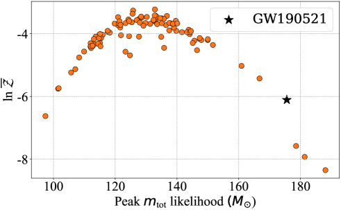
Figure 2: Log-normalised evidence $\ln{\overline{\mathcal{Z}}}$ versus peak total mass likelihood for the most-massive events of the $m_{\text{max}}=50M_{\odot}$ AGN model. Total masses are the median posterior value. Lower $\ln{\overline{\mathcal{Z}}}$ values correspond to catalogues that are relatively unusual—either because the maximum total mass is either unusually small or unusually large. The highest values of $\ln{\overline{\mathcal{Z}}}$ correspond to typical catalogues with usual values for the maximum total mass. The log-normalised evidence for GW190521, calculated using this model, is also plotted against the peak total mass likelihood of GW190521.

Continuing with the $m_{\text{max}}=50M_{\odot}$ AGN model as an example, we use the empirical distribution of $\ln\overline{\cal Z}$ (shown in orange in Fig. 3) to calculate a $p$-value for GW190521 ($\ln\overline{\cal Z}=-6.1$; black-dashed line). Since 96% of the simulations produce $\ln\overline{\cal Z}$ values larger than the one obtained for GW190521, the $p$-value is $p=0.04$ (disfavored at the two-sigma level). This implies the total mass of GW190521 is somewhat unusual (at the two sigma level) compared to the distribution of expected most massive events after $N=100$ events and given the Gayathri et al. (2023) model.

We repeat this process for the $m_{\text{max}}=15M_{\odot}\text{ and }75M_{\odot}$ AGN models, as well as the globular cluster model. We summarise the results in Table 1; see also Fig. 3. We find $p\simeq 0$ for the $m_{\text{max}}=15M_{\odot}$ AGN model, indicating this model almost never produces an event as massive as GW190521. We find the $m_{\text{max}}=75M_{\odot}$ AGN model has $p=0.52$, suggesting the model produces GW190521-like events often. Finally, we find the globular cluster model has $p=0.24$, suggesting that it is reasonable to draw a GW190521-like event from this model.

Table 1: Associated $p$-value for each model based on AGN natal black hole mass $m_{\text{max}}$ or globular cluster (GC) scenario.

Model	$15M_{\odot}$	$50M_{\odot}$	$75M_{\odot}$	GC
$p$-value	$\sim 0$	$0.04$	$0.52$	$0.24$

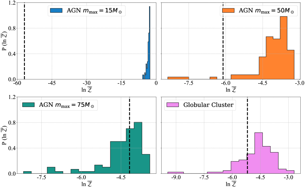
Figure 3: Probability distribution of log-normalised evidence $(\ln{\overline{\mathcal{Z}}})$ for distributions of most-massive, detectable events drawn from Eq. 4 (histograms), against $\ln{{\overline{\mathcal{Z}}}^{\prime}}$, the log-normalised evidence for GW190521 (black-dashed line), for (from left to right, top to bottom) AGN models with $m_{\text{max}}=15\text{}M_{\odot}\text{ (blue), }50\text{}M_{\odot}\text{ (orange) }\text{ and }75\text{}M_{\odot}\text{ (green)}$, as well as a globular cluster model with $\chi_{\text{birth}}=0$ (pink). The $p$-value calculation in Eq. 13 is the integral over the region to the left of $\ln{{\overline{\mathcal{Z}}}^{\prime}}$.

4 Discussion

We have demonstrated the use of our statistical framework, which makes use of the “normalised evidence” $\overline{\mathcal{Z}}$ in testing several models of binary formation using the exceptional event GW190521. We rule out the AGN model with $m_{\text{max}}=15\text{}M_{\odot}$. The AGN model with $m_{\text{max}}=50\text{}M_{\odot}$ is slightly disfavoured in explaining GW190521 (at the two-sigma level). The AGN model with $m_{\text{max}}=75\text{}M_{\odot}$ and the globular cluster model plausibly provide adequate explanations for GW190521.

For future work we propose to apply this method more broadly in order to falsify models as explanations for exceptional events. Key questions include:

• Which models are consistent with the most massive binary black holes?

• Which models are consistent with the most extreme spins?

• Which models are consistent with the most extreme mass ratios, such as GW190814 (Abbott et al., 2020b)?

• Similarly, which models are consistent with the smallest secondary masses, like the $m_{2}=2.6M_{\odot}$ object observed in GW190814 (Abbott et al., 2020b)?

There are many ways to evaluate the explanatory power of different population models, each of which provides the answer to a different question. The Bayes factor can be used to determine which of two population models provides a better description of the data (e.g. Mould et al., 2023). We note it may be useful to determine if none of the models tested provide an adequate fit—something we do not learn from the Bayes factor, which is a relative comparison of models.

Leave-one-out analyses can be used to determine if one event is a statistical outlier with respect to the rest of the population (e.g. Essick et al., 2022). Our method may be similarly extended to examine whether fits to the entire observed population can explain the most exceptional events observed. If the model is fit to the data and still struggles to explain an exceptional event, it is clearly inadequate.

Finally, the “maximum population likelihood” may be used to test a model’s goodness of fit to observed events (Payne & Thrane, 2023). This method characterises a model’s fit to an entire catalogue of events, requiring parameter estimation on all events in many simulated catalogues. Our method focuses only on exceptional events, and thus vastly reduces the total computation required.

Our framework is an example of “model criticism” (Romero-Shaw et al., 2022). It is a posterior predictive check in which one infers a model distribution from observed data, then compares samples from that distribution back to data, to check for consistency (e.g., Fishbach et al., 2020). Specifically, we perform a posterior predictive check on a model for a single observed extreme event. This requires adopting a frequentist approach, as opposed to an entirely Bayesian framework, as well as comparisons of events’ “normalised evidences”, rather than comparisons of their posteriors.

References

- Aasi et al. (2015) Aasi et al., J. 2015, Class. Quantum Grav., 32, 074001, doi: 10.1088/0264-9381/32/7/074001
- Abbott et al. (2020a) Abbott et al., R. 2020a, Phys. Rev. Lett., 125, 101102, doi: 10.1103/PhysRevLett.125.101102
- Abbott et al. (2020b) —. 2020b, ApJL, 896, L44, doi: 10.3847/2041-8213/ab960f
- Abbott et al. (2023) —. 2023, Phys. Rev. X, 13, 041039, doi: 10.1103/PhysRevX.13.041039
- Acernese et al. (2015) Acernese, F., Agathos, M., Agatsuma, K., et al. 2015, Class. Quantum Grav., 32, 024001, doi: 10.1088/0264-9381/32/2/024001
- Akutsu et al. (2019) Akutsu, T., Ando, M., Arai, K., et al. 2019, Nat Astron, 3, 35, doi: 10.1038/s41550-018-0658-y
- Anagnostou et al. (2022) Anagnostou, O., Trenti, M., & Melatos, A. 2022, ApJ, 941, 4, doi: 10.3847/1538-4357/ac9d95
- Arca-Sedda et al. (2021) Arca-Sedda, M., Paolo Rizzuto, F., Naab, T., et al. 2021, ApJ, 920, 128, doi: 10.3847/1538-4357/ac1419
- Ashton et al. (2019) Ashton, G., Hübner, M., Lasky, P. D., et al. 2019, ApJS, 241, 27, doi: 10.3847/1538-4365/ab06fc
- Belczynski et al. (2016) Belczynski, K., Heger, A., Gladysz, W., et al. 2016, A&A, 594, A97, doi: 10.1051/0004-6361/201628980
- Chen et al. (2022) Chen, Z.-C., Yuan, C., & Huang, Q.-G. 2022, Physics Letters B, 829, 137040, doi: 10.1016/j.physletb.2022.137040
- Clesse & García-Bellido (2022) Clesse, S., & García-Bellido, J. 2022, Physics of the Dark Universe, 38, 101111, doi: 10.1016/j.dark.2022.101111
- Costa et al. (2021) Costa, G., Bressan, A., Mapelli, M., et al. 2021, Monthly Notices of the Royal Astronomical Society, 501, 4514, doi: 10.1093/mnras/staa3916
- Dall’Amico et al. (2021) Dall’Amico, M., Mapelli, M., Di Carlo, U. N., et al. 2021, Monthly Notices of the Royal Astronomical Society, 508, 3045, doi: 10.1093/mnras/stab2783
- De Luca et al. (2021) De Luca, V., Desjacques, V., Franciolini, G., Pani, P., & Riotto, A. 2021, Phys. Rev. Lett., 126, 051101, doi: 10.1103/PhysRevLett.126.051101
- Essick et al. (2022) Essick, R., Farah, A., Galaudage, S., et al. 2022, ApJ, 926, 34, doi: 10.3847/1538-4357/ac3978
- Farmer et al. (2019) Farmer, R., Renzo, M., de Mink, S. E., Marchant, P., & Justham, S. 2019, ApJ, 887, 53, doi: 10.3847/1538-4357/ab518b
- Fishbach et al. (2020) Fishbach, M., Essick, R., & Holz, D. E. 2020, ApJL, 899, L8, doi: 10.3847/2041-8213/aba7b6
- Fragione et al. (2020) Fragione, G., Loeb, A., & Rasio, F. A. 2020, ApJL, 902, L26, doi: 10.3847/2041-8213/abbc0a
- Gayathri et al. (2023) Gayathri, V., Wysocki, D., Yang, Y., et al. 2023, ApJL, 945, L29, doi: 10.3847/2041-8213/acbfb8
- Heger & Woosley (2002) Heger, A., & Woosley, S. E. 2002, ApJ, 567, 532, doi: 10.1086/338487
- Kimball et al. (2021) Kimball, C., Talbot, C., Berry, C. P. L., et al. 2021, ApJL, 915, L35, doi: 10.3847/2041-8213/ac0aef
- Kinugawa et al. (2021) Kinugawa, T., Nakamura, T., & Nakano, H. 2021, Monthly Notices of the Royal Astronomical Society: Letters, 501, L49, doi: 10.1093/mnrasl/slaa191
- Liu & Bromm (2020) Liu, B., & Bromm, V. 2020, ApJL, 903, L40, doi: 10.3847/2041-8213/abc552
- Liu & Lai (2021) Liu, B., & Lai, D. 2021, Monthly Notices of the Royal Astronomical Society, 502, 2049, doi: 10.1093/mnras/stab178
- Mapelli et al. (2021) Mapelli, M., Dall’Amico, M., Bouffanais, Y., et al. 2021, Monthly Notices of the Royal Astronomical Society, 505, 339, doi: 10.1093/mnras/stab1334
- Morton et al. (2023) Morton, S. L., Rinaldi, S., Torres-Orjuela, A., et al. 2023, Phys. Rev. D, 108, 123039, doi: 10.1103/PhysRevD.108.123039
- Mould et al. (2023) Mould, M., Gerosa, D., Dall’Amico, M., & Mapelli, M. 2023, Monthly Notices of the Royal Astronomical Society, 525, 3986, doi: 10.1093/mnras/stad2502
- Palmese et al. (2021) Palmese, A., Fishbach, M., Burke, C. J., Annis, J., & Liu, X. 2021, ApJL, 914, L34, doi: 10.3847/2041-8213/ac0883
- Payne & Thrane (2023) Payne, E., & Thrane, E. 2023, Phys. Rev. Res., 5, 023013
- Rodriguez et al. (2019) Rodriguez, C. L., Zevin, M., Amaro-Seoane, P., et al. 2019, Phys. Rev. D, 100, 043027, doi: 10.1103/PhysRevD.100.043027
- Romero-Shaw et al. (2020) Romero-Shaw, I., Lasky, P. D., Thrane, E., & Bustillo, J. C. 2020, ApJL, 903, L5, doi: 10.3847/2041-8213/abbe26
- Romero-Shaw et al. (2022) Romero-Shaw, I. M., Thrane, E., & Lasky, P. D. 2022, Publ. Astron. Soc. Aust., 39, e025, doi: 10.1017/pasa.2022.24
- Safarzadeh & Haiman (2020) Safarzadeh, M., & Haiman, Z. 2020, ApJL, 903, L21, doi: 10.3847/2041-8213/abc253
- Samsing et al. (2022) Samsing, J., Bartos, I., D’Orazio, D. J., et al. 2022, Nature, 603, 237, doi: 10.1038/s41586-021-04333-1
- Schmidt et al. (2012) Schmidt, P., Hannam, M., & Husa, S. 2012, Phys. Rev. D, 86, 104063, doi: 10.1103/PhysRevD.86.104063
- Speagle (2020) Speagle, J. S. 2020, Monthly Notices of the Royal Astronomical Society, 493, 3132, doi: 10.1093/mnras/staa278
- Stevenson et al. (2017) Stevenson, S., Berry, C. P. L., & Mandel, I. 2017, Monthly Notices of the Royal Astronomical Society, 471, 2801, doi: 10.1093/mnras/stx1764
- Tagawa et al. (2021) Tagawa, H., Kocsis, B., Haiman, Z., et al. 2021, ApJ, 908, 194, doi: 10.3847/1538-4357/abd555
- Tanikawa et al. (2021) Tanikawa, A., Kinugawa, T., Yoshida, T., Hijikawa, K., & Umeda, H. 2021, Monthly Notices of the Royal Astronomical Society, 505, 2170, doi: 10.1093/mnras/stab1421
- Thrane & Talbot (2019) Thrane, E., & Talbot, C. 2019, Pub. Astron. Soc. Aust., 36, E010
- Vajpeyi et al. (2022) Vajpeyi, A., Thrane, E., Smith, R., McKernan, B., & Ford, K. E. S. 2022, ApJ, 931, 82, doi: 10.3847/1538-4357/ac6180
- Winch et al. (2024) Winch, E. R. J., Vink, J. S., Higgins, E. R., & Sabhahitf, G. N. 2024, Monthly Notices of the Royal Astronomical Society, 529, 2980, doi: 10.1093/mnras/stae393
- Woosley (2017) Woosley, S. E. 2017, ApJ, 836, 244, doi: 10.3847/1538-4357/836/2/244
- Woosley (2019) —. 2019, ApJ, 878, 49, doi: 10.3847/1538-4357/ab1b41
- Woosley et al. (2007) Woosley, S. E., Blinnikov, S., & Heger, A. 2007, Nature, 450, 390, doi: 10.1038/nature06333
- Woosley & Heger (2021) Woosley, S. E., & Heger, A. 2021, ApJL, 912, L31, doi: 10.3847/2041-8213/abf2c4