Dynamics of a higher-dimension Einstein-Scalar-Gauss-Bonnet cosmology

Abstract

We study the dynamics of the field equations in a five-dimensional spatially flat Friedmann-Lemaître-Robertson-Walker metric in the context of a Gauss-Bonnet-Scalar field theory where the quintessence scalar field is coupled to the Gauss-Bonnet scalar. Contrary to the four-dimensional Gauss-Bonnet theory, where the Gauss-Bonnet term does not contribute to the field equations, in this five-dimensional Einstein-Scalar-Gauss-Bonnet model, the Gauss-Bonnet term contributes to the field equations even when the coupling function is a constant. Additionally, we consider a more general coupling described by a power-law function. For the scalar field potential, we consider the exponential function. For each choice of the coupling function, we define a set of dimensionless variables and write the field equations into a system of ordinary differential equations. We perform a detailed analysis of the dynamics for both systems and classify the stability of the equilibrium points. We determine the presence of scaling and super-collapsing solutions using the cosmological deceleration parameter. This means that our models can explain the Universe’s early and late-time acceleration phases. Consequently, this model can be used to study inflation or as a dark energy candidate.

I Introduction

The Universe has been observed to be undergoing accelerated expansion in recent cosmological history. The simplest explanation for this is the cosmological constant. However, the issue and the possibility of a dynamic nature have led to two main approaches to its description. The first approach maintains general relativity and introduces the concept of dark energy, which can account for all forms of new, exotic sectors that can be sources of acceleration Copeland:2006wr ; Cai:2009zp . The second step is to attribute the new degrees of freedom to modifications of the gravitational interaction CANTATA:2021ktz ; Capozziello:2011et ; Nojiri:2010wj , namely to extended theories with general relativity as a limit but generally have a richer structure. Additionally, there is evidence that most of the Universe’s matter content is in Cold Dark Matter (CDM) Liddle:1993fq ; Planck:2018vyg ; Abdalla:2022yfr . Although most cosmologists believe that dark matter should correspond to some particle beyond the Standard Model, the fact that it has not been directly detected in the accelerators led to the investigation of many models in which dark matter can have, partially or entirely, gravitational origin Nojiri:2006gh ; Famaey:2011kh ; Sebastiani:2016ras ; Addazi:2021xuf . Modified theories of gravity may arise by extending the Einstein-Hilbert action in a suitable way, such as in $F(R)$ DeFelice:2010aj and $F(G)$ Nojiri:2005jg ; DeFelice:2008wz gravity, in Lovelock construction lov1 ; lov2 ; lov3 ; Deruelle:1989fj , in Horndeski gravity Horndeski:1974wa , in generalized galileon theories DeFelice:2010nf ; Deffayet:2011gz , etc. Nevertheless, one can construct gravitational modifications starting from the equivalent torsional formulation of gravity Pereira ; Maluf:2013gaa and build theories such as $F(T)$ gravity Cai:2015emx ; Ferraro:2006jd ; Linder:2010py , $F(T,T_{G})$ gravity Kofinas:2014owa , $F(T,B)$ gravity Bahamonde:2015zma , etc. In this framework, one can also introduce scalar fields, i.e. constructing scalar-torsion theories Geng:2011aj , allowing for non-minimal Geng:2011aj ; Geng:2011ka ; Gonzalez-Espinoza:2020jss ; Paliathanasis:2021nqa ; Gonzalez-Espinoza:2021qnv ; Toporensky:2021poc or derivative Kofinas:2015hla couplings with torsion or more general constructions Geng:2012vtr ; Skugoreva:2014ena ; Jarv:2015odu ; Skugoreva:2016bck ; Hohmann:2018rwf ; Hohmann:2018vle ; Hohmann:2018ijr ; Hohmann:2018dqh ; Emtsova:2019qsl , then can even be the teleparallel version of Horndeski theories Bahamonde:2019shr ; Bahamonde:2020cfv ; Bahamonde:2021dqn ; Bernardo:2021izq , or allow for a non-minimal scalar-torsion coupling and with boundary term and fermion-torsion coupling. Recently, in Kucukakca:2013mya ; Kucukakca:2014vja ; Gecim:2017hmn performed a detailed study of the teleparallel dark energy in the light of Noether point symmetries. In MohseniSadjadi:2015yex ; MohseniSadjadi:2016ukp , the onset of cosmic acceleration from a matter-dominated era ending to a de Sitter phase was studied in the framework of coupled quintessence-torsion model in teleparallel gravity. Late-time acceleration driven by shift-symmetric Galileon in the presence of torsion was investigated in Banerjee:2018yyi . Moreover, scalar fields or modified gravity models can be used at galactic scales for the dark matter explanation Sharma:2019yix ; Sharma:2020vex .

While four-dimensional spacetime accurately describes the universe, studying theories in higher dimensions is beneficial for several reasons. Spacetime becomes more mathematically tractable when using theories with more than four dimensions ($N>4$), making calculations easier. The field equations for apparent vacuum in five dimensions can be shown to yield Einstein’s field equations in 4D with matter because what is commonly referred to as matter can be seen as the result of the embedding in a five-dimensional flat manifold Wesson:2014raa ; Wesson .

Five-dimensional field theory directly extends the four-dimensional spacetime in Einstein’s General Relativity. It is considered the minimum dimension in higher-dimensional theories, including ten-dimensional supersymmetry, eleven-dimensional supergravity, and string theory Wesson . Other theories in five dimensions include Induced-matter theory, a specific case of Kaluza-Klein theory Wesson-Ponce ; Castillo-Felisola:2016kpe , and Membrane theory Randall:1999vf ; Arkani-Hamed:1998sfv , where authors explore a 3-brane in a five-dimensional manifold. Black holes have also been studied in the context of a five-dimensional Einstein-Gauss-Bonnet cosmology Ghosh:2016ddh .

The natural generalization of General Relativity in higher-dimensional spaces is Lovelock’s theory of gravity lov1 ; lov2 ; lov3 ; Deruelle:1989fj . Lovelock’s gravity is a second-order theory that reduces to General Relativity in the case of four-dimensional spacetime.

The Gauss-Bonnet theory is part of Lovelock’s gravity, where the Gauss-Bonnet scalar modifies the Einstein-Hilbert Action. The Gauss-Bonnet scalar is a topological invariant in four dimensions, making the theory equivalent to General Relativity Armaleo:2017lgr . However, the four-dimensional Einstein-scalar-Gauss-Bonnet gravity has been previously introduced Nojiri:2005vv ; Nojiri:2006je ; Cognola:2006sp ; Nojiri:2007te ; Padmanabhan:2013xyr ; Chakraborty:2018scm ; Fomin:2018typ , where the scalar field interacts with the Gauss-Bonnet scalar through a non-constant function. In this theory, the mass of the scalar field depends on the topological invariant of the Gauss-Bonnet scalar Kanti:2015pda ; Hikmawan:2015rze ; Motaharfar:2016dqt ; Rashidi:2020wwg . As a result, there is a non-zero contribution of the Gauss-Bonnet scalar in the gravitational theory.

For it to contribute significantly to the four-dimensional model, in Millano:2023czt ; Millano:2023gkt , the authors considered various coupling functions between the Gauss-Bonnet scalar and the scalar field. It was found that in four dimensions, stationary points describe zero acceleration and de Sitter solutions.

In the present work, we extend the previous studies to a five-dimensional geometry, where the Gauss-Bonnet scalar contributes to the field equations even if the coupling function is set to be constant. This work considers a constant and linear coupling function between the Gauss-Bonnet scalar and a quintessence scalar field with its exponential potential.

Dynamical system methods have been widely used in cosmology to obtain relevant information from systems of ordinary differential equations that describe the early and late-time evolution of the models Leon:2020lnr ; Millano:2023vny ; Leon:2023idl ; Millano:2024rog . In particular, as mentioned before, in references Millano:2023czt ; Millano:2023gkt , the authors studied the asymptotic behaviour and dynamics of four-dimensional Einstein-Gauss-Bonnet cosmologies with and without matter with different coupling between the Gauss-Bonnet invariant and the scalar field.

In cosmology, the deceleration parameter, denoted as $q$, indicates whether a stationary point represents an accelerated solution. When combined with the knowledge that a stationary point could act as a model’s early or late-time attractor, we can determine the potential evolution of the cosmological model from early to late times. A value $q>0$ indicates an eventual collapsing universe, while a value $q<0$ signifies an accelerated universe. Specifically, when $q=-1$, it represents a de Sitter solution. Our five-dimensional model can exhibit both of these behaviours and in addition, it can have stationary points that represent scaling solutions, where $q=-1+\frac{3\lambda^{2}}{4}$.

This study is self-contained and organized as follows: In section II, we briefly review the primary tools used to analyze the dynamical systems that appear throughout this work.

In section III, we present the Action Integral for the five-dimensional Gauss-Bonnet model and derive the corresponding field equations. In section III.1 we select the coupling function $f$ to be constant since, in this model, the Gauss-Bonnet term is not a total derivative, and it alone contributes to the field equations. The dynamical system analysis for the model with constant coupling function is performed in section III.1.1. We also perform numerical integration of the two-dimensional dynamical system and present a possible late-time evolution for the model and the behaviour of the deceleration parameter. Additionally, section III.1.2 presents an alternative dynamical systems formulation for this constant coupling function model with illustrative topological properties. On the other hand, section III.2 considers a more general coupling function; that is, $f$ is a linear function. The dynamical system analysis for this choice of coupling function is performed in section III.2.1. A projection in two dimensions is presented in section III.2.2, where we perform an approximated numerical analysis of the stability of the projected stationary points. At the end of this section, one possible late-time evolution of the model is presented using numerical integration and the deceleration parameter. Finally, in section IV, we present the conclusions of our work.

II Dynamical systems techniques

In this section, we briefly review the standard dynamical system tools that will be used throughout this work. Consider a system of nonlinear ordinary differential equations given by

$$\dot{\mathbf{x}}=f(\mathbf{x}),$$ (1)

where $\mathbf{x}=(x_{1},x_{2},\ldots,x_{n})$ and $\dot{\mathbf{x}}=\frac{d\mathbf{x}}{dt}=\left(\frac{dx_{1}}{dt},\frac{dx_{2}}{dt},\ldots\frac{dx_{n}}{dt}\right)$. We consider $\textbf{f}=(f_{1},f_{2},\ldots,f_{n})$ to be of class $C^{1}(E)$ and $E$ is an open subset of $\mathbb{R}^{n}$. We observe that system (1) is autonomous in the sense that there is no explicit dependence on time as opposed to systems like $\dot{\mathbf{x}}=g(\mathbf{x},t)$. Now we present the following definitions

Definition 1.

An equilibrium point of system (1) is any point $\mathbf{x^{*}}\in\mathbb{R}^{n}$ such that $\mathbf{f}(\mathbf{x^{*}})=0$.

Definition 2.

The linearization matrix of system (1) also called Jacobian matrix is

$$\mathbf{J}=D\mathbf{f}=\begin{bmatrix}\frac{\partial f_{1}}{\partial x_{1}}&\frac{\partial f_{1}}{\partial x_{2}}&\cdots&\frac{\partial f_{1}}{\partial x_{n}}\\ \\ \frac{\partial f_{2}}{\partial x_{1}}&\frac{\partial f_{2}}{\partial x_{2}}&\cdots&\frac{\partial f_{2}}{\partial x_{n}}\\ \vdots&\vdots&\ddots&\vdots\\ \frac{\partial f_{n}}{\partial x_{1}}&\frac{\partial f_{n}}{\partial x_{2}}&\cdots&\frac{\partial f_{n}}{\partial x_{n}}\end{bmatrix}$$ (2)

Definition 3.

An equilibrium point $\mathbf{x^{*}}$ is called hyperbolic if none of the eigenvalues of $\mathbf{J}(\mathbf{x^{*}})$ have zero real part. It is called non-hyperbolic if $\mathbf{J}(\mathbf{x^{*}})$ has eigenvalues with zero real part.

Definition 4.

A hyperbolic equilibrium point $\mathbf{x^{*}}$ of system (1) is called

1. an attractor (stable) if all the eigenvalues of $\mathbf{J}(\mathbf{x^{*}})$ have negative real part,

2. a source (unstable) if all the eigenvalues of $\mathbf{J}(\mathbf{x^{*}})$ have positive real part,

3. a saddle (unstable) if $\mathbf{J}(\mathbf{x^{*}})$ has at least one eigenvalue with a positive real part and at least one with a negative real part.

Definition 5.

A set of non-isolated equilibrium points is normally hyperbolic if the only eigenvalues with zero real part are those whose corresponding eigenvectors are tangent to the set. The sign of the real part of the remaining nonzero eigenvalues determines the stability of the set (or family).

Definitions 1-4 are taken from Perko and definition 5 is from ColeyBook . The following result establishes the main tool that will be used to study the dynamical systems in this work.

Theorem 1 (Hartman-Grobman).

ColeyBook The qualitative structure of the nonlinear system (1) near a hyperbolic equilibrium point $\mathbf{x^{*}}$ is locally topologically equivalent to that of the linearized system

$$\dot{\mathbf{x}}=\mathbf{A}\mathbf{x}$$ (3)

where $\mathbf{A}$ is the $n$ by $n$ matrix $\mathbf{J}(\mathbf{x^{*}})$.

In what follows, we formulate dynamical systems equivalent to (1) that originate from cosmological Gauss-Bonnet models with different coupling functions. Then, we perform a detailed analysis following the results mentioned in this section.

III Higher-dimensions Einstein-Scalar-Gauss-Bonnet field cosmology

We introduce the five-dimensional spatially flat FLRW metric tensor $g_{\mu\nu}$ and line element

$$ds^{2}=-N\left(t\right)^{2}dt^{2}+a^{2}\left(t\right)\left(dr^{2}+r^{2}\left(d\theta^{2}+\sin^{2}\theta d\varphi^{2}\right)+dw^{2}\right).$$ (4)

The gravitational Action Integral for the Einstein-Scalar-Gauss-Bonnet theory of gravity defined as

$$S=\int d^{5}x\sqrt{-g}\left(\frac{R}{2}-\frac{2}{2}g_{\mu\nu}\phi^{;\mu}\phi^{;\nu}-V\left(\phi\right)-f\left(\phi\right)G\right)$$ (5)

where $R$ is the Ricci scalar of the metric tensor $g_{\mu\nu}$, $\phi$ is the scalar field, $V\left(\phi\right)$ the scalar field potential and $G$ is the Gauss-Bonnet term is expressed as

$$G=R^{2}-4R_{\mu\nu}R^{\mu\nu}+R_{\mu\nu\kappa\lambda}R^{\mu\nu\kappa\lambda}.$$ (6)

Function $f\left(\phi\right)$ is the coupling function between the scalar field and the Gauss-Bonnet term.

For the line element (4) the Ricci scalar and the Gauss-Bonnet terms take the form

$$R=8\frac{\ddot{a}}{aN^{2}}-8\frac{\dot{a}\dot{N}}{aN^{3}}+\frac{12}{N^{2}}\left(\frac{\dot{a}}{a}\right)^{2},$$ (7)

and

$$G=\frac{24}{N^{2}}\left(\frac{\dot{a}}{a}\right)^{2}\left(4\left(\frac{\ddot{a}}{aN^{2}}-\frac{\dot{a}\dot{N}}{aN^{3}}\right)+\frac{1}{N^{2}}\left(\frac{\dot{a}}{a}\right)^{2}\right),$$ (8)

or equivalently

$$R=4\left(2\dot{H}+5H^{2}\right)\qquad\text{and}\qquad G=24H^{2}\left(4\dot{H}+5H^{2}\right)$$ (9)

when expressed in terms of the Hubble function

$$H=\frac{1}{N}\frac{\dot{a}}{a}.$$ (10)

Now let $S=S_{SF}+S_{RG}+S_{GB}$, where

$$S_{SF}=-\int d^{5}x\sqrt{-g}\left(\frac{1}{2}g_{\mu\nu}\phi^{;\mu}\phi^{;\nu}+V\left(\phi\right)\right),$$

$$S_{RG}=\frac{1}{2}\int d^{5}x\sqrt{-g}R,$$

$$S_{GB}=-\int d^{5}x\sqrt{-g}f\left(\phi\right)G,$$

respectively. The first term can be transformed using the minisuperspace description, as usual into

$$S_{SF}=\int dt\left(\frac{1}{2}\frac{a^{4}}{N}\dot{\phi}^{2}-Na^{4}V\left(\phi\right)\right).$$ (11)

Now, by inserting (7) into the expression for $S_{RG}$ we obtain, after integrating by parts the term containing $\ddot{a}$, the following:

$$S_{RG}=\int dt\left(-6\frac{a^{2}}{N}\dot{a}^{2}\right).$$ (12)

Analogously, by integration by parts the Gauss-Bonnet term takes the form

$$S_{GB}=\int dt\left(8\frac{\dot{a}^{3}}{N^{3}}\left(f(\phi)+4a\dot{\phi}\frac{df}{d\phi}\right)\right).$$ (13)

The point-like Lagrangian is then

$$L(a,\dot{a},\phi,\dot{\phi})=\frac{1}{2}\frac{a^{4}}{N}\dot{\phi}^{2}-Na^{4}V\left(\phi\right)-6\frac{a^{2}}{N}\dot{a}^{2}+8\frac{\dot{a}^{3}}{N^{3}}\left(f(\phi)+4a\dot{\phi}\frac{df}{d\phi}\right).$$ (14)

The last terms $GB_{5D}=8\dot{a}^{3}\left(f(\phi)+4a\dot{\phi}\frac{df}{d\phi}\right)$ are the nontrivial ones due to the coupling between the Gauss-Bonnet term and $\phi$ that remains after integration by parts.

The gravitational field equations follow from the variation of the latter Lagrangian with respect to the dynamical variables ${a,\phi,N}$, while the constraint equation is the Hamiltonian function. After the variation, the lapse function $N$ is set to $1$, resulting in the field equations are

$$96H\dot{H}\dot{\phi}f^{\prime}(\phi)+144H^{3}\dot{\phi}f^{\prime}(\phi)+12H^{2}\left(4\phi^{\prime 2}f^{\prime\prime}(\phi)+4\ddot{\phi}f^{\prime}(\phi)+4f(\phi)\dot{H}-1\right)+48H^{4}f(\phi)-6\dot{H}+2V(\phi)-\dot{\phi}^{2}=0,$$ (15)

$$96H^{2}\dot{H}f^{\prime}(\phi)+120H^{4}f^{\prime}(\phi)+4H\dot{\phi}+V^{\prime}(\phi)+\ddot{\phi}=0,$$ (16)

together with the Friedmann equation

$$192H^{3}\dot{\phi}f^{\prime}(\phi)+48H^{4}f(\phi)-12H^{2}+2V(\phi)+\dot{\phi}^{2}=0.$$ (17)

We end this section by stating that we consider $V(\phi)$ to be the exponential potential $V(\phi)=\phi_{0}e^{\lambda\phi}$.

III.1 Constant coupling function: $f(\phi)=-\alpha$

In Millano:2023czt ; Millano:2023gkt , the authors studied a four-dimensional Gauss-Bonnet model where the coupling term between the Gauss-Bonnet invariant and the scalar field that remains after integration by parts was

$$GB_{4D}=8\dot{a}^{3}\dot{\phi}\frac{df}{d\phi}.$$ (18)

In this case, the coupling function $f(\phi)$ is necessary to contribute the Gauss-Bonnet term to the field equations. In the five-dimensional case, we have the following expression for the coupling term

$$GB_{5D}=8\dot{a}^{3}\left(f(\phi)+4a\dot{\phi}\frac{df}{d\phi}\right).$$ (19)

In (19) we can set $f(\phi)=-\alpha$ where $\alpha$ is some positive constant and the contribution of the Gauss-Bonnet after integrating by parts is nonzero.

For this choice of $f,$ the field equations (15)-(16) now read

$$12H^{2}\left(4\alpha\phi\dot{H}+4\alpha\ddot{\phi}+1\right)+96\alpha H\dot{H}\dot{\phi}+6\dot{H}+144\alpha H^{3}\dot{\phi}+48\alpha H^{4}\phi-2V(\phi)+\dot{\phi}^{2}=0,$$ (20)

$$96\alpha H^{2}\dot{H}+120\alpha H^{4}-4H\dot{\phi}-V^{\prime}(\phi)-\ddot{\phi}=0$$ (21)

and the Friedmann equation (17) reads

$$24H^{4}f(\phi)+6H^{2}=V(\phi)+\frac{1}{2}\dot{\phi}^{2}.$$ (22)

We also define the deceleration parameter as

$$q=-1-\frac{\dot{H}}{H^{2}}=-1+\frac{48\alpha H^{4}+12H^{2}-2V(\phi)+\dot{\phi}^{2}}{H^{2}\left(48\alpha H^{2}+6\right)}.$$ (23)

III.1.1 Dynamical system analysis for constant coupling function

Following Tot:2022dpr ; Leon:2023ywb we now introduce the following dimensionless variables

$$x_{1}=\frac{2\sqrt{3}H}{\sqrt{\chi}},\quad x_{2}=\frac{4\sqrt{3}\sqrt{\alpha}H^{2}}{\sqrt{\chi}},\quad x_{3}=\frac{\sqrt{2}\sqrt{V(\phi)}}{\sqrt{\chi}}\quad\text{and}\quad x_{4}=\frac{\dot{\phi}}{\sqrt{\chi}},$$ (24)

where the normalisation is done with

$$\chi=V(\phi)+\frac{1}{2}\dot{\phi}^{2},$$ (25)

with inverse transformation given by

$$H=\frac{x_{1}\sqrt{\chi}}{2\sqrt{3}},\quad\alpha=\frac{3x_{2}^{2}}{x_{1}^{4}\chi},\quad V(\phi)=\frac{1}{2}x_{3}^{2}\chi,\quad\dot{\phi}=x_{4}\sqrt{\chi}$$ (26)

By replacing this new set of variables in equation (22), we obtain the following constraints

$$x_{1}^{2}+x_{2}^{2}=x_{3}^{2}+x_{4}^{2}=1,$$ (27)

which are the equations for a pair of unit circumferences. Defining a new time derivative $f^{\prime}=\frac{1}{\sqrt{\chi}}\frac{df}{dt}$, we obtain the following system

$$x_{1}^{\prime} =\frac{x_{1}^{2}\left(x_{4}^{2}\left(2x_{1}^{2}+4x_{2}^{2}-1\right)-x_{1}^{2}-x_{2}^{2}+x_{3}^{2}\right)}{\sqrt{3}\left(x_{1}^{2}+2x_{2}^{2}\right)},$$ (28)

$$x_{2}^{\prime} =\frac{2x_{1}x_{2}\left(x_{4}^{2}\left(x_{1}^{2}+2x_{2}^{2}-1\right)-x_{1}^{2}-x_{2}^{2}+x_{3}^{2}\right)}{\sqrt{3}\left(x_{1}^{2}+2x_{2}^{2}\right)}$$ (29)

$$x_{3}^{\prime} =\frac{1}{6}x_{3}x_{4}\left(3\lambda+4\sqrt{3}x_{1}x_{4}\right),$$ (30)

$$x_{4}^{\prime} =\frac{2x_{1}x_{4}\left(x_{4}^{2}-1\right)}{\sqrt{3}}.$$ (31)

Defined in the compact space $\{(x_{1},x_{2},x_{3},x_{4})\in\mathbb{R}^{4}:-1\leq x_{i}\leq 1\quad\text{for}\quad i=1,4\quad\text{and}\quad 0\leq x_{j}\leq 1\quad\text{for}\quad j=2,3\}$. We also have that equation (23) now reads

$$q=\frac{x_{1}^{2}-2x_{3}^{2}+2x_{4}^{2}}{x_{1}^{2}+2x_{2}^{2}}.$$ (32)

From the definition of the dimensionless variables (24), we see that $x_{2}$ and $x_{3}$ are both positive. We can solve the constraints (27) and take the following positive roots

$$x_{2}=\sqrt{1-x_{1}^{2}},\quad x_{3}=\sqrt{1-x_{4}^{2}}.$$ (33)

With this, we can then reduce system (28)-(31) to the following two dimensional system for $x_{1}$ and $x_{4}$

$$x_{1}^{\prime} =\frac{2x_{1}^{2}\left(x_{1}^{2}-1\right)x_{4}^{2}}{\sqrt{3}\left(x_{1}^{2}-2\right)},$$ (34)

$$x_{4}^{\prime} =\frac{1}{6}\left(x_{4}^{2}-1\right)\left(3\lambda+4\sqrt{3}x_{1}x_{4}\right).$$ (35)

Defined in the compact space $\{(x_{1},x_{2},x_{3},x_{4})\in\mathbb{R}^{4}:-1\leq x_{i}\leq 1\quad\text{for}\quad i=1,4\}$. The deceleration parameter (32) now takes the following form

$$q=-1-\frac{4x_{4}^{2}}{x_{1}^{2}-2}.$$ (36)

Note that in both the first equation of system (34)-(35) and in equation(36), the value $x_{1}=\sqrt{2}$ is a singularity value. In what follows, we calculate the equilibrium points of system (34)-(35), then compute the Jacobian matrix of the system and evaluate it in each of the previously mentioned equilibrium points. We will classify each point according to the signs of the real part of their respective eigenvalues. The points (and their stability) are

1. $P_{1}=(1,1)$, with eigenvalues $\left\{-\frac{4}{\sqrt{3}},\lambda+\frac{4}{\sqrt{3}}\right\}$. This point is an attractor for $\lambda<-\frac{4}{\sqrt{3}}$, a saddle for $\lambda>-\frac{4}{\sqrt{3}}$ and non-hyperbolic for $\lambda=-\frac{4}{\sqrt{3}}$. We also have $q(P_{1})=3$ which describes a super-collapse solution.

2. $P_{2}=(1,-1)$, with eigenvalues $\left\{-\frac{4}{\sqrt{3}},\frac{4}{\sqrt{3}}-\lambda\right\}$. This point is an attractor for $\lambda>\frac{4}{\sqrt{3}}$, a saddle for $\lambda<\frac{4}{\sqrt{3}}$ and non hyperbolic for $\lambda=\frac{4}{\sqrt{3}}$. As before, $q(P_{2})=3$ and we also have a super-collapse scenario.

3. $P_{3}=(-1,1)$, with eigenvalues $\left\{\frac{4}{\sqrt{3}},\lambda-\frac{4}{\sqrt{3}}\right\}$. This point is a source for $\lambda>\frac{4}{\sqrt{3}}$, a saddle for $\lambda<\frac{4}{\sqrt{3}}$ and non-hyperbolic for $\lambda=\frac{4}{\sqrt{3}}$. As the previous two points, $q(P_{3})=3$.

4. $P_{4}=(-1,-1)$, with eigenvalues $\left\{\frac{4}{\sqrt{3}},-\lambda-\frac{4}{\sqrt{3}}\right\}$. This point is a source for $\lambda<-\frac{4}{\sqrt{3}}$, a saddle for $\lambda>-\frac{4}{\sqrt{3}}$ and non-hyperbolic for $\lambda=-\frac{4}{\sqrt{3}}$. Once again $q(P_{4})=3$.

5. $P_{5}=(1,-\frac{\sqrt{3}\lambda}{4})$, with eigenvalues $\left\{-\frac{1}{4}\sqrt{3}\lambda^{2},\frac{3\lambda^{2}-16}{8\sqrt{3}}\right\}$. This point exists for $-\frac{4}{\sqrt{3}}\leq\lambda\leq\frac{4}{\sqrt{3}}$ and is an attractor for $-\frac{4}{\sqrt{3}}<\lambda<0$ or $0<\lambda<\frac{4}{\sqrt{3}}$, a saddle for $\lambda<-\frac{4}{\sqrt{3}}$ or $\lambda>\frac{4}{\sqrt{3}}$ and non-hyperbolic for $\lambda=0$ or $\lambda=\pm\frac{4}{\sqrt{3}}$. In this case we have $q(P_{5})=-1+\frac{3\lambda^{2}}{4}$, which is a scaling solution. This means that the solution describes acceleration in the interval $-\frac{2}{\sqrt{3}}<\lambda<\frac{2}{\sqrt{3}}$ and particularly it is a de Sitter solution for $\lambda=0$.

6. $P_{6}=(-1,\frac{\sqrt{3}\lambda}{4})$, with eigenvalues $\left\{\frac{\sqrt{3}\lambda^{2}}{4},\frac{16-3\lambda^{2}}{8\sqrt{3}}\right\}$. This point exists for $-\frac{4}{\sqrt{3}}\leq\lambda\leq\frac{4}{\sqrt{3}}$ and is a source for $-\frac{4}{\sqrt{3}}<\lambda<0$ or $0<\lambda<\frac{4}{\sqrt{3}}$, a saddle for $\lambda<-\frac{4}{\sqrt{3}}$ or $\lambda>\frac{4}{\sqrt{3}}$ and non-hyperbolic for $\lambda=0$ or $\lambda=\pm\frac{4}{\sqrt{3}}$. In this case we have $q(P_{6})=-1+\frac{3\lambda^{2}}{4}$ which is a scaling solution with the same interpretation as the previous one.

7. $M_{1}=(0,1)$, with eigenvalues $\{\lambda,0\}$. This point is globally a saddle. However, along a 1-dimensional manifold (a line) is stable for $\lambda<0$ and is unstable along the same manifold for $\lambda>0$. We verify that $q(M_{1})=1$, describing a decelerated solution.

8. $M_{2}=(0,-1)$, with eigenvalues $\{-\lambda,0\}$. This point is globally a saddle. However, along a 1-dimensional manifold (a line) is unstable for $\lambda<0$ and is stable along the same manifold for $\lambda>0$. Once again we see that $q(M_{2})=1$.

We observe that in the previous analysis, the values $\lambda=0,\pm\frac{4}{\sqrt{3}}$ are bifurcation values for the stability of the system. In figure 1, we present the flow of the system for different values of the parameter $\lambda$. The results of this section are summarised in table 1. In figure 2 we present some numerical solutions for system (34)-(35) for $\lambda=\pm 1$ and initial conditions near the point $P_{2}$ with a displacement of $\xi=10^{-3}$. In both cases, $P_{2}$ is a saddle point, which means that the system initially near $P_{2}$ will converge into the nearest attractor, in this case, $P_{5}$ with coordinates $x_{1}=1$ and $x_{4}=-\sqrt{3}/4$. Also, the deceleration parameter is depicted as a green line in the plots. For both values of $\lambda$, we see that after an initially decelerated stage, the solution accelerates into the scaling solution for $q(P_{5})\to-1/4$. However, for $\lambda=-1$, we see that there is an intermediate accelerated behaviour after the initial super-collapsing stage and before the scaling solution regime since $q$ reaches the de Sitter value $-1$. Finally, we can write the findings of this section in the following way

Theorem 2.

The late-time attractors for the five-dimensional Gauss-Bonnet model with constant coupling function are

1. The super-collapse solution $P_{1}=(1,1)$ for $\lambda<-\frac{4}{\sqrt{3}}$.

2. The super-collapse solution $P_{2}=(1,-1)$ for $\lambda>\frac{4}{\sqrt{3}}$.

3. The scaling solution $P_{5}=(1,-\frac{\sqrt{3}\lambda}{4})$ for $-\frac{4}{\sqrt{3}}<\lambda<0$ or $0<\lambda<\frac{4}{\sqrt{3}}$.

To avoid super-collapse late-time attractors we can restrict the parameter $\lambda$ in the range $-\frac{4}{\sqrt{3}}<\lambda<0$ or $0<\lambda<\frac{4}{\sqrt{3}}$. Hence, according to the third statement in Theorem 2, we have the following

Corollary 1.

The late-time attractor for the five-dimensional Gauss-Bonnet model with constant coupling function in the range $-\frac{4}{\sqrt{3}}<\lambda<0$ or $0<\lambda<\frac{4}{\sqrt{3}}$ is the scaling solution $P_{5}=(1,-\frac{\sqrt{3}\lambda}{4})$.

Additionally, in section III.1.2, we present a different formulation of the dynamical system for constant coupling function using polar coordinates since the constraints on the dimensionless variables describe two circumferences. The reader is encouraged to read the section to see an illustrative topological example of how to display the flow of a two-dimensional dynamical system on the surface of a torus.

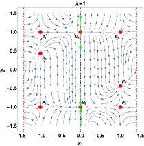
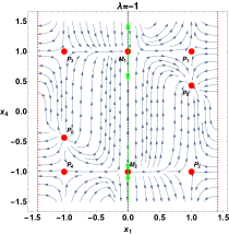
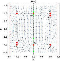
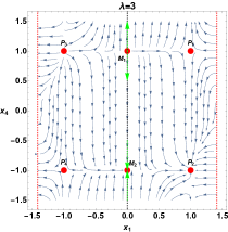
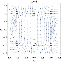
Figure 1: Phase-space plots for system (34)-(35) for the values $\lambda=1,\pm 2,\pm 3$. The black dotted line is the manifold for points $M_{1,2}$. The red dotted lines correspond to the vertical line $x_{=}\pm\sqrt{2}$. These lines are the singularities previously mentioned in which the direction of the flow changes.

Label	$(x_{1},x_{4})$	$(x_{2},x_{3})$	Attractor?	Acceleration?	Interpretation
$P_{1}$	$(1,1)$	$(0,0)$	Yes*	No, $q=3$	Super-collapse
$P_{2}$	$(1,-1)$	$(0,0)$	Yes*	No, $q=3$	Super-collapse
$P_{3}$	$(-1,1)$	$(0,0)$	No	No, $q=3$	Super-collapse
$P_{4}$	$(-1,-1)$	$(0,0)$	No	No, $q=3$	Super-collapse
$P_{5}$	$(1,-\frac{\sqrt{3}\lambda}{4})$	$\left(0,\sqrt{1-\frac{3\lambda^{2}}{16}}\right)$	Yes	Yes, $q=-1+\frac{3\lambda^{2}}{4}$	Scaling solution
$P_{6}$	$(-1,\frac{\sqrt{3}\lambda}{4})$	$\left(0,\sqrt{1-\frac{3\lambda^{2}}{16}}\right)$	No	Yes, $q=-1+\frac{3\lambda^{2}}{4}$	Scaling solution
$M_{1}$	$(0,1)$	$(1,0)$	No	No, $q=1$	decelerated
$M_{2}$	$(0,-1)$	$(1,0)$	No	No, $q=1$	decelerated

Table 1: Summary of the analysis of system (34)-(35). The $x_{3}$ coordinate gives the interval of existence for $P_{5,6}$. The asterisk indicates that we can restrict the parameter $\lambda$ if we do not wish to have a super-collapse solution as a late-time attractor (see Theorem 2 and the comment after it.

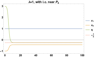
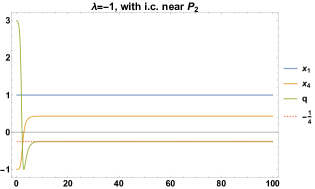
Figure 2: Numerical solution for system (34)-(35) for $\lambda=\pm 1$ and initial conditions near the point $P_{2}$ with a displacement of $\xi=10^{-3}$. In both cases, $P_{2}$ is a saddle point, which means that the system initially near $P_{2}$ will converge into the nearest attractor, in this case, $P_{5}$ with coordinates $x_{1}=1$ and $x_{4}=-\sqrt{3}/4$. Also, the deceleration parameter is depicted as a green line in the plots. For both values of $\lambda$, we see that after an initially decelerated stage, the solution accelerates into the scaling solution for $q(P_{5})\to-1/4$. However, for $\lambda=-1$, we see that there is an intermediate accelerated behaviour after the initial super-collapsing stage and before the scaling solution regime since $q$ reaches the de Sitter value $-1$.

III.1.2 Alternative formulation for the constant coupling function model

This section presents an alternative dynamical system formulation for the constant coupling function of section III.1.1. Since the constraints (27) describe two circumferences, we choose a reparametrization in polar coordinates as follows

$$x_{1}=\cos(\theta_{1}),\quad x_{2}=\sin(\theta_{1}),\quad x_{3}=\cos(\theta_{2}),\quad x_{4}=\sin(\theta_{2}).$$ (37)

With (37), we define the new variables for the dynamical systems analysis

$$\theta_{1}=\arctan\left(\frac{x_{2}}{x_{1}}\right)=\arctan(2\sqrt{\alpha}H)\quad\text{and}\quad\theta_{2}=\arctan\left(\frac{x_{4}}{x_{3}}\right)=\arctan\left(\frac{\dot{\phi}}{\sqrt{2}\sqrt{V(\phi)}}\right).$$ (38)

With inverse transformation given by

$$H=\frac{\tan(\theta_{1})}{2\sqrt{\alpha}},\quad\dot{\phi}=\sqrt{2}\tan(\theta_{2})\sqrt{V(\phi)}$$ (39)

Using the definition (38) and setting $\tau=\ln(a)$ we obtain the following two-dimensional system of first-order differential equations

$$\frac{d\theta_{1}}{d\tau} =\frac{4\sin(\theta_{1})\cos^{2}(\theta_{1})\sin^{2}(\theta_{2})}{\sqrt{3}(\cos(2\theta_{1})-3)},$$ (40)

$$\frac{d\theta_{2}}{d\tau} =-\frac{1}{6}\cos(\theta_{2})\left(4\sqrt{3}\cos(\theta_{1})\sin(\theta_{2})+3\lambda\right).$$ (41)

From equations (39), we remark that for $H$ to be continuous and simply so that the inverse transformations are defined, we must restrict the angles $\theta_{1,2}$ to $(-\frac{\pi}{2},\frac{\pi}{2})$. The equilibrium points for (40)-(41) are periodic, but we will consider the following ranges $\theta_{1}\in[-\pi,\pi]$ and $\theta_{2}\in[-\pi,\pi]$, this choice will allow us to transfer from one branch of the solutions to the other one. Considering $c_{1},c_{2}\in\mathbb{Z}$, the equilibrium points for system (40)-(41) are

1. $T_{1}=(2\pi c_{1},2\pi c_{2}+\frac{\pi}{2})$,

2. $T_{2}=(2\pi c_{1},2\pi c_{2}-\frac{\pi}{2})$,

3. $T_{3}=(2\pi c_{1}-\frac{\pi}{2},2\pi c_{2}+\frac{\pi}{2})$,

4. $T_{4}=(2\pi c_{1}-\frac{\pi}{2},2\pi c_{2}-\frac{\pi}{2})$,

5. $T_{5}=(2\pi c_{1}+\frac{\pi}{2},2\pi c_{2}-\frac{\pi}{2})$,

6. $T_{6}=(2\pi c_{1}+\frac{\pi}{2},2\pi c_{2}+\frac{\pi}{2})$,

7. $T_{7}=(2\pi c_{1}+\pi,2\pi c_{2}+\frac{\pi}{2})$,

8. $T_{8}=(2\pi c_{1}+\pi,2\pi c_{2}-\frac{\pi}{2})$,

9. $T_{9}=(2\pi c_{1},\tan^{-1}\left(\sqrt{48-9\lambda^{2}},-3\lambda\right)+2\pi c_{2})$,

10. $T_{10}=(2\pi c_{1},\tan^{-1}\left(-\sqrt{48-9\lambda^{2}},-3\lambda\right)+2\pi c_{2})$,

11. $T_{11}=(2\pi c_{1}+\pi,\tan^{-1}\left(\sqrt{48-9\lambda^{2}},3\lambda\right)+2\pi c_{2})$,

12. $T_{12}=(2\pi c_{1}+\pi,\tan^{-1}\left(-\sqrt{48-9\lambda^{2}},3\lambda\right)+2\pi c_{2})$.

We have used the notation $\tan^{-1}(x,y)=\tan^{-1}\left(\frac{y}{x}\right)$. The first eight points lie within the previously mentioned range for $c_{1}=c_{2}=0$. Additionally, points seven and eight can have $c_{1}=-1$. Points nine and ten also require $c_{1}=0$ and additionally $\frac{-\tan^{-1}\left(\pm\sqrt{48-9\lambda^{2}},-3\lambda\right)-\pi}{2\pi}\leq c_{2}\leq\frac{\pi-\tan^{-1}\left(\pm\sqrt{48-9\lambda^{2}},-3\lambda\right)}{2\pi}$. The last two points are in the desired range for $c_{1}=0$ or $c_{1}=-1$ and $\frac{-\tan^{-1}\left(\pm\sqrt{48-9\lambda^{2}},-3\lambda\right)-\pi}{2\pi}\leq c_{2}\leq\frac{\pi-\tan^{-1}\left(\pm\sqrt{48-9\lambda^{2}},-3\lambda\right)}{2\pi}$. To illustrate the relationship between these points and the ones from section III.1.1, taking into consideration the values of $\lambda$ used to plot the dynamics, we will consider only $c_{1}=c_{2}=0$ and $c_{1}=-1$, $c_{2}=0$.

In Table 2, we present the selected equilibrium points and their corresponding counterparts of section III.1.1. We chose some values for the constants $c_{1,2}$ that appear because of the periodicity of the trigonometric functions. These choices ensure that the equilibrium points lie in the desired range. For the plots presented in the following figures, we use the labels of the points from section III.1.1. In figures 3 and 4, we depict the two-dimensional phase portraits for system (40)-(41) for different values of the parameter $\lambda$. Recall that under this alternative formulation, the physical region is highlighted inside the dashed-orange square $(-\frac{\pi}{2},\frac{\pi}{2}),\times(-\frac{\pi}{2},\frac{\pi}{2})$. On the other hand, the vertical black lines correspond to the values where the tangent function in equation (39) is not defined.

In figure 5 the dynamics of system (40)-(41) is depicted as “wrapped” around a torus given by the parametrization $x=(R+r\cos(\theta_{1}-\pi))\cos(\theta_{2}-\pi),\quad y=(R+r\cos(\theta_{1}-\pi))\sin(\theta_{2}-\pi)$, and $z=r\sin(\theta_{1}-\pi)$ for $r=1$ and $R=3$. We are motivated to present our results this way because the original variables $x_{i}$ lie within two circumferences defined by the constraint (27). One is represented by the angle $\theta_{1}$ and the other by $\theta_{2}$, the poloidal and toroidal directions of the torus. In figure 6 we present some numerical solutions of system (40)-(41) for two values of the parameter $\lambda=1,-3$ and initial conditions near $P_{2}$ displacement of $\xi=10^{-3}$. A possible model evolution can be determined by analysing the behaviour of the deceleration parameter, depicted as a green line. For $\lambda=1$, we see that after an initial decelerated stage, the solution accelerates to $q(P_{5})\rightarrow-\frac{1}{4}$, the scaling solution. For $\lambda=-3$, the solution is decelerated since $q\rightarrow 3$ but has a brief accelerated stage when $q<0$.

Label	$(\theta_{1},\theta_{2})$	$c_{1},c_{2}$	Sect. III.1.1 point
$T_{1}$	$(0,\frac{\pi}{2})$	$0,0$	$P_{1}$
$T_{2}$	$(0,-\frac{\pi}{2})$	$0,0$	$P_{2}$
$T_{3}$	$\left(\frac{\pi}{2},\frac{\pi}{2}\right)$	$0,0$	$M_{1}$
$T_{4}$	$\left(-\frac{\pi}{2},\frac{\pi}{2}\right)$	$0,0$	Symmetric to $M_{1}$
$T_{5}$	$\left(\frac{\pi}{2},-\frac{\pi}{2}\right)$	$0,0$	$M_{2}$
$T_{6}$	$\left(-\frac{\pi}{2},-\frac{\pi}{2}\right)$	$0,0$	Symmetric to $M_{2}$
$T_{7}$	$\left(\pi,\frac{\pi}{2}\right)$	$0,0$	$P_{3}$
$T_{7}*$	$\left(-\pi,\frac{\pi}{2}\right)$	$-1,0$	$P_{3}$
$T_{8}$	$\left(\pi,-\frac{\pi}{2}\right)$	$0,0$	$P_{4}$
$T_{8}*$	$\left(-\pi,-\frac{\pi}{2}\right)$	$-1,0$	$P_{4}$
$T_{9}$	$\left(0,\tan^{-1}\left(\sqrt{48-9\lambda^{2}},-3\lambda\right)\right)$	$0,0$	$P_{5}$
$T_{10}$	$\left(0,\tan^{-1}\left(-\sqrt{48-9\lambda^{2}},-3\lambda\right)\right)$	$0,0$	Symmetric to $P_{5}$
$T_{11}$	$\left(\pi,\tan^{-1}\left(\sqrt{48-9\lambda^{2}},3\lambda\right)\right)$	$0,0$	$P_{6}$
$T_{11}*$	$\left(-\pi,\tan^{-1}\left(\sqrt{48-9\lambda^{2}},3\lambda\right)\right)$	$-1,0$	$P_{6}$
$T_{12}$	$\left(\pi,\tan^{-1}\left(-\sqrt{48-9\lambda^{2}},3\lambda\right)\right)$	$0,0$	Symmetric to $P_{6}$
$T_{12}*$	$\left(-\pi,\tan^{-1}\left(-\sqrt{48-9\lambda^{2}},3\lambda\right)\right)$	$-1,0$	Symmetric to $P_{6}$

Table 2: Summary of the equilibrium points of system (40)-(41). The corresponding points from section III.1.1 are derived by applying the definitions in equation (37). The asterisk next to some points means a different choice of $c_{1}$ was made from the original list. For every point, the stability analysis and the value of the deceleration parameter are the same as in section III.1.1.

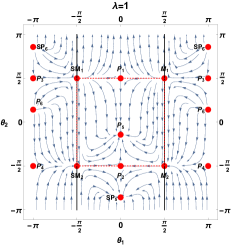
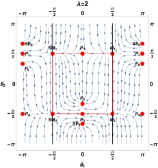
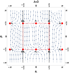
Figure 3: Phase plane analysis for system (40)-(41) for the values $\lambda=1,2,3$. The physical region under this formulation is the inside of the orange square. We labelled the points according to the corresponding points in section III.1.1. The points with different labels like $SM_{1}$ represent symmetric points that were not present In the original analysis because of the constraints on the $x_{i}$ variables. The black vertical lines correspond to the values $\pm\frac{\pi}{2}$ where the inverse transformations are not defined.

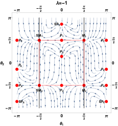
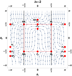
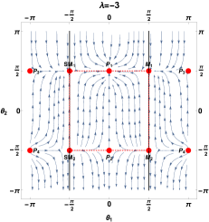
Figure 4: Phase plane analysis for system (40)-(41) for the values $\lambda=-1,-2,-3$. The physical region under this formulation is the inside of the orange square. We labelled the points according to the corresponding points in section III.1.1. The points with different labels like $SM_{1}$ represent symmetric points that were not present In the original analysis because of the constraints on the $x_{i}$ variables. The black vertical lines correspond to the values $\pm\frac{\pi}{2}$ where the inverse transformations are not defined.

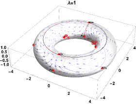
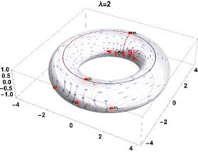
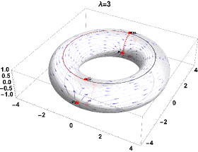
Figure 5: Dynamics of system (40)-(41) in the surface of a torus using the following parametrization $x=(R+r\cos(\theta_{1}-\pi))\cos(\theta_{2}-\pi),\quad x=(R+r\cos(\theta_{1}-\pi))\sin(\theta_{2}-\pi)$, and $z=r\sin(\theta_{1}-\pi)$ for $r=1$ and $R=3$. We have considered $\theta_{1}$ and $\theta_{2}$ as the poloidal and toroidal directions. As the 2-dimensional phase plots of Fig. 3 wrap around the torus, we can transfer from one branch to another. The values $\lambda=1,2,3$ were considered noting that in figure 3 the dynamic for the negative values is symmetrical.

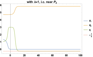
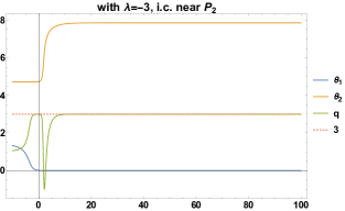
Figure 6: Numerical solutions of system (40)-(41) for different values of the parameter $\lambda=1,-3$ and initial conditions near $P_{2}$ displacement of $\xi=10^{-3}$. Also in the plots, the deceleration parameter is depicted as a green line. For $\lambda=1$, we see that after an initial decelerated stage, the solution accelerates to $q(P_{5})\rightarrow-\frac{1}{4}$, the scaling solution. For $\lambda=-3$, the solution is a decelerated one since $q\rightarrow 3$ but has a brief accelerated stage when $q<0$.

III.2 Linear coupling function: $f(\phi)=-\alpha\phi$

In this section, we define the coupling between the scalar function and the Gauss-Bonnet term as a linear function $f(\phi)=-\alpha\phi$. Hence, the field equations are

$$12H^{2}\left(4\alpha\phi\dot{H}+4\alpha\ddot{\phi}+1\right)+96\alpha H\dot{H}\dot{\phi}+6\dot{H}+144\alpha H^{3}\dot{\phi}+48\alpha H^{4}\phi-2V(\phi)+\dot{\phi}^{2}= 0,$$ (42)

$$96\alpha H^{2}\dot{H}+120\alpha H^{4}-4H\dot{\phi}-V^{\prime}(\phi)-\ddot{\phi}= 0.$$ (43)

We can also write Friedmann’s equation (17) as

$$96\alpha H^{3}\dot{\phi}+24\alpha H^{4}\phi+6H^{2}=V(\phi)+\frac{1}{2}\dot{\phi}^{2},$$ (44)

and the deceleration parameter as

$$q=-1-\frac{\dot{H}}{H^{2}}=\frac{-144\alpha H^{3}\dot{\phi}+6H^{2}\left(192\alpha^{2}H^{4}-8\alpha\lambda V(\phi)+1\right)-2V(\phi)+\dot{\phi}^{2}}{6H^{2}\left(8\alpha H\left(96\alpha H^{3}+H\phi+2\dot{\phi}\right)+1\right)}.$$ (45)

III.2.1 Dynamical system analysis for linear $f$

We can define $\chi=V(\phi)+\frac{1}{2}\dot{\phi}^{2}$ as before and define the following dimensionless variables

$$x_{1}=\frac{\sqrt{6}H}{\sqrt{\chi}},\quad x_{2}=\frac{2\sqrt{6}\sqrt{\alpha H^{4}\phi}}{\sqrt{\chi}},\quad x_{3}=\frac{\sqrt{V(\phi)}}{\sqrt{\chi}},\quad x_{4}=\frac{\dot{\phi}}{\sqrt{2}\sqrt{\chi}},\quad x_{5}=\frac{4\sqrt{6}\sqrt{\alpha H^{3}}}{\sqrt[4]{\chi}},$$ (46)

with inverse transformation given by

$$H=\frac{x_{1}\sqrt{\chi}}{\sqrt{6}},\quad\phi=\frac{4\sqrt{6}x_{2}^{2}}{x_{1}x_{5}^{2}},\quad V(\phi)=x_{3}^{2}\chi,\quad\dot{\phi}=\sqrt{2}x_{4}\sqrt{\chi},\quad\alpha=\frac{\sqrt{\frac{3}{2}}x_{5}^{2}}{8x_{1}^{3}\chi}.$$ (47)

By replacing these variables in (44), we obtain the following restrictions

$$x_{1}^{2}+x_{2}^{2}+\sqrt{2}x_{4}x_{5}^{2}=1,\quad x_{3}^{2}+x_{4}^{2}=1,$$ (48)

we also have the following ranges for the new variables $0\leq x_{2}$, $0\leq x_{3}\leq 1$, $-1\leq x_{4}\leq 1$, $0\leq x_{5}$. With this, we can write the following five-dimensional dynamical system

$$x_{1}^{\prime} =\frac{x_{1}\left(x_{1}^{3}\left(32x_{4}^{2}+3\sqrt{2}x_{4}x_{5}^{2}-16\right)+x_{1}\left(-2\sqrt{2}x_{4}x_{5}^{2}\left(x_{2}^{2}+4x_{3}^{2}-2\right)+2x_{4}^{2}\left(32x_{2}^{2}+x_{5}^{4}-8\right)\right)\right)}{4\sqrt{6}\left(2x_{1}^{2}+4x_{2}^{2}+2\sqrt{2}x_{4}x_{5}^{2}+x_{5}^{4}\right)}$$ (49)

$$+\frac{x_{1}\left(-16x_{2}^{2}+16x_{3}^{2}+40\sqrt{2}x_{4}^{3}x_{5}^{2}-5x_{5}^{4}\right)+4\sqrt{3}\lambda x_{3}^{2}x_{5}^{2}\left(\sqrt{2}-x_{4}x_{5}^{2}\right)}{4\sqrt{6}\left(2x_{1}^{2}+4x_{2}^{2}+2\sqrt{2}x_{4}x_{5}^{2}+x_{5}^{4}\right)}$$

$$x_{2}^{\prime} =\frac{2x_{1}^{3}\left(16\sqrt{2}x_{2}^{2}\left(x_{4}^{2}-1\right)+\left(3x_{2}^{2}+1\right)x_{4}x_{5}^{2}\right)-4\sqrt{3}\lambda x_{2}^{2}x_{3}^{2}x_{5}^{2}\left(\sqrt{2}x_{4}x_{5}^{2}-4\right)}{8\sqrt{3}x_{2}\left(2x_{1}^{2}+4x_{2}^{2}+2\sqrt{2}x_{4}x_{5}^{2}+x_{5}^{4}\right)}$$ (50)

$$+\frac{x_{1}\left(-4x_{2}^{2}x_{4}x_{5}^{2}\left(x_{2}^{2}+4x_{3}^{2}-20x_{4}^{2}-5\right)+32\sqrt{2}x_{2}^{2}\left(\left(2x_{2}^{2}-1\right)x_{4}^{2}-x_{2}^{2}+x_{3}^{2}\right)+2\sqrt{2}x_{5}^{4}\left(x_{2}^{2}\left(x_{4}^{2}-5\right)+x_{4}^{2}\right)+x_{4}x_{5}^{6}\right)}{8\sqrt{3}x_{2}\left(2x_{1}^{2}+4x_{2}^{2}+2\sqrt{2}x_{4}x_{5}^{2}+x_{5}^{4}\right)}$$

$$x_{3}^{\prime} =\frac{x_{3}x_{4}\left(x_{1}^{3}\left(32\sqrt{3}x_{4}+3\sqrt{6}x_{5}^{2}\right)+24\lambda x_{1}^{2}+2\sqrt{3}x_{1}\left(x_{2}^{2}\left(32x_{4}-\sqrt{2}x_{5}^{2}\right)-4\sqrt{2}x_{5}^{2}\left(x_{3}^{2}-5x_{4}^{2}\right)+x_{4}x_{5}^{4}\right)\right)}{12\sqrt{2}\left(2x_{1}^{2}+4x_{2}^{2}+2\sqrt{2}x_{4}x_{5}^{2}+x_{5}^{4}\right)}$$ (51)

$$+\frac{x_{3}x_{4}\left(12\lambda\left(4x_{2}^{2}-x_{3}^{2}x_{5}^{4}+2\sqrt{2}x_{4}x_{5}^{2}+x_{5}^{4}\right)\right)}{12\sqrt{2}\left(2x_{1}^{2}+4x_{2}^{2}+2\sqrt{2}x_{4}x_{5}^{2}+x_{5}^{4}\right)}$$

$$x_{4}^{\prime} =\frac{\sqrt{3}x_{1}^{3}\left(x_{4}^{2}-1\right)\left(32x_{4}+3\sqrt{2}x_{5}^{2}\right)-12\lambda x_{3}^{2}\left(4x_{2}^{2}+x_{4}x_{5}^{2}\left(x_{4}x_{5}^{2}+2\sqrt{2}\right)\right)}{12\sqrt{2}\left(2x_{1}^{2}+4x_{2}^{2}+2\sqrt{2}x_{4}x_{5}^{2}+x_{5}^{4}\right)}$$ (52)

$$+\frac{-24\lambda x_{1}^{2}x_{3}^{2}+2\sqrt{3}x_{1}\left(x_{4}^{2}-1\right)\left(x_{2}^{2}\left(32x_{4}-\sqrt{2}x_{5}^{2}\right)-4\sqrt{2}x_{5}^{2}\left(x_{3}^{2}-5x_{4}^{2}\right)+x_{4}x_{5}^{4}\right)}{12\sqrt{2}\left(2x_{1}^{2}+4x_{2}^{2}+2\sqrt{2}x_{4}x_{5}^{2}+x_{5}^{4}\right)}$$

$$x_{5}^{\prime} =\frac{16x_{1}x_{5}\left(x_{4}^{2}\left(2x_{1}^{2}+4x_{2}^{2}-3\right)-3\left(x_{1}^{2}+x_{2}^{2}-x_{3}^{2}\right)\right)+x_{5}^{5}\left(x_{1}\left(2x_{4}^{2}-15\right)-4\sqrt{3}\lambda x_{3}^{2}x_{4}\right)}{8\sqrt{6}\left(2x_{1}^{2}+4x_{2}^{2}+2\sqrt{2}x_{4}x_{5}^{2}+x_{5}^{4}\right)}$$ (53)

$$+\frac{16x_{1}x_{5}\left(x_{4}^{2}\left(2x_{1}^{2}+4x_{2}^{2}-3\right)-3\left(x_{1}^{2}+x_{2}^{2}-x_{3}^{2}\right)\right)+x_{5}^{5}\left(x_{1}\left(2x_{4}^{2}-15\right)-4\sqrt{3}\lambda x_{3}^{2}x_{4}\right)}{8\sqrt{6}\left(2x_{1}^{2}+4x_{2}^{2}+2\sqrt{2}x_{4}x_{5}^{2}+x_{5}^{4}\right)}.$$

In these variables, the deceleration parameter (45) reads

$$q=\frac{8x_{1}^{3}+x_{1}\left(-16x_{3}^{2}+16x_{4}^{2}-12\sqrt{2}x_{4}x_{5}^{2}+x_{5}^{4}\right)-4\sqrt{6}\lambda x_{3}^{2}x_{5}^{2}}{4x_{1}\left(2x_{1}^{2}+4x_{2}^{2}+2\sqrt{2}x_{4}x_{5}^{2}+x_{5}^{4}\right)}$$ (54)

We can use the restrictions (48) together with the fact that $x_{2}\geq 0$ and $x_{3}\geq 0$ to obtain the following positive roots

$$x_{2}=\sqrt{-x_{1}^{2}-\sqrt{2}x_{4}x_{5}^{2}+1},\quad x_{3}=\sqrt{1-x_{4}^{2}}$$ (55)

provided $x_{1}^{2}+\sqrt{2}x_{4}x_{5}^{2}\leq 1$.

With these definitions, we can obtain the following reduced three-dimensional dynamical system

$$x_{1}^{\prime} =\frac{x_{1}\left(\sqrt{2}x_{5}^{2}\left(-5x_{1}^{3}x_{4}+2x_{1}x_{4}\left(8x_{4}^{2}-5\right)+4\sqrt{3}\lambda\left(x_{4}^{2}-1\right)\right)+32x_{1}\left(x_{1}^{2}-1\right)x_{4}^{2}+x_{5}^{4}\left(x_{1}\left(5-6x_{4}^{2}\right)-4\sqrt{3}\lambda x_{4}\left(x_{4}^{2}-1\right)\right)\right)}{4\sqrt{6}\left(2x_{1}^{2}+2\sqrt{2}x_{4}x_{5}^{2}-x_{5}^{4}-4\right)},$$ (56)

$$x_{4}^{\prime} =\frac{\left(x_{4}^{2}-1\right)\left(x_{1}^{3}\left(32\sqrt{3}x_{4}-5\sqrt{6}x_{5}^{2}\right)+24\lambda x_{1}^{2}+2\sqrt{3}x_{1}\left(\sqrt{2}\left(8x_{4}^{2}+5\right)x_{5}^{2}-3x_{4}x_{5}^{4}-32x_{4}\right)+12\lambda\left(-x_{4}^{2}x_{5}^{4}+2\sqrt{2}x_{4}x_{5}^{2}-4\right)\right)}{12\sqrt{2}\left(2x_{1}^{2}+2\sqrt{2}x_{4}x_{5}^{2}-x_{5}^{4}-4\right)},$$ (57)

$$x_{5}^{\prime} =\frac{\sqrt{2}x_{5}^{3}\left(5x_{1}^{3}x_{4}+2x_{1}x_{4}\left(25-8x_{4}^{2}\right)-12\sqrt{3}\lambda\left(x_{4}^{2}-1\right)\right)-32x_{1}\left(x_{1}^{2}+1\right)x_{4}^{2}x_{5}+x_{5}^{5}\left(3x_{1}\left(2x_{4}^{2}-5\right)+4\sqrt{3}\lambda x_{4}\left(x_{4}^{2}-1\right)\right)}{8\sqrt{6}\left(-2x_{1}^{2}-2\sqrt{2}x_{4}x_{5}^{2}+x_{5}^{4}+4\right)}.$$ (58)

Using (45) and (55) deceleration parameter is

$$q=-\frac{8x_{1}^{3}+x_{1}\left(32x_{4}^{2}-12\sqrt{2}x_{4}x_{5}^{2}+x_{5}^{4}-16\right)+4\sqrt{6}\lambda\left(x_{4}^{2}-1\right)x_{5}^{2}}{4x_{1}\left(2x_{1}^{2}+2\sqrt{2}x_{4}x_{5}^{2}-x_{5}^{4}-4\right)}.$$ (59)

From equations (54) and (59), we see that the deceleration parameter is not defined for $x_{1}=0$, but we can still study its limit as $x_{1}\rightarrow 0$ for the equilibrium points where $x_{1}=0$. The equilibrium points for system (56)-(58) are

1. The normally hyperbolic family $F_{1}=(\frac{4\sqrt{6}\lambda}{x_{5_{c}}^{2}},0,x_{5_{c}})$. This family exists for $x_{5_{c}}>0,-\frac{5\sqrt{x_{5_{c}}^{4}}}{4\sqrt{6}}<\lambda<\frac{5\sqrt{x_{5_{c}}^{4}}}{4\sqrt{6}}$. The eigenvalues are $\{0,\frac{1536\lambda^{3}-200\lambda\left(x_{5_{c}}^{4}+4\right)x_{5_{c}}^{4}-2\sqrt{\lambda^{2}\left(25x_{5_{c}}^{4}\left(x_{5_{c}}^{4}+4\right)-192\lambda^{2}\right)\left(-3072\lambda^{2}+275x_{5_{c}}^{8}+400\left(3\lambda^{2}+4\right)x_{5_{c}}^{4}\right)}}{125x_{5_{c}}^{6}\left(x_{5_{c}}^{4}+4\right)-960\lambda^{2}x_{5_{c}}^{2}},\\ \frac{2\left(768\lambda^{3}-100\lambda\left(x_{5_{c}}^{4}+4\right)x_{5_{c}}^{4}+\sqrt{\lambda^{2}\left(25x_{5_{c}}^{4}\left(x_{5_{c}}^{4}+4\right)-192\lambda^{2}\right)\left(-3072\lambda^{2}+275x_{5_{c}}^{8}+400\left(3\lambda^{2}+4\right)x_{5_{c}}^{4}\right)}\right)}{125x_{5_{c}}^{6}\left(x_{5_{c}}^{4}+4\right)-960\lambda^{2}x_{5}^{2}}\}$, see Fig. 7 for a representation of the real part of the nonzero eigenvalues. The nonzero eigenvalues determine the stability of the family. The family is

   1. an attractor for $\lambda>0,\sqrt{15}x_{5_{c}}^{2}>12\lambda$,

   2. a source for $-\frac{1}{4}\sqrt{\frac{5}{3}}x_{5_{c}}^{2}<\lambda<0$,

   3. a saddle for $-\frac{5x_{5_{c}}^{2}}{4\sqrt{6}}<\lambda<-\frac{1}{4}\sqrt{\frac{5}{3}}x_{5_{c}}^{2}$ or $\frac{1}{4}\sqrt{\frac{5}{3}}x_{5_{c}}^{2}<\lambda<\frac{5x_{5_{c}}^{2}}{4\sqrt{6}}$,

   4. non-hyperbolic for $\lambda=0$ or $12\lambda+\sqrt{15}x_{5_{c}}^{2}=0$ or $\sqrt{15}x_{5_{c}}^{2}=12\lambda$.

      

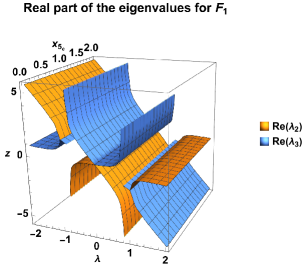
      Figure 7: Real part of the eigenvalues for the normally hyperbolic family of points $F_{1}$. Here we see $\lambda_{2}$ and $\lambda_{3}$ the nonzero eigenvalues.

      We also verify that $q(F_{1})=-1$, , which means that the family describes a de Sitter solution.

2. The normally hyperbolic family $L_{1}=(0,1,x_{5_{c}})$ has eigenvalues $\{0,0,\sqrt{2}\lambda\}$. This family exists for $0\leq x_{5_{c}}\leq\frac{1}{\sqrt[4]{2}}$ and is unstable for $\lambda>0$ and stable for $\lambda<0$. Since $x_{1}=0$, we study $q$ as $x_{1}\rightarrow 0$, this means that $\lim_{x_{1}\rightarrow 0}q(L_{1})=\frac{x_{5_{c}}^{4}-12\sqrt{2}x_{5_{c}}^{2}+16}{4x_{5_{c}}^{4}-8\sqrt{2}x_{5_{c}}^{2}+16}$. This means that $L_{1}$ cannot describe an accelerated solution since $0\leq\frac{x_{5_{c}}^{4}-12\sqrt{2}x_{5_{c}}^{2}+16}{4x_{5_{c}}^{4}-8\sqrt{2}x_{5_{c}}^{2}+16}\leq 1$.

3. The normally hyperbolic family $L_{2}=(0,-1,x_{5_{c}})$ has eigenvalues $\{0,0,-\sqrt{2}\lambda\}$. This family exists for $x_{5_{c}}\geq 0$ and is unstable for $\lambda<0$ and stable for $\lambda>0$. Since $x_{1}=0$, we study $q$ as $x_{1}\rightarrow 0$, this means that $\lim_{x_{1}\rightarrow 0}q(L_{1})=\frac{-x_{5_{c}}^{4}+12\sqrt{2}x_{5_{c}}^{2}-16}{-4x_{5_{c}}^{4}+8\sqrt{2}x_{5_{c}}^{2}-16}$. This means that $L_{2}$ describes an accelerated solution for $\sqrt{2\left(3\sqrt{2}-\sqrt{14}\right)}<x_{5_{c}}<\sqrt{2\left(3\sqrt{2}+\sqrt{14}\right)}$

4. $Q_{1}=(1,1,0)$, with eigenvalues $\left\{-4\sqrt{\frac{2}{3}},-2\sqrt{\frac{2}{3}},\frac{1}{3}\sqrt{2}\left(3\lambda+4\sqrt{3}\right)\right\}$. This point is

   1. an attractor for for $\lambda<-\frac{4}{\sqrt{3}}$,

   2. a saddle for $\lambda>-\frac{4}{\sqrt{3}}$,

   3. non-hyperbolic for $\lambda=-\frac{4}{\sqrt{3}}$.

   We also verify that $Q_{1}$ describes a super-collapse solution because $q(Q_{1})=3$.

5. $Q_{2}=(1,-1,0)$, with eigenvalues $\left\{-4\sqrt{\frac{2}{3}},-2\sqrt{\frac{2}{3}},\frac{1}{3}\sqrt{2}\left(4\sqrt{3}-3\lambda\right)\right\}$. This point is

   1. an attractor for $\lambda>\frac{4}{\sqrt{3}}$,

   2. a saddle for $\lambda<\frac{4}{\sqrt{3}}$,

   3. non-hyperbolic for $\lambda=\frac{4}{\sqrt{3}}$.

   As before, $Q_{2}$ describes a super-collapse solution because $q(Q_{2})=3$.

6. $Q_{3}=(-1,1,0)$, with eigenvalues $\left\{4\sqrt{\frac{2}{3}},2\sqrt{\frac{2}{3}},\frac{1}{3}\sqrt{2}\left(3\lambda-4\sqrt{3}\right)\right\}$. This point is

   1. a source for $\lambda>\frac{4}{\sqrt{3}}$,

   2. a saddle for $\lambda<\frac{4}{\sqrt{3}}$,

   3. non-hyperbolic for $\lambda=\frac{4}{\sqrt{3}}$.

   We verify that $Q_{3}$ describes the same type of super-collapse solution as $Q_{1,2}$ because $q(Q_{3})=3$.

7. $Q_{4}=(-1,-1,0)$, with eigenvalues $\left\{4\sqrt{\frac{2}{3}},2\sqrt{\frac{2}{3}},\frac{1}{3}\sqrt{2}\left(-3\lambda-4\sqrt{3}\right)\right\}$. This point is

   1. a source for $\lambda<-\frac{4}{\sqrt{3}}$,

   2. a saddle for $\lambda>-\frac{4}{\sqrt{3}}$,

   3. non-hyperbolic for $\lambda=-\frac{4}{\sqrt{3}}$.

   As it was the case of $Q_{3}$, we observe that $q(Q_{4})=3$.

8. $Q_{5}=(1,-\frac{\sqrt{3}\lambda}{4},0)$, with eigenvalues $\left\{-\frac{1}{2}\sqrt{\frac{3}{2}}\lambda^{2},-\frac{1}{4}\sqrt{\frac{3}{2}}\lambda^{2},\frac{3\lambda^{2}-16}{4\sqrt{6}}\right\}$. This point exists for $-\frac{4}{\sqrt{3}}\leq\lambda\leq\frac{4}{\sqrt{3}}$ and is

   1. an attractor for $-\frac{4}{\sqrt{3}}<\lambda<0$ or $0<\lambda<\frac{4}{\sqrt{3}}$,

   2. non-hyperbolic for $\lambda=0$ or $\lambda=-\frac{4}{\sqrt{3}}$ or $\lambda=\frac{4}{\sqrt{3}}$.

   The deceleration parameter is $q(Q_{5})=-1+\frac{3\lambda^{2}}{4}$, which is a scaling solution. This means that $Q_{5}$ describes an accelerated solution for $-\frac{2}{\sqrt{3}}<\lambda<\frac{2}{\sqrt{3}}$. It describes a decelerated solution for $\lambda<-\frac{2}{\sqrt{3}}$ or $\lambda>\frac{2}{\sqrt{3}}$. Finally it describes a de Sitter solution for $\lambda=0$.

9. $Q_{6}=(-1,\frac{\sqrt{3}\lambda}{4},0)$, with eigenvalues $\left\{\frac{1}{4}\sqrt{\frac{3}{2}}\lambda^{2},\frac{1}{2}\sqrt{\frac{3}{2}}\lambda^{2},-\frac{3\lambda^{2}-16}{4\sqrt{6}}\right\}$. This point exists for $-\frac{4}{\sqrt{3}}\leq\lambda\leq\frac{4}{\sqrt{3}}$ and is

   1. a source for $-\frac{4}{\sqrt{3}}<\lambda<0$ or $0<\lambda<\frac{4}{\sqrt{3}}$,

   2. non-hyperbolic for $\lambda=0$ or $\lambda=-\frac{4}{\sqrt{3}}$ or $\lambda=\frac{4}{\sqrt{3}}$.

   This point describes the same type of solutions as $Q_{5}$ since $q(Q_{6})=-1+\frac{3\lambda^{2}}{4}$.

In Table 3, we present a summary of the results of this section. Figures 8 and 9 depict different phase-plots for system (56)-(58) for different values of the parameter $\lambda$. We used $\lambda=\frac{1}{12}$ in order to confirm the attracting stability of the $F_{1}$ family of equilibrium points. In figure 10 we present a possible late-time evolution for system (56) -(58) for different values of $\lambda$ with initial conditions near $Q_{2}$ with a displacement of $\xi=10^{-3}$. Also, in the plots, the deceleration parameter is depicted as a red line. For both values of $\lambda$, we see that after an initially super-collapsing stage, the solution accelerates into one of the following two cases: towards the family $F_{1}$ since $q\rightarrow-1;$ towards the scaling solution $Q_{5}$ for which $q\rightarrow-\frac{1}{4}$. As in the previous section, we can write our findings in the following results

Theorem 3.

The late-time attractors for the five-dimensional Gauss-Bonnet model with linear coupling function are

1. The normally hyperbolic family $F_{1}=(\frac{4\sqrt{6}\lambda}{x_{5_{c}}^{2}},0,x_{5_{c}})$ for $\lambda>0,\sqrt{15}x_{5_{c}}^{2}>12\lambda$.

2. The normally hyperbolic family $L_{1}=(0,1,x_{5_{c}})$ for $\lambda<0$.

3. The normally hyperbolic family $L_{2}=(0,-1,x_{5_{c}})$ for $\lambda>0$.

4. The super-collapse solution $Q_{1}=(1,1,0)$ for $\lambda<-\frac{4}{\sqrt{3}}$.

5. The super-collapse solution $Q_{2}=(1,-1,0)$ for $\lambda>\frac{4}{\sqrt{3}}$.

6. The scaling solution $Q_{5}=(1,-\frac{\sqrt{3}\lambda}{4},0)$ for $-\frac{4}{\sqrt{3}}<\lambda<0$ or $0<\lambda<\frac{4}{\sqrt{3}}$.

As before, to avoid having super-collapsing solutions as late-time attractors for this model, we can restrict the numerical range for the parameter $\lambda$ in the range $-\frac{4}{\sqrt{3}}<\lambda<0$ or $0<\lambda<\frac{4}{\sqrt{3}}$. That modifies the region of parameters for some of the equilibrium points. We formulate this in the following result

Corollary 2.

The late-time attractors for the five-dimensional Gauss-Bonnet model with linear coupling function in the range $-\frac{4}{\sqrt{3}}<\lambda<0$ or $0<\lambda<\frac{4}{\sqrt{3}}$ are

1. The normally hyperbolic family $F_{1}=(\frac{4\sqrt{6}\lambda}{x_{5_{c}}^{2}},0,x_{5_{c}})$ for $0<\lambda<\frac{4}{\sqrt{3}},\sqrt{15}x_{5_{c}}^{2}>12\lambda.$

2. The normally hyperbolic family $L_{1}=(0,1,x_{5_{c}})$ for $-\frac{4}{\sqrt{3}}<\lambda<0.$

3. The normally hyperbolic family $L_{2}=(0,-1,x_{5_{c}})$ for $0<\lambda<\frac{4}{\sqrt{3}}.$

4. The scaling solution $Q_{5}=(1,-\frac{\sqrt{3}\lambda}{4},0)$ for $-\frac{4}{\sqrt{3}}<\lambda<0$ or $0<\lambda<\frac{4}{\sqrt{3}}$.

Notice that the late-time attractor for the model mentioned in the last item of corollary 2 corresponds to the sixth result in Theorem 3. Additionally, in section III.2.2, we study a projection of the three-dimensional dynamical system for linear coupling function to better visualise the dynamics for a fixed value of $x_{5_{c}}$ since the families $F_{1},L_{1},L_{2}$ depend on this free parameter.

Label	$(x_{1},x_{4},x_{5})$	$(x_{2},x_{3})$	Attractor?	Acceleration?	Interpretation
$F_{1}$	$\left(\frac{4\sqrt{6}\lambda}{5x_{5_{c}}^{2}},0,x_{5_{c}}\right)$	$\left(\sqrt{1-\frac{96\lambda^{2}}{25x_{5_{c}}^{4}}},1\right)$	Yes	Yes, $q=-1$	de Sitter
$L_{1}$	$\left(0,1,x_{5_{c}}\right)$	$\left(\sqrt{1-\sqrt{2}x_{5_{c}}},0\right)$	Yes	No, see text	decelerated
$L_{2}$	$(0,-1,x_{5_{c}})$	$\left(\sqrt{1+\sqrt{2}x_{5_{c}}},0\right)$	Yes	Yes, see text	accelerated
$Q_{1}$	$(1,1,0)$	$(0,0)$	Yes*	No, $q=3$	super-collapse
$Q_{2}$	$(1,-1,0)$	$(0,0)$	Yes*	No, $q=3$	super-collapse
$Q_{3}$	$(-1,1,0)$	$(0,0)$	No	No, $q=3$	super-collapse
$Q_{4}$	$(-1,-1,0)$	$(0,0)$	No	No, $q=3$	super-collapse
$Q_{5}$	$\left(1,-\frac{\sqrt{3}}{4}\lambda,0\right)$	$(0,\sqrt{1-\frac{3}{16}\lambda^{2}})$	Yes	Yes, $q=-1+\frac{3\lambda^{2}}{4}$	scaling solution
$Q_{6}$	$\left(1,\frac{\sqrt{3}}{4}\lambda,0\right)$	$(0,\sqrt{1-\frac{3}{16}\lambda^{2}})$	No	Yes, $q=-1+\frac{3\lambda^{2}}{4}$	scaling solution

Table 3: Summary of the analysis of system (56)-(58). The $x_{2}$ coordinate gives the interval of existence for the families $F_{1}$ and $L_{1,2}$. The $x_{3}$ coordinate gives the interval of existence for $Q_{5,6}$. The asterisk in $Q_{1,2}$ means that if we constrain the parameter $\lambda$, the super-collapse points would not be attractors for the model.

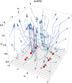
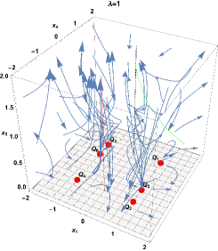
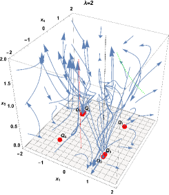
Figure 8: Dynamics of the three-dimensional system (56)-(58) for positive values of $\lambda$. The green-dashed curve corresponds to the family of equilibrium points $F_{1}$, we see that it is the attractor for $\lambda=\frac{1}{12}$. The black-dashed line represents the family $L_{1}$ and the red-dashed line represents the family $L_{2}$.

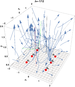
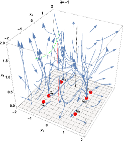
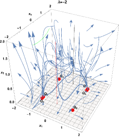
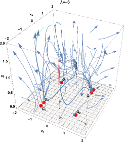
Figure 9: Dynamics of the three-dimensional system (56)-(58) for negative values of $\lambda$. The green-dashed curve corresponds to the family of equilibrium points $F_{1}$. The black-dashed line represents the family $L_{1}$ and the red-dashed line represents the family $L_{2}$. The behaviour is symmetric to that depicted in figure 8.

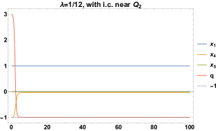
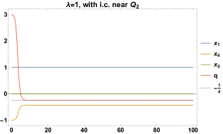
Figure 10: Possible late-time evolution for system (56) -(58) for different values of $\lambda$ with initial conditions near $Q_{2}$ with a displacement of $\xi=10^{-3}$. Also, in the plots, the deceleration parameter is depicted as a red line. For both values of $\lambda$, we see that after an initially super-collapsing stage, the solution accelerates into one of the following two cases: towards the family $F_{1}$ since $q\rightarrow-1;$ towards the scaling solution $Q_{5}$ for which $q\rightarrow-\frac{1}{4}$.

III.2.2 Two-dimensional projection of the dynamical system for linear coupling function

In the previous section, we obtained three families of equilibrium points that depend on the constant $x_{5}$. Now we wish to better observe the dynamics for a fixed value of $x_{5_{c}}$ so we consider a projection to $x_{5}=\mu$ in system (56)-(58) for $\mu\geq 0$.

Setting $x_{5}=\mu$ in system (56)-(58) and keeping the $x_{1}$ and $x_{4}$ equations we obtain

$$x_{1}^{\prime} =\frac{x_{1}\left(\sqrt{2}\mu^{2}\left(-5x_{1}^{3}x_{4}+2x_{1}x_{4}\left(8x_{4}^{2}-5\right)-\frac{x_{4}^{2}-1}{\sqrt{3}}\right)+32x_{1}\left(x_{1}^{2}-1\right)x_{4}^{2}+\mu^{4}\left(x_{1}\left(5-6x_{4}^{2}\right)+\frac{x_{4}\left(x_{4}^{2}-1\right)}{\sqrt{3}}\right)\right)}{4\sqrt{6}\left(-\mu^{4}+2x_{1}^{2}+2\sqrt{2}\mu^{2}x_{4}-4\right)},$$ (60)

$$x_{4}^{\prime} =\frac{\left(x_{4}^{2}-1\right)\left(\sqrt{3}x_{1}\left(-5\sqrt{2}\mu^{2}\left(x_{1}^{2}-2\right)+x_{4}\left(-6\mu^{4}+32x_{1}^{2}-64\right)+16\sqrt{2}\mu^{2}x_{4}^{2}\right)-2x_{1}^{2}+\mu^{4}x_{4}^{2}-2\sqrt{2}\mu^{2}x_{4}+4\right)}{12\sqrt{2}\left(-\mu^{4}+2x_{1}^{2}+2\sqrt{2}\mu^{2}x_{4}-4\right)}.$$ (61)

The points on the curve $x_{4}=-\frac{-\mu^{4}+2x_{1}^{2}-4}{2\sqrt{2}\mu^{2}}$ are those for which the denominator of system (60)-(61) vanishes. This singularity curve is a parabola for which the direction of the flow changes.

The deceleration parameter for this system depends on $\mu$ and is written as

$$q=-\frac{8x_{1}^{3}+x_{1}\left(\mu^{4}+32x_{4}^{2}-12\sqrt{2}\mu^{2}x_{4}-16\right)+4\sqrt{6}\lambda\mu^{2}\left(x_{4}^{2}-1\right)}{4x_{1}\left(-\mu^{4}+2x_{1}^{2}+2\sqrt{2}\mu^{2}x_{4}-4\right)}.$$ (62)

As in section III.2.1, the deceleration parameter is not defined for equilibrium points with $x_{1}=0$, so we will study its limit as $x_{1}\rightarrow 0$. In the following list, an asterisk means that the equilibrium point was originally part of one of the families from section III.2.1. The equilibrium points for system (60)-(61) are

1. $F_{1}^{*}=\left(\frac{4\sqrt{6}\lambda}{5\mu^{2}},0\right)$, as in section III.2.1 we see that $q(F_{1}^{*})=-1$, this means it describes a de Sitter solution.

2. $L_{1}^{*}=(0,1)$, for this point, we observe that $\lim_{x_{1}\rightarrow 0}q(L_{1}^{*})=\frac{\mu^{4}-12\sqrt{2}\mu^{2}+16}{4\mu^{4}-8\sqrt{2}\mu^{2}+16}$ and this describes acceleration for $\sqrt{2\left(3\sqrt{2}-\sqrt{14}\right)}<\mu<\sqrt{2\left(3\sqrt{2}+\sqrt{14}\right)}$ which is approximately $1.00098<\mu<3.99607$.

3. $L_{2}^{*}=(0,-1)$, for this point we have $\lim_{x_{1}\rightarrow 0}q(L_{2}^{*})=\frac{5\sqrt{2}\mu^{2}+6}{2\mu^{4}+4\sqrt{2}\mu^{2}+8}+\frac{1}{4}$ it cannot describe acceleration for any value of $\mu$.

4. $A=\left(\sqrt{\frac{\mu^{4}+6\sqrt{2}\mu^{2}+32}{5\sqrt{2}\mu^{2}+32}},1\right)$, this point verifies $q(A)=\frac{-45\mu^{4}-100\sqrt{2}\mu^{2}+352}{10\sqrt{2}\mu^{6}+20\mu^{4}-112\sqrt{2}\mu^{2}+128}+\frac{1}{4}$. It describes acceleration for the approximated ranges $1.02547<\mu<1.27391$ or $1.39621<\mu<3.78861$.

5. $B=\left(-\sqrt{\frac{\mu^{4}+6\sqrt{2}\mu^{2}+32}{5\sqrt{2}\mu^{2}+32}},1\right)$. Similarly to $A$, we see that $q(B)=\frac{-45\mu^{4}-100\sqrt{2}\mu^{2}+352}{10\sqrt{2}\mu^{6}+20\mu^{4}-112\sqrt{2}\mu^{2}+128}+\frac{1}{4}$ meaning it can describe acceleration for the same intervals.

6. $C=\left(\sqrt{\frac{\mu^{4}+6\sqrt{2}\mu^{2}+32}{5\sqrt{2}\mu^{2}+32}},-1\right)$, for this point we have $q(C)=\frac{11}{2\sqrt{2}\mu^{2}+4}+\frac{1}{4}$, therefore it cannot describe acceleration.

7. $D=\left(-\sqrt{\frac{\mu^{4}+6\sqrt{2}\mu^{2}+32}{5\sqrt{2}\mu^{2}+32}},-1\right)$, we see that $q(D)=\frac{11}{2\sqrt{2}\mu^{2}+4}+\frac{1}{4}$, as $C$, it cannot describe acceleration.

8. $E=\left(\frac{\sqrt{\left(32-5\mu^{4}\right)^{2}\left(384\lambda^{2}+\mu^{4}\right)}+5\mu^{6}-32\mu^{2}}{8\sqrt{6}\lambda\left(5\mu^{4}-32\right)},-\frac{\sqrt{\left(32-5\mu^{4}\right)^{2}\left(384\lambda^{2}+\mu^{4}\right)}-32\left(6\lambda^{2}-11\right)\mu^{2}+5\mu^{6}}{32\sqrt{2}\left(\left(3\lambda^{2}-1\right)\mu^{4}-32\right)}\right)$. This point exists for $0\leq\mu<2\sqrt[4]{\frac{2}{5}}$ or $\mu>2\sqrt[4]{\frac{2}{5}}$ and it verifies that $q(E)=-\frac{\sqrt{\left(32-5\mu^{4}\right)^{2}\left(384\lambda^{2}+\mu^{4}\right)}+32\left(11-6\lambda^{2}\right)\mu^{2}+5\mu^{6}}{32\sqrt{2}\left(\left(3\lambda^{2}-1\right)\mu^{4}-32\right)}$. In this case, the deceleration parameter depends on $\lambda$ and $\mu$, however, it describes acceleration for

   1. $\mu>2\sqrt[4]{\frac{2}{5}}$, $-\frac{1}{4}\sqrt{5}\mu^{2}<\lambda<-\sqrt{\frac{32}{3\mu^{4}}+\frac{1}{3}}$,

   2. $\mu>2\sqrt[4]{\frac{2}{5}}$, $\sqrt{\frac{32}{3\mu^{4}}+\frac{1}{3}}<\lambda<\frac{\sqrt{5}\mu^{2}}{4}$.

9. $F=\left(-\frac{\sqrt{\frac{3}{2}}\left(5\mu^{6}+\sqrt{\left(32-5\mu^{4}\right)^{2}\left(\mu^{4}+\frac{8}{3}\right)}-32\mu^{2}\right)}{2\left(5\mu^{4}-32\right)},-\frac{5\mu^{6}+\sqrt{\left(32-5\mu^{4}\right)^{2}\left(\mu^{4}+\frac{8}{3}\right)}+\frac{1052\mu^{2}}{3}}{32\sqrt{2}\left(-\frac{47\mu^{4}}{48}-32\right)}\right)$. The existence conditions for this point are the same ones as point $E$ but the deceleration parameter is $q(F)=\frac{-6\mu^{2}\sqrt{384\lambda^{2}+\mu^{4}}+3\lambda^{2}\left(\mu^{2}\sqrt{384\lambda^{2}+\mu^{4}}+3\mu^{4}-64\right)+2\mu^{4}+256}{8\left(3\lambda^{2}-1\right)\mu^{4}-256}$. This point describes acceleration for

   1. $0\leq\mu<2\sqrt[4]{\frac{2}{5}}$, $-\frac{\sqrt{\mu^{4}-\sqrt{\mu^{4}\left(\mu^{4}+512\right)}+128}}{4\sqrt{6}}<\lambda<\sqrt{\frac{\mu^{4}}{96}-\frac{1}{96}\sqrt{\mu^{4}\left(\mu^{4}+512\right)}+\frac{4}{3}}$,

   2. $\mu>2\sqrt[4]{\frac{2}{5}}$, $-\frac{\sqrt{\mu^{4}-\sqrt{\mu^{4}\left(\mu^{4}+512\right)}+128}}{4\sqrt{6}}<\lambda<\sqrt{\frac{\mu^{4}}{96}-\frac{1}{96}\sqrt{\mu^{4}\left(\mu^{4}+512\right)}+\frac{4}{3}}$.

Contrary to the study of the deceleration parameter (summarised in table 4), where the dependence was mostly on the value of $\mu$ except for the last two points. The stability analysis is more complicated since most eigenvalues depend on $\lambda$ and $\mu$. We perform numerical stability analysis on the eigenvalues of the Jacobian matrix system (60)-(61) evaluated at each equilibrium point and present a summary of the results for $\mu=1,2$ and some combinations with $\lambda=\pm 1,\pm 2$ in table 5. Additionally, in figures 11, 12, 13, we present phase-plane diagrams for the same system and the previously mentioned values of the parameters.

Label	$(x_{1},x_{4})$	Acceleration?
$F_{1}^{*}$	$\left(\frac{4\sqrt{6}\lambda}{5\mu^{2}},0\right)$	Yes, $q=-1$
$L_{1}^{*}$	$\left(0,1\right)$	Yes, see text
$L_{2}^{*}$	$(0,-1)$	No
$A$	$\left(\sqrt{\frac{\mu^{4}+6\sqrt{2}\mu^{2}+32}{5\sqrt{2}\mu^{2}+32}},1\right)$	Yes, see text
$B$	$\left(-\sqrt{\frac{\mu^{4}+6\sqrt{2}\mu^{2}+32}{5\sqrt{2}\mu^{2}+32}},1\right)$	Yes, see text
$C$	$\left(\sqrt{\frac{\mu^{4}+6\sqrt{2}\mu^{2}+32}{5\sqrt{2}\mu^{2}+32}},-1\right)$	No
$D$	$\left(-\sqrt{\frac{\mu^{4}+6\sqrt{2}\mu^{2}+32}{5\sqrt{2}\mu^{2}+32}},-1\right)$	No
$E$	See text	Yes, see text
$F$	See text	Yes, see text

Table 4: Summary of the equilibrium points of system (60)-(61) and the analysis of the deceleration parameter (62). The asterisk means that the equilibrium point was originally part of one of the families from section III.2.1.

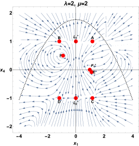
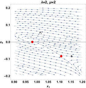
Figure 11: Phase-plot for system (60)-(61) for the fixed values $\mu=\lambda=2$, where the black-dashed parabola is $x_{4}=-\frac{-\mu^{4}+2x_{1}^{2}-4}{2\sqrt{2}\mu^{2}}$. Depicted on the left are the full dynamics of the system, while on the right is a close-up of the nearby points $F_{1}^{*}$ and $E$ to confirm the attracting behaviour of $F_{1}^{*}$.

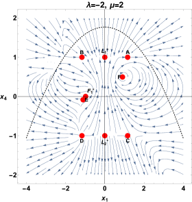
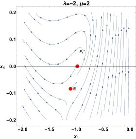
Figure 12: Phase-plot for system (60)-(61) for the fixed values $\mu=2,$ and $\lambda=-2$, where the black-dashed parabola is $x_{4}=-\frac{-\mu^{4}+2x_{1}^{2}-4}{2\sqrt{2}\mu^{2}}$. Depicted on the left are the full dynamics of the system, while on the right is a close-up of the nearby points $F_{1}^{*}$ and $E$ to be able to confirm the repelling behaviour of $F_{1}^{*}$.

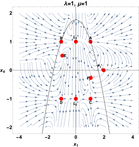
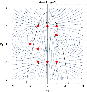
Figure 13: Phase-plot for system (60)-(61) for the fixed values $\mu=1$, and $\lambda=\pm 1$, where the black-dashed parabola is $x_{4}=-\frac{-\mu^{4}+2x_{1}^{2}-4}{2\sqrt{2}\mu^{2}}$. We observe that $F_{1}^{*}$ lies outside the parabola, but it still behaves as an attractor for $\lambda=1$ and a source for $\lambda=-1$.

Label	Attractor for $\lambda=\mu=2$	Attractor for $\lambda=-2,\mu=2$	Attractor for $\lambda=1,\mu=1$	Attractor for $\lambda=-1,\mu=1$
$F_{1}^{*}$	Yes, $\{-0.1363+0.1858i,-0.1363-0.1858i\}$	No, $\{0.1363+0.1858i,0.1363-0.1858i\}$	Yes, $\{-4.078,-0.2416\}$	No, $\{0.2416,4.078\}$
$L_{1}^{*}$	No, $\{2\sqrt{2},0\}$	Yes, $\{-2\sqrt{2},0\}$	No, $\{\sqrt{2},0\}$	Yes, $\{-\sqrt{2},0\}$
$L_{2}^{*}$	Yes, $\{-2\sqrt{2},0\}$	No, $\{2\sqrt{2},0\}$	Yes, $\{-\sqrt{2},0\}$	No, $\{\sqrt{2},0\}$
$A$	No, $\{3.142,0.3215\}$	No, $\{-2.515,0.3215\}$	No$,\{31.05,-503.6\}$	No, $\{28.22,-503.6\}$
$B$	No, $\{2.51454,-0.321462\}$	No$,\{-3.14231,-0.321462\}$	No, $\{-28.2179,503.621\}$	No, $\{-31.0464,503.621\}$
$C$	Yes, $\{-0.95474,-0.681949\}$	No, $\{4.70211,-0.681949\}$	No, $\{0.992799,-1.52955\}$	No, $\{3.82123,-1.52955\}$
$D$	No$,\{-4.70211,0.681949\}$	No$,\{0.95474,0.681949\}$	No, $\{-3.82123,1.52955\}$	No, $\par\{-0.992799,1.52955\}$
$E$	No, $\{-0.4658,0.1335\}$	No, $\{0.4658,-0.1335\}$	No, $\{0.7414+0.8029i,0.7414-0.8029i\}$	Yes, $\{-0.7414+0.8029i,-0.7414-0.8029i\}$
$F$	Yes, $\{-0.0119+0.9081i,-0.0119-0.9081i\}$	No, $\{0.0119+0.9081i,0.0119-0.9081i\}$	Yes, $\{-1.038,-0.2459\}$	No, $\{1.038,0.2459\}$

Table 5: Numerical stability analysis for the equilibrium points of system (60)-(61) for the fixed values of $\mu=1,2$ combined with $\lambda=\pm 1,\pm 2$. The stability for $L_{1}^{*}$ and $L_{2}^{*}$ refers to their behaviour along the axis line $x_{1}=0$.

IV Conclusions

In this section, we summarise the results of this research and present our final comments regarding our findings. This work focused on studying a five-dimensional Gauss-Bonnet with a scalar field coupled to the Gauss-Bonnet term via two different coupling functions. We derived the coupling term $GB_{5D}=8\dot{a}^{3}\left(f(\phi)+4a\dot{\phi}\frac{df}{d\phi}\right)$ after integrating by parts. Then we considered two specific models depending on the choice of the coupling function, say

1. $GB_{5D}=-8\alpha\dot{a}^{3}$, for $f(\phi)=-\alpha$,

2. $GB_{5D}=-8\alpha\dot{a}^{3}\left(\phi\dot{a}+4a\dot{\phi}\right)$, for $f(\phi)=-\alpha\phi$.

In both cases, the contribution to the field equations is not trivial. To begin, in section II, we presented a brief review of the tools from the theory of dynamical systems that were used in this research. In section III, we derived the field equations for the model using established techniques like integration by parts and the variation method of the point-like Lagrangian obtained from the gravitational action integral. We considered a quintessence scalar field and a phantom scalar field is left for future work.

In section III.1, we chose the constant coupling function to derive the field equations of the first model studied. We also wrote the Friedmann equation and defined the deceleration parameter. In the following section, that is section III.1.1, we defined $\chi-$normalised variables to derive the first four-dimensional dynamical system. Using Friedmann’s equation, we obtained constraints for the new variables that were used to reduce the dimension of the dynamical system. The analysis of the two-dimensional system (34)-(35) showed that this model has equilibrium points that describe super-collapsing scenarios like $P_{1,2,3,4}$ for which the deceleration parameter is $q=3$, as well as two scaling solutions $P_{5,6}$ for which $q=-1+\frac{3\lambda^{2}}{4}$. We formulated Theorem 2 to show that the model has late-time attractors. Furthermore, by restricting the parameter $\lambda$, only the scaling solution $P_{5}$ can be the late-time attractor. On the other hand, the other scaling solution $P_{6}$ is the early time attractor. In section III.1.2 we considered an alternative formulation of system (34)-(35) that takes advantage of the geometrical region described by the constraints on the $x_{i}$ variables. We defined the new system (40)-(41) for the new variables $\theta_{1}=\arctan\left(\frac{x_{2}}{x_{1}}\right)$, $\theta_{2}=\arctan\left(\frac{x_{4}}{x_{3}}\right)$ that represent the poloidal and toroidal directions of a torus defined by the parametrization $x=(R+r\cos(\theta_{1}-\pi))\cos(\theta_{2}-\pi),\quad y=(R+r\cos(\theta_{1}-\pi))\sin(\theta_{2}-\pi)$, and $z=r\sin(\theta_{1}-\pi)$. We showed that under this formulation, the two-dimensional dynamics of system (40)-(41) can be depicted on the surface of the previously mentioned torus. For the other choice of coupling function, in section III.2, we derived the field equations of the second model, wrote Friedmann’s equation and redefined the deceleration parameter. In section III.2.1, we used the same normalisation variable as before and derived the five-dimensional dynamical system for the model. Using the constraint, we reduced the dimension of the system to finally obtain the three-dimensional dynamical system (56)-(58). The analysis of the system showed once again that the model has equilibrium points that describe super-collapse that is $Q_{1,2,3,4}$ because $q=3$ and scaling solutions $Q_{5,6}$ since we verify that in this case $q=-1+\frac{3\lambda^{2}}{4}$. However, for this choice of coupling function, we also obtained three families of equilibrium points. In particular, the family $F_{1}$ describes a de Sitter solution because $q=1$. We formulated Theorem 3 to how all the possible attractors for the model but in particular, we can exclude the super-collapse point as late time attractors by setting $\lambda$ in one of the two intervals $-\frac{4}{\sqrt{3}}<\lambda<0$ or $0<\lambda<\frac{4}{\sqrt{3}}$ as stated in corollary 2. In section III.2.2 we considered a projection to a fixed value of $x_{5}=\mu$ since in the previous section, we obtained three equilibrium point families that depend on $x_{5}.$ To better observe the dynamics, we derived a new two-dimensional system (60)-(61) and studied the stability of its equilibrium points numerically for the values $\mu=1,2$ and different values of $\lambda.$ We verified the behaviour described in section III.2.1 in these two projections.

Comparing our results to those obtained in Millano:2023czt ; Millano:2023gkt where the authors studied a four-dimensional Gauss-Bonnet cosmology with a linear coupling function and a quintessence scalar field. The authors obtained stationary points with $\omega_{\phi}=-\frac{1}{3}$ corresponding to $q=0$ and points with $\omega_{\phi}=q=-1$, where $\omega_{\phi}$ is the effective equation of state parameter. They also considered a general exponential coupling function for which they obtained scaling solutions with $\omega_{\phi}=\frac{1}{3}(\lambda^{2}-3)$ corresponding to $q=\frac{1}{3}(\lambda^{2}-2)$. As stated before, scaling solutions are present in our model for both choices of the coupling function; we also have the Family $F_{1}$, which is a late-time de Sitter attractor. It is clear that the dimension of the background space plays an important role in the evolution of the cosmological parameters.

The models studied here showed that the scaling solutions can describe the early or the late time acceleration phase of the universe; this means that this model can be used to describe inflation and as a dark energy model.

References

• (1) E. J. Copeland, M. Sami and S. Tsujikawa, Int. J. Mod. Phys. D 15 (2006), 1753-1936 doi:10.1142/S021827180600942X [arXiv:hep-th/0603057 [hep-th]].
• (2) Y. F. Cai, E. N. Saridakis, M. R. Setare and J. Q. Xia, Phys. Rept. 493 (2010), 1-60 doi:10.1016/j.physrep.2010.04.001 [arXiv:0909.2776 [hep-th]].
• (3) E. N. Saridakis et al. [CANTATA], Springer, 2021, ISBN 978-3-030-83714-3, 978-3-030-83717-4, 978-3-030-83715-0 doi:10.1007/978-3-030-83715-0 [arXiv:2105.12582 [gr-qc]].
• (4) S. Capozziello and M. De Laurentis, Phys. Rept. 509 (2011), 167-321 doi:10.1016/j.physrep.2011.09.003 [arXiv:1108.6266 [gr-qc]].
• (5) S. Nojiri and S. D. Odintsov, Phys. Rept. 505 (2011), 59-144 doi:10.1016/j.physrep.2011.04.001 [arXiv:1011.0544 [gr-qc]].
• (6) A. R. Liddle and D. H. Lyth, Phys. Rept. 231 (1993), 1-105 doi:10.1016/0370-1573(93)90114-S [arXiv:astro-ph/9303019 [astro-ph]].
• (7) N. Aghanim et al. [Planck], Astron. Astrophys. 641 (2020), A6 [erratum: Astron. Astrophys. 652 (2021), C4] doi:10.1051/0004-6361/201833910 [arXiv:1807.06209 [astro-ph.CO]].
• (8) E. Abdalla, G. Franco Abellán, A. Aboubrahim, A. Agnello, O. Akarsu, Y. Akrami, G. Alestas, D. Aloni, L. Amendola and L. A. Anchordoqui, et al. JHEAp 34 (2022), 49-211 doi:10.1016/j.jheap.2022.04.002 [arXiv:2203.06142 [astro-ph.CO]].
• (9) S. Nojiri and S. D. Odintsov, Phys. Rev. D 74 (2006), 086005 doi:10.1103/PhysRevD.74.086005 [arXiv:hep-th/0608008 [hep-th]].
• (10) B. Famaey and S. McGaugh, Living Rev. Rel. 15 (2012), 10 doi:10.12942/lrr-2012-10 [arXiv:1112.3960 [astro-ph.CO]].
• (11) L. Sebastiani, S. Vagnozzi and R. Myrzakulov, Adv. High Energy Phys. 2017 (2017), 3156915 doi:10.1155/2017/3156915 [arXiv:1612.08661 [gr-qc]].
• (12) A. Addazi, J. Alvarez-Muniz, R. Alves Batista, G. Amelino-Camelia, V. Antonelli, M. Arzano, M. Asorey, J. L. Atteia, S. Bahamonde and F. Bajardi, et al. Prog. Part. Nucl. Phys. 125 (2022), 103948 doi:10.1016/j.ppnp.2022.103948 [arXiv:2111.05659 [hep-ph]].
• (13) A. De Felice and S. Tsujikawa, Living Rev. Rel. 13 (2010), 3 doi:10.12942/lrr-2010-3 [arXiv:1002.4928 [gr-qc]].
• (14) S. Nojiri and S. D. Odintsov, Phys. Lett. B 631 (2005), 1-6 doi:10.1016/j.physletb.2005.10.010 [arXiv:hep-th/0508049 [hep-th]].
• (15) A. De Felice and S. Tsujikawa, Phys. Lett. B 675 (2009), 1-8 doi:10.1016/j.physletb.2009.03.060 [arXiv:0810.5712 [hep-th]].
• (16) D. Lovelock, J. Math. Phys. 13, 874 (1972)
• (17) D. Lovelock, J. Math. Phys. 12, 498 (1971)
• (18) A. Mardones and J. Zanelli, Class. Quantum Grav. 8, 1545 (1991)
• (19) N. Deruelle and L. Farina-Busto, Phys. Rev. D 41 (1990), 3696 doi:10.1103/PhysRevD.41.3696
• (20) G. W. Horndeski, Int. J. Theor. Phys. 10 (1974), 363-384 doi:10.1007/BF01807638
• (21) A. De Felice and S. Tsujikawa, Phys. Rev. D 84 (2011), 124029 doi:10.1103/PhysRevD.84.124029 [arXiv:1008.4236 [hep-th]].
• (22) C. Deffayet, X. Gao, D. A. Steer and G. Zahariade, Phys. Rev. D 84 (2011), 064039 doi:10.1103/PhysRevD.84.064039 [arXiv:1103.3260 [hep-th]].
• (23) R. Aldrovandi and J. G. Pereira, Teleparallel Gravity: An Introduction, Springer, Dordrecht (2013).
• (24) J. W. Maluf, Annalen Phys. 525 (2013), 339-357 doi:10.1002/andp.201200272 [arXiv:1303.3897 [gr-qc]].
• (25) Y. F. Cai, S. Capozziello, M. De Laurentis and E. N. Saridakis, Rept. Prog. Phys. 79 (2016) no.10, 106901 doi:10.1088/0034-4885/79/10/106901 [arXiv:1511.07586 [gr-qc]].
• (26) R. Ferraro and F. Fiorini, Phys. Rev. D 75 (2007), 084031 doi:10.1103/PhysRevD.75.084031 [arXiv:gr-qc/0610067 [gr-qc]].
• (27) E. V. Linder, Phys. Rev. D 81 (2010), 127301 [erratum: Phys. Rev. D 82 (2010), 109902] doi:10.1103/PhysRevD.81.127301 [arXiv:1005.3039 [astro-ph.CO]].
• (28) G. Kofinas and E. N. Saridakis, Phys. Rev. D 90 (2014), 084044 doi:10.1103/PhysRevD.90.084044 [arXiv:1404.2249 [gr-qc]].
• (29) S. Bahamonde, C. G. Böhmer and M. Wright, Phys. Rev. D 92 (2015) no.10, 104042 doi:10.1103/PhysRevD.92.104042 [arXiv:1508.05120 [gr-qc]].
• (30) C. Q. Geng, C. C. Lee, E. N. Saridakis and Y. P. Wu, Phys. Lett. B 704 (2011), 384-387 doi:10.1016/j.physletb.2011.09.082 [arXiv:1109.1092 [hep-th]].
• (31) C. Q. Geng, C. C. Lee and E. N. Saridakis, JCAP 01 (2012), 002 doi:10.1088/1475-7516/2012/01/002 [arXiv:1110.0913 [astro-ph.CO]].
• (32) M. Gonzalez-Espinoza and G. Otalora, Eur. Phys. J. C 81 (2021) no.5, 480 doi:10.1140/epjc/s10052-021-09270-x [arXiv:2011.08377 [gr-qc]].
• (33) A. Paliathanasis, Universe 7 (2021) no.7, 244 doi:10.3390/universe7070244 [arXiv:2107.05880 [gr-qc]].
• (34) M. Gonzalez-Espinoza, R. Herrera, G. Otalora and J. Saavedra, Eur. Phys. J. C 81 (2021) no.8, 731 doi:10.1140/epjc/s10052-021-09542-6 [arXiv:2106.06145 [gr-qc]].
• (35) A. V. Toporensky and P. V. Tretyakov, Int. J. Geom. Meth. Mod. Phys. 19 (2022) no.10, 2250147 doi:10.1142/S021988782250147X [arXiv:2110.12332 [gr-qc]].
• (36) G. Kofinas, E. Papantonopoulos and E. N. Saridakis, Phys. Rev. D 91 (2015) no.10, 104034 doi:10.1103/PhysRevD.91.104034 [arXiv:1501.00365 [gr-qc]].
• (37) C. Q. Geng, C. C. Lee and H. H. Tseng, JCAP 11 (2012), 013 doi:10.1088/1475-7516/2012/11/013 [arXiv:1207.0579 [gr-qc]].
• (38) M. A. Skugoreva, E. N. Saridakis and A. V. Toporensky, Phys. Rev. D 91 (2015), 044023 doi:10.1103/PhysRevD.91.044023 [arXiv:1412.1502 [gr-qc]].
• (39) L. Jarv and A. Toporensky, Phys. Rev. D 93 (2016) no.2, 024051 doi:10.1103/PhysRevD.93.024051 [arXiv:1511.03933 [gr-qc]].
• (40) M. A. Skugoreva and A. V. Toporensky, Eur. Phys. J. C 76 (2016) no.6, 340 doi:10.1140/epjc/s10052-016-4190-x [arXiv:1605.01989 [gr-qc]].
• (41) M. Hohmann, L. Järv and U. Ualikhanova, Phys. Rev. D 97 (2018) no.10, 104011 doi:10.1103/PhysRevD.97.104011 [arXiv:1801.05786 [gr-qc]].
• (42) M. Hohmann, Phys. Rev. D 98 (2018) no.6, 064002 doi:10.1103/PhysRevD.98.064002 [arXiv:1801.06528 [gr-qc]].
• (43) M. Hohmann, Phys. Rev. D 98 (2018) no.6, 064004 doi:10.1103/PhysRevD.98.064004 [arXiv:1801.06531 [gr-qc]].
• (44) M. Hohmann and C. Pfeifer, Phys. Rev. D 98 (2018) no.6, 064003 doi:10.1103/PhysRevD.98.064003 [arXiv:1801.06536 [gr-qc]].
• (45) E. D. Emtsova and M. Hohmann, Phys. Rev. D 101 (2020) no.2, 024017 doi:10.1103/PhysRevD.101.024017 [arXiv:1909.09355 [gr-qc]].
• (46) S. Bahamonde, K. F. Dialektopoulos and J. Levi Said, Phys. Rev. D 100 (2019) no.6, 064018 doi:10.1103/PhysRevD.100.064018 [arXiv:1904.10791 [gr-qc]].
• (47) S. Bahamonde, K. F. Dialektopoulos, M. Hohmann and J. Levi Said, Class. Quant. Grav. 38 (2020) no.2, 025006 doi:10.1088/1361-6382/abc441 [arXiv:2003.11554 [gr-qc]].
• (48) S. Bahamonde, M. Caruana, K. F. Dialektopoulos, V. Gakis, M. Hohmann, J. Levi Said, E. N. Saridakis and J. Sultana, Phys. Rev. D 104 (2021) no.8, 084082 doi:10.1103/PhysRevD.104.084082 [arXiv:2105.13243 [gr-qc]].
• (49) R. C. Bernardo, J. L. Said, M. Caruana and S. Appleby, JCAP 10 (2021), 078 doi:10.1088/1475-7516/2021/10/078 [arXiv:2107.08762 [gr-qc]].
• (50) Y. Kucukakca, Eur. Phys. J. C 73 (2013) no.2, 2327 doi:10.1140/epjc/s10052-013-2327-8 [arXiv:1404.7315 [gr-qc]].
• (51) Y. Kucukakca, Eur. Phys. J. C 74 (2014) no.10, 3086 doi:10.1140/epjc/s10052-014-3086-x [arXiv:1407.1188 [gr-qc]].
• (52) G. Gecim and Y. Kucukakca, Int. J. Geom. Meth. Mod. Phys. 15 (2018) no.09, 1850151 doi:10.1142/S0219887818501517 [arXiv:1708.07430 [gr-qc]].
• (53) H. Mohseni Sadjadi, JCAP 01 (2017), 031 doi:10.1088/1475-7516/2017/01/031 [arXiv:1609.04292 [gr-qc]].
• (54) H. Mohseni Sadjadi, Phys. Rev. D 92 (2015) no.12, 123538 doi:10.1103/PhysRevD.92.123538 [arXiv:1510.02085 [gr-qc]].
• (55) R. Banerjee, S. Chakraborty and P. Mukherjee, Phys. Rev. D 98 (2018) no.8, 083506 doi:10.1103/PhysRevD.98.083506 [arXiv:1802.04150 [gr-qc]].
• (56) V. K. Sharma, B. K. Yadav and M. M. Verma, Eur. Phys. J. C 80 (2020) no.7, 619 doi:10.1140/epjc/s10052-020-8186-1 [arXiv:1912.12206 [gr-qc]].
• (57) V. K. Sharma, B. K. Yadav and M. M. Verma, Eur. Phys. J. C 81 (2021) no.2, 109 doi:10.1140/epjc/s10052-021-08908-0 [arXiv:2011.02878 [astro-ph.CO]].
• (58) P. S. Wesson, Int. J. Mod. Phys. D 24 (2014) no.01, 1530001 doi:10.1142/S0218271815300013 [arXiv:1412.6136 [gr-qc]].
• (59) Wesson, Paul S. Five-dimensional physics: classical and quantum consequences of Kaluza-Klein cosmology. World Scientific (2006)
• (60) Wesson, Paul S.; Ponce De Leon, J. Kaluza–Klein equations, Einstein’s equations, and an effective energy‐momentum tensor. J. Math. Phys. (1992), vol. 33, no 11, p. 3883-3887. https://doi.org/10.1063/1.529834.
• (61) O. Castillo-Felisola, C. Corral, S. del Pino and F. Ramírez, Phys. Rev. D 94 (2016) no.12, 124020 doi:10.1103/PhysRevD.94.124020 [arXiv:1609.09045 [gr-qc]].
• (62) L. Randall and R. Sundrum, Phys. Rev. Lett. 83 (1999), 4690-4693 doi:10.1103/PhysRevLett.83.4690 [arXiv:hep-th/9906064 [hep-th]].
• (63) N. Arkani-Hamed, S. Dimopoulos and G. R. Dvali, Phys. Rev. D 59 (1999), 086004 doi:10.1103/PhysRevD.59.086004 [arXiv:hep-ph/9807344 [hep-ph]].
• (64) S. G. Ghosh, M. Amir and S. D. Maharaj, Eur. Phys. J. C 77 (2017) no.8, 530 doi:10.1140/epjc/s10052-017-5099-8 [arXiv:1611.02936 [gr-qc]].
• (65) J. M. Armaleo, J. Osorio Morales and O. Santillan, Eur. Phys. J. C 78 (2018) no.2, 85 doi:10.1140/epjc/s10052-018-5558-x [arXiv:1711.09484 [gr-qc]].
• (66) S. Nojiri, S. D. Odintsov and M. Sasaki, Phys. Rev. D 71 (2005), 123509 doi:10.1103/PhysRevD.71.123509 [arXiv:hep-th/0504052 [hep-th]].
• (67) S. Nojiri, S. D. Odintsov and P. V. Tretyakov, Phys. Lett. B 651 (2007), 224-231 doi:10.1016/j.physletb.2007.06.029 [arXiv:0704.2520 [hep-th]].
• (68) G. Cognola, E. Elizalde, S. Nojiri, S. Odintsov and S. Zerbini, Phys. Rev. D 75 (2007), 086002 doi:10.1103/PhysRevD.75.086002 [arXiv:hep-th/0611198 [hep-th]].
• (69) S. Nojiri, S. D. Odintsov and M. Sami, Phys. Rev. D 74 (2006), 046004 doi:10.1103/PhysRevD.74.046004 [arXiv:hep-th/0605039 [hep-th]].
• (70) T. Padmanabhan and D. Kothawala, Phys. Rept. 531 (2013), 115-171 doi:10.1016/j.physrep.2013.05.007 [arXiv:1302.2151 [gr-qc]].
• (71) S. Chakraborty, T. Paul and S. SenGupta, Phys. Rev. D 98 (2018) no.8, 083539 doi:10.1103/PhysRevD.98.083539 [arXiv:1804.03004 [gr-qc]].
• (72) I. V. Fomin, Phys. Part. Nucl. 49 (2018) no.4, 525-529 doi:10.1134/S1063779618040226
• (73) P. Kanti, R. Gannouji and N. Dadhich, Phys. Rev. D 92 (2015) no.4, 041302 doi:10.1103/PhysRevD.92.041302 [arXiv:1503.01579 [hep-th]].
• (74) G. Hikmawan, J. Soda, A. Suroso and F. P. Zen, Phys. Rev. D 93 (2016) no.6, 068301 doi:10.1103/PhysRevD.93.068301 [arXiv:1512.00222 [hep-th]].
• (75) M. Motaharfar and H. R. Sepangi, Eur. Phys. J. C 76 (2016) no.11, 646 doi:10.1140/epjc/s10052-016-4474-1 [arXiv:1604.00453 [gr-qc]].
• (76) N. Rashidi and K. Nozari, Astrophys. J. 890, 58 doi:10.3847/1538-4357/ab6a10 [arXiv:2001.07012 [astro-ph.CO]].
• (77) A. D. Millano, G. Leon and A. Paliathanasis, Mathematics 11 (2023) no.6, 1408 doi:10.3390/math11061408 [arXiv:2302.09371 [gr-qc]].
• (78) A. D. Millano, G. Leon and A. Paliathanasis, Phys. Rev. D 108 (2023) no.2, 023519 doi:10.1103/PhysRevD.108.023519 [arXiv:2304.08659 [gr-qc]].
• (79) G. Leon, A. Millano and J. Latta, Eur. Phys. J. C 80 (2020) no.12, 1192 doi:10.1140/epjc/s10052-020-08731-z [arXiv:2010.03033 [gr-qc]].
• (80) A. D. Millano and G. Leon, Eur. Phys. J. C 84 (2024) no.1, 21 doi:10.1140/epjc/s10052-023-12366-1 [arXiv:2310.02741 [gr-qc]].
• (81) A. D. Millano, K. Dialektopoulos, N. Dimakis, A. Giacomini, H. Shababi, A. Halder and A. Paliathanasis, [arXiv:2403.06922 [gr-qc]].
• (82) G. Leon, A. Paliathanasis and A. D. Millano, Phys. Dark Univ. 44 (2024), 101459 doi:10.1016/j.dark.2024.101459 [arXiv:2307.01911 [gr-qc]].
• (83) L. Perko. Differential Equations and Dynamical Systems. Springer, Heidelberg (2013)
• (84) A. Coley. Dynamical Systems and Cosmology. Kluwer, Dordrecht (2003)
• (85) J. Tot, B. Yildirim, A. Coley and G. Leon, Phys. Dark Univ. 39 (2023), 101155 doi:10.1016/j.dark.2022.101155 [arXiv:2204.06538 [gr-qc]].
• (86) G. Leon, A. Coley, A. Paliathanasis, J. Tot and B. Yildirim, Phys. Dark Univ. 45 (2024), 101503 doi:10.1016/j.dark.2024.101503 [arXiv:2308.02470 [gr-qc]].