Inference in higher-order undirected graphical models and binary polynomial optimization

Abstract

We consider the problem of inference in higher-order undirected graphical models with binary labels. We formulate this problem as a binary polynomial optimization problem and propose several linear programming relaxations for it. We compare the strength of the proposed linear programming relaxations theoretically. Finally, we demonstrate the effectiveness of these relaxations by performing a computational study for two important applications, namely, image restoration and decoding error-correcting codes.

Key words: Graphical models; MAP estimator; Higher-order interactions; Binary polynomial optimization; Multilinear polytope; Linear programming relaxations.

1 Introduction

Graphical models are powerful probabilistic modeling tools for capturing complex relationships among large collections of random variables and have found ample applications in computer vision, natural language processing, signal processing, bioinformatics, and statistics [42]. In this framework, dependencies among random variables are represented by a graph. If this graph is a directed acyclic graph, the graphical model is often referred to as a Baysian Network, while if the graph is undirected, it is often referred to as an undirected graphical model or a Markov Random Field. In this paper, we focus on undirected graphical models (UGMs).

Undirected graphical models.

Let $G=(V,E)$ be an undirected graph, where $V,E$ denote node set and edge set of $G$, respectively. In order to define a graphical model, we associate with each node $v\in V$ a random variable $X_{v}$ taking values in some state space ${\mathcal{X}}_{v}$. The edge set $E$ represents dependencies between random variables; that is, for any three distinct nodes $u,v,w\in V$, $X_{u}$ is independent of $X_{v}$ given $X_{w}$, if every path from $u$ to $v$ in $G$ passes through $w$. The notation ${\mathbb{P}}(X_{v}=x_{v})$ corresponds to the probability of the event that the random variable $X_{v}$ takes the value $x_{v}\in{\mathcal{X}}_{v}$. Denote by ${\mathcal{C}}$ the set of maximal cliques in $G$; i.e., the set of cliques that are not properly contained in any other clique of $G$. Recall that a clique $C$ is a subset of $V$ such that $\{u,v\}\in E$ for all $u\neq v\in C$. For each $C\in{\mathcal{C}}$, let us define a nonnegative potential function $\phi_{C}(x_{C})$, where $x_{C}$ is the vector consisting of $x_{v}$, $v\in C$. In this paper, we assume ${\mathcal{X}}_{v}\in\{0,1\}$ for all $v\in V$, henceforth referred to as a binary UGM. It can be shown that the joint probability mass function for a binary UGM is given by:

$$p(x_{v},v\in V)={\mathbb{P}}(X_{v}=x_{v},v\in V)=\frac{1}{Z}\prod_{C\in{\mathcal{C}}}{\phi_{C}(x_{C})},$$ (1)

where $Z$ is a normalization constant given by $Z:=\sum_{x}{\prod_{C\in{\mathcal{C}}}\phi_{C}(x_{C})}$. The order of a UGM is defined as the size of a largest clique $C\in{\mathcal{C}}$ minus one. Due to their simplicity, first-order UGMs, also known as pair-wise models, are the most popular UGMs. However, to model more complex interactions among random variables it is essential to study higher-order UGMs.

Inference in binary UGMs.

Given some noisy observation $Y_{v}$, $v\in V$, we would like to recover the ground truth $X_{v}$, $v\in V$, whose probability mass function is described by a binary UGM defined by (1). By definition, the maximum a posteriori (MAP) estimator maximizes the probability of recovering the ground truth. In the following, we denote by ${\mathbb{P}}[X|Y]$ the probability that $X_{v}$, $v\in V$ is the ground truth given that $Y_{v}$, $v\in V$ is observed. Hence, we are interested in solving the following optimization problem:

$${\rm max}_{x\in\{0,1\}^{V}}\;{\mathbb{P}}[X|Y].$$ (2)

By Bayes’ theorem and monotonicity of the log function, we deduce that

$${\rm argmax}({\mathbb{P}}[X|Y])={\rm argmax}({\mathbb{P}}[Y|X]{\mathbb{P}}[X])={\rm argmax}(\log({\mathbb{P}}[Y|X]{\mathbb{P}}[X])).$$

Using (1), it follows that to solve Problem 2 we can equivalently solve:

$${\rm max}_{x\in\{0,1\}^{V}}\log({\mathbb{P}}[Y|X])+\sum_{C\in{\mathcal{C}}}{\log(\phi_{C}(x_{C}))}.$$ (3)

As we mentioned before, in this paper we consider binary UGMs. Suppose that $\phi_{C}(x_{C})>0$ for all $C\in{\mathcal{C}}$. It is well-known that any real-valued function in binary variables can be written as a binary polynomial function in the same variables. Given a clique $C$, denote by $P(C)$ the power set of $C$. Then Problem 3 can be equivalently written as:

$${\rm max}_{x\in\{0,1\}^{V}}\log({\mathbb{P}}[Y|X])+\sum_{C\in{\mathcal{C}}}{\sum_{e\in P(C)}c_{e}\prod_{v\in e}x_{v}}.$$ (4)

We should remark that if $\phi_{C}(x_{C})=0$ for some $x_{C}\in{\mathcal{X}}_{C}^{\prime}\subset\{0,1\}^{C}$, then one can proceed by adding the constraint $x_{C}\not\in{\mathcal{X}}^{\prime}_{C}$ to Problem 3. We use this technique in Section 4 to formulate the decoding problem. Now let us consider the first term in the objective function of Problem 4. To obtain an explicit description for ${\mathbb{P}}[Y|X]$, we have to make assumptions on the noise. In the following we introduce a simple noise model that we will also use in our numerical experiments. Given $p\in(0,\frac{1}{2}]$, the noisy observation $Y$ is constructed as follows: for each $v\in V$, $y_{v}$ is corrupted with probability $p$, i.e., $y_{v}=1-x_{v}$, and $y_{v}$ is not corrupted with probability $1-p$, i.e., $y_{v}=x_{v}$. We refer to this noise model as the bit-flipping noise. We then have

$${\mathbb{P}}\left[y_{v}\mid x_{v}\right]=\begin{cases}p^{x_{v}}(1-p)^{1-x_{v}}&\text{if $y_{v}=0$}\\ p^{1-x_{v}}(1-p)^{x_{v}}&\text{if $y_{v}=1$}.\end{cases}$$

Since the probability of corruption of the entries of $Y$ are independent, we have

$${\mathbb{P}}[Y\mid X]=\prod_{v\in V}{\mathbb{P}}\left[y_{v}\mid x_{v}\right]=\prod_{v\in V:y_{v}=0}{p^{x_{v}}(1-p)^{1-x_{v}}}\prod_{v\in V:y_{v}=1}{p^{1-x_{v}}(1-p)^{x_{v}}}.$$

We then deduce that under the bit-filliping noise, to solve Problem 4, it suffices to solve the following unconstrained binary polynomial optimization problem:

$${\rm max}_{x\in\{0,1\}^{V}}\log\Big{(}\frac{1-p}{p}\Big{)}\Big{(}\sum_{v\in V:y_{v}=1}{x_{v}}-\sum_{v\in V:y_{v}=0}{x_{v}}\Big{)}+\sum_{C\in{\mathcal{C}}}{\sum_{e\in P(C)}c_{e}\prod_{v\in e}x_{v}}.$$ (5)

Note that $\log\big{(}\frac{1-p}{p}\big{)}>0$, since by assumption $p\in(0,\frac{1}{2}]$. An optimal solution of Problem 5 is a MAP estimator under the bit-flipping noise and it requires parameter $p$ as an input. We would like to employ a formulation that does not have the knowledge of how the noisy observation was generated. That is, we propose to solve the following optimization problem:

$${\rm max}_{x\in\{0,1\}^{V}}\alpha\Big{(}\sum_{v\in V:y_{v}=1}{x_{v}}-\sum_{v\in V:y_{v}=0}{x_{v}}\Big{)}+\sum_{C\in{\mathcal{C}}}{\sum_{e\in P(C)}c_{e}\prod_{v\in e}x_{v}},$$ (6)

where $\alpha$ is a positive parameter that along with the remaining parameters $c_{e}$, $e\in P(C)$, $C\in{\mathcal{C}}$ should be learned from the data.

Literature review.

The literature on inference in UGMs is mostly focused on first-order UGMs; i.e., the case where $|C|=2$ for all $C\in{\mathcal{C}}$. For first-order binary UGMs, Problem 6 simplifies to an unconstrained binary quadratic optimization problem, which is NP-hard in general. The most popular methods to tackle this inference problem are belief propagation [41, 21], which is a message passing algorithm, and graph cut algorithms [32, 4, 5, 31]. Utilizing higher-order UGMs is essential for capturing more complex interactions among random variables. Yet, their study has been fairly limited due to the complexity of solving Problem 6 in its full generality. In fact, almost all existing studies considering higher-order UGMs tackle the inference problem by first reducing it to a binary quadratic optimization problem through the introduction of auxiliary variables and subsequently employing graph cut algorithms to solve the quadratic optimization problem [22, 38, 26, 27]. In [20], the authors consider the inference problem for a higher-order binary UGM arising from error-correcting decoding problem and propose a linear programming (LP) relaxation for this problem. In [19], the authors analyze the performance of the LP relaxation of [20] theoretically, hence establishing the effectiveness of the LP relaxation for decoding low-density-parity-check codes. In [8] the authors consider a third-order binary UGM for a simplified image restoration problem and propose an LP relaxation for this problem.

Our contributions.

In spite of its ample applications, existing results for inference in higher-order binary UGMs are rather scarce. In this paper, by building upon recent theoretical and algorithmic developments for binary polynomial optimization [10, 12, 11, 13, 16, 14], we present strong LP relaxations for Problem 6 in its full generality. We prove that the proposed LPs are stronger than the existing LPs for this class of problems and can be solved efficiently using off-the-shelf LP solvers. We consider two important applications of inference in higher-order binary UGMs; namely image restoration, a popular application in computer vision, and decoding error-correcting codes, a central problem in information theory. Via an extensive computational study, we show that a simple LP relaxation that we refer to as the “clique LP” is often sharp for image restoration problems. The decoding problem on the other hand turns out to be a difficult problem and while the proposed clique LP outperforms the only existing LP relaxation for this problem [19], the improvement is rather small.

Organization.

The remainder of this paper is structured as follows. In Section 2 we review existing LP relaxations for Problem 6 and propose new LP relaxations for it. In Section 3 we consider the image restoration problem while in Section 4 we consider the problem of decoding error-correcting codes.

2 Linear programming relaxations

With the objective of constructing LP relaxations for Problem 6, following a common practice in nonconvex optimization, we start by linearizing its objective function. For notational simplicity, henceforth we denote variables $x_{v}$, $v\in V$ by $z_{v}$, $v\in V$. Define $\bar{P}(C):=P(C)\setminus(C\cup\{\emptyset\})$ for all $C\in{\mathcal{C}}$. Define an auxiliary variable $z_{e}:=\prod_{v\in e}{z_{v}}$ for all $e\in\bar{P}(C)$ and for all $C\in{\mathcal{C}}$. Then an equivalent reformulation of Problem 6 in a lifted space of variables is given by:

$${\rm max}\quad \alpha\Big{(}\sum_{v\in V:y_{v}=1}{z_{v}}-\sum_{v\in V:y_{v}=0}{z_{v}}\Big{)}+\sum_{v\in V}{c_{v}z_{v}}+\sum_{C\in{\mathcal{C}}}{\sum_{e\in\bar{P}(C)}c_{e}z_{e}}$$ (B-UGM)

$${\rm s.t.}\quad z_{e}=\prod_{v\in e}{z_{v}},\;\forall e\in\bar{P}(C),\;\forall C\in{\mathcal{C}}$$

$$z_{v}\in\{0,1\},\;\forall v\in V.$$

Define the hypergraph ${\mathcal{G}}=(V,{\mathcal{E}})$ with the node set $V$ and the edge set ${\mathcal{E}}:=\cup_{C\in{\mathcal{C}}}{\bar{P}(C)}$. The rank of ${\mathcal{G}}$ is defined as the maximum cardinality of any edge in ${\mathcal{G}}$. Following the convention first introduced in [10], we define the multilinear set as:

$$S({\mathcal{G}})=\Big{\{}z\in\{0,1\}^{V\cup{\mathcal{E}}}:z_{e}=\prod_{v\in e}{z_{v}},\;\forall e\in\bar{P}(C),\;\forall C\in{\mathcal{C}}\Big{\}}.$$ (7)

We refer to the convex hull of $S({\mathcal{G}})$ as the multilinear polytope and denote it by $\text{MP}({\mathcal{G}})$. Henceforth, we refer to the hypergraph ${\mathcal{G}}$ associated with Problem B-UGM as the UGM hypergraph. To obtain an LP relaxation for Problem B-UGM, it suffices to construct a polyhedral relaxation for the multilinear set $S({\mathcal{G}})$. Notice that the rank of a UGM hypergraph equals the size of the largest clique $C$ in the corresponding UGM; this number in turn is always quite small in practice. This key property enables us to obtain strong and yet cheap relaxations for the multilinear polytope of a UGM hypergraph. In the remainder of this section, we briefly review existing LP relaxations for Problem B-UGM; subsequently, we propose new LP relaxations for it.

2.1 The standard linearization

The simplest and perhaps the oldest technique to convexify the multilinear set $S({\mathcal{G}})$ is to replace the feasible region defined by each product term $z_{e}=\prod_{v\in e}z_{v}$ over the set of binary points with its convex hull. We then obtain our first polyhedral relaxation of $S({\mathcal{G}})$:

$$\text{MP}^{\text{LP}}({\mathcal{G}})=\Big{\{}z:\; z_{v}\leq 1,\;\forall v\in V,z_{e}\geq 0,\;z_{e}\geq\sum_{v\in e}{z_{v}}-|e|+1,\;\forall e\in\bar{P}(C),\forall C\in{\mathcal{C}},$$

$$z_{e}\leq z_{v},\forall v\in e,\;e\in\bar{P}(C),\forall C\in{\mathcal{C}}\Big{\}}.$$ (8)

The above relaxation has been used extensively in the literature and is often referred to as the standard linearization of the multilinear set (see for example [25, 7]). We then define our first LP relaxation which we refer to as the standard LP:

$$\max\quad \alpha\Big{(}\sum_{v\in V:y_{v}=1}{z_{v}}-\sum_{v\in V:y_{v}=0}{z_{v}}\Big{)}+\sum_{v\in V}{c_{v}z_{v}}+\sum_{C\in{\mathcal{C}}}{\sum_{e\in\bar{P}(C)}c_{e}z_{e}}$$ (stdLP)

$${\rm s.t.}\quad z\in\text{MP}^{\text{LP}}({\mathcal{G}}).$$

In [11, 6], the authors prove that $\text{MP}^{\text{LP}}({\mathcal{G}})=\text{MP}({\mathcal{G}})$ if and only if ${\mathcal{G}}$ is a Berge-acyclic hypergraph; i.e., the most restrictive type of hypergraph acyclicity [18]. However, a UGM hypergraph is not Berge-acyclic and indeed our numerical experiments indicate that Problem stdLP leads to very weak upper bounds for Problem B-UGM.

2.2 The flower relaxation

In [11], the authors introduce flower inequalities, a family of valid inequalities for the multilinear polytope, which strengthens the standard linearization. Flower inequalities were later generalized in [30] and in the following we use this more general definition. Let $e_{0},e_{k}$, $k\in T$, $T\neq\emptyset$ be edges of ${\mathcal{G}}$ such that

$$\Big{|}(e_{0}\cap e_{k})\setminus\bigcup_{j\in T\setminus\{k\}}{(e_{0}\cap e_{j})}\Big{|}\geq 2,\quad\forall k\in T.$$ (9)

Then the flower inequality centered at $e_{0}$ with neighbors $e_{k}$, $k\in T$, is given by:

$$\sum_{v\in e_{0}\setminus\cup_{k\in T}{e_{k}}}{z_{v}}+\sum_{k\in T}{z_{e_{k}}}-z_{e_{0}}\leq|e_{0}\setminus\cup_{k\in T}{e_{k}}|+|T|-1.$$ (10)

If $|T|=1$, flower inequalities simplify to two-link inequalities introduced in [8]. We define the flower relaxation $\text{MP}^{F}({\mathcal{G}})$ as the polytope obtained by adding all flower inequalities centered at each edge of ${\mathcal{G}}$ to $\text{MP}^{\text{LP}}({\mathcal{G}})$. In [16], the authors prove that while the separation problem over the flower relaxation is ${\mathcal{N}P}$-hard for general hypergraphs, it can be solved in polynomial time for hypergraphs with fixed rank. As we discussed before, in case of a UGM hypergraph, it is reasonable to assume that $r$ is fixed. In fact, as we show next, for a UGM hypergraph, it suffices to include only a small number of flower inequalities in the flower relaxation.

Lemma 1.

Let ${\mathcal{G}}=(V,{\mathcal{E}})$ with ${\mathcal{E}}=\cup_{C\in{\mathcal{C}}}{\bar{P}(C)}$ be a UGM hypergraph and consider the flower relaxation $\text{MP}^{F}({\mathcal{G}})$ of $S({\mathcal{G}})$. Denote by $\text{MP}^{F^{\prime}}({\mathcal{G}})$ the polytope obtained by adding all flower inequalities (10) satisfying

$$\gamma(e_{0},e_{k},k\in T):=\bigcup_{k\in T}{e_{k}}\cup e_{0}\subseteq C,\quad{\rm for\;some}\;C\in{\mathcal{C}},$$ (11)

to the standard linearization. Then $\text{MP}^{F}({\mathcal{G}})=\text{MP}^{F^{\prime}}({\mathcal{G}})$.

Proof.

Let $e_{0},e_{k}$, $k\in T$ be edges of ${\mathcal{G}}$ satisfying condition (9) but not satisfying condition (11). Then the following flower inequality is present in $\text{MP}^{F}({\mathcal{G}})$:

$$\sum_{v\in e_{0}\setminus\cup_{k\in T}{e_{k}}}{z_{v}}+\sum_{k\in T}{z_{e_{k}}}-z_{e_{0}}\leq|e_{0}\setminus\cup_{k\in T}{e_{k}}|+|T|-1.$$ (12)

First consider the case where $e_{j}\supset e_{0}$ for some $j\in T$; then by (9) we must have $|T|=1$, implying that $\gamma(e_{0},e_{j})=e_{j}$ and hence condition (11) holds. Henceforth, suppose that $e_{k}\not\supset e_{0}$ for all $k\in T$. Notice that if $e_{k}\subset e_{0}$ for all $k\in T$, then we have $\gamma(e_{0},e_{k},k\in T)=e_{0}$ and condition (11) is trivially satisfied. Denote by $T^{\prime}$ the nonempty set containing all $k\in T$ satisfying $e_{k}\setminus e_{0}\neq\emptyset$. Define $\tilde{e}_{k}=e_{k}\cap e_{0}$ for all $k\in T^{\prime}$. By definition of a UGM hypergraph and condition (9), we have $\tilde{e}_{k}\in{\mathcal{E}}$ for all $k\in T^{\prime}$. Hence the following flower inequalities are also present in $\text{MP}^{F}({\mathcal{G}})$:

$$\sum_{v\in e_{0}\setminus\cup_{k\in T}{e_{k}}} {z_{v}}+\sum_{k\in T\setminus T^{\prime}}{z_{e_{k}}}+\sum_{k\in T^{\prime}}{z_{\tilde{e}_{k}}}-z_{e_{0}}\leq|e_{0}\setminus\cup_{k\in T}{e_{k}}|+|T|-1$$ (13)

$$z_{e_{k}}-z_{\tilde{e}_{k}}\leq 0,\quad\forall k\in T^{\prime},$$ (14)

where we used $e_{0}\setminus\cup_{k\in T}{e_{k}}=e_{0}\setminus(\cup_{k\in T\setminus T^{\prime}}{e_{k}}\cup\cup_{k\in T^{\prime}}{\tilde{e}_{k}})$. First, it is simple to verify that condition (11) is satisfied for inequalities (13) and (14). Second, summing up inequalities (13) and (14), we obtain inequality (12), implying its redundancy, and this completes the proof. ∎

We then define our next LP relaxation, which we refer to as the flower LP:

$$\max\quad \alpha\Big{(}\sum_{v\in V:y_{v}=1}{z_{v}}-\sum_{v\in V:y_{v}=0}{z_{v}}\Big{)}+\sum_{v\in V}{c_{v}z_{v}}+\sum_{C\in{\mathcal{C}}}{\sum_{e\in\bar{P}(C)}c_{e}z_{e}}$$ (flLP)

$${\rm s.t.}\quad z\in\text{MP}^{F}({\mathcal{G}}).$$

In [11], the authors prove that $\text{MP}^{F}({\mathcal{G}})=\text{MP}({\mathcal{G}})$ if and only if ${\mathcal{G}}$ is a $\gamma$-acyclic hypergraph. Note that $\gamma$-acyclic hypergraphs represent a significant generalization of Berge-acyclic hypergraphs [18]. While a UGM hypergraph is not $\gamma$-acyclic in general, as we show in our numerical experiments, the flower LP is significantly stronger than the standard LP.

2.3 The running intersection relaxation

In [13], the authors introduce running intersection inequalities, a family of valid inequalities for the multilinear polytope, which strengthens the flower relaxation (see [16] for a detailed computational study). Running intersection inequalities were later generalized in [14] and in the following we use this more general definition. To define these inequalities, we first introduce the notion of running intersection property [3]. A set $F$ of subsets of a finite set $V$ has the running intersection property if there exists an ordering $p_{1},p_{2},\ldots,p_{m}$ of the sets in $F$ such that

for each $$k=2,\dots,m j<k p_{k}\cap\Big{(}\bigcup_{i<k}{p_{i}}\Big{)}\subseteq p_{j}$$, there exists such that . (15)

We refer to an ordering $p_{1},p_{2},\ldots,p_{m}$ satisfying (15) as a running intersection ordering of $F$. Each running intersection ordering $p_{1},p_{2},\ldots,p_{m}$ of $F$ induces a collection of sets

$$N(p_{1}):=\emptyset,\qquad N(p_{k}):=p_{k}\cap\Big{(}\bigcup_{i<k}{p_{i}}\Big{)}\text{ for }k=2,\dots,m.$$ (16)

We are now ready to define running intersection inequalities. Let $e_{0}$, $e_{k}$, $k\in T$, be edges of ${\mathcal{G}}$ such that

• $|e_{0}\cap e_{k}|\geq 2$ for all $k\in T$,

• $e_{0}\cap e_{k}\not\subseteq e_{0}\cap e_{k^{\prime}}$ for any $k\neq k^{\prime}\in T$,

• the set $\tilde{E}:=\{e_{0}\cap e_{k}:k\in T\}$ has the running intersection property.

Consider a running intersection ordering of $\tilde{E}$ with the sets $N(e_{0}\cap e_{k})$, for all $k\in T$, as defined in (16). For each $k\in T$, let $w_{k}\subseteq N(e_{0}\cap e_{k})$ such that $w_{k}\in\{\emptyset\}\cup V\cup{\mathcal{E}}$. We define a running intersection inequality centered at $e_{0}$ with neighbors $e_{k}$, $k\in T$ as:

$$-\sum_{k\in T}z_{w_{k}}+\sum_{v\in e_{0}\setminus\bigcup_{k\in T}e_{k}}z_{v}+\sum_{k\in T}{z_{e_{k}}}-z_{e_{0}}\leq\omega-1,$$ (17)

where we define $z_{\emptyset}=0$, and

$$\omega=\Big{|}e_{0}\setminus\bigcup_{k\in T}e_{k}\Big{|}+\Big{|}\Big{\{}k\in T:N(e_{0}\cap e_{k})=\emptyset\Big{\}}\Big{|}.$$

Notice that by letting $w_{k}=\emptyset$ for all $k\in T$, the running intersection inequality (17) simplifies to the flower inequality (10). Consider $e_{0},e_{k}$, $k\in T$ such that $\tilde{E}$ has the running intersection property and $N(e_{0}\cap e_{k})\neq\emptyset$ for some $k\in T$. Then any running intersection inequality centered at $e_{0}$ with neighbours $e_{k}$, $k\in T$ satisfying $w_{k}\neq\emptyset$ for some $k\in T$ together with $z_{w_{k}}\leq 1$ imply the flower inequality centered at $e_{0}$ with neighbours $e_{k}$, $k\in T$. However, in general flower inequalities are not implied by running intersection inequalities, since for flower inequalities we do not require the set $\tilde{E}$ to have the running intersection property.

We then define the running intersection relaxation of $S({\mathcal{G}})$, denoted by $\text{MP}^{\rm RI}({\mathcal{G}})$, as the polytope obtained by adding to the flower relaxation, all running intersection inequalities of $S({\mathcal{G}})$. As in the case of flower inequalities, for a UGM hypergraph, we can establish the redundancy of a large number of running intersection inequalities:

Lemma 2.

Let ${\mathcal{G}}=(V,{\mathcal{E}})$ with ${\mathcal{E}}=\cup_{C\in{\mathcal{C}}}{\bar{P}(C)}$ be a UGM hypergraph and consider the running intersection relaxation $\text{MP}^{\rm RI}({\mathcal{G}})$ of $S({\mathcal{G}})$. Denote by $\text{MP}^{\rm RI^{\prime}}({\mathcal{G}})$ the polytope obtained by adding all running intersection inequalities (10) satisfying condition (11) to the flower relaxation. Then $\text{MP}^{\rm RI}({\mathcal{G}})=\text{MP}^{\rm RI^{\prime}}({\mathcal{G}})$.

Proof.

The proof follows from a similar line of arguments to those in the proof of Lemma 1. ∎

We then define our next LP relaxation, which we refer to as the running LP:

$$\max\quad \alpha\Big{(}\sum_{v\in V:y_{v}=1}{z_{v}}-\sum_{v\in V:y_{v}=0}{z_{v}}\Big{)}+\sum_{v\in V}{c_{v}z_{v}}+\sum_{C\in{\mathcal{C}}}{\sum_{e\in\bar{P}(C)}c_{e}z_{e}}$$ (runLP)

$${\rm s.t.}\quad z\in\text{MP}^{\rm RI}({\mathcal{G}}).$$

In [16], the authors prove that for hypergraphs with fixed rank, the separation problem over running intersection inequalities can be solve in polynomial time. Our computational results indicate that the running LP is significantly stronger than the flower LP. However, the added strength often comes at the cost of a rather significant increase in CPU time.

2.4 The clique relaxation

A hypergraph $\bar{G}$ with node set $\bar{V}$ is a complete hypergraph, if its edge set consists of all subsets of $\bar{V}$ of cardinality at least two. It then follows that a UGM hypergraph ${\mathcal{G}}=(V,{\mathcal{E}})$ with ${\mathcal{E}}=\cup_{C\in{\mathcal{C}}}{\bar{P}(C)}$ can be written as a union of complete hypergraphs ${\mathcal{G}}=\cup_{C\in{\mathcal{C}}}{{\mathcal{G}}_{C}}$, where ${\mathcal{G}}_{C}$ denotes a complete hypergraph with node set $C$. We then define the clique relaxation of the multilinear set, denoted by $\text{MP}^{\rm cl}({\mathcal{G}})$, as the polytope obtained by intersecting all multilinear polytopes of complete hypergraphs; i.e., $\text{MP}({\mathcal{G}}_{C})$ for all $C\in{\mathcal{C}}$. An explicit description for the multilinear polytope of a complete hypergraph can be obtained using Reformulation Linearization Technique (RLT) [39]. For completeness, we present this description next.

Proposition 1.

(Theorem 2 in [39]) Let ${\mathcal{G}}_{C}$ be a complete hypergraph with node set $C$. Then the multilinear polytope $\text{MP}({\mathcal{G}}_{C})$ is given by

$$\psi_{U}(z_{C})\geq 0\quad\forall U\subseteq C,$$ (18)

where

$$\psi_{U}(z_{C}):=\sum_{\begin{subarray}{c}W\subseteq C\cap U:\\ |W|\;{\rm even}\end{subarray}}{z_{(C\setminus U)\cup W}}-\sum_{\begin{subarray}{c}W\subseteq C\cap U:\\ |W|\;{\rm odd}\end{subarray}}{z_{(C\setminus U)\cup W}},$$ (19)

and we define $z_{\emptyset}:=1$.

By Proposition 1, the clique relaxation $\text{MP}^{\rm cl}({\mathcal{G}})$ consist of $\sum_{C\in{\mathcal{C}}}{2^{|C|}}$ inequalities. Hence, this relaxation is computationally tractable only if the rank of the UGM hypergraph is small; a property that is present in all relevant applications. We now define our next LP relaxation which we refer to as the clique LP:

$$\max\quad \alpha\Big{(}\sum_{v\in V:y_{v}=1}{z_{v}}-\sum_{v\in V:y_{v}=0}{z_{v}}\Big{)}+\sum_{v\in V}{c_{v}z_{v}}+\sum_{C\in{\mathcal{C}}}{\sum_{e\in\bar{P}(C)}c_{e}z_{e}}$$ (cliqueLP)

$${\rm s.t.}\quad z\in\text{MP}^{\rm cl}({\mathcal{G}}).$$

In Sections 3 and 4 we show that the clique LP returns a binary solution in many cases of practical interest. We next present a theoretical justification of this fact. That is, we show that all inequalities defining facets of the clique relaxation $\text{MP}^{\rm cl}({\mathcal{G}})$ are facet-defining for the multilinear polytope $\text{MP}({\mathcal{G}})$ as well. To this end, we make use of a zero-lifting operation for the multilinear polytope that was introduced in [10]. Let ${\mathcal{G}}=(V,{\mathcal{E}})$ be a hypergraph. Then the hypergraph ${\mathcal{G}}^{\prime}=(V^{\prime},{\mathcal{E}}^{\prime})$ is a partial hypergraph of ${\mathcal{G}}$ if $V^{\prime}\subseteq V$ and ${\mathcal{E}}^{\prime}\subseteq{\mathcal{E}}$. The following lemma [10], provides a sufficient condition under which a facet-defining inequality for $\text{MP}({\mathcal{G}}^{\prime})$ is also facet-defining for $\text{MP}({\mathcal{G}})$.

Lemma 3.

(Corollary 4 in [10]) Let the complete hypergraph ${\mathcal{G}}^{\prime}=(V^{\prime},{\mathcal{E}}^{\prime})$ be a partial hypergraph of ${\mathcal{G}}=(V,{\mathcal{E}})$. Then all facet-defining inequalities for $\text{MP}({\mathcal{G}}^{\prime})$ are facet-defining for $\text{MP}({\mathcal{G}})$ if and only if there exists no edge $e\in{\mathcal{E}}$ such that $e\supset V^{\prime}$.

The following result establishes the strength of the clique relaxation:

Proposition 2.

Let ${\mathcal{G}}=\cup_{C\in{\mathcal{C}}}{{\mathcal{G}}_{C}}$ be a UGM hypergraph where ${\mathcal{C}}$ denotes the set of maximal clique of the binary UGM. Then for any $C\in{\mathcal{C}}$, all facet-defining inequalities of $\text{MP}({\mathcal{G}}_{C})$ are facet defining for $\text{MP}({\mathcal{G}})$ as well.

Proof.

Since $C\in{\mathcal{C}}$ is a maximal clique of the UGM, by definition, there exists no edge $e\in{\mathcal{E}}$ that strictly contains $C$. Hence assumptions of Lemma 3 are satisfied and the result follows. ∎

By construction, for a general UGM hypergraph ${\mathcal{G}}$ we have $\text{MP}^{\text{LP}}({\mathcal{G}})\subset\text{MP}^{F}({\mathcal{G}})\subset\text{MP}^{\rm RI}({\mathcal{G}})$. The next result indicates that the clique relaxation $\text{MP}^{\rm cl}({\mathcal{G}})$ is the strongest relaxation of $\text{MP}({\mathcal{G}})$ introduced so far.

Proposition 3.

Let ${\mathcal{G}}=\cup_{C\in{\mathcal{C}}}{{\mathcal{G}}_{C}}$ be a UGM hypergraph of rank $r\geq 3$, where ${\mathcal{C}}$ denotes the set of maximal clique of the binary UGM. Then $\text{MP}^{\rm cl}({\mathcal{G}})\subsetneq\text{MP}^{\rm RI}({\mathcal{G}})$.

Proof.

Consider any inequality in the description of $\text{MP}^{\rm RI}({\mathcal{G}})$. Then from the definition of the standard linearization together with Lemmas 1 and 2, it follows that this inequality is also a valid inequality for the multilinear polytope $\text{MP}({\mathcal{G}}_{C})$ for some $C\in{\mathcal{C}}$, and hence is implied by inequalities defining $\text{MP}^{\rm cl}({\mathcal{G}})$. Moreover, $\text{MP}^{\rm cl}({\mathcal{G}})$ is strictly contained in $\text{MP}^{\rm RI}({\mathcal{G}})$ since for example its facet-defining inequality (18) with $U=C$ is given by

$$\sum_{\begin{subarray}{c}W\subseteq C:\\ |W|\;{\rm even}\end{subarray}}{z_{W}}-\sum_{\begin{subarray}{c}W\subseteq C:\\ |W|\;{\rm odd}\end{subarray}}{z_{W}}\geq 0,$$

which is clearly not present in $\text{MP}^{\rm RI}({\mathcal{G}})$, if $|C|\geq 3$. ∎

Next we provide a necessary and sufficient condition under which the clique relaxation coincides with the multilinear polytope. To this end we make use of two tools which we present first. First, we outline a sufficient condition for decomposability of multilinear sets [12]. Let ${\mathcal{G}}=(V,{\mathcal{E}})$ be a hypergraph and let ${\mathcal{G}}^{\prime}=(V^{\prime},{\mathcal{E}}^{\prime})$ be a partial hypergraph of ${\mathcal{G}}$. Then ${\mathcal{G}}^{\prime}$ is a section hypergraph of ${\mathcal{G}}$ induced by $V^{\prime}$, if ${\mathcal{E}}^{\prime}=\{e\in{\mathcal{E}}:e\subseteq V^{\prime}\}$. In the following, given hypergraphs ${\mathcal{G}}_{1}=(V_{1},{\mathcal{E}}_{1})$ and ${\mathcal{G}}_{2}=(V_{2},{\mathcal{E}}_{2})$, we denote by ${\mathcal{G}}_{1}\cap{\mathcal{G}}_{2}$ the hypergraph $(V_{1}\cap V_{2},{\mathcal{E}}_{1}\cap{\mathcal{E}}_{2})$, and we denote by ${\mathcal{G}}_{1}\cup{\mathcal{G}}_{2}$, the hypergraph $(V_{1}\cup V_{2},{\mathcal{E}}_{1}\cup{\mathcal{E}}_{2})$. Finally, we say that the multilinear set $S({\mathcal{G}})$ is decomposable into $S({\mathcal{G}}_{1})$ and $S({\mathcal{G}}_{2})$ if the system comprised of the description of $\text{MP}({\mathcal{G}}_{1})$ and the description of $\text{MP}({\mathcal{G}}_{2})$, is the description of $\text{MP}({\mathcal{G}})$.

Theorem 1 (Theorem 1 in [12]).

Let ${\mathcal{G}}$ be a hypergraph, and let ${\mathcal{G}}_{1},{\mathcal{G}}_{2}$ be section hypergraphs of ${\mathcal{G}}$ such that ${\mathcal{G}}_{1}\cup{\mathcal{G}}_{2}={\mathcal{G}}$ and ${\mathcal{G}}_{1}\cap{\mathcal{G}}_{2}$ is a complete hypergraph. Then the set $S({\mathcal{G}})$ is decomposable into $S({\mathcal{G}}_{1})$ and $S({\mathcal{G}}_{2})$.

Consider a hypergraph ${\mathcal{G}}=(V,{\mathcal{E}})$ and let $V^{\prime}$ be a subset of $V$. We define the subhypergraph of ${\mathcal{G}}$ induced by $V^{\prime}$ as the hypergraph ${\mathcal{G}}_{V^{\prime}}$ with node set $V^{\prime}$ and with edge set $\{e\cap V^{\prime}:e\in{\mathcal{E}},|e\cap V^{\prime}|\geq 2\}$. For every edge $e$ of ${\mathcal{G}}_{V^{\prime}}$, there may exist several edges $e^{\prime}$ of ${\mathcal{G}}$ satisfying $e=e^{\prime}\cap V$; we denote by $e^{\prime}(e)$ one such arbitrary edge of ${\mathcal{G}}$. For ease of notation, we identify an edge $e$ of ${\mathcal{G}}_{V^{\prime}}$ with an edge $e^{\prime}(e)$ of ${\mathcal{G}}$. Define

$$L_{\bar{V}}:=\{z\in{\mathbb{R}}^{V+{\mathcal{E}}}:z_{v}=1\ \forall v\in V\setminus\bar{V}\}.$$ (20)

Denote by ${\rm proj}_{{\mathcal{G}}_{V^{\prime}}}(\text{MP}({\mathcal{G}})\cap L_{V^{\prime}})$ the set obtained from $\text{MP}({\mathcal{G}})\cap L_{V^{\prime}}$ by projecting out all variables $z_{v}$, for all $v\in V\setminus V^{\prime}$, and $z_{f}$, for all $f\in{\mathcal{E}}\setminus\{e^{\prime}(e):e\in{\mathcal{E}}_{V^{\prime}}\}$, where ${\mathcal{E}}_{V^{\prime}}$ denotes the edge set of ${\mathcal{G}}_{V^{\prime}}$. In [11], the authors prove the following equivalence:

Lemma 4 (Lemma 6 in [11]).

Let ${\mathcal{G}}=(V,{\mathcal{E}})$ be a hypergraph and let $L_{V^{\prime}}$ be a set defined by (20) for some $V^{\prime}\subseteq V$. Then $\text{MP}({\mathcal{G}}_{V^{\prime}})={\rm proj}_{{\mathcal{G}}_{V^{\prime}}}(\text{MP}({\mathcal{G}})\cap L_{V^{\prime}})$.

The next proposition characterizes UGM hypergraphs for which $\text{MP}^{\rm cl}({\mathcal{G}})=\text{MP}({\mathcal{G}})$.

Proposition 4.

Let ${\mathcal{G}}=\cup_{C\in{\mathcal{C}}}{{\mathcal{G}}_{C}}$ be a UGM hypergraph where ${\mathcal{C}}$ denotes the set of maximal clique of the binary UGM and ${\mathcal{G}}_{C}$ is a complete hypergraph with node set $C$. Then $\text{MP}^{\rm cl}({\mathcal{G}})=\text{MP}({\mathcal{G}})$ if and only if ${\mathcal{C}}$ has the running intersection property.

Proof.

Denote by $C_{1},C_{2},\cdots,C_{m}$ a running intersection ordering of ${\mathcal{C}}$. Let ${\mathcal{G}}_{i}$ denote the complete hypergraph with node set $C_{i}$ for all $i\in\{1,\cdots,m\}$. Define ${\mathcal{G}}^{\prime}_{m}=\cup_{i=1}^{m-1}{{\mathcal{G}}_{i}}$. Then by definition of the running intersection ordering, ${\mathcal{G}}_{m}\cap{\mathcal{G}}^{\prime}_{m}$ is a section hypergraph of ${\mathcal{G}}_{i}$ for some $i\in\{1,\cdots,m-1\}$ and hence is a complete hypergraph. Hence, by Theorem 1 the set $S({\mathcal{G}})$ is decomposable into $S({\mathcal{G}}_{m})$ and $S({\mathcal{G}}^{\prime}_{m})$. By a recursive application of this argument $m$ times we conclude that $S({\mathcal{G}})$ is decomposable into multilinear sets $S({\mathcal{G}}_{i})$, $i\in\{1,\cdots,m\}$, implying $\text{MP}^{\rm cl}({\mathcal{G}})=\text{MP}({\mathcal{G}})$.

Now suppose that the set ${\mathcal{C}}$ does not have the running intersection property. This in turn implies that the edge set of ${\mathcal{G}}$ does not have the running intersection property either. Denote by $V$ the node set of ${\mathcal{G}}$. By Lemma 4 to prove $\text{MP}({\mathcal{G}})\subset\text{MP}^{\rm cl}({\mathcal{G}})$, it suffices to show that $\text{MP}({\mathcal{G}}_{V^{\prime}})\subset\text{MP}^{\rm cl}({\mathcal{G}}_{V^{\prime}})$ for some $V^{\prime}\subseteq V$. Let $V^{\prime}\subseteq V$ be such that the edge set ${\mathcal{E}}^{\prime}$ of ${\mathcal{G}}_{V^{\prime}}$ does not have the running intersection property, while the edge set of ${\mathcal{G}}_{V^{\prime\prime}}$ for any $V^{\prime\prime}\subset V^{\prime}$ has the running intersection property. First, note that ${\mathcal{G}}_{V^{\prime}}$ must contain $\beta$-cycles as otherwise ${\mathcal{E}}^{\prime}$ has the running intersection property. Second ${\mathcal{G}}_{V^{\prime}}$ does not contain an edge $e=V^{\prime}$ as otherwise ${\mathcal{E}}^{\prime}$ again has the running intersection property. It then follows that ${\mathcal{G}}_{V^{\prime}}$ is a graph that is a chordless cycle as otherwise there exists $V^{\prime\prime}\subset V^{\prime}$ such that ${\mathcal{G}}_{V^{\prime\prime}}$ a chordless cycle implying that its edge set does not have the running intersection property. The inclusion $\text{MP}({\mathcal{G}}_{V^{\prime}})\subset\text{MP}^{\rm cl}({\mathcal{G}}_{V^{\prime}})$ then follows since odd-cylce inequalities are facet-defining for $\text{MP}({\mathcal{G}}_{V^{\prime}})$ [36] and are not implied by $\text{MP}^{\rm cl}({\mathcal{G}}_{V^{\prime}})$, which only contains McCormick type inequalities. ∎

2.5 The multi-clique relaxation

By Proposition 3, the clique relaxation is the strongest LP relaxation introduced so far. Yet by Proposition 4, this LP is guaranteed to solve the original problem if the set of cliques ${\mathcal{C}}$ has the running intersection property; a property that is often not present in applications. In this section we propose stronger LP relaxations for Problem B-UGM by constructing the multilinear polytope of a UGM hypergraph containing multiple cliques that do not have the running intersection property. More precisely, we consider a special structure, that we refer to as the cycle of cliques, and obtain the multilinear polytope using disjunctive programming [2]. This structure appears in applications such as image restoration and decoding problems.

Consider the set of maximal cliques ${\mathcal{C}}:=\{C_{1},C_{2},\ldots,C_{m}\}$, where $m\geq 3$ and $|C_{i}|\geq 3$ for all $i\in[m]:=\{1,\cdots,m\}$. We say that ${\mathcal{C}}$ is a cycle of cliques if $C_{i}\cap C_{i+1}=\{v_{i},\bar{v}\}$ for all $i\in[m]$, where $v_{i}\neq v_{j}$ for any $i\neq j\in[m]$ and where we define $C_{m+1}:=C_{1}$. It is simple to check if ${\mathcal{C}}$ is a cycle of cliques, then it does not have the running intersection property. Figure 1 illustrates examples of cycles of cliques that appear in applications. The objective of this section is to characterize $\text{MP}({\mathcal{G}}_{{\mathcal{C}}})$, where ${\mathcal{C}}$ is a cycle of cliques. To this end, next we introduce a lifting operation for the multilinear polytope that is key to our characterization. For notational simplicity, for a node $v$, we use the notations $z_{v}$ (resp. $z_{v\cup e}$ for some $e\in{\mathcal{E}}$) and $z_{\{v\}}$ (resp. $z_{\{v\}\cup e}$ for some $e\in{\mathcal{E}}$), interchangeably.

(a)

(b)

Figure 1: Examples of cycle of cliques of length $m=3$ and $m=4$.

Proposition 5.

Let ${\mathcal{G}}^{\prime}=(V^{\prime},{\mathcal{E}}^{\prime})$ be a hypergraph and let $\bar{v}\notin V^{\prime}$. Define the hypergraph ${\mathcal{G}}$ with the node set $V:=V^{\prime}\cup\{\bar{v}\}$ and the edge set ${\mathcal{E}}:=\{e\cup\{\bar{v}\}:e\in{\mathcal{E}}^{\prime}\}$. Suppose that $\text{MP}({\mathcal{G}}^{\prime})$ is defined by:

$$\sum_{v\in V^{{}^{\prime}}}a^{i}_{v}z_{v}+\sum_{e\in{\mathcal{E}}^{{}^{\prime}}}a^{i}_{e}z_{e}\leq\alpha_{i},\quad\forall i\in I.$$ (21)

Then $\text{MP}({\mathcal{G}})$ is defined by the following inequalities:

$$\begin{split}&0\leq z_{\bar{v}}\leq 1\\ &\sum_{v\in V^{\prime}}{a^{i}_{v}z_{\{v,\bar{v}\}}}+\sum_{e\in{\mathcal{E}}^{\prime}}{a^{i}_{e}z_{e\cup\{\bar{v}\}}}\leq\alpha_{i}z_{\bar{v}},\quad\forall i\in I,\\ &\sum_{v\in V^{\prime}}{a^{i}_{v}(z_{v}-z_{\{v,\bar{v}\}})}+\sum_{e\in{\mathcal{E}}^{{}^{\prime}}}{a^{i}_{e}(z_{e}-z_{e\cup\{\bar{v}\}})}\leq\alpha_{i}(1-z_{\bar{v}}),\quad\forall i\in I.\end{split}$$ (22)

Proof.

Denote by $\text{MP}({\mathcal{G}}_{0})$ (resp. $\text{MP}({\mathcal{G}}_{1})$) the face of $\text{MP}({\mathcal{G}})$ with $z_{\bar{v}}=0$ (resp. $z_{\bar{v}}=1$). We then have:

$$\text{MP}({\mathcal{G}})={\rm conv}(\text{MP}({\mathcal{G}}_{0})\cup\text{MP}({\mathcal{G}}_{1})).$$

Since $\text{MP}({\mathcal{G}}^{\prime})$ is defined by inequalities (21), it follows that $\text{MP}({\mathcal{G}}_{0})$ is given by inequalities (21) together with $z_{\bar{v}}=0$, $z_{p\cup\{\bar{v}\}}=0$ for all $p\in V^{\prime}\cup{\mathcal{E}}^{\prime}$, while $\text{MP}({\mathcal{G}}_{1})$ is given by inequalities (21) together with: $z_{\bar{v}}=1$, $z_{p\cup\{\bar{v}\}}=z_{p}$, for all $p\in V^{\prime}\cup{\mathcal{E}}^{\prime}$. Using Balas’ formulation for the union of polytopes[2], we deduce that $\text{MP}({\mathcal{G}})$ is the projection onto the space of the $z$ variables of the polytope defined by the following system:

$$\sum_{v\in V^{\prime}}{a^{i}_{v}z_{v}^{1}}+\sum_{e\in{\mathcal{E}}^{\prime}}{a^{i}_{e}z_{e}^{1}}\leq\alpha_{i}\lambda,\quad\forall i\in I$$ (23)

$$z^{1}_{\bar{v}}=0,\quad z^{1}_{p\cup\{\bar{v}\}}=0,\quad\forall p\in V^{\prime}\cup{\mathcal{E}}^{\prime}$$

$$\sum_{v\in V^{\prime}}{a^{i}_{v}z_{v}^{2}}+\sum_{e\in{\mathcal{E}}^{\prime}}{a^{i}_{e}z_{e}^{2}}\leq\alpha_{i}(1-\lambda),\quad\forall i\in I$$ (24)

$$z^{2}_{\bar{v}}=1-\lambda,\quad z^{2}_{p\cup\{\bar{v}\}}=z^{2}_{p},\quad p\in V^{\prime}\cup{\mathcal{E}}^{\prime}$$

$$z_{p}=z^{1}_{p}+z^{2}_{p}\quad\forall p\in V\cup{\mathcal{E}}$$

$$0\leq\lambda\leq 1.$$ (25)

To complete the proof, we should project out variables $z^{1},z^{2},\lambda$ from the above system. From $z_{\bar{v}}=z^{1}_{\bar{v}}+z^{2}_{\bar{v}}$, $z^{1}_{\bar{v}}=0$, and $z^{2}_{\bar{v}}=1-\lambda$, we get

$$\lambda=1-z_{\bar{v}}.$$ (26)

For each $p\in V^{\prime}\cup{\mathcal{E}}^{\prime}$, we have $z_{p\cup\{\bar{v}\}}=z^{1}_{p\cup\{\bar{v}\}}+z^{2}_{p\cup\{\bar{v}\}}=0+z^{2}_{p}$, implying that

$$z^{2}_{p}=z_{p\cup\{\bar{v}\}},\quad\forall p\in V^{\prime}\cup{\mathcal{E}}^{\prime}.$$ (27)

For each $p\in V^{\prime}\cup{\mathcal{E}}^{\prime}$ we have $z_{p}=z^{1}_{p}+z^{2}_{p}$; combining this with (27), we obtain

$$z^{1}_{p}=z_{p}-z_{p\cup\{\bar{v}\}},\quad\forall p\in V^{\prime}\cup{\mathcal{E}}^{\prime}.$$ (28)

Substituting (26)-(28) in (23)-(25), we obtain system (22) and this completes the proof. ∎

Odd-cycle inequalities are a well-known class of valid inequalities for the Boolean quadric polytope [36]. These inequalities play an important role in characterizing the multilinear polytope of a cycle of cliques. We define these inequalities next; let $G=(V,E)$ be a graph. Padberg [36] introduced the Boolean quadric polytope of $G$, denoted by ${\rm BQP}(G)$, as follows:

$${\rm BQP}(G):={\rm conv}\Big{\{}z\in\{0,1\}^{V\cup E}:z_{e}=z_{u}z_{v},\;\forall\{u,v\}\in E\Big{\}}.$$

Let $K$ be a cycle of $G$. We denote by $V(K)$ the nodes of the cycle. Let $D\subseteq K$ such that $|D|$ is odd. Define $V_{1}(D):=(\cup_{e\in D}{e})\setminus(\cup_{e\in K\setminus D}{e})$ and $V_{2}(D):=V(K)\setminus(\cup_{e\in D}{e})$. Then an odd-cycle inequality for ${\rm BQP}(G)$ is given by:

$$\sum_{v\in V_{1}(D)}{z_{v}}-\sum_{v\in V_{2}(D)}{z_{v}}-\sum_{e\in D}{z_{e}}+\sum_{K\setminus D}{z_{e}}\leq\Big{\lfloor}\frac{|D|}{2}\Big{\rfloor}.$$ (29)

Padberg proved that if the graph $G$ consists of a chordless cycle $K$, then the polytope obtained by adding all odd-cycle inequalities of $K$ to the standard linearization coincides with the Boolean quadric polytope ${\rm BQP}(G)$ (see Theorem 9 in [36]).

We are now ready to state the main result of this section.

Proposition 6.

Let ${\mathcal{C}}=\{C_{1},\cdots,C_{m}\}$ be a cycle of cliques with $C_{i}\cap C_{i+1}=\{v_{i},\bar{v}\}$ for $i\in[m]$, where $C_{m+1}:=C_{1}$. Define the cycle $K:=\{\{v_{1},v_{i+1}\},\forall i\in[m]\}$, where $v_{m+1}:=v_{1}$. Denote by ${\mathcal{G}}_{C_{i}}$, $i\in[m]$ the complete hypergraph with node set $C_{i}$ and let ${\mathcal{G}}_{{\mathcal{C}}}=\cup_{i\in[m]}{{\mathcal{G}}_{C_{i}}}$. Then $\text{MP}({\mathcal{G}}_{{\mathcal{C}}})$ is obtained by juxtaposing inequalities defining $\text{MP}({\mathcal{G}}_{C_{i}})$ for $i\in[m]$, and the following inequalities:

$$\sum_{v\in V_{1}(D)}{z_{\{v,\bar{v}\}}}-\sum_{v\in V_{2}(D)}{z_{\{v,\bar{v}\}}}-\sum_{e\in D}{z_{e\cup\{\bar{v}\}}}+\sum_{K\setminus D}{z_{e\cup\{\bar{v}\}}}\leq\Big{\lfloor}\frac{|D|}{2}\Big{\rfloor}z_{\bar{v}},$$

$$\sum_{v\in V_{1}(D)}{(z_{v}-z_{\{v,\bar{v}\}})}-\sum_{v\in V_{2}(D)}{(z_{v}-z_{\{v,\bar{v}\}})}-\sum_{e\in D}{(z_{e}-z_{e\cup\{\bar{v}\}})}+\sum_{K\setminus D}{(z_{e}-z_{e\cup\{\bar{v}\}})}\leq\Big{\lfloor}\frac{|D|}{2}\Big{\rfloor}(1-z_{\bar{v}}),$$

$$\qquad\qquad\qquad\qquad\qquad\forall D\subseteq K:|D|\;{\rm is\;odd},$$ (30)

where for each $D$ we define $V_{1}(D):=(\cup_{e\in D}{e})\setminus(\cup_{e\in K\setminus D}{e})$ and $V_{2}(D):=V(K)\setminus(\cup_{e\in D}{e})$, and as before $V(K)$ denotes the node set of the cycle $K$.

Proof.

Define $C^{\prime}_{i}:=C_{i}\setminus\{\bar{v}\}$ for all $i\in[m]$. Denote by ${\mathcal{G}}_{C^{\prime}_{i}}$, the complete hypergraph with node set $C^{\prime}_{i}$ for $i\in[m]$ and define ${\mathcal{G}}_{{\mathcal{C}}^{\prime}}=\cup_{i\in[m]}{{\mathcal{G}}_{C^{\prime}_{i}}}$. By Proposition 5, to characterize $\text{MP}({\mathcal{G}}_{{\mathcal{C}}})$ it suffices to to characterize $\text{MP}({\mathcal{G}}_{{\mathcal{C}}^{\prime}})$. We next obtain the explicit description for $\text{MP}({\mathcal{G}}_{{\mathcal{C}}^{\prime}})$.

The hypergraph ${\mathcal{G}}_{C^{\prime}_{1}}$ is the section hypergraph of ${\mathcal{G}}_{{\mathcal{C}}^{\prime}}$ induced by $C^{\prime}_{1}$. Denote by ${\mathcal{G}}_{2}$ the section hypergraph ${\mathcal{G}}_{{\mathcal{C}}^{\prime}}$ induced by $\cup_{i=2}^{m}{C^{\prime}_{i}}$. Notice that ${\mathcal{G}}_{2}=\cup_{i=2}^{m}{{\mathcal{G}}_{C^{\prime}_{i}}}\cup F_{m}$, where $F_{m}$ is the graph with node set $\{v_{1},v_{m}\}$ and edges set $\{\{v_{1},v_{m}\}\}$. We then have ${\mathcal{G}}_{{\mathcal{C}}^{\prime}}={\mathcal{G}}_{C^{\prime}_{1}}\cup{\mathcal{G}}_{2}$ and ${\mathcal{G}}_{C^{\prime}_{1}}\cap{\mathcal{G}}_{2}=\{v_{1},v_{m}\}$. Therefore, by Theorem 1 the multilinear set $S({\mathcal{G}}_{{\mathcal{C}}^{\prime}})$ decomposes into the multilinear sets $S({\mathcal{G}}_{C^{\prime}_{1}})$ and $S({\mathcal{G}}_{2})$. Next consider the hypergraph ${\mathcal{G}}_{2}$; denote by ${\mathcal{G}}_{3}$ the section hypergraph of ${\mathcal{G}}_{2}$ induced by $(\cup_{i=3}^{m}{C^{\prime}_{i}})\cup\{v_{1}\}$. Notice that ${\mathcal{G}}_{3}=\cup_{i=3}^{m}{{\mathcal{G}}_{C^{\prime}_{i}}}\cup F_{m}\cup F_{1}$, where $F_{1}$ is the graph with node set $\{v_{1},v_{2}\}$ and edges set $\{\{v_{1},v_{2}\}\}$. We then have ${\mathcal{G}}_{2}={\mathcal{G}}_{C^{\prime}_{2}}\cup{\mathcal{G}}_{3}$ and ${\mathcal{G}}_{C^{\prime}_{2}}\cap{\mathcal{G}}_{3}=\{v_{1},v_{2}\}$. Therefore, by Theorem 1, $S({\mathcal{G}}_{2})$ decomposes into $S({\mathcal{G}}_{C^{\prime}_{2}})$ and $S({\mathcal{G}}_{3})$. Applying this argument recursively, we conclude that $S({\mathcal{G}}_{{\mathcal{C}}^{\prime}})$ decomposes into $S({\mathcal{G}}_{C^{\prime}_{i}})$ for all $i\in[m]$ and $S(K)$, where the node set of $K$ is given by $\{v_{1},\cdots,v_{m}\}$ and the edge set of $K$ is given by $\{\{v_{i},v_{i+1}\},\forall i\in[m]\}$, where $v_{m+1}:=v_{1}$. First notice that the multilinear polytope $\text{MP}({\mathcal{G}}_{C^{\prime}_{i}})$, $i\in[m]$ is given by Proposition 1 as ${\mathcal{G}}_{C^{\prime}_{i}}$ is a complete hypergraph. Moreover, the multilinear polytope $\text{MP}(K)$ is given by Theorem 9 in [36] as $K$ is a chordless cycle; i.e., $\text{MP}(K)$ consists of odd-cycle inequalities (29) together with inequalities defining $\text{MP}(F_{i})$, $i\in[m]$ where the node set and the edge set of $F_{i}$ are given by $\{v_{i},v_{i+1}\}$ and $\{\{v_{i},v_{i+1}\}\}$, where $v_{m+1}:=v_{1}$. Since $F_{i}$ is a section hypergraph of ${\mathcal{C}}^{\prime}_{i}$ for all $i\in[m]$, we deduce that the inequalities defining $\text{MP}(F_{i})$ are implied by inequalities defining $\text{MP}({\mathcal{G}}_{C^{\prime}_{i}})$. Therefore, $\text{MP}({\mathcal{G}}_{{\mathcal{C}}^{\prime}})$ is defined by inequalities defining $\text{MP}({\mathcal{G}}_{C^{\prime}_{i}})$, $i\in[m]$ together with odd-cycle inequalities for $K$. Therefore, by Proposition 5, $\text{MP}({\mathcal{G}}_{{\mathcal{C}}})$ is defined by inequalities defining $\text{MP}({\mathcal{G}}_{C_{i}})$, $i\in[m]$ together with inequalities (6). ∎

Henceforth, we refer to inequalities (6) as the lifted odd-cycle inequalities. We then define the multi-clique relaxation of the multilinear set, denoted by $\text{MP}^{\rm Mcl}({\mathcal{G}})$, as the polytope obtained by adding all lifted odd-cycle ineualities (6) corresponding to cycles of cliques of length at most $m\leq M$ to the clique relaxation $\text{MP}^{\rm cl}({\mathcal{G}})$. We now define our final LP relaxation which we refer to as the multi-clique LP:

$$\max\quad \alpha\Big{(}\sum_{v\in V:y_{v}=1}{z_{v}}-\sum_{v\in V:y_{v}=0}{z_{v}}\Big{)}+\sum_{v\in V}{c_{v}z_{v}}+\sum_{C\in{\mathcal{C}}}{\sum_{e\in\bar{P}(C)}c_{e}z_{e}}$$ (McliqueLP)

$${\rm s.t.}\quad z\in\text{MP}^{\rm Mcl}({\mathcal{G}}).$$

To control the computational cost of solving Problem McliqueLP, in all our numerical experiments we will set $M=4$. That is, lifted odd-cycle inequalities are considered for cycles of cliques of length $m\in\{3,4\}$.

In [9, 17], the authors introduce odd $\beta$-cycle inequalities, a class of valid inequalities for the multilinear polytope. Let ${\mathcal{C}}$ be a cycle of cliques of length $m$ and let ${\mathcal{G}}_{{\mathcal{C}}}$ be the corresponding UGM hypergraph. Then it can be checked that there exist odd $\beta$-cycle inequalities of $\text{MP}({\mathcal{G}}_{{\mathcal{C}}})$ that are not implied by the clique relaxation $\text{MP}^{\rm cl}({\mathcal{G}}_{{\mathcal{C}}})$. However, by Proposition 6, thanks to inequalities (6), odd $\beta$-cycle inequalities are implied by the multi-clique relaxation $\text{MP}^{\rm mcl}({\mathcal{G}}_{{\mathcal{C}}})$. For a general UGM hypergraph ${\mathcal{G}}$, there may exist odd $\beta$-cycle inequalities are not implied by any multi-clique relaxation. However, as we demonstrate in Sections 3 an 4, for inference in binary UGMs, clique LP and multi-clique LP are often sharp and hence we do not explore other valid inequalities such as odd $\beta$-cycle inequalities.

3 First application: image restoration

Images are often degraded during the data acquisition process. The degradation may involve blurring, information loss due to sampling, quantization effects, and various sources of noise. Image restoration, a popular application in computer vision, aims at recovering the original image from degraded data. UGMs are a popular tool for modeling the prior information such as smoothness in image restoration problems. In this framework, there is a node in the graph corresponding to each pixel in the image and the edges of the graph are chosen to enforce local smoothness conditions. The majority of the literature on solving the image restoration problem has focused on first-order UGMs, also known as, pairwise potentials; i.e., $|C|=2$ for all $C\in{\mathcal{C}}$. The most popular pairwise model for image restoration is the four-nearest neighbors model (see Figure 2 for an illustration) [43, 35, 40]. While it has been long recognized that higher-order UGMs are better suited for capturing properties of image priors, the complexity of solving Problem (B-UGM) has limited their use in practice. Almost all existing literature on higher-order binary UGMs tackles the MAP inference problem by reducing it to a binary quadratic optimization optimization to benefit from efficient optimization algorithms available for that problem class [1, 26, 38, 27, 28, 23].

In this paper, we limit our attention to black and white images. An image is a rectangle consisting of $l\times h$ pixels and it is modeled as a matrix of the same dimension where each element represents a pixel which takes value $0$ or $1$. In computer vision applications, the cliques of UGMs are often $m\times n$ patches. For example, in a third-order UGM consisting of $2\times 2$ patches, each clique consists of four pixels indexed by $(i,j),(i,j+1),(i+1,j),(i+1,j+1)$ for all $i\in[l-1]$ and $j\in[h-1]$ (see Figure 2 for an illustration). Throughout this section, we make use of this popular model for cliques of the UGM. For the multi-clique LP, we consider cycles of cliques of length four, which is the minimum length for these problems (see Figure 1).

In order to determine the parameters of clique potentials, i.e., $c_{p}$, $p\in V\cup{\mathcal{E}}$ as defined in Problem (B-UGM), we make use of pattern-based potentials introduced in  [33, 8]. Consider a $2\times 2$ patch in a black and white image; by symmetry, we can divide all different pixel configurations into four groups (see Table 1). Letting $\varphi(z):=\sum_{e\in P(C)}c_{e}\prod_{v\in e}z_{v}$ for any $C\in{\mathcal{C}}$, we then assign the same potential value $\varphi_{i}$ to all configurations in the $i$th group, essentially stating that they are equally smooth. Using the values of $\varphi_{1},\cdots,\varphi_{4}$, we can then compute the coefficients $c_{e}$, $e\in P(C)$. Hence, it remains to determine parameters $\varphi_{1},\cdots,\varphi_{4}$ and $\alpha$. In the following, we consider two schemes to determine these parameters.

(a) first-order UGM

(b) third order UGM

Figure 2: Illustration of clique configurations in a first-order UGM and a third order UGM for image restoration.

Table 1: Pattern-based potentials for a $2\times 2$ patch in a black and white image

Variable assignment								Potential value
0 0 0 0	1 1 1 1							$\varphi_{1}$
0 0 0 1	0 0 1 0	0 1 0 0	1 0 0 0	1 1 1 0	1 1 0 1	1 0 1 1	0 1 1 1	$\varphi_{2}$
1 1 0 0	0 0 1 1	1 0 1 0	0 1 0 1					$\varphi_{3}$
1 0 0 1	0 1 1 0							$\varphi_{4}$

3.1 Synthetic images

Our first objective is to compare and contrast various LP relaxations of Problem B-UGM defined in Section 2. To compare these LPs, we use two metrics: $(i)$ percentage of relative optimality gap defined as $r_{g}:=\frac{f^{*}-g^{*}}{f^{*}}\times 100$, where $f^{*}$ denotes the optimal value of Problem B-UGM, while $g^{*}$ denotes the optimal value of an LP relaxation and $(ii)$ CPU time (seconds). It can be shown that to solve Problem B-UGM, it suffices to add the constraint $z_{v}\in\{0,1\}$ for all $v\in V$ to Problem stdLP. Henceforth, we refer to the resulting binary integer program as the IP. We generate random images as described in [8]. The authors of [8] set the parameters of the inference problem as follows: $\alpha=25$, $\varphi_{1}=-10$, $\varphi_{2}=-20$, $\varphi_{3}=-30$, and $\varphi_{4}=-40$. They then consider three types of ground truth images classified as Top Left Rectangle (TL), Center Rectangle (CEN), and CROSS (see Figure 3).

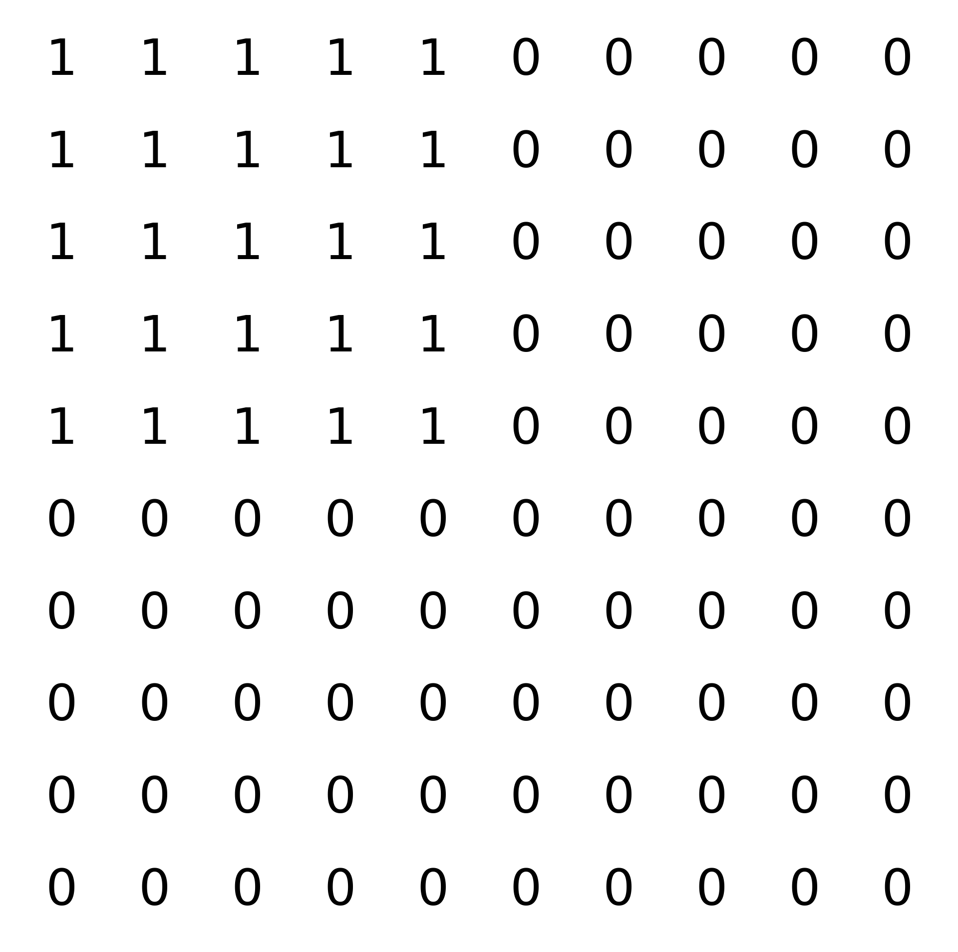
(a) TL

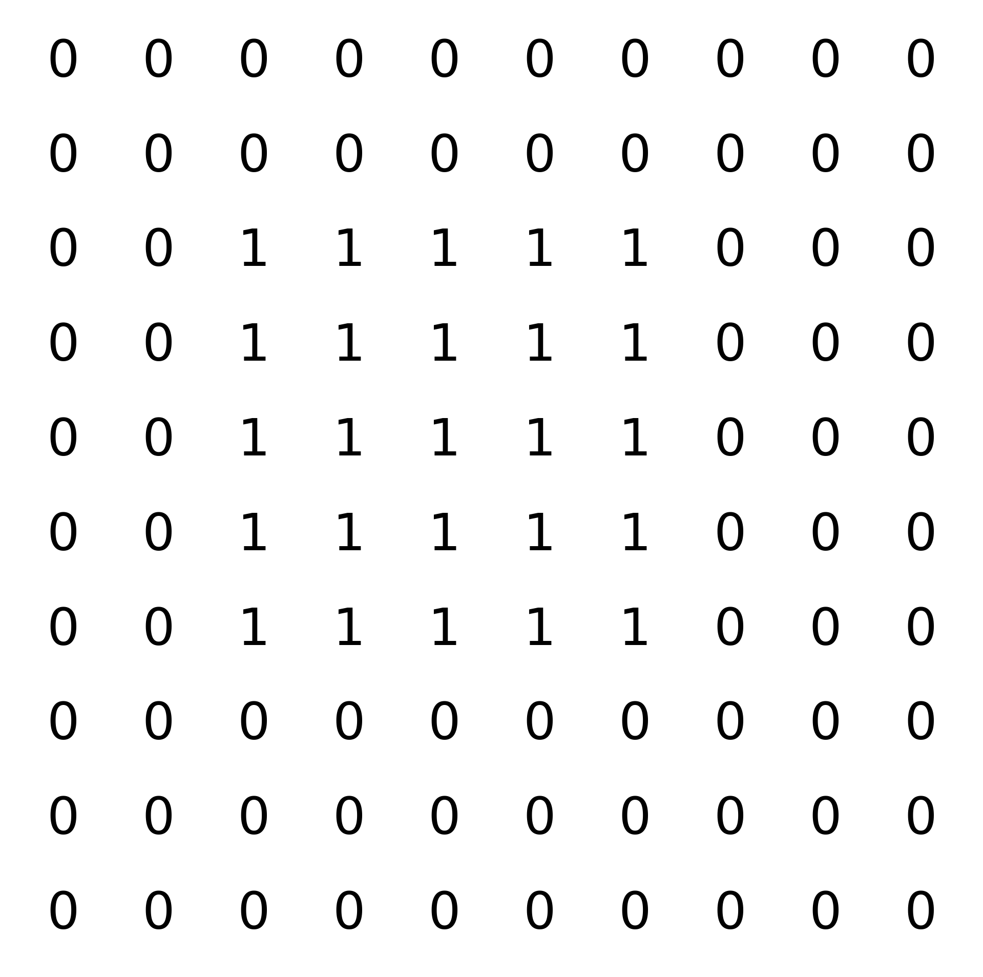
(b) CEN

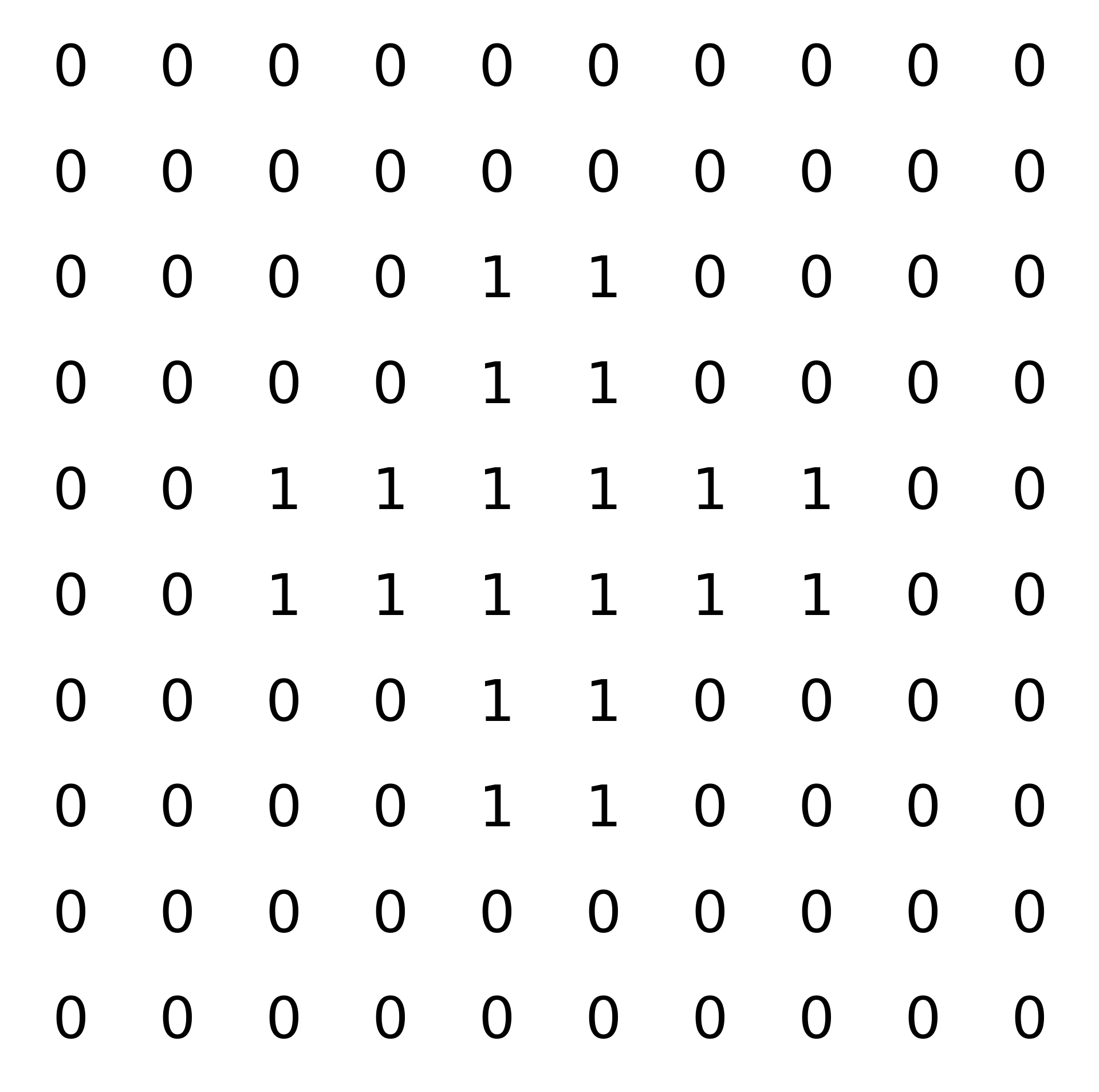
(c) CROSS

Figure 3: Ground truth images

For each image type, we consider two sizes: small-size $15\times 15$ images and medium-size $100\times 100$ images. To generate blurred images, as in [8], we employ the bit-flipping noise model defined in Section 1 with $p\in[0.1:0.1:0.5]$. For each fixed $p$, we generate 50 random instances and report average relative optimality gaps and average CPU times. All LPs and IPs are solved with Gurobi 11.0 where all options are set to their default values. The relative optimality gaps and CPU times for different LP relaxations are shown in Figure 4 and Figure 5, respectively. In all instances, the clique LP returns a binary solution; i.e., Problem cliqueLP solves the original nonconvex Problem B-UGM. Therefore, for this test set, there is no need to run the multi-clique LP. As can be seen from Figure 4, the standard LP performs poorly in all cases. The flower LP leads to a moderate improvement in the quality of bounds, while the running LP significantly outperforms the flower LP. However, Figure 5 indicates that the computational cost of solving running LP is significantly higher than other LP relaxations. Hence, for this test set, clique LP is the best relaxation as it always solves the original problem and has the lowest computational cost among competitors.

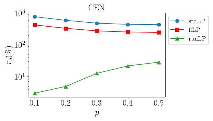
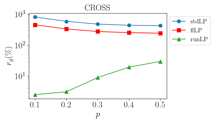
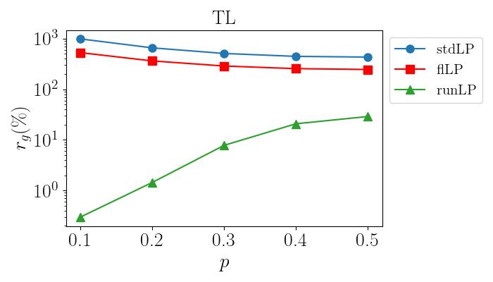
(a) $15\times 15$ images

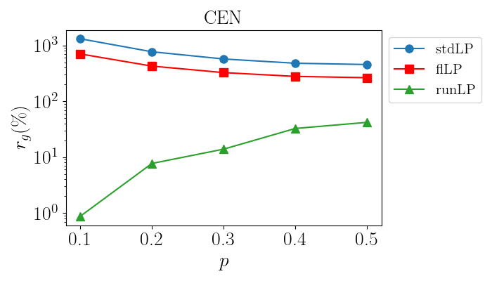
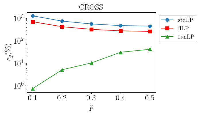
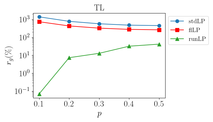
(b) $100\times 100$ images

Figure 4: Relative optimality gap of LPs for synthetic images.

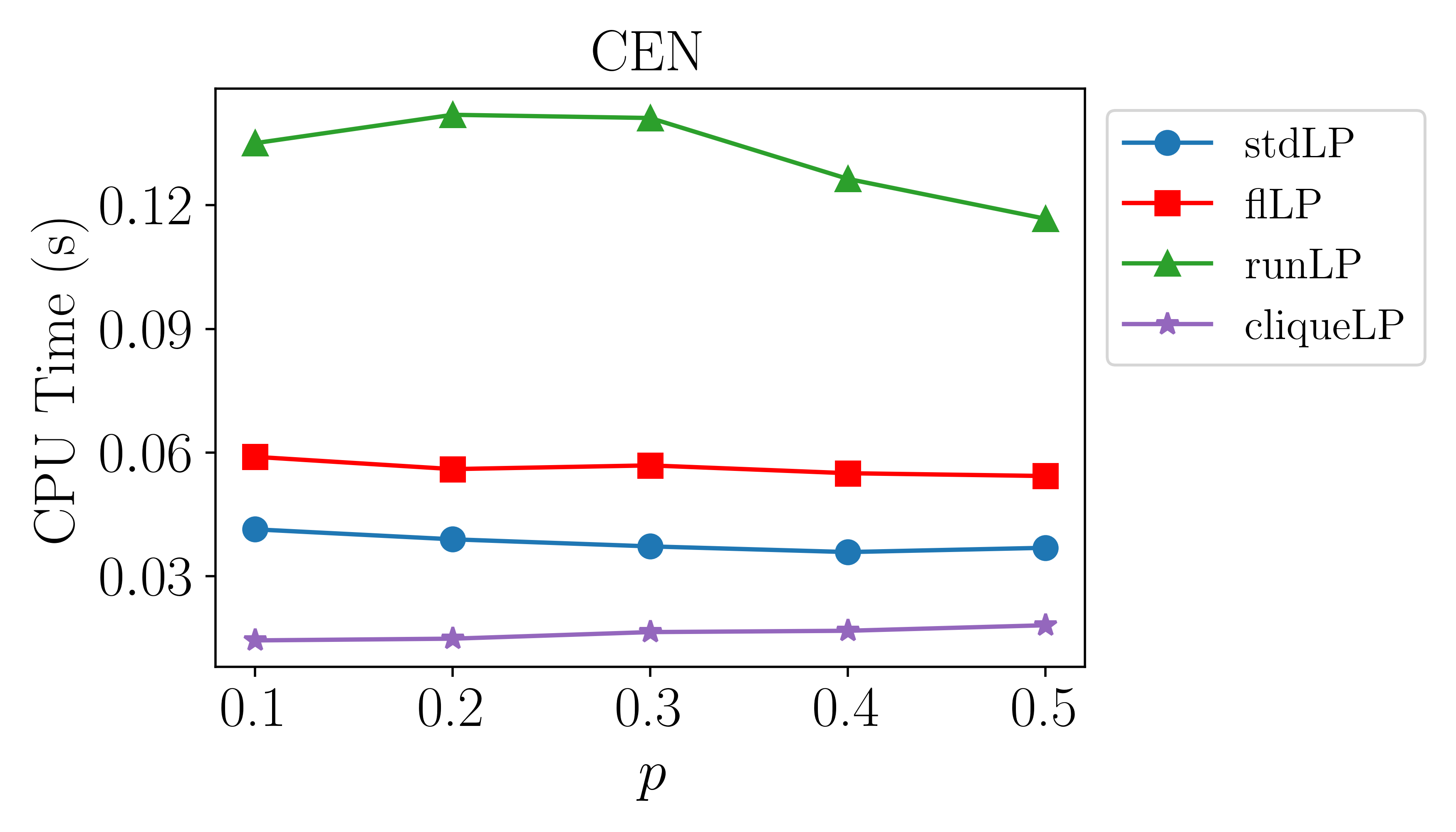
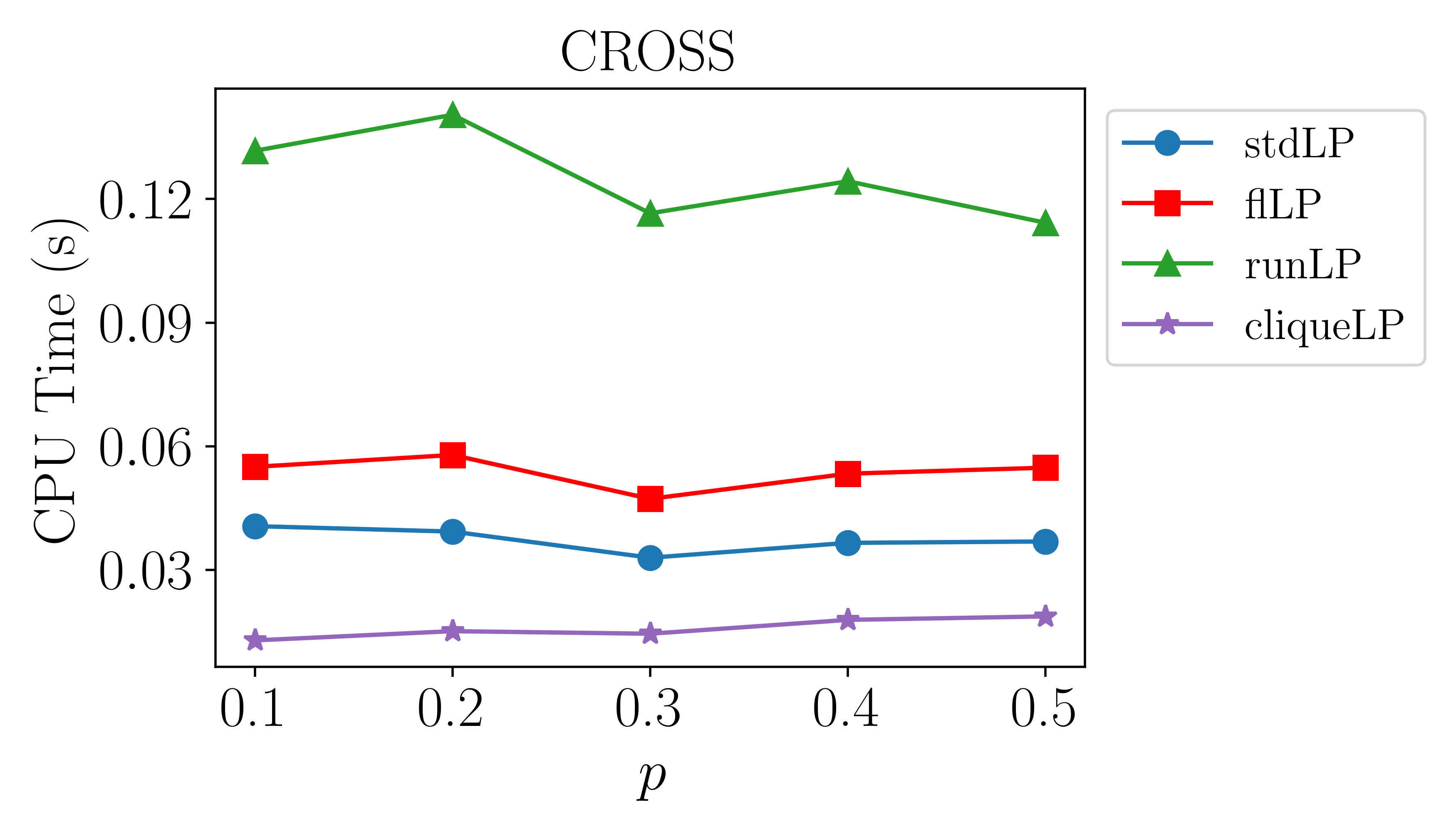
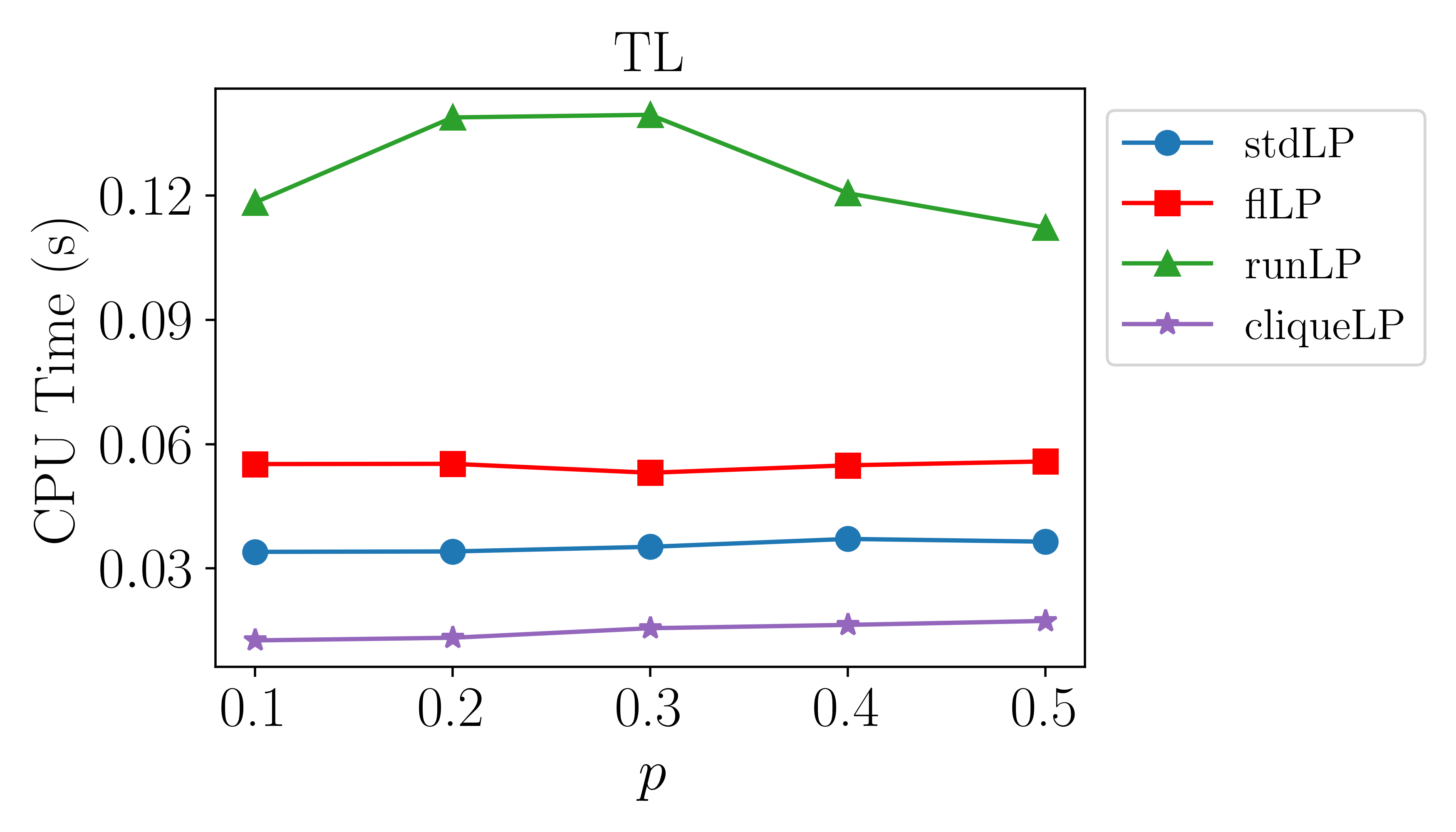
(a) $15\times 15$ images

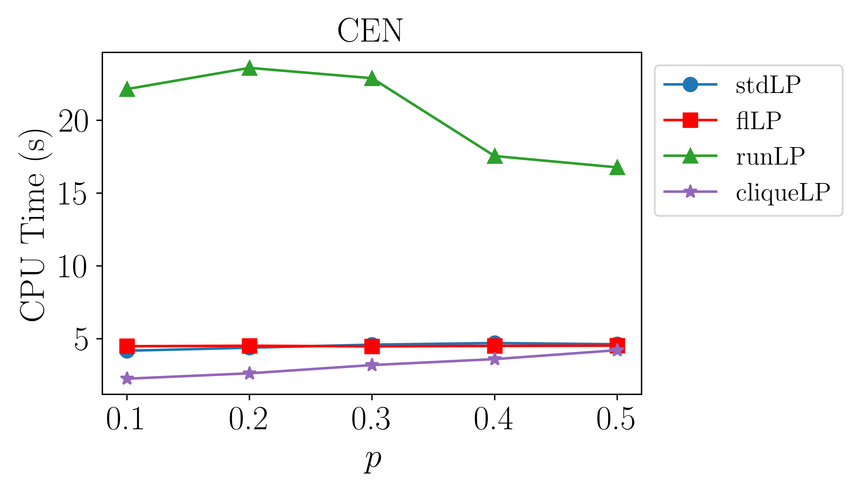
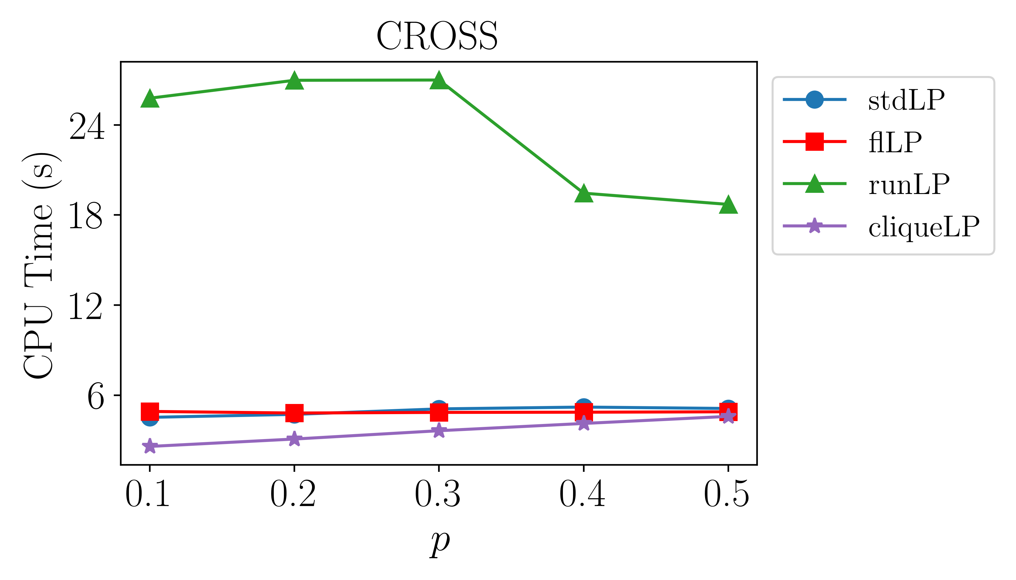
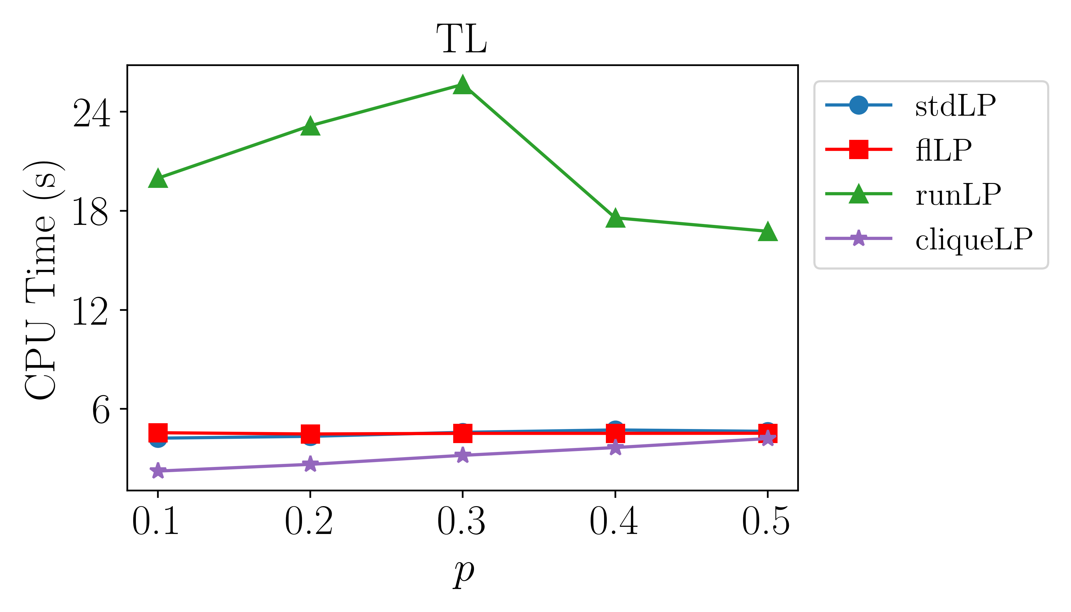
(b) $100\times 100$ images

Figure 5: CPU time of LP relaxations for synthetic images.

To illustrate the importance of constructing strong LP relaxations for Problem B-UGM, let us comment on the computational cost of solving the IP; as we mentioned before the IP is obtained by adding binary requirements for all variables to Problem stdLP. We consider a $100\times 100$ ground truth image of type CEN and for each $p\in[0.1:0.1:0.5]$ we generate a blurred image. We then use Gurobi 11.0 to solve the IP and we set the time limit to 1800 seconds. Results are summarized in Table 2; none of the IP instances are solved to optimality within the time limit; we also report the relative gap of the IP upon termination. As can be seen from the table, in all cases the relative gap is larger than $200\%$. Interestingly, in all cases clique LP returns a binary solution in less than $5$ seconds.

$p$	IP time (s)	gap $(\%)$	clique LP time (s)
$0.1$	$>1800$	$263$	$2.04$
$0.2$	$>1800$	$250$	$2.36$
$0.3$	$>1800$	$231$	$4.17$
$0.4$	$>1800$	$220$	$4.25$
$0.5$	$>1800$	$216$	$4.42$

Table 2: Performance of the IP for $100\times 100$ images of type CEN.

3.2 QR codes

In this section, we demonstrate the effectiveness of the proposed LPs to restore an important type of real-world images: QR Codes. To this end, we utilize a more systematic approach for setting parameters of the inference problem so that we examine the quality of restored images. Henceforth, given a ground truth image and an algorithm for solving the image restoration problem, we measure the quality of the restored image in terms of partial recovery; i.e., the fraction of pixels that are identical in ground truth and restored images. Whenever an LP returns a fractional solution, we first round the solution to the closest binary point and then compute the partial recovery.

To capture the smoothness information for QR codes, we choose to learn the potential values from small-size and “mildly blurred” images. That is, we generate $10$ distinct $50\times 50$ QR codes and we use the bit-flipping noise model with $p=0.05$ to generate midly blurred instances. Next, we compute the average fraction of times $f_{i}$, $i\in[4]$ each group listed in Table 1 appears in these images. We then set $\varphi_{i}=-f_{i}$ for all $i\in[4]$. While this method is unrealistic for real-world problems as it assumes we have the ground truth image at hand, it imitates practical approaches in which practitioners consider a large database of somewhat clean images to learn the frequency of different potential patterns. Using more sophisticated techniques to learn potential values is beyond the scope of this paper.

Next, we describe how to choose parameter $\alpha$; recall that $\alpha$ balances the similarity of the restored image to the blurred image and the smoothness of the restored image. We choose $\alpha$ that maximizes the average partial recovery over a set of small-size $50\times 50$ QR codes. More precisely, we generate $10$ distinct QR codes; for each ground truth image, we set $p\in\{0.1,0.2,0.3\}$ and for each fixed $p$ we generate 50 random blurred images. We set $\alpha\in[0.1:0.1:1.5]$ and for each fixed $\alpha$ we solve the IP. Notice that since we are considering $50\times 50$ QR codes, Gurobi is able to solve the IP in a few seconds. For each $(p,\alpha)$, we compute the average partial recovery over 50 instances and choose $\alpha$ that maximizes this quantity. Results are depicted in Figure 6; accordingly, we set $\alpha=1.0$ for our next tests.

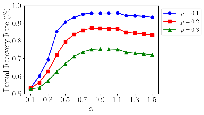
Figure 6: Learning parameter $\alpha$ using $50\times 50$ QR codes

To test the performance of the proposed LP relaxations for restoring QR codes, we construct as the ground truth a $200\times 200$ QR code which contains a $100$-character-long text string. We set $p\in[0.1:0.1:0.5]$ and for each fixed $p$, we generate $50$ random instances. Results are shown in Figure 7. In addition to partial recovery rate, relative optimality gap, and CPU time, we also compare the tightness rate of different LPs; we define the tightness rate as the fraction of times each LP returns a binary solution. As can be seen from these figures, for this test set, standard LP and flower LP perform quite poorly, whereas, running LP, clique LP and multi-clique LP perform very well. Namely, the partial recovery rate of these three LPs is very close to that of the IP. Interestingly, multi-clique LP has the best tightness rate; however, in many instances for which running LP and clique LP return fractional solutions, the relative optimality gaps are very small, and the rounded binary solutions lead to similar partial recovery values to those of multi-clique LP. As before, the computational cost of solving running LP is significantly higher than other LPs. Hence for this test set multi-clique LP is the best option, followed closely by the clique LP.

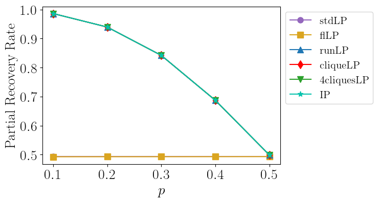
(a) Partial recovery rate

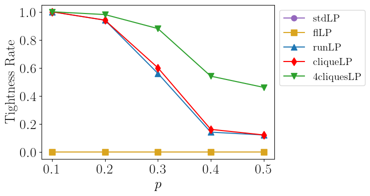
(b) Tightness rate

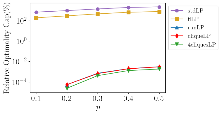
(c) Relative optimality gap

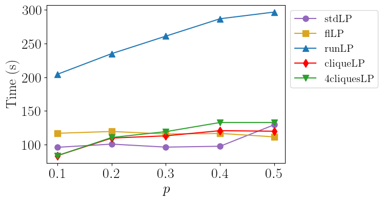
(d) CPU time (s)

Figure 7: Performance of different LPs for restoring QR codes

Figure 8 shows the $200\times 200$ ground truth QR code, together with a noisy instance with $p=0.2$ and the restored QR code obtained by solving the clique LP. While the noisy QR code (Figure 8(b)) does not scan, the restored QR code (Figure 8(c)) scans successfully.

(a) original

(b) $p=0.2$

(c) restored

Figure 8: Restoring QR codes with LP relaxations.

4 Second application: decoding error-correcting codes

Transmitting a message, represented as a sequence of binary numbers, across a noisy channel is a central problem in information theory. The received message is often different from the original one due to the presence of noise in the channel and the goal in decoding is to recover the ground truth message. To this end, a common strategy is to transmit some redundant bits along with the original message, containing additional information about the message, so that some of the errors can be corrected. Such messages are often referred to as error-correcting codes. Low Density Parity Check (LDPC) codes, first introduced by Gallager [24], are a popular type of error-correcting codes in which additional information is transmitted via parity bits; it has been shown that LDPC codes enjoy various desirable theoretical and computational properties [37, 20, 19]. Existing methods for decoding LDPC codes are based on the belief propagation algorithm [34] and LP relaxations [20, 19].

LDPC codes are often represented via UGMs; namely, each node of the graph corresponds to a message bit while each clique corresponds to a subset of bits with even parity. Gallager [24] introduced LDPC codes as error-correcting codes with three properties: $(i)$ all cliques have the same cardinality, denoted by $\beta$, $(ii)$ each node appears in the same number of cliques, denoted by $\gamma$, and $(iii)$ $\beta>\gamma$. Denoting by $n$ the number of message bits, an LDPC code is fully characterized by the triplet $(n,\beta,\gamma)$. Figure 9 illustrates an LDPC code.

Figure 9: The clique structure of a $(9,3,2)$ LDPC code.

Now let us formalize the problem of decoding LDPC codes. Consider a ground truth message $x_{v}$, $v\in V$. Denote by $\oplus$ the addition in modulo two arithmetic. Then for each $C\in{\mathcal{C}}$ we must have $\oplus_{v\in C}{z_{v}}=1$. That is, we define the clique potentials $\phi_{C}(z_{C})$, $C\in{\mathcal{C}}$ as follows:

$$\phi_{C}(z_{C})=\left\{\begin{array}[]{ll}1&{\rm if}\;\oplus_{v\in C}{z_{v}}=1\\ 0&{\rm otherwise.}\end{array}\right.$$

The above expression in turn can be equivalently written as:

$$\phi_{C}(z_{C})=\sum_{\begin{subarray}{c}S\subseteq C\\ |S|\;{\rm even}\end{subarray}}{\Big{(}\prod_{v\in S}{z_{v}}\prod_{v\in C\setminus S}{(1-z_{v})}\Big{)}}.$$

Denoting the noisy message by $y_{v}$, $v\in V$ and assuming the bit-flipping model for the noisy channel, we deduce that the decoding problem for an LDPC code can be written as:

$${\rm max}\quad \sum_{\begin{subarray}{c}v\in V:\\ y_{v}=1\end{subarray}}{z_{v}}-\sum_{\begin{subarray}{c}v\in V:\\ y_{v}=0\end{subarray}}{z_{v}}$$ (DCD)

$${\rm s.t.} \sum_{\begin{subarray}{c}S\subseteq C\\ |S|\;{\rm even}\end{subarray}}{\Big{(}\prod_{v\in S}{z_{v}}\prod_{v\in C\setminus S}{(1-z_{v})}\Big{)}}=1,\quad\forall C\in{\mathcal{C}}$$

$$z_{v}\in\{0,1\},\forall v\in V.$$

Denote by ${\mathcal{D}}({\mathcal{C}})$ the feasible region of Problem DCD. As before we introduce auxiliary variables $z_{e}:=\prod_{v\in e}{z_{v}}$ for all $e\in\bar{P}(C)$ and $C\in{\mathcal{C}}$ to obtain the following reformulation of Problem DCD in an extended space:

$${\rm max}\quad \sum_{\begin{subarray}{c}v\in V:\\ y_{v}=1\end{subarray}}{z_{v}}-\sum_{\begin{subarray}{c}v\in V:\\ y_{v}=0\end{subarray}}{z_{v}}$$ (L-DCD)

$${\rm s.t.}\quad \sum_{\begin{subarray}{c}p\subseteq C:\\ p\neq\emptyset\end{subarray}}{(-2)^{|p|-1}z_{p}}=0,\quad\forall C\in{\mathcal{C}}$$

$$z\in S({\mathcal{G}}),$$

where $S({\mathcal{G}})$ is the multilinear set of the UGM hypergraph ${\mathcal{G}}=(V,{\mathcal{E}})$, ${\mathcal{E}}=\cup_{C\in{\mathcal{C}}}{\bar{P}(C)}$ and is defined by (7). By replacing the nonconvex set $S({\mathcal{G}})$ in $z\in S({\mathcal{G}})$ with the polyhedral relaxations introduced in Section 2, we obtain various LP relaxations for Problem L-DCD. In the following, we denote by $S^{e}({\mathcal{G}})$ the feasible region of Problem L-DCD and by $\text{MP}^{e}({\mathcal{G}})$ its convex hull.

4.1 The clique relaxation for decoding

The clique LP for Problem L-DCD is obtained by replacing the constraint $z\in S({\mathcal{G}})$ with $z\in\text{MP}^{\rm cl}({\mathcal{G}})$, where $\text{MP}^{\rm cl}({\mathcal{G}})$ is the clique relaxation and is defined in Section 2.4. In the following, we show that clique LP for Problem L-DCD has an interesting interpretation; namely, it is obtained by replacing the feasible region of Problem L-DCD corresponding to a single clique $C$ with its convex hull.

Proposition 7.

Let ${\mathcal{G}}_{C}$ denote the complete hypergraph with node set $C$. Consider the set

$$S^{e}({\mathcal{G}}_{C})=\Big{\{}z\in S({\mathcal{G}}_{C}):\sum_{\begin{subarray}{c}p\subseteq C:\\ p\neq\emptyset\end{subarray}}{(-2)^{|p|-1}z_{p}}=0\Big{\}}.$$

Then the convex hull of $S^{e}({\mathcal{G}}_{C})$ is given by:

$$\text{MP}^{e}({\mathcal{G}}_{C})=\Big{\{}z\in\text{MP}({\mathcal{G}}_{C}):\sum_{\begin{subarray}{c}p\subseteq C:\\ p\neq\emptyset\end{subarray}}{(-2)^{|p|-1}z_{p}}=0\Big{\}}.$$ (31)

Proof.

To prove the statement, it suffices to show that $\text{MP}^{e}({\mathcal{G}}_{C})$ is an extended formulation for the convex hull of the set:

$${\mathcal{D}}(C):=\Big{\{}z\in\{0,1\}^{C}:\sum_{\begin{subarray}{c}S\subseteq C\\ |S|\;{\rm even}\end{subarray}}{\Big{(}\prod_{v\in S}{z_{v}}\prod_{v\in C\setminus S}{(1-z_{v})}\Big{)}}=1\Big{\}}.$$

To construct the convex hull of ${\mathcal{D}}(C)$ we make use of RLT as defined in [39]. That is, let $J_{1},J_{2}$ be any partition of $C$; define the factor $F(J_{1},J_{2})=\prod_{v\in J_{1}}{z_{v}}\prod_{v\in J_{2}}{(1-z_{v})}$. We first expand each $F(J_{1},J_{2})\geq 0$ and let $z_{e}=\prod_{v\in e}{z_{v}}$ for each product term to obtain linear inequalities (18). Subsequently, we multiply the equality constraint

$$\sum_{\begin{subarray}{c}S\subseteq C\\ |S|\;{\rm even}\end{subarray}}{\Big{(}\prod_{v\in S}{z_{v}}\prod_{v\in C\setminus S}{(1-z_{v})}\Big{)}}=1,$$ (32)

by each factor $F(J_{1},J_{2})$ and let $z_{e}=\prod_{v\in e}{z_{v}}$ to obtain a collection of linear equalities. Let us examine these equalities; two cases arise:

• if $|J_{1}|$ is even, then multiplying $F(J_{1},J_{2})$ by equality (32) and using $z_{v}(1-z_{v})=0$ for any $v\in C$, we obtain the trivial equality $F(J_{1},J_{2})=F(J_{1},J_{2})$.

• if $|J_{1}|$ is odd, then multiplying $F(J_{1},J_{2})$ by equality (32) and using $z_{v}(1-z_{v})=0$ for any $v\in C$, we obtain $F(J_{1},J_{2})=0$.

Therefore, by Section 4 of [39], the following system defines an extended formulation for the convex hull of ${\mathcal{D}}(C)$:

$$\psi_{U}(z_{C})\geq 0,\;\forall U\subseteq C:|U|\;{\rm even},\;\psi_{U}(z_{C})=0,\;\forall U\subseteq C:|U|\;{\rm odd},$$

where $\psi_{U}(z_{C})$ is defined by (19). To complete the proof, it suffices to show that $\psi_{U}(z_{C})\geq 0$ for all $U\subseteq C$ together with

$$\sum_{p\subseteq C,p\neq\emptyset}{(-2)^{|p|-1}z_{p}}=0,$$ (33)

implies $\psi_{U}(z_{C})=0$ for all $U\subseteq C$ such that $|U|$ is odd. To see this, first note that (33) can be equivalently written as $\sum_{U\subseteq C:|U|{\rm even}}{\psi_{U}(z_{C})}=1$. Moreover, from the definition of $\psi_{U}(z_{C})$ we have $\sum_{U\subseteq C}{\psi_{U}(z_{C})}=1$. These two inequalities imply $\sum_{U\subseteq C:|U|{\rm odd}}{\psi_{U}(z_{C})}=0$, which together with $\psi_{U}(z_{C})\geq 0$ for all $U\subseteq C$ yield $\psi_{U}(z_{C})=0$ for all $U\subseteq C$ such that $|U|$ is odd. ∎

4.2 The parity polytope and the parity LP

In [29], Jeroslow proved that the convex hull of the set of binary vectors $x\in\{0,1\}^{n}$ with even parity, denoted by ${\mathcal{P}}_{n}$, is given by:

$${\mathcal{P}}_{n}=\Big{\{}x\in[0,1]^{n}:\sum_{i\in S}{(1-x_{i})}+\sum_{i\in[n]\setminus S}{x_{i}}\geq 1,\;\forall S\subseteq[n]:|S|\;\text{is odd}\Big{\}}.$$ (34)

Using this characterization, the authors of [20], introduced the following LP relaxation of Problem DCD, which we will refer to as the parity LP:

$${\rm max}\quad \sum_{\begin{subarray}{c}v\in V:\\ y_{v}=1\end{subarray}}{z_{v}}-\sum_{\begin{subarray}{c}v\in V:\\ y_{v}=0\end{subarray}}{z_{v}}$$ (parLP)

$${\rm s.t.}\quad \sum_{v\in S}{(1-z_{v})}+\sum_{v\in C\setminus S}{z_{v}}\geq 1,\quad\forall S\subseteq C:|S|\;\text{is odd},\;\forall C\in{\mathcal{C}}$$

$$z_{v}\in[0,1],\forall v\in V.$$

In the following we show that clique LP is stronger than parity LP, in general. Denote by ${\mathcal{P}}({\mathcal{C}})$ the feasible region of Problem parLP. If ${\mathcal{C}}$ consists of a single clique $C$, then by Proposition 7:

$${\mathcal{P}}(C)={\rm proj}_{z_{v},v\in C}(\text{MP}^{e}({\mathcal{G}}_{C}))={\rm proj}_{z_{v},v\in C}(\text{MP}({\mathcal{G}}_{C})\cap{\mathcal{H}}_{C}),$$

where ${\mathcal{H}}_{C}$ denotes the set of points satisfying equality (33). This implies that the feasible region of clique LP is contained in the feasible region of parity LP. As we detail next, this containment is often strict. We first examine the strength of clique LP. In [15], the authors generalize the decomposition result of Theorem 1 to account for additional constraints on multilinear sets:

Theorem 2 (Corollary 1 in [15]).

Let ${\mathcal{G}}$ be a hypergraph, and let ${\mathcal{G}}_{1}$,${\mathcal{G}}_{2}$ be section hypergraphs of ${\mathcal{G}}$ such that ${\mathcal{G}}_{1}\cup{\mathcal{G}}_{2}={\mathcal{G}}$ and ${\mathcal{G}}_{1}\cap{\mathcal{G}}_{2}$ is a complete hypergraph. Let $C({\mathcal{G}})$ be the set of points in $S({\mathcal{G}})$ that satisfy a number of constraints, each one containing only variables corresponding to nodes and edges only in ${\mathcal{G}}_{1}$ or only in ${\mathcal{G}}_{2}$. For $i=1,2$, let $C({\mathcal{G}}_{i})$ be the projection of $C({\mathcal{G}})$ in the space of $S({\mathcal{G}}_{i})$. Then, $C({\mathcal{G}})$ is decomposable into $C({\mathcal{G}}_{1})$ and $C({\mathcal{G}}_{2})$.

Thanks to Theorem 2 and Proposition 7, we can employ a similar line of arguments as in the proof of Proposition 4 to obtain a sufficient condition for sharpness of clique LP for decoding:

Proposition 8.

Let ${\mathcal{G}}=\cup_{C\in{\mathcal{C}}}{{\mathcal{G}}_{C}}$ where ${\mathcal{G}}_{C}$ is a complete hypergraph with node set $C$. If ${\mathcal{C}}$ has the running intersection property, then

$$\text{MP}^{e}({\mathcal{G}})=\bigcap_{C\in{\mathcal{C}}}(\text{MP}({\mathcal{G}}_{C})\cap{\mathcal{H}}_{C}).$$

If ${\mathcal{C}}=\{C_{1},C_{2}\}$, then ${\mathcal{C}}$ clearly has the running intersection property. However, as we show next, even in this case the parity relaxation ${\mathcal{P}}({\mathcal{C}})$ does not coincide with the convex hull.

Example 1.

Let ${\mathcal{C}}=\{C_{1},C_{2}\}$ with $C_{1}=\{v_{1},v_{2},v_{3},v_{4}\}$ and $C_{2}=\{v_{3},v_{4},v_{5},v_{6}\}$. It can be checked that the point $\tilde{z}_{v_{1}}=\tilde{z}_{v_{2}}=\tilde{z}_{v_{5}}=0$, $\tilde{z}_{v_{3}}=\tilde{z}_{v_{4}}=\frac{1}{2}$ and $\tilde{z}_{v_{6}}=1$ is feasible for ${\mathcal{P}}({\mathcal{C}})$. Since the points in $C_{1}$ and $C_{2}$ should have even parity, we conclude that the points in $(C_{1}\setminus C_{2})\cup(C_{2}\setminus C_{1})$ should have even parity as well; that is, inequality $(1-z_{v_{6}})+z_{v_{1}}+z_{v_{2}}+z_{v_{5}}\geq 1$ is valid for ${\mathcal{D}}({\mathcal{C}})$. Substituting $\tilde{z}$ in this inequality yields $1-1+0+0+0\not\geq 1$, implying that ${\mathcal{D}}({\mathcal{C}})$ is strictly contained in ${\mathcal{P}}({\mathcal{C}})$.

4.3 Numerical Experiments

In this section, we compare the performance of different LP relaxations for decoding LDPC codes. We first describe how LDPC codes are generated [24]: an $(n,\beta,\gamma)$ LDPC code is often characterized by a parity-check matrix, an $m\times n$ binary matrix with $m:=\frac{n}{\gamma}\times\beta$, where each row contains $\beta$ ones and each column contains $\gamma$ ones. To construct a parity check matrix, we start by creating a matrix with all ones arranged in descending order; the $i$th row contains ones in columns $(i-1)\beta+1$ to $i\beta$. We then permute the columns of this matrix randomly and append it to the initial matrix. This permutation and appending is repeated $\gamma-1$ times to ensure each column contains $\gamma$ ones. The ones in each row of the matrix then correspond to the nodes of a clique in the UGM. It then follows that the UGM consists of $\frac{n}{\gamma}\times\beta$ cliques, each consisting of $\beta$ nodes. We assume an all-zero code as the ground truth code. As the first set of experiments, we consider a $(60,4,3)$ LDPC code. We use the bit-flipping noise with $p\in[0:0.01:0.2]$ and for each $p$ we generate $400$ random trials. We then compare the performance of different LPs with respect to tightness rate and partial recovery rate as defined before. For the multi-clique LP we set $m=4$; i.e., in our tests lifted odd-cycle inequalities (6) for cycles of cliques of length three and four are generated. Results are shown in Figure 10. As can be seen from this figure, standard LP and flower LP perform quite poorly, while running LP, clique LP, multi-clique LP, and parity LP perform well. Multi-clique LP is the best, followed by clique LP, followed by running LP, followed by the parity LP. As before the computational cost of solving running LP is significantly higher than other LPs. Motivated by these observations, in the next set of experiments we restrict our study to parity LP, clique LP, and multi-clique LP.

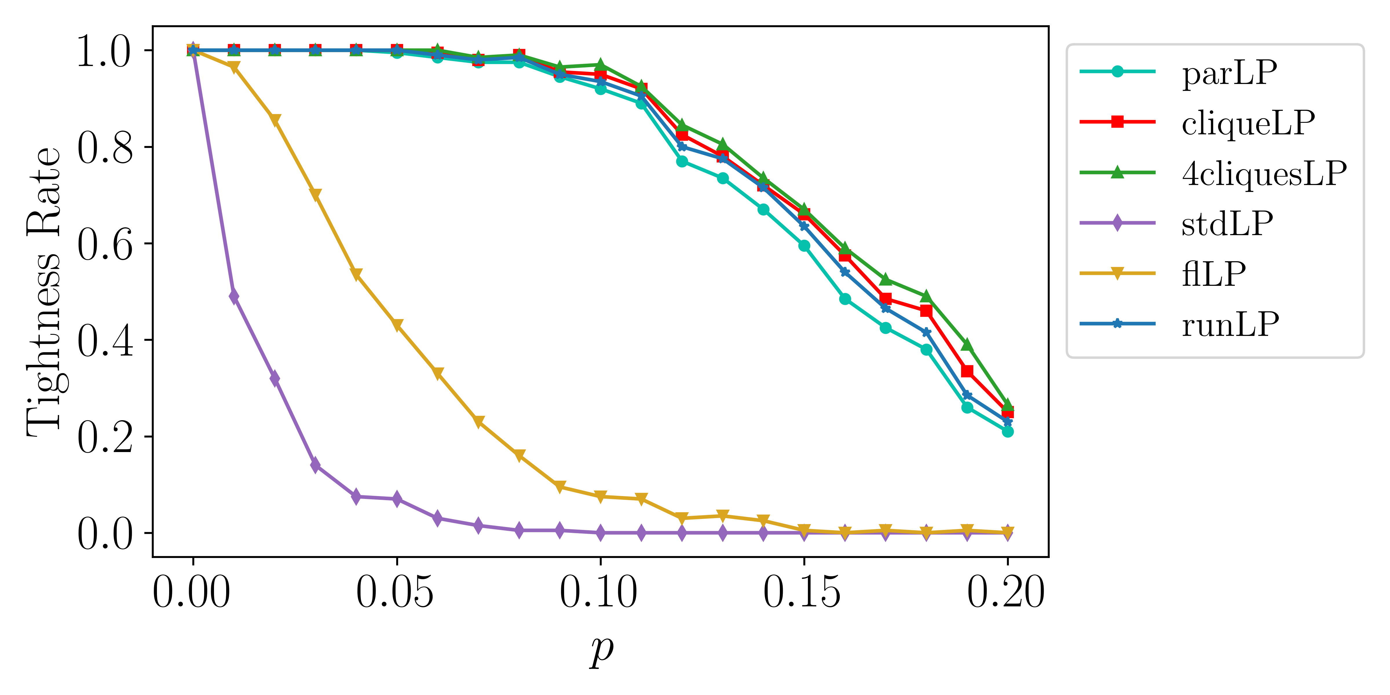
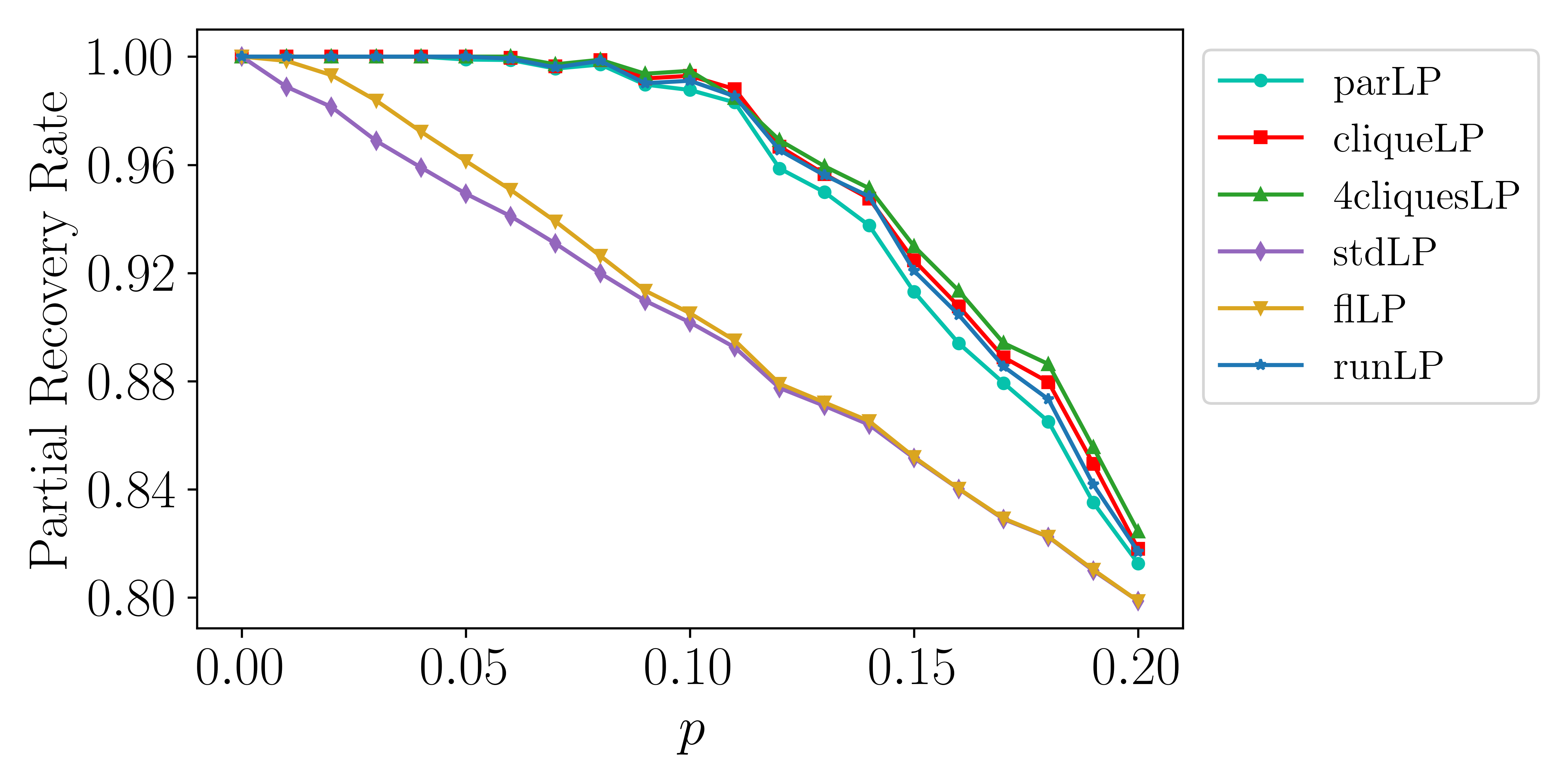
Figure 10: Performance of different LPs for decoding $(60,4,3)$ LDPC codes.

We next consider three type of LDPC codes: $(120,4,3)$, $(120,5,4)$, and $(120,6,5)$. We set $p\in[0:0.01:0.2]$ and for each $p$ we generate $400$ random trials. Results are depicted in Figure 11. Overall, multi-clique LP and clique LP have better tightness rates than the parity LP, as the theory suggests. However, the differences, specially in terms of partially recovery rates become smaller as we increase the code length. This indeed, indicates the difficulty of solving this problem class; namely, by constructing stronger LP relaxations, the partial recovery rate of the decoder only marginally improves. These results also suggest that for a fixed code length, as we increase the clique size, the performance of all LPs degrade; while for a $(120,4,3)$ LDPC code all LPs manage to recover the ground truth with up to about $10\%$ corruption, for a $(120,6,5)$ LDPC code, this number decreases to about $5\%$ corruption.

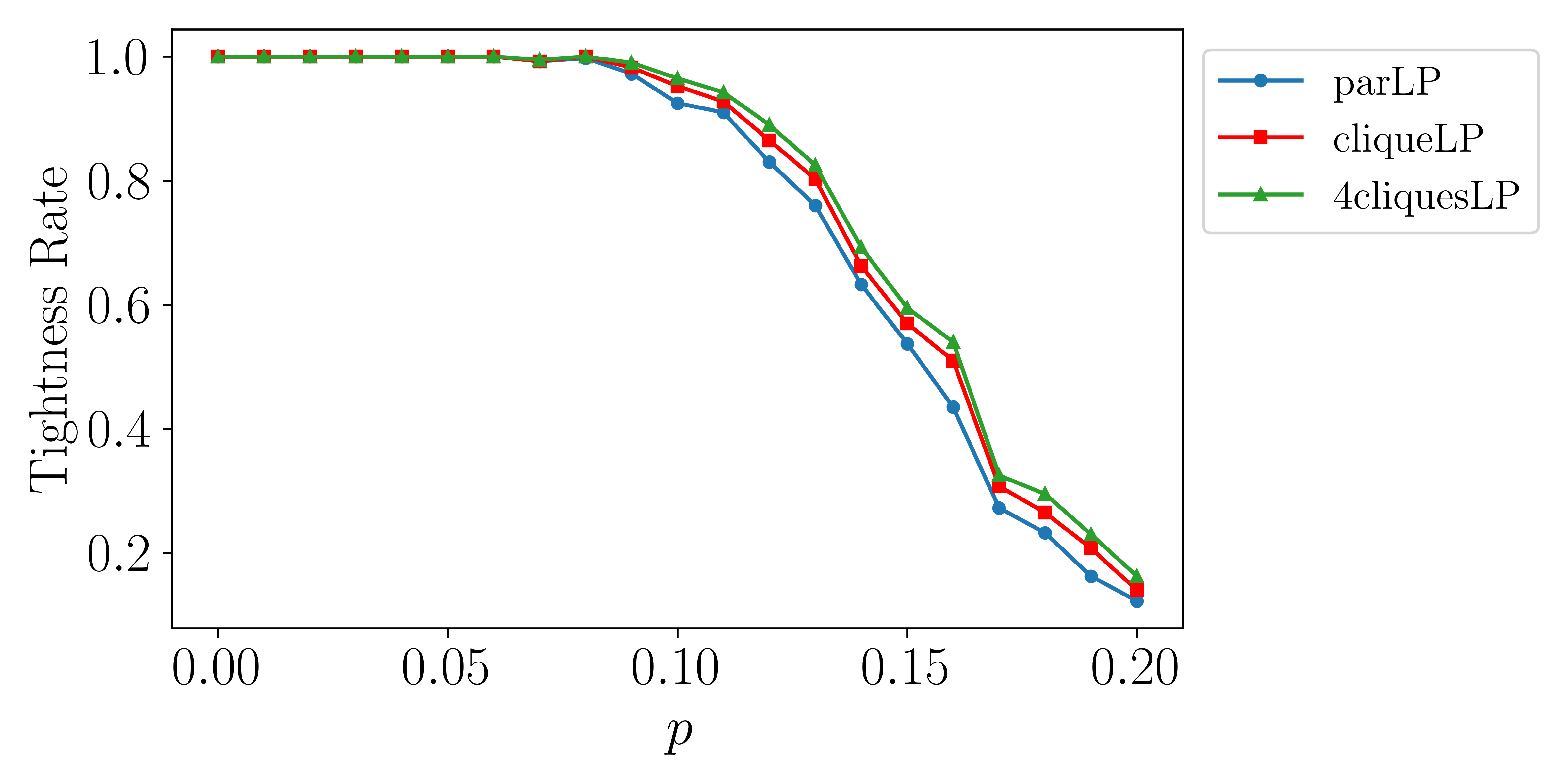
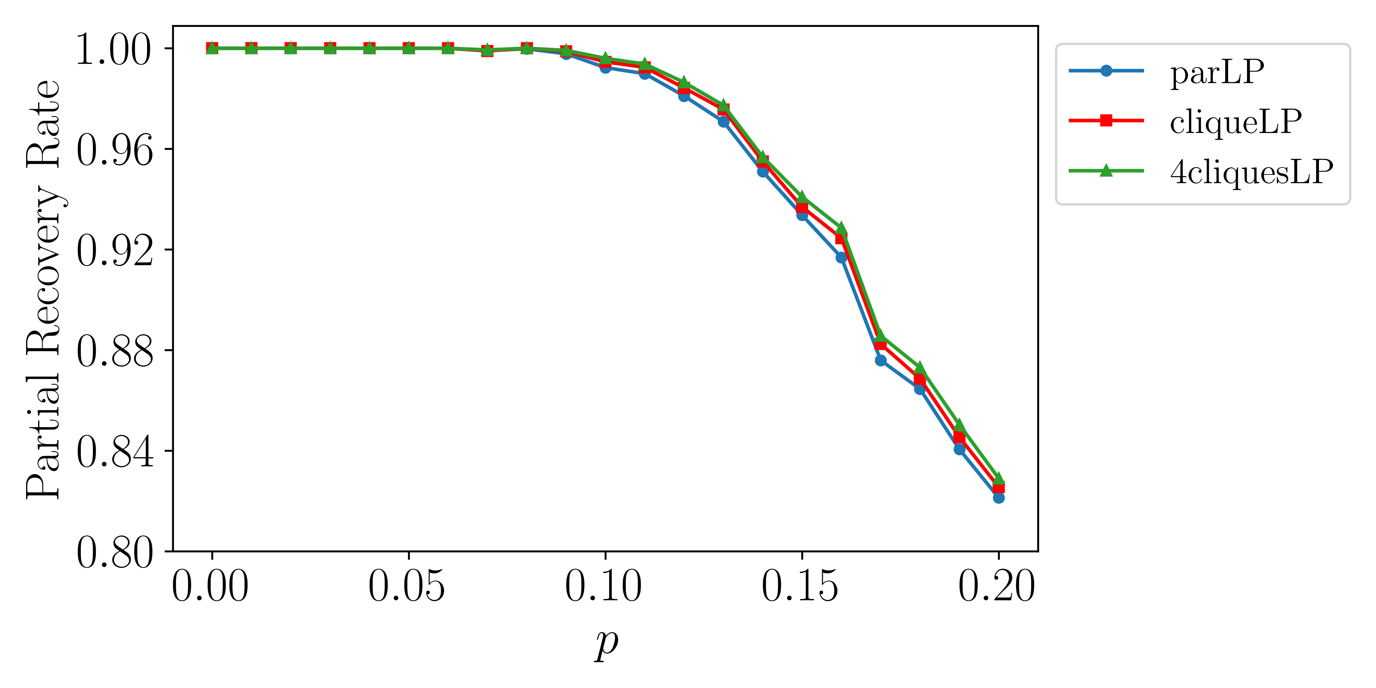
(a) $(120,4,3)$ LDPC codes

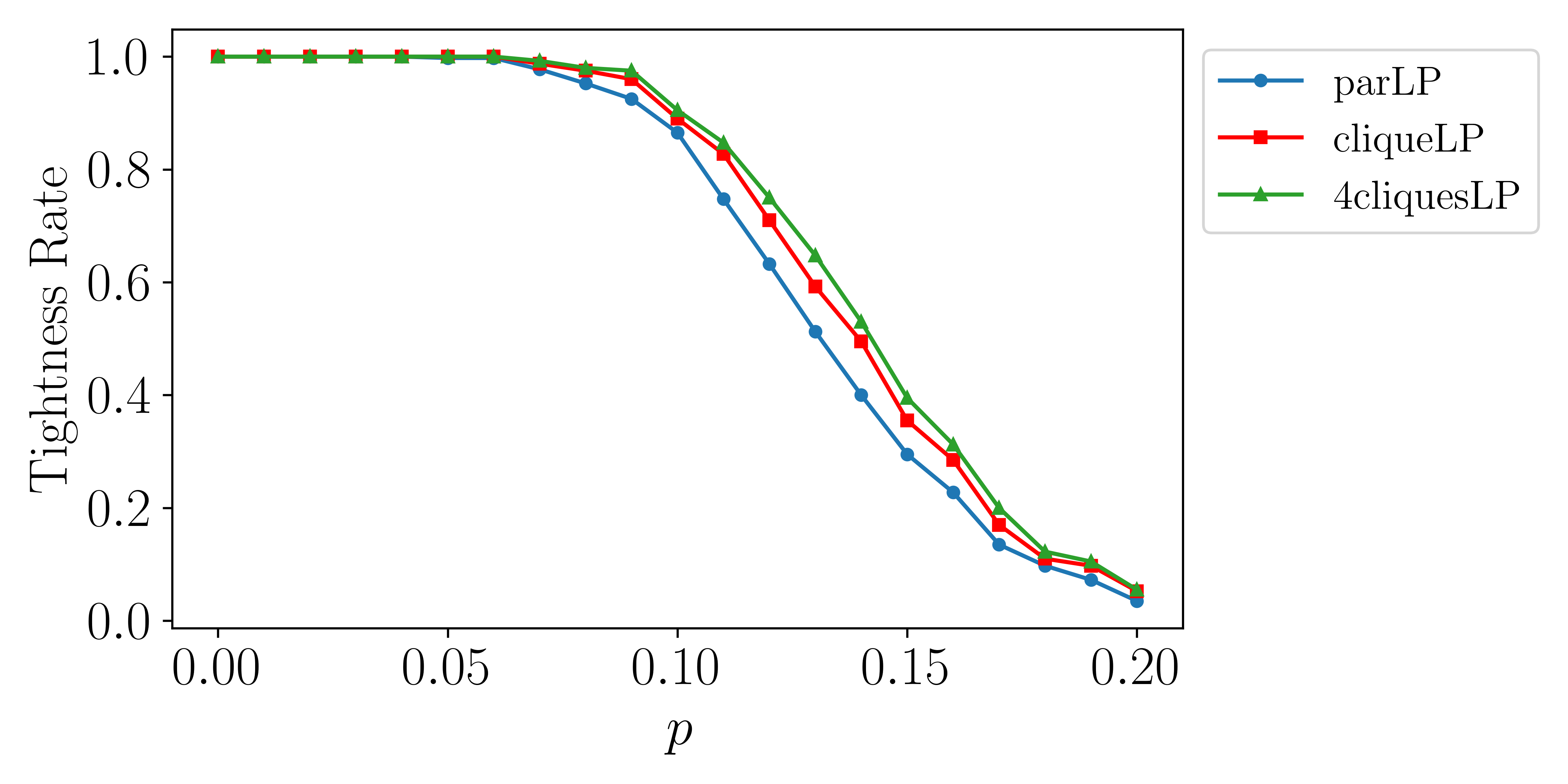
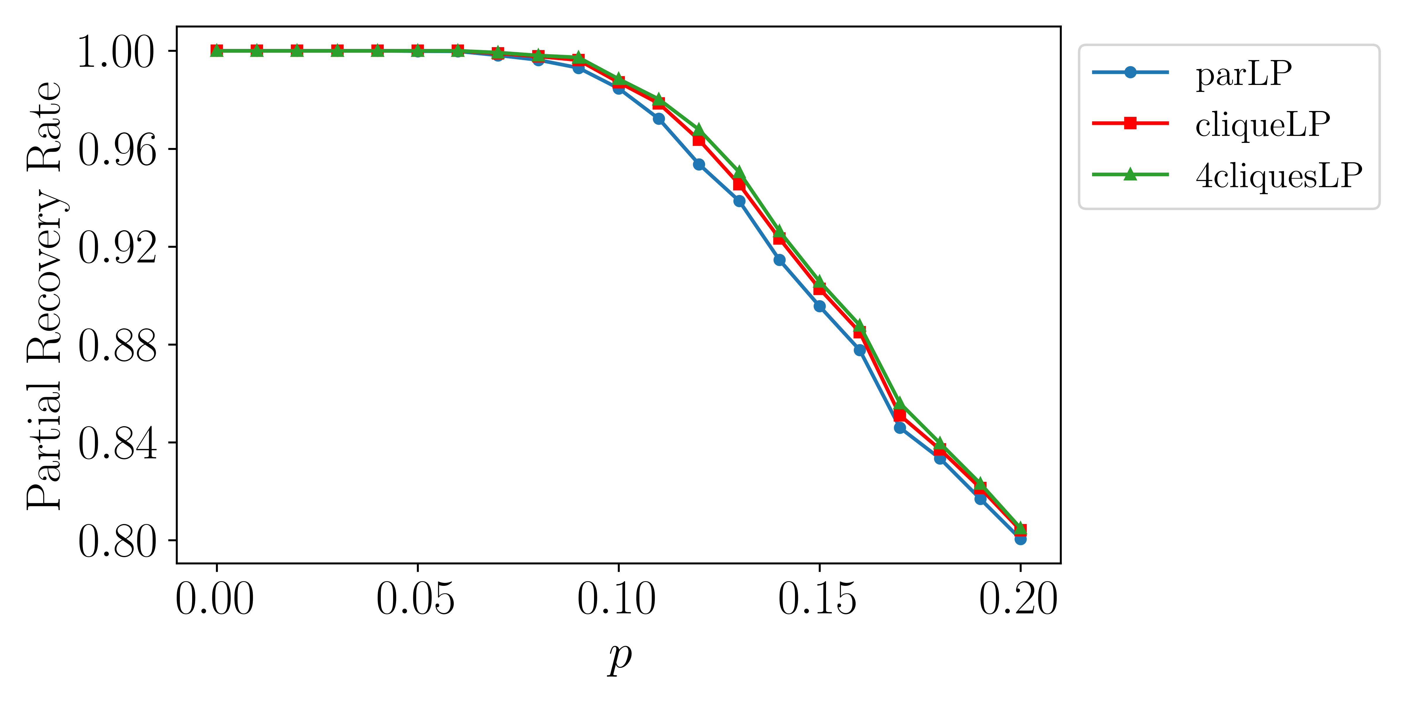
(b) $(120,5,4)$ LDPC codes

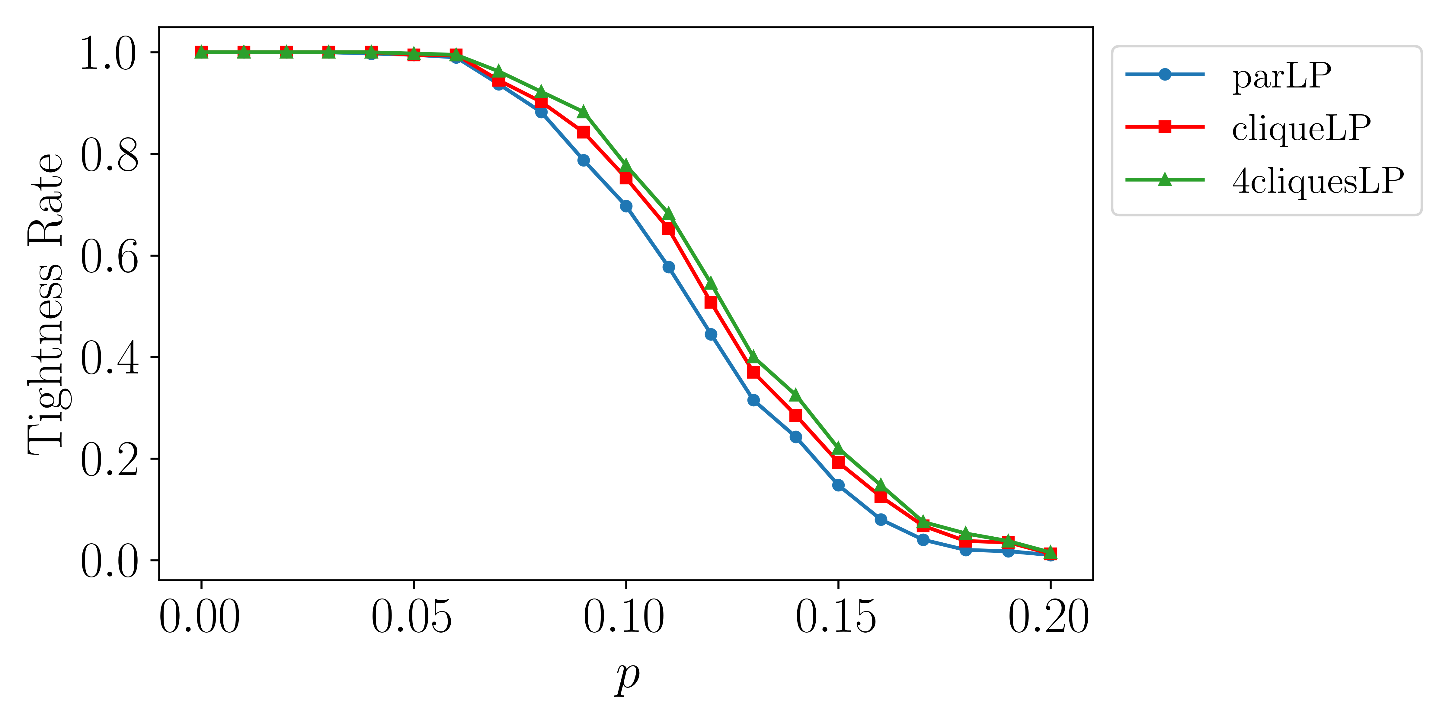
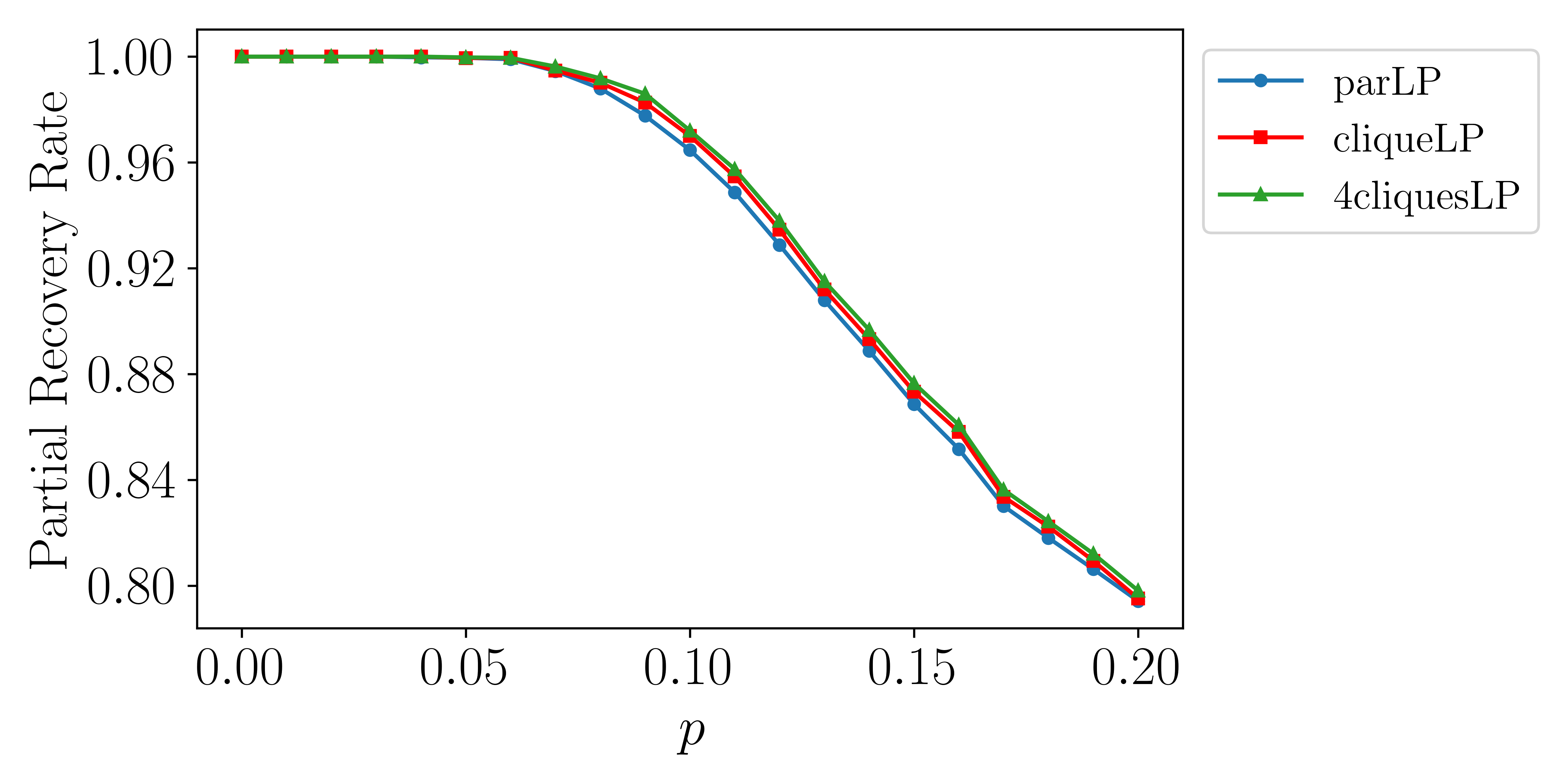
(c) $(120,6,5)$ LDPC codes

Figure 11: Performance of LP relaxations for decoding longer LDPC codes.

References

- [1] A. M. Ali, A. A. Farag, and G. L. Gimel’Farb. Optimizing binary MRFs with higher order cliques. In European Conference on Computer Vision, pages 98–111. Springer, 2008.
- [2] E. Balas. Disjunctive programming: Properties of the convex hull of feasible points. Discrete Applied Mathematics, 89(1-3):3–44, 1998.
- [3] C. Beeri, R. Fagin, D. Maier, and M. Yannakakis. On the desirability of acyclic database schemes. Journal of the ACM, 30:479–513, 1983.
- [4] Y. Boykov and G. Funka-Lea. Graph cuts and efficient ND image segmentation. International journal of computer vision, 70(2):109–131, 2006.
- [5] Y. Boykov, O. Veksler, and R. Zabih. Fast approximate energy minimization via graph cuts. IEEE Transactions on pattern analysis and machine intelligence, 23(11):1222–1239, 2001.
- [6] C. Buchheim, Y. Crama, and E. Rodríguez-Heck. Berge-acyclic multilinear optimization problems. European Journal of Operational Research, 2018.
- [7] Y. Crama. Concave extensions for non-linear maximization problems. Mathematical Programming, 61(1):53–60, 1993.
- [8] Y. Crama and E. Rodríguez-Heck. A class of valid inequalities for multilinear 0–1 optimization problems. Discrete Optimization, 25:28–47, 2017.
- [9] A. Del Pia and S. Di Gregorio. Chvátal rank in binary polynomial optimization. INFORMS Journal on Optimization, 3(4):315–349, 2021.
- [10] A. Del Pia and A. Khajavirad. A polyhedral study of binary polynomial programs. Mathematics of Operations Research, 42(2):389–410, 2017.
- [11] A. Del Pia and A. Khajavirad. The multilinear polytope for acyclic hypergraphs. SIAM Journal on Optimization, 28(2):1049–1076, 2018.
- [12] A. Del Pia and A. Khajavirad. On decomposability of multilinear sets. Mathematical Programming, Series A, 170(2):387–415, 2018.
- [13] A. Del Pia and A. Khajavirad. The running intersection relaxation of the multilinear polytope. Mathematics of Operations Research, 46(3):1008–1037, 2021.
- [14] A. Del Pia and A. Khajavirad. A polynomial-size extended formulation for the multilinear polytope of beta-acyclic hypergraphs. Mathematical Programming Series A, pages 1–33, 2023.
- [15] A. Del Pia and A. Khajavirad. Constrained multilinear sets: decomposability and polynomial size extended formulations. working paper, 2024.
- [16] A. Del Pia, A. Khajavirad, and N. Sahinidis. On the impact of running-intersection inequalities for globally solving polynomial optimization problems. Mathematical Programming Computation, 12:165–191, 2020.
- [17] A. Del Pia and M. Walter. Simple odd -cycle inequalities for binary polynomial optimization. Mathematical Programming, Series B, 2023.
- [18] R. Fagin. Degrees of acyclicity for hypergraphs and relational database schemes. Journal of the ACM, 30(3):514–550, 1983.
- [19] J. Feldman, T. Malkin, R. A. Servedio, C. Stein, and M. J. Wainwright. LP decoding corrects a constant fraction of errors. IEEE Transactions on Information Theory, 53(1):82–89, 2006.
- [20] J. Feldman, M. J. Wainwright, and D. R. Karger. Using linear programming to decode binary linear codes. IEEE Transactions on Information Theory, 51(3):954–972, 2005.
- [21] P. F. Felzenszwalb and D. P. Huttenlocher. Efficient belief propagation for early vision. International journal of computer vision, 70:41–54, 2006.
- [22] A. Fix, A. Gruber, E. Boros, and R. Zabih. A graph cut algorithm for higher-order Markov random fields. In 2011 International Conference on Computer Vision, pages 1020–1027. IEEE, 2011.
- [23] A. Fix, C. Wang, and R. Zabih. A primal-dual algorithm for higher-order multilabel Markov random fields. In Proceedings of the IEEE conference on computer vision and pattern recognition, pages 1138–1145, 2014.
- [24] R. Gallager. Low-density parity-check codes. IRE Transactions on information theory, 8(1):21–28, 1962.
- [25] F. Glover and E. Woolsey. Converting a 0-1 polynomial programming problem to a 0-1 linear program. Operations Research, 22:180–182, 1974.
- [26] H. Ishikawa. Higher-order clique reduction in binary graph cut. In 2009 IEEE Conference on Computer Vision and Pattern Recognition, pages 2993–3000. IEEE, 2009.
- [27] H. Ishikawa. Transformation of general binary MRF minimization to the first-order case. IEEE transactions on pattern analysis and machine intelligence, 33(6):1234–1249, 2010.
- [28] H. Ishikawa. Higher-order clique reduction without auxiliary variables. In Proceedings of the IEEE Conference on Computer Vision and Pattern Recognition, pages 1362–1369, 2014.
- [29] R. G. Jeroslow. On defining sets of vertices of the hypercube by linear inequalities. Discrete Mathematics, 11(2):119–124, 1975.
- [30] A. Khajavirad. On the strength of recursive McCormick relaxations for binary polynomial optimization. Operations Research Letters, 51(2):146–152, 2023.
- [31] V. Kolmogorov and C. Rother. Minimizing nonsubmodular functions with graph cuts-a review. IEEE transactions on pattern analysis and machine intelligence, 29(7):1274–1279, 2007.
- [32] V. Kolmogorov and R. Zabin. What energy functions can be minimized via graph cuts? IEEE transactions on pattern analysis and machine intelligence, 26(2):147–159, 2004.
- [33] N. Komodakis and N. Paragios. Beyond pairwise energies: Efficient optimization for higher-order MRFs. In 2009 IEEE Conference on Computer Vision and Pattern Recognition, pages 2985–2992. IEEE, 2009.
- [34] R. J. McEliece, D. J. C. MacKay, and J.-F. Cheng. Turbo decoding as an instance of pearl’s” belief propagation” algorithm. IEEE Journal on selected areas in communications, 16(2):140–152, 1998.
- [35] T. Meltzer, C. Yanover, and Y. Weiss. Globally optimal solutions for energy minimization in stereo vision using reweighted belief propagation. In Tenth IEEE International Conference on Computer Vision (ICCV’05) Volume 1, volume 1, pages 428–435. IEEE, 2005.
- [36] M. Padberg. The Boolean quadric polytope: Some characteristics, facets and relatives. Mathematical Programming, 45(1–3):139–172, 1989.
- [37] T. J. Richardson and R. L. Urbanke. The capacity of low-density parity-check codes under message-passing decoding. IEEE Transactions on information theory, 47(2):599–618, 2001.
- [38] C. Rother, P. Kohli, W. Feng, and J. Jia. Minimizing sparse higher order energy functions of discrete variables. In 2009 IEEE Conference on Computer Vision and Pattern Recognition, pages 1382–1389. IEEE, 2009.
- [39] H.D. Sherali and W.P. Adams. A hierarchy of relaxations between the continuous and convex hull representations for zero-one programming problems. SIAM Journal of Discrete Mathematics, 3(3):411–430, 1990.
- [40] R. Szeliski, R. Zabih, D. Scharstein, O. Veksler, V. Kolmogorov, A. Agarwala, M. Tappen, and C. Rother. A comparative study of energy minimization methods for Markov random fields with smoothness-based priors. IEEE transactions on pattern analysis and machine intelligence, 30(6):1068–1080, 2008.
- [41] M. J. Wainwright, T. S. Jaakkola, and A. S. Willsky. MAP estimation via agreement on trees: message-passing and linear programming. IEEE transactions on information theory, 51(11):3697–3717, 2005.
- [42] M.J. Wainwright and M.I. Jordan. Graphical models, exponential families, and variational inference. Foundations and Trends in Machine Learning, 1(1–2):1–305, 2008.
- [43] A. S. Willsky. Multiresolution Markov models for signal and image processing. Proceedings of the IEEE, 90(8):1396–1458, 2002.