Point2SSM++: Self-Supervised Learning of Anatomical Shape Models from Point Clouds

Abstract

Correspondence-based statistical shape modeling (SSM) stands as a powerful technology for morphometric analysis in clinical research. SSM facilitates population-level characterization and quantification of anatomical shapes such as bones and organs, aiding in pathology and disease diagnostics and treatment planning. Despite its potential, SSM remains under-utilized in medical research due to the significant overhead associated with automatic construction methods, which demand complete, aligned shape surface representations. Additionally, optimization-based techniques rely on bias-inducing assumptions or templates and have prolonged inference times as the entire cohort is simultaneously optimized. To overcome these challenges, we introduce Point2SSM++, a principled, self-supervised deep learning approach that directly learns correspondence points from point cloud representations of anatomical shapes. Point2SSM++ is robust to misaligned and inconsistent input, providing SSM that accurately samples individual shape surfaces while effectively capturing population-level statistics. Additionally, we present principled extensions of Point2SSM++ to adapt it for dynamic spatiotemporal and multi-anatomy use cases, demonstrating the broad versatility of the Point2SSM++ framework. Furthermore, we present extensions of Point2SSM++ tailored for dynamic spatiotemporal and multi-anatomy scenarios, showcasing the broad versatility of the framework. Through extensive validation across diverse anatomies, evaluation metrics, and clinically relevant downstream tasks, we demonstrate Point2SSM++’s superiority over existing state-of-the-art deep learning models and traditional approaches. Point2SSM++ substantially enhances the feasibility of SSM generation and significantly broadens its array of potential clinical applications.

I Introduction

Anatomical shape analysis enables relating form to function and disease, aiding clinical research. Statistical shape models (SSM) provide a population-level representation of shapes, such as bones and organs, enabling quantifiable characterization of shape variation and morphometrics. SSM has numerous critical applications, including pathology characterization [1, 2], disease staging and diagnosis [3, 4], treatment planning [5, 6], and implant and prosthetic design [7, 8]. Correspondence-based SSM utilizes an intuitive representation of shape in the form of ordered sets of landmark or correspondence points. These points are defined on the surface of shapes in semantically consistent locations across the population.

Correspondence-based SSM is a powerful tool for quantitative anatomical analysis, but it is underutilized due to the cumbersome construction process. Traditional methods automatically define dense sets of correspondence points via optimization schemes. Such techniques first require segmenting complete, artifact-free representations of shapes from 3D medical images (i.e., CT or MRI scans), typically in the form of meshes or binary volumes. This laborious process is done manually or semiautomatically by domain experts. Next, the cohort of shapes must be preprocessed and aligned to factor out global geometric information (i.e., location and orientation). Finally, the correspondence point placement is optimized across the entire cohort at once, typically requiring tedious parameter tuning. The major disadvantages of traditional SSM construction workflows can be summarized as follows:

1. The prohibitive requirement of complete input shapes (meshes or binary volumes) free from noise and artifacts.

2. The necessity of preprocessing steps such as shape alignment.

3. Assumptions inherent in optimization objectives that bias the variability captured by the provided SSM (e.g., limitation to linear shape variation).

4. Optimization is performed simultaneously on the entire shape cohort, which is time-consuming and hinders real-time and scalable inferences on large cohorts. Optimizing SSM for a new patient requires repeating the entire SSM construction pipeline.

Progression in the field of point cloud deep learning has enabled reducing the burdens associated with anatomical SSM construction. Point clouds provide an unstructured representation of shape that is more readily acquired than complete surfaces such as meshes or binary volumes. For example, point clouds can be obtained from lightweight techniques such as thresholding clinical images, anatomical surface scanning, or combining 2D contour representations [9, 10]. Since the introduction of PointNet [11], point cloud deep networks have been developed for numerous supervised and unsupervised applications [12, 13], including tasks closely related to SSM such as keypoint detection and pairwise point matching [14, 15]. Inspired by these methods, Point2SSM [16] was introduced to infer anatomical SSM directly from point clouds in an unsupervised manner. Point2SSM demonstrated the potential to learn precise correspondence points in a self-supervised manner. However, it is subject to certain limitations. These include the prerequisite of pre-aligning input point clouds and a deficiency in mechanisms to promote consistency across various samplings of the same shape.

In this work, we propose Point2SSM++, a self-supervised approach that addresses the limitations of anatomical SSM construction methods. Point2SSM++ significantly extends the preliminary Point2SSM model introduced in [16], addressing its limitations and expanding its potential clinical applications. Our contributions are summarized as follows:

• We propose Point2SSM++, which improves upon Point2SSM in two important ways. First, we adapt the network to allow for misaligned input point clouds, removing the need for any preprocessing steps. Second, we modify the loss to encourage sampling invariance and rotation equivariance in output correspondence points.

• We provide a principled discussion of the inductive biases in Point2SSM and Point2SSM++ that promote point correspondence across shape samples.

• We conduct thorough experimentation on multiple datasets with comprehensive evaluation metrics and benchmarking against state-of-the-art (SOTA) models. Furthermore, we assess performance on two downstream clinical tasks, showcasing practical usability.

• We adapt Point2SSM++ to allow for multi-anatomy learning so that a single model can be used to infer SSM of multiple anatomical shapes.

• We showcase how Point2SSM++ can be adapted to capture 4D, spatiotemporal data, enabling longitudinal clinical studies and dynamic shape analysis.

The paper is organized as follows. Section II provides a review of existing literature. Section III details our proposed model, Point2SSM++, its architecture, training procedures, and theoretical underpinnings. Sections IV-A through IV-D provide thorough evaluations of Point2SSM++. Finally, section V summarizes our findings and future research.

II Related Work

Historically, correspondence points for shape analysis were defined manually to capture biologically relevant features[17]. Computational methods have automatically defined dense sets of correspondence points via metrics such as entropy [18] or minimum description length [19], or via parametric representations [20, 21]. Correspondence-based SSM aims to provide both accurate surface sampling (via well-distributed points constrained to the surface) and effective representation of the population shape statistics (via good correspondence). Particle-based shape modeling (PSM) [18, 22] is the SOTA optimization-based technique for SSM construction, achieving both of these goals [23]. PSM has additionally been adapted to capture temporal trajectories in dynamic or longitudinal data (i.e., sequences of shape over time) [24, 25, 26]. However, PSM has the aforementioned limitations, including the requirement for clean, complete shape representations and a burdensome inference process due to the necessity of simultaneous cohort optimization across the entire cohort. Notably, the entropy-based optimization scheme utilized by PSM assumes linear correlations, biasing the kind of population variation captured.

Deep learning approaches have sought to mitigate the overhead associated with optimization-based SSM construction by predicting correspondence points directly from raw, unsegmented images [27, 28, 29, 30, 31]. These supervised methods significantly reduce inference burdens, but rely on traditional techniques to create training data. Other approaches have sought to reduce limitations in both training and testing via unsupervised estimation of SSM [32, 33, 16, 34]. Mesh2SSM [33] predicts correspondence-based SSM in an unsupervised manner from complete mesh shape representations. Point2SSM [16] is the only model specifically developed to predict anatomical SSM from raw point clouds.

Deep learning directly on point clouds is a relatively new research domain. Traditional 3D vision techniques for processing point clouds utilized structures like Octrees [35] or voxel hashing [36]. PointNet [11] was the pioneering deep network designed to process point cloud input in a permutation-invariant manner via independently learning local features for each point, then aggregating to acquire a global feature vector. This independent treatment of points neglects the geometric relationships among points, inspiring the dynamic graph convolution neural net (DGCNN) [37]. DGCNN defined edge convolution (EdgeConv), which captures local geometric structure while maintaining permutation invariance. Point cloud convolution has also been expanded to 4D point cloud sequences [38, 39]. Transformer-like self-attention based methods have also been developed to capture the relationships between point features [40, 41]. Self-attention based methods offer a flexible and adaptive approach for capturing complex relationships within point clouds, enabling more sophisticated understanding and representation of 3D data [42, 43].

Various unsupervised methods in computer vision have been developed to establish shape correspondence, either from a pairwise or class-level global perspective. Pairwise approaches aim to map points from a source shape to a target shape, either by learning deformations to a predefined template [44, 45] or matching permutations [14, 15]. [46] employs an encoder-decoder architecture for shape coordinate regression, while [15] skips the decoder and reconstructs using the original point cloud and similarity learned in the learned feature space. Global correspondence methods have focused on identifying class-specific keypoints from point clouds [47, 48, 49, 50, 14]. SC3K is a recently proposed model that accurately infers sparse key points given imperfect input point clouds but struggles to predict dense output points [51]. These approaches establish correspondence but were not developed for the task of anatomical SSM, where the training sample size is typically limited, and dense points are required to capture anatomical detail. [34] found some success in applying point completion networks to the task of anatomical SSM. In encoder-decoder-based point completion networks, a learned low-dimensional latent representation is mapped continuously to the output space. This bottleneck results in output correspondence. Inspired by potential, Point2SSM [16] was proposed to address the specific challenges of anatomical SSM, including robustness to data scarcity and imperfect input (i.e., noisy, partial, or sparse point clouds). Point2SSM learns output correspondence points as a weighted combination of the input point cloud in a permutation-invariant and self-supervised manner, making it robust to limited training data and large shape variation.

III Methods

This section provides an overview of Point2SSM and the enhancements provided by Point2SSM++, including a principled explanation of how correspondence is achieved, adaptations for 4D and multi-anatomy modeling, and evaluation metrics.

III-A Notation

Let ${\mathbb{S}}$ denote a shape represented by a point cloud, meaning an unordered set of $I$ points. Then ${\mathbb{S}}=\{{\mathbf{s}}_{1},\dots,{\mathbf{s}}_{I}\}$ where ${\mathbf{s}}_{i}\in\mathbb{R}^{3}$ is a 3D vector containing the $x$, $y$, and $z$ coordinates of the $i$th point. The input of Point2SSM is a subset of $N$ points in ${\mathbb{S}}$ (where $N<I$), denoted ${\mathbb{X}}$: ${\mathbb{X}}=\{\mathbf{x}_{1},\dots,\mathbf{x}_{N}\}$ where $\mathbf{x}_{n}\in{\mathbb{S}}$. The output of Point2SSM is a set of $M$ correspondence points, denoted ${\mathbb{Y}}$: ${\mathbb{Y}}=\{{\mathbf{y}}_{1},\dots,{\mathbf{y}}_{M}\}$ where ${\mathbf{y}}_{m}\in\mathbb{R}^{3}$. There are no restrictions on the value of $M$, but Point2SSM achieves the best performance when $M\leq N$ [16]. Given two different shapes of the same anatomy type, ${\mathbb{S}}^{(1)}$ and ${\mathbb{S}}^{(2)}$, we expect outputs ${\mathbb{Y}}^{(1)}$ and ${\mathbb{Y}}^{(2)}$ to be in correspondence, meaning point ${\mathbf{y}}^{(1)}_{m}$ is in a semantically consistent location to point ${\mathbf{y}}^{(2)}_{m}$ for all $m\in\{1,\dots,M\}$.

III-B Point2SSM

Point2SSM defines the output as the Hadamard product of the input point cloud and a learned attention map, $\mathbf{W}\in\mathbb{R}^{M\times N}$. Specifically, Point2SSM estimates each output correspondence point, ${\mathbf{y}}_{m}$, as a weighted combination of all input points in ${\mathbb{X}}$:

$${\mathbf{y}}_{m}=\sum_{n=1}^{N}w_{m,n}*\mathbf{x}_{n}$$ (1)

As a result, the output points are constrained to be within the convex hull of the input point cloud. This constraint accelerates learning and improves surface sampling accuracy by requiring predicted points to be close to the shape surface.

III-B1 Architecture

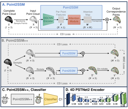
Figure 1: A. Point2SSM [16] architecture B. Point2SSM++ architecture C. Point2SSM++, Classifer architecture D. PSTNet [52] 4D encoder architecture.

As shown in Fig. 1.A, the Point2SSM model consists of two subnetworks: the encoder, which learns a feature representation of each input point and its neighbors, and the attention module, which estimates an attention map $\mathbf{W}$ from the features. DGCNN [37] is selected for the encoder architecture, enabling topological information to be learned via edge convolution. The encoder takes a point $\mathbf{x}_{n}\in{\mathbb{X}}$ and its $K$ nearest neighbors (with respect to Euclidean distance) as input and produces an $L$-dimensional feature representation ${\mathbf{f}}_{n}\in\mathbb{R}^{L}$ (corresponding to the $n$-th row in the learned feature matrix $\mathbf{F}$). By incorporating the spatial relation between points, the DGCNN encoder provides features that capture the local semantic characteristics of the shape. The attention module takes a feature vector ${\mathbf{f}}_{n}$ as input and outputs ${\mathbf{w}}_{n}\in\mathbb{R}^{M}$ (representing the $n$-th row in the weight map $\mathbf{W}$). The vector ${\mathbf{w}}_{n}$ captures the degree to which input point $n$ contributes to determining the positions of each of the $M$ output correspondence points (see Eq. 1). Point2SSM and its extension are permutation invariant because each row of the attention map is independently determined from a given point and its neighbors, i.e., permuting the input ${\mathbb{X}}$ identically permutes the rows of $\mathbf{W}$ providing the same ${\mathbb{Y}}$. The attention module utilizes self-attention to predict the attention map from the feature representation via self-feature augment (SFA) blocks originally introduced in [43]. The SFA block is a multihead, self-attention mechanism that draws on the core idea of transformers to optimally integrate the information from different point features.

III-B2 Loss

In Point2SSM, the attention map, $\mathbf{W}$, is learned in a self-supervised manner by encouraging ${\mathbb{Y}}$ to match the full point clouds ${\mathbb{S}}$. The Point2SSM loss is comprised of two terms - one that encourages ${\mathbb{Y}}$ to reconstruct ${\mathbb{S}}$ and one that regularizes ${\mathbb{Y}}$ across a minibatch, encouraging better correspondence.

Chamfer distance (CD) is used for the reconstruction loss term, as it quantifies the difference between the point clouds in a permutation-invariant way:

$$\mathrm{CD}({\mathbb{Y}},{\mathbb{S}})=\frac{1}{|{\mathbb{Y}}|}\sum_{{\mathbf{y}}\in{\mathbb{Y}}}\min_{{\mathbf{s}}\in{\mathbb{S}}}||{\mathbf{y}}-{\mathbf{s}}||_{2}^{2}+\frac{1}{|{\mathbb{S}}|}\sum_{{\mathbf{s}}\in{\mathbb{S}}}\min_{{\mathbf{y}}\in{\mathbb{Y}}}||{\mathbf{s}}-{\mathbf{y}}||_{2}^{2}$$ (2)

Other point cloud distance metrics have been proposed, such as Cauchy-Schwartz divergence [53] and variants of Earth Mover’s distance [54]. However, as supplementary experiments in Appendix A show, Chamfer Distance performs best on this task. Note that while Point2SSM is provided only with a subset of ${\mathbb{S}}$ as input, denoted ${\mathbb{X}}$, the CD loss is computed between ${\mathbb{Y}}$ and the full ${\mathbb{S}}$. In training, ${\mathbb{X}}$ is randomly sampled from ${\mathbb{S}}$ in each iteration, serving as an automatic form of data augmentation and leveraging the benefits of masked modeling. This approach improves model robustness as demonstrated by supplementary experiments in Appendix A.

A pairwise mapping error (ME) [15] provides a regularization term to improve correspondence. The ME between two output point clouds ${\mathbb{Y}}^{(1)}$ and ${\mathbb{Y}}^{(2)}$ is defined as:

$$\text{ME}({\mathbb{Y}}^{(1)},{\mathbb{Y}}^{(2)})=\frac{1}{M*R}\sum_{m=1}^{M}\sum_{r\in\mathcal{N}_{(1)}\left({\mathbf{y}}^{(1)}_{m}\right)}v^{(1)}_{mr}\left\|{\mathbf{y}}^{(2)}_{m}-{\mathbf{y}}^{(2)}_{r}\right\|_{2}^{2}$$ (3)

where $\mathcal{N}_{(1)}\left({\mathbf{y}}^{(1)}_{m}\right)$ are the $R$-indices of the $R$-nearest neighbors of point ${\mathbf{y}}^{(1)}_{m}$ in ${\mathbb{Y}}^{(1)}$ (in Euclidean distance). The term $v^{(1)}_{mr}=e^{-\left\|{\mathbf{y}}^{(1)}_{m}-{\mathbf{y}}^{(1)}_{r}\right\|_{2}^{2}}$ weights the loss elements according to the proximity of the neighbor points. The ME loss encourages point neighborhoods in ${\mathbb{Y}}^{(1)}$ to match those in ${\mathbb{Y}}^{(2)}$. Consistent point neighborhoods are an indication of accurate correspondence across shapes. ME is computed between all pairs of output in a minibatch of size $B$.

Given a batch of point cloud shape representations denoted $\mathcal{S}_{B}$ and predictions $\mathcal{Y}_{B}$, the Point2SSM loss is defined as:

$$\mathcal{L} {}_{\text{Point2SSM}}(\mathcal{S}_{B},\mathcal{Y}_{B})=\frac{1}{B}\sum_{i=1}^{B}\mathrm{CD}({\mathbb{Y}}^{(i)},{\mathbb{S}}^{(i)})+$$

$$\alpha\left(\frac{1}{(B-1)^{2}}\sum_{i=1}^{B}\sum_{j=1,j\neq i}^{B}\mathrm{ME}({\mathbb{Y}}^{(i)},{\mathbb{Y}}^{(j)})+\mathrm{ME}({\mathbb{Y}}^{(j)},{\mathbb{Y}}^{(i)})\right)$$

where $\alpha$ is a hyperparameter that controls the effect of the regularization [16]. In this work, $\alpha$ is set to 0.1 based on tuning using the validation set. Point2SSM accuracy is not particularly sensitive to the choice of $\alpha$ [16].

III-B3 Inductive Biases that Promote Learning Correspondence

Point2SSM was shown to provide output points in correspondence across the population, but it lacked a thorough argument to explain this behavior. This effect can be understood from the lens of information bottleneck (IB) theory, where a latent encoding is learned to capture the minimal sufficient statistics required of the input to predict the output [55]. The CD loss (Eq. 2) indirectly requires the features $\mathbf{F}$ to capture significant information from ${\mathbb{X}}$ relevant for accurately predicting ${\mathbb{Y}}$. The parameter $K$, determining the size of the neighborhood considered for each point, influences the degree of local versus global information captured in each feature encoding ${\mathbf{f}}_{n}$. Hence, the choice of $K$ controls the granularity of the information extracted for each point in the point cloud. This compression aligns with the IB principle’s aim to minimize the entropy between the input and latent encoding. The parameter $K$ must be optimally selected to capture enough local information without overfitting or including irrelevant information, as demonstrated by supplementary experiments in Appendix B. The attention module assigns weights to the feature vectors based on their relevance for generating ${\mathbb{Y}}$, effectively allowing the network to focus on the most informative aspects of $\mathbf{F}$ for predicting ${\mathbb{Y}}$. This process aligns with the IB principle’s aim to maximize the entropy between the latent encoding and output. In this manner, Point2SSM learns to discard redundant or noisy information in ${\mathbb{X}}$ that does not contribute to the accurate prediction of ${\mathbb{Y}}$, thereby enhancing the network’s ability to generalize and identify correspondences based on robust and distinctive features. At the same time, the attention module ensures that the retained information in $\mathbf{F}$ is maximally useful for the reconstruction task, which entails identifying and leveraging patterns (correspondences) that are consistent across different instances of the shape.

III-C Point2SSM++

This section details the proposed approach, Point2SSM++. Point2SSM++ improves output consistency by augmenting two different inputs ${\mathbb{X}}$ and $\widetilde{{\mathbb{X}}}$, of the same point cloud ${\mathbb{S}}$ as shown in Fig. 1.B. Point2SSM++ also allows for misaligned input and can be adapted for multi-anatomy and spatiotemporal scenarios, as explained in the following subsections.

III-C1 Allowing for Misaligned Input

Point2SSM assumes that input shapes are prealigned to remove the impact of translation, rotation, and scale in output predictions. Point2SSM++ removes this requirement, allowing for accurate predictions given input in any coordinate frame. This is partially accomplished by automatically normalizing input point clouds to be zero-centered with a uniform scale. Centering is performed by translating each point cloud center of mass to the origin and scaling is applied so that the maximum distance of any point to the origin is one. The inverse of these transforms is then applied to network output to provide predictions in the original coordinate system. Rotation generally cannot be automatically factored out as there is no notion of standard orientation. However, point clouds acquired from medical imaging data have an innate orientation resulting from the scanning process. Point2SSM++ capitalizes on this semantic orientation but accounts for small differences in patient pose via a consistency loss, as explained in the following section. In this manner, Point2SSM++ provides consistent predictions in the original input coordinate systems. In SSM analysis, correspondence points are mapped to a global coordinate system via generalized Procrustes [56] so that translation, rotation, and, optionally, scale are not captured as modes of variation. An experiment qualitatively demonstrating the efficacy of this approach for handling misaligned input is provided in Appendix C.

III-C2 Point2SSM++ Consistency Loss

Accurate SSM construction methods should provide consistent correspondence points given different samplings of the same input shape. As is illustrated in Fig. 1.B, Point2SSM++ directly encourages this quality by quantifying the consistency in predictions resulting from two different random subsamples, ${\mathbb{X}}$ and $\widetilde{{\mathbb{X}}}$, of the same point cloud ${\mathbb{S}}$. Additionally, accurate correspondence points should be unaffected by pose, i.e., rotationally equivariant. To account for pose, Point2SSM++ samples random $x$, $y$, and $z$ rotations within $\pm 15$ degrees and applies them to input $\widetilde{{\mathbb{X}}}$. The inverse rotation is then applied to the resulting prediction to get $\widetilde{{\mathbb{Y}}}$. The consistency between the resulting predictions, ${\mathbb{Y}}$ and $\widetilde{{\mathbb{Y}}}$ is then quantified via mean square error (MSE). Note rotation augmentation could be added to ${\mathbb{X}}$ in addition to $\widetilde{{\mathbb{X}}}$; however, we elect to preserve the original orientation since it retains semantic consistency in clinical scenarios.

The Point2SSM++ loss is formulated as the Point2SSM loss (Eq. LABEL:eq:loss) computed on both ${\mathbb{Y}}$ and $\widetilde{{\mathbb{Y}}}$, as well as this consistency term. Thus, given a batch of point clouds $\mathcal{S}_{B}$ and predicted output $\mathcal{Y}_{B}$, the Point2SSM++ loss is defined as:

$$\mathcal{L}_{\text{Point2SSM++}}(\mathcal{S}_{B},\mathcal{Y}_{B}) =\mathcal{L}_{\text{Point2SSM}}(\mathcal{Y}_{B},\mathcal{S}_{B})$$

$$+\mathcal{L}_{\text{Point2SSM}}(\widetilde{\mathcal{Y}}_{B},\mathcal{S}_{B})$$

$$+c*\frac{1}{B}\sum_{i=1}^{B}\mathrm{MSE}({\mathbb{Y}}^{(i)},{\mathbb{Y}}^{(i)*})$$ (5)

where $c$ is a scalar hyperparameter, determining the weight of the consistency term. In this work, $c$ is set to 1 in all experiments based on tuning using the validation set. This loss encourages surface sampling invariance and rotation equivariance, making Point2SSM robust to differences in pose and improving correspondence accuracy.

III-C3 Point2SSM++ Multi-Anatomy Training

Training Point2SSM [16] on multiple anatomies was shown to provide similar accuracy to training individual single-anatomy models. Point2SSM++ can similarly be trained on multiple anatomies, which enables leveraging shared shape information to inform correspondence predictions for each anatomy, improving accuracy when training data for a given anatomy type is limited. The training and inference processes are identical to the single anatomy case. In analysis, Procrustes alignment and evaluation metric calculation are performed per anatomy type to capture anatomy-specific statistics and allow for comparing results with the single anatomy model.

A concern in multi-anatomy training is the potential loss of anatomy-specific features. To mitigate this effect, we propose augmenting the Point2SSM++ model with an auxiliary anatomy classifier, depicted in Fig. 1.C. The MLP classification module is trained to predict the anatomy from ${\mathbb{Y}}$, and a negative log-likelihood classification loss term is added, encouraging the model to generate multi-anatomy SSM that preserves anatomy-specific morphological characteristics, facilitating clearer differentiation among different anatomies to be encoded in the output correspondence points.

III-C4 Spatiotemporal (4D) Point2SSM++

Many clinical research studies require assessing dynamic or longitudinal cases of 4D data or sequences of shapes over time. In order to extend the Point2SSM++ method to 4D data, we propose replacing the 3D DGCNN encoder with a state-of-the-art point cloud sequence convolutional network: the hierarchical Point Spatio-Temporal net (PSTnet2) [52] ( Fig. 1.D). In the Point2SSM++ model with PSTNet2 encoder, denoted 4D PSTNet2 Point2SSM++, the loss and attention module remain the same and are applied cross-sectionally, but the PSTNet2 encoder enables learning 4D point cloud features.

III-D Evaluation Metrics

The quality of correspondence-based SSM relies on two key factors: how well points are constrained to and capture the shape surfaces and how well the population-level statistics are captured through correspondence. These aspects are not mutually dependent; as a strong correspondence model might inadequately sample underlying surfaces, and vice versa. We utilize nine complementary metrics for thorough evaluation:

III-D1 Surface Sampling

• Chamfer distance (CD): A small CD (Eq. 2) indicates the output points accurately capture the complete shape.

• Point-to-surface distance (P2S): P2S quantifies the distance of the output points to a complete surface shape representation (i.e., mesh). Low P2S indicates that predicted points are well constrained to the shape surface.

III-D2 Consistency

• Sampling invariance (Samp. MSE): Accurate predictions should be invariant to different input samplings of the same shape. This metric is evaluated as the mean square error (MSE) between predictions made from two different random subsamples of the same test point cloud.

• Rotation equivariance (Rot. MSE): Accurate predictions should be equivariant to differences in pose or rotation. This metric is evaluated as the mean square error (MSE) between aligned predictions made from two different random rotations of the same test input.

III-D3 Correspondence

• Mapping error (ME): The ME (Eq. 3) quantifies how consistent output point neighborhoods are across the population. A lower ME indicates consistent neighborhoods, implying better correspondence.

• Warp-based reconstruction surface-to-surface distance (Warp S2S): Accurate correspondence points can serve as control points for surface mesh warping. Given two sets of correspondence points ${\mathbb{Y}}^{(1)}$ and ${\mathbb{Y}}^{(2)}$ and corresponding surface mesh $\mathbf{M}^{(1)}$, a reconstructed surface mesh $\widehat{\mathbf{M}}^{(1)}$ can be obtained by applying the warp between ${\mathbb{Y}}^{(2)}$ and ${\mathbb{Y}}^{(1)}$ to $\mathbf{M}^{(2)}$. A smaller surface-to-surface distance between $\mathbf{M}^{(1)}$ and $\widehat{\mathbf{M}}^{(1)}$ indicates better correspondence between the control points.

III-D4 SSM Metrics

Principal component analysis (PCA) is used in SSM analysis to quantify the modes of variation in the population and assess how well population-level statistics are captured [57]. There are three metrics to this end:

• Compactness (Comp.): Accurate correspondence leads to a more compact SSM, meaning the training data distribution is represented using the minimum number of parameters. When there is strong correspondence, a large proportion of explained population variance is captured in fewer PCA modes. Thus, a larger area under the cumulative variance plot indicates better correspondence.

• Generalization (Gen. CD): Accurate SSM should generalize well from training examples to unseen examples. The generalization metric quantifies the CD between the estimated correspondences from test point clouds and their reconstructions from the training SSM-based PCA embeddings with various numbers of components. A smaller CD indicates that the SSM generalizes better.

• Specificity (Spec. CD): Specifity measures whether the SSM generates valid instances of the shape class. It is computed as the average CD between training examples and generated samples from the training SSM-based PCA embeddings with various numbers of components. A smaller CD indicates the SSM is more specific.

IV Experiments

In all experiments, unless otherwise specified: $|{\mathbb{S}}|\approx 5000$, $|{\mathbb{X}}|=N=1024$, $|{\mathbb{Y}}|=M=1024$, $K=26$, $L=128$, and batch size $B=8$ or $B=4$ in the case of Point2SSM++. These values were selected to be consistent with existing work. Point2SSM has been shown to be robust to the choice of $N$, $M$, $B$ [16], and $K$ (Appendix B). Adam optimization with a constant learning rate of 0.0001 is used on a 4x TITAN V GPU to train models. Model training is run until convergence (i.e., when CD on the validation set has not improved in 100 epochs). All evaluation utilizes the models resulting from the epoch with the best validation CD.

IV-A Nonlinear Variation Proof of Concept

Point cloud deep learning-based SSM generation techniques, such as Point2SSM++, are data-driven and do not rely on any limiting assumptions about the underlying data distribution. Traditional SSM generation methods require assumptions to define optimization objectives or require a template or atlas. PSM [18] utilizes a Gaussian entropy-based optimization objective that imposes a linearity assumption, biasing the population variation captured.

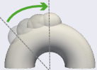
Figure 2: Mode of variation in half torus bump shapes.

To illustrate this difference, we utilize a synthetic dataset with known nonlinear shape variation, comprising half torus shapes with a protruding bump. The shapes are identical across the cohort with the exception of the position of the bump, which varies along a curve, as illustrated in Figure 2. Thus, this dataset exhibits a singular, nonlinear mode of variation.

Fig. 3 provides example correspondence points and the primary and secondary modes of variation resulting from PSM and Point2SSM++. A single point on the bump is highlighted across three test predictions, with color denoting distance to the point. In the Point2SSM++ model, this point consistently stays on the bump across the population as expected, whereas the PSM model fails to maintain this correspondence. This result is further illustrated by the modes of variation, where Point2SSM++ correctly finds the singular true nonlinear mode, whereas PSM fabricates two linear modes to account for the variation. Furthermore, the mean shape resulting from our approach resembles a valid instance of the shape class, whereas the mean shape from PSM does not.

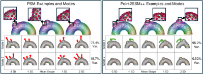
Figure 3: Results on the nonlinear half torus bump dataset from PSM and Point2SSM++. The three example test predictions (top) and resulting primary and secondary modes of variation (bottom) demonstrate that Point2SSM++ correctly captures nonlinear variation, whereas PSM fails to do so.

IV-B Single Anatomy Experiments

We utilize challenging single anatomy datasets to comprehensively analyze the performance of Point2SSM++ compared to PSM and point cloud deep learning-based methods. The following subsections outline the datasets and comparison models and provide results and downstream task analysis.

IV-B1 Datasets

We employ publicly available segmentation datasets comprising six distinct anatomies with varying cohort sizes. These datasets feature complete mesh shape representations, facilitating comparison with the traditional PSM method. The unordered mesh vertices serve as the ground truth complete point clouds. All datasets undergo random partitioning into training, validation, and testing sets using an $80\%/10\%/10\%$ split. Each dataset is described as follows:

• Spleen (40 shapes)[58]: The spleen organ dataset provides a limited data scenario with challenging shapes that vary greatly in size and curvature.

• Pancreas (272 shapes)[58]: The pancreas dataset comprises of pancreas organs with tumors of varying sizes from cancer patients, providing difficult patient-specific shape variability.

• Liver (834 shapes) [59]: The liver dataset provides a organ datasets with nonlinear shape variation.

• Femur (56 shapes): The femur dataset contains proximal femur bones clipped under the lesser trochanter to focus on the femoral head. Nine of the femurs have the cam-FAI pathology characterized by an abnormal bone growth lesion that causes hip osteoarthritis [2].

• L4 Vert. (160 shapes)[60]: This dataset contains fourth lumbar (L4) vertebrae bones, with complex topology.

• Cranium (400 shapes)[4]: This dataset contains 3D head models constructed from surface scans of craniosynostosis patients. There are four balanced classes within this dataset: control and three pathological suture fusion classes (coronal, metopic, and sagittal).

IV-B2 Comparison Models

We compare Point2SSM and Point2SSM++ with the traditional PSM model, as well as SOTA point cloud deep learning based models. Each method is described as follows:

• PSM [22] is the SOTA optimization-based method that requires a complete surface shape representation. We use its open-source implementation in ShapeWorks[22]. It is included to provide a reference point for the SSM metrics.

• DG-AE [37] is the autoencoder formulated by [61] with the same DGCNN [37] encoder as Point2SSM.

• ISR [14] is the method proposed for learning intrinsic structural representation (ISR) points via PointNet++ [62] encoder and an MLP point integration module.

• DPC [15] is the pairwise deep point correspondence (DPC) model that reorders a source point cloud to match a target point cloud via latent similarity. In inference, we set the target as the point cloud with the minimum CD to all others to acquire population-level correspondence.

• SC3K [51] is the Self-supervised and Coherent 3D Keypoints (SC3K) estimation method proposed in concurrence with Point2SSM. This method detects sparse keypoints from point clouds that are noisy, down-sampled, and arbitrarily rotated.

• SC3K* [51] denotes the SC3K model with our Point2SSM++ loss (Eq. 5). The original SC3K loss was proposed for sparse output points ($\mathbf{M}\approx 10$) and was shown to fail given denser output ($\mathbf{M}>50$) [51]. Thus, we include SC3K* to compare the SC3K and Point2SSM++ architectures alone.

• Point2SSM [16] is the model described in section III-B.

• Point2SSM++ is the proposed model described in section III-C.

IV-B3 Results

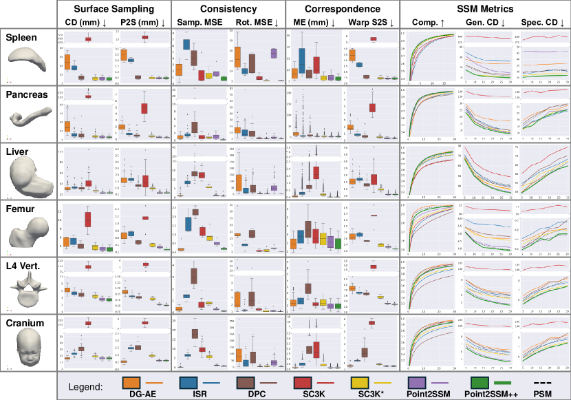
Figure 4: Single anatomy experiment results. Boxplots show the error distribution across test sets for each model in mm. Compactness plots show the cumulative variance ratio over the number of PCA modes. Generalization and specificity plots show the CD over the number of PCA modes. A maximum of 30 modes is displayed which captures at least $99\%$ of the total variation for all datasets. Lower values are better for all metrics except PCA compactness.

Fig. 4 summarizes the results across metrics (section III-D), datasets (section IV-B1), and models (section IV-B2). Point2SSM++ provides the best overall accuracy, outperforming the other point cloud deep learning based methods in terms of surface sampling, consistency, and correspondence. Additionally, Point2SSM++ matches the traditional PSM model performance on SSM metrics, achieving similar or better compactness and better generalization and specificity while significantly relaxing the input shape requirement.

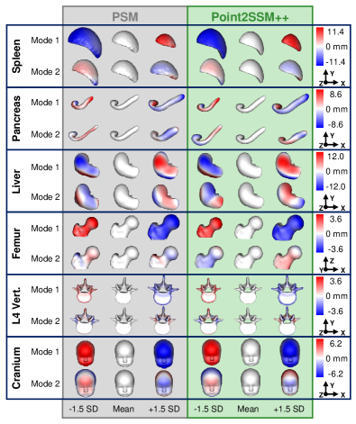
Figure 5: Primary and secondary modes of population variation captured by the PSM (gray) and Point2SSM++ (green) methods across each dataset. The mean and shapes at $\pm 1.5$ standard deviation are shown with color denoting the distance to the mean. Blue indicates the surface is outside the mean, and red indicates the surface is inside the mean. Separate color scales and orientation markers are provided for each dataset.

Fig. 5 shows the primary and secondary modes of variation captured by the PSM and Point2SSM++ methods for each of the datasets. A similar visualization is provided for all comparison models in Appendix D. The mean and shapes at $\pm 1.5$ standard deviation are displayed as meshes, generated via mesh warping using the output correspondence points as control points. Point2SSM++ provides similar, if not more, smooth and interpretable mean shapes and modes of variation as PSM. The mean shapes resulting from PSM on datasets with a large amount of linearity (i.e., spleen and pancreas) have some artifacts indicating some miscorreposondence impacting the mesh warping. The Point2SSM++ mean shapes do not have this issue. In most cases, the primary modes found by the two methods are similar, with size often captured as the first mode. This result suggests that Point2SSM++ is correctly capturing the population-level statistics of each shape cohort.

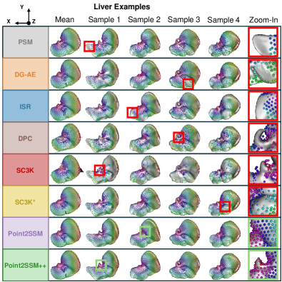
Figure 6: The mean correspondence points and four example predictions from the test set are provided from each approach on the liver dataset. The mean mesh is constructed via mesh warping. Sample correspondence point predictions are overlaid over ground truth meshes. Color denotes correspondence. An illustrative zoom-in box is provided for each model.

Fig. 6 provides qualitative results on the liver dataset. The mean correspondence points from each model are displayed, as well as four example predictions from the test set. The mean correspondence points should represent a plausible liver. Mean meshes are reconstructed via correspondence-based mesh warping, thus mesh artifacts suggest miscorrespondence. Point2SSM++ provides a plausible mean shape with a smooth mesh, whereas the mean meshes resulting from other methods (such as DPC and SC3K) have artifacts. All methods establish reasonable correspondence, as can be seen by the color of the points in Fig. 6. However, not every method provides good surface sampling, as can be seen in the red zoomed-in boxes on the right, which highlight predicted points that do not lie on the true surface. Even in the case of the traditional PSM method, where points are directly constrained to the surface, the points do not cover the entire shape due to the high variability of the liver shape. Point2SSM++ provides the best correspondence with uniformly spread points, constrained to the surface in semantically consistent locations across the samples.

IV-B4 Downstream Task Analysis

The femur and cranium datasets have subgroups, enabling downstream clinical task analysis. The femur dataset contains 47 healthy/control subjects and 9 with CAM pathology, characterized by an abnormal bone growth lesion on the femoral neck that limits motion and is associated with hip osteoarthritis [2]. The Point2SSM++ model captures this difference similarly to the traditional PSM method, as seen by the colormap distance between the means in Fig. 7. This experiment serves as an example of how Point2SSM++ can be used to characterize pathology.

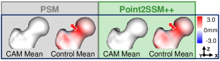
Figure 7: Femur group differences from PSM and Point2SSM++. CAM pathology and control group mean shapes are displayed. Color denotes the distance from the control mean to the CAM mean. The pathology is correctly captured as a widening of the femoral neck.

The cranium dataset contains control samples and three categories of craniosynostosis, a disorder in which one or more of the sutures between the bones of infants’ cranial sutures fuse prematurely. In Fig. 8, we utilize the Point2SSM++ output to compare the mean shape of each of these subgroups to the control group. Each of the subgroups is correctly characterized, with coronal synostosis manifesting as a flattening of the forehead, metopic as a triangulation of the forehead, and sagittal as a narrowing of the skull.

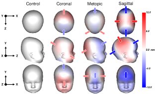
Figure 8: Cranio group differences. The mean shape of each group resulting from Point2SSM++ predicted SSM is shown from multiple views. Color denotes the distance of the shapes to the control mean shape. Arrow annotations are provided to show the general trends.

SSM on the cranium dataset could be useful in classifying new shapes as normal cases or as one of the three types of craniosynostosis. We trained a classifier on SSM predictions from each construction technique to explore their effectiveness for classification. In particular, first, correspondences were obtained on training and testing samples using each model. Then, we trained a support vector classification model with RBF kernels on the training correspondences and evaluated the classification accuracy on test correspondences. We utilized five fold cross-validation to repeat this experiment five times with different train/test splits to ensure fair analysis. Note the classes are balanced in this dataset and in all splits. The results are summarized in Table I. All SSMs correctly classified at least $93\%$ of the cases, but Point2SSM and Point2SSM++ provided the best accuracy at $98.2\%$ correct. These results further indicate Point2SSM++ provides SSM that correctly captures the morphology indicative of the subtypes of craniosynostosis.

TABLE I: Craniosynostosis classification accuracy: Mean values of ratio of correctly classified instances and class F1 scores are with standard deviation from five fold cross-validation.

		Class F1 Score $\uparrow$
Model	Accuracy $\uparrow$	Control	Coronal	Metopic	Sagittal
PSM	0.965$\pm$0.015	0.943$\pm$0.032	0.963$\pm$0.032	0.985$\pm$0.012	0.969$\pm$0.020
DG-AE	0.977$\pm$0.005	0.975$\pm$0.017	0.995$\pm$0.010	0.980$\pm$0.019	0.959$\pm$0.013
ISR	0.930$\pm$0.026	0.902$\pm$0.039	0.950$\pm$0.035	0.934$\pm$0.041	0.933$\pm$0.037
DPC	0.953$\pm$0.028	0.941$\pm$0.025	0.964$\pm$0.036	0.937$\pm$0.028	0.969$\pm$0.039
SC3K	0.970$\pm$0.023	0.968$\pm$0.052	0.980$\pm$0.019	0.960$\pm$0.019	0.970$\pm$0.019
SC3K*	0.970$\pm$0.010	0.960$\pm$0.021	0.980$\pm$0.010	0.970$\pm$0.019	0.969$\pm$0.020
Point2SSM	0.982$\pm$0.006	0.985$\pm$0.021	0.985$\pm$0.012	0.985$\pm$0.012	0.974$\pm$0.017
Point2SSM++	0.982$\pm$0.006	0.985$\pm$0.012	0.985$\pm$0.012	0.990$\pm$0.012	0.969$\pm$0.020

IV-C Multi-Anatomy Experiments

We utilize three models in multi-anatomy experiments:

• Single Anatomy Point2SSM++ denotes the model trained and tested on only a single anatomy, as was done in section IV-B.

• Multi-Anatomy Point2SSM++ denotes the model trained on multiple anatomies.

• Multi-Anatomy Point2SSM++, Classifier denotes the multi-anatomy Point2SSM++ model with an auxiliary classifier as explained in section III-C3.

The following sections detail multi-anatomy experiment results on two different datasets.

IV-C1 Multi-Organ Experiment

The multi-organ dataset is comprised of three anatomy types: the spleen, pancreas, and liver datasets described in section IV-B1. We randomly select a subset of 32 training shapes for each organ, resulting in a total training set of 96. The single anatomy Point2SSM++ models are individually trained on each subset of 32 shapes. This experiment provides an example of multi-anatomy training with large differences between anatomy types.

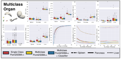
Figure 9: Multi-organ results. Metrics are reported for the three models across the three organs. Different line types in the PCA plots differentiate organs.

The results are compiled in Figure 9. The multi-anatomy Point2SSM++ models achieve the best performance, demonstrating that by increasing the training set size via multi-anatomy training, the model is made more robust. These results suggest that an anatomy-agnostic multi-anatomy Point2SSM++ could be trained on a wide variety of shapes to provide a foundational SSM model.

IV-C2 Vertebrae Experiment

The vertebrae dataset includes 24 vertebrae bones from the TotalSegmentator dataset [63]. This includes cervical (C1-C7), thoracic (T1-T12), and lumbar spine (L1-L5). We randomly select 30 training, 30 validation, and 100 test shapes for each bone to create this dataset. The bones have shared shape properties but vary significantly between classes, as can be seen in Fig. 10. Additionally, the bone segmentations in this dataset are binary mask volumes with varying resolution and often large $z$-spacing, many of which have artifacts like holes and islands. Thus, acquiring complete surface meshes is difficult. We utilize marching cubes to extract point clouds from the binary volumes for Point2SSM++ input. This experiment reinforces the versatility of Point2SSM++, as it can be used given imperfect input.

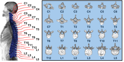
Figure 10: Example of the 24 vertebrae bones from side and top view.

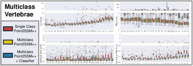
Figure 11: Multi-anatomy vertebrae results. Metrics are reported for the three models across the 24 vertebrae.

Evaluation metrics for each of the 24 vertebrae are provided in Fig. 11. Note the P2S and Warp P2P metrics are excluded here due to the lack of ground truth surface meshes. The multi-anatomy models perform similarly or better than the single anatomy model across all vertebrae. SSM metric plots would be difficult to interpret with all bones, and thus summary values are reported in Table II. Here, compactness is quantified as the number of modes required to capture $95\%$ of the variation, and generalization and specificity are reported with that number of modes. The single anatomy and multi-anatomy models provide similar PCA statistics. Fig. 12 shows that the multi-anatomy Point2SSM++ model with the auxiliary classifier model provides correspondence across different vertebrae. This visualization highlights the utility of the approach, as it can be used to quantify and characterize shape differences not only within each anatomy but also across anatomy types.

TABLE II: Multiclass Vertebrae SSM Metrics

Vert.	Compactness $\downarrow$			Generalization CD (mm) $\downarrow$			Specificity CD (mm) $\downarrow$
	Single	Multi	Multi + Classifier	Single	Multi	Multi + Classifier	Single	Multi	Multi + Classifier
C1	18	17	17	3.12	3.09	3.1	3.38	3.34	3.34
C2	14	14	14	2.76	2.75	2.75	3.04	3.04	3.09
C3	18	17	18	2.68	2.64	2.64	3.13	3.15	3.15
C4	18	17	17	2.9	2.78	2.75	3.5	3.44	3.47
C5	15	14	14	2.92	2.87	2.86	3.83	3.96	3.87
C6	13	13	13	3.32	3.31	3.28	3.52	3.59	3.54
C7	8	8	8	3.7	3.73	3.7	3.4	3.59	3.5
T1	15	13	13	3.7	3.6	3.64	3.67	3.63	3.6
T2	12	11	12	2.97	3.03	3.01	3.62	3.58	3.66
T3	13	13	13	3.0	3.03	2.97	3.23	3.32	3.31
T4	10	9	10	3.37	3.5	3.43	3.55	3.55	3.56
T5	13	12	13	3.63	3.54	3.53	3.8	3.81	3.84
T6	13	11	11	4.12	4.14	4.2	3.82	3.77	3.8
T7	10	10	11	6.13	6.38	6.33	3.94	4.04	4.07
T8	9	8	9	4.6	4.75	4.62	3.91	3.92	3.98
T9	12	11	11	4.33	4.18	4.22	4.66	4.6	4.6
T10	14	13	14	5.17	4.93	5.0	4.53	4.52	4.5
T11	17	15	16	4.54	4.48	4.44	4.74	4.82	4.74
T12	18	16	16	5.4	5.39	5.47	4.67	4.74	4.7
L1	17	16	16	5.61	5.48	5.44	5.17	5.16	5.23
L2	16	15	16	5.68	5.47	5.5	5.59	5.44	5.6
L3	11	10	10	6.91	6.96	7.01	7.01	7.09	6.97
L4	13	13	13	7.73	7.64	7.69	6.72	6.72	6.69
L5	15	15	14	7.18	7.19	7.21	6.59	6.66	6.5
Avg.	13.83	12.96	13.29	4.39	4.37	4.37	4.29	4.31	4.30

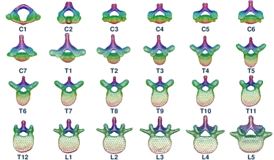
Figure 12: The mean predictions from the multi-anatomy Point2SSM++, Classifier model for each vertebrae. Color denotes correspondence.

TABLE III: Multiclass Vertebrae Classification Accuracy

Model	Overall Acurracy	Individual Vertebrae F1 Scores
		C1	C2	C3	C4	C5	C6	C7	T1	T2	T3	T4	T5	T6	T7	T8	T9	T10	T11	T12	L1	L2	L3	L4	L5
Multi	0.6533	1.00	1.00	0.60	0.37	0.24	0.73	0.86	0.91	0.78	0.54	0.55	0.43	0.45	0.38	0.41	0.55	0.64	0.84	0.89	0.59	0.45	0.63	0.78	0.93
Multi+Class.	0.6825	1.00	1.00	0.62	0.42	0.28	0.80	0.86	0.92	0.79	0.61	0.63	0.50	0.48	0.45	0.36	0.60	0.68	0.82	0.88	0.61	0.46	0.67	0.81	0.94

The motivation behind including an auxiliary classifier is to promote learning anatomy-specific features. Thus, distinguishing between anatomy types in the output correspondence points should be easier. To evaluate this, we trained a classifier on the predictions made by the multi-anatomy Point2SSM++ with and without the auxiliary classifier. In particular, we fit a K-nearest neighbors classifier (with 10 neighbors) to the predicted training correspondence points and evaluate the accuracy of the predicted test correspondence points. The results are provided in Table III. The multi-anatomy model alone achieved an accuracy of $65.33\%$ whereas the multi-anatomy model with the auxiliary classifier achieved an accuracy of $68.25\%$. This difference suggests that while the models achieve similar performance on the metrics reported in Fig. 11 and Table II, the model with the auxiliary classifier does better in capturing anatomy-specific features.

IV-D Spatiotemporal (4D) Experiments

Next, we evaluate the ability to adapt Point2SSM++ to the case spatiotemporal/4D SSM where we have sequences of shape from a subject over time for dynamic or longitudinal clinical studies. The models evaluated on the task of spatiotemporal anatomical SSM are outlined as follows:

• Spatiotemporal PSM [26] denotes the 4D extension of the optimization-based PSM method. This approach injects the underlying time dependency into correspondence optimization via a regularized principal component polynomial regression across time. Like PSM, it requires a complete surface shape representation but is included to provide context for the SSM metrics.

• 3D Point2SSM++ denotes the proposed Point2SSM++ approach applied cross-sectionally to 4D data, ignoring the time dependency. This baseline is included to highlight the importance of modeling the time dependency.

• 4D PSTNet2 Point2SSM++ denotes the Point2SSM++ method where the 3D DGCNN encoder is replaced by the hierarchical Point Spatio-Temporal net (PSTnet2) [52], as explained in section III-C4.

IV-D1 4D Ellipsoid Experiment

We utilize a synthetic 4D ellipsoid dataset with known shape dynamics as proof of concept. These ellipsoids are parameterized by a subject-specific $x$-diameter (randomly selected from a Gaussian distribution), a time-dependent $y$-diameter, and a fixed population consistent $z$-diameter value, as summarized in Fig. 13.

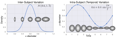
Figure 13: The functions defining the diameters of the synthetic 4D ellipsoid dataset are shown with example shapes. The $x$-diameter provides inter-subject variation, and the $y$-diameter provides intra-subject variation across time.

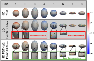
Figure 14: Mean correspondence points resulting from each model are shown over reconstructed meshes. Point color denotes correspondence. Mesh color denotes the distance to the next time point mean.

Fig. 14 shows the predicted mean correspondence points across time resulting from each of the models. All three methods correctly find the significant modes of variation, meaning two significant modes across subjects and time ($x$ and $y$ diameter), one significant mode across subjects within each time point ($x$-diameter), and one significant mode across time within each subject’s sequence ($y$-diameter). However, as can be seen in Fig. 14, the 4D PSTNet2 Point2SSM++ model provides better correspondence than the 3D Point2SSM++ method applied cross-sectionally. This proof of concept experiment demonstrates the benefit of using a 4D encoder in Point2SSM++ with spatiotemporal datasets.

IV-D2 4D Left Atrium Experiment

Next, we analyze the accuracy of the 4D PSTNet2 Point2SSM++ method compared to the traditional approach, 4D PSM, on a real spatiotemporal anatomical dataset: the left atrium of the heart. This dataset includes 3D late gadolinium enhancement (LGE) and stacked cine cardiovascular magnetic resonance (CMR) scans from 28 patients with atrial fibrillation, gathered prior to radiofrequency ablation procedures. Each cine scan consisted of 25 time points covering a single cardiac cycle (between R-wave peaks), with temporal normalization during acquisition to encompass one heartbeat per patient. The 3D LGE images were segmented manually by a cardiac imaging specialist and aligned with the nearest cine time point based on CMR trigger time. This segmentation was then propagated to all time points using pairwise deformable registrations, resulting in a complete 3D segmentation for each time point [64].

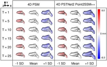
Figure 15: The primary mode of variation resulting from the 4D PSM method and 4D PSTNet2 Point2SSM++ on the left atrium at various time points is shown from the top view. Color denotes the distance to the mean shape.

Fig. 15 shows the mean shape and primary mode of variation captured across time by 4D PSM and 4D PSTNet2 Point2SSM++. The mean shape and variation are similar; however, the 4D PSTNet2 Point2SSM++ mesh constructions have fewer artifacts in the pulmonary veins and left atrium appendage. This improvement indicates that the 4D PSTNet2 Point2SSM++ provides better correspondence.

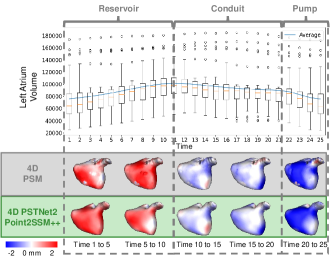
Figure 16: The three left atrium function intervals are shown: reservoir, conduit, and pump. The top plot displays box plots of the left atrium volume across time. At the bottom the mean shapes from 4D PSM and 4D PSTNet2 Point2SSM++ are shown from the anterior view at a subset of time points. Heat maps show the change in shape to the next displayed time point mean shape (red denotes expansions and blue contraction).

The dynamics of the left atrium during a heartbeat are characterized by three steps: reservoir or filling (where the volume increases), conduit or passive emptying (where volume decreases slowly in a decelerating manner), and pump or active emptying (where volume decreases quickly). Fig. 16 shows that both methods correctly characterize this temporal dependency, as the mean shape dynamics correctly match the mean volume over time. However, as can be seen by the mean colormaps Fig. 16, 4D PSTNet2 Point2SSM++ provides a smoother characterization of the dynamics, indicating better correspondence. These results demonstrate that Point2SSM++ can easily be adapted to accurately capture both spatial and temporal variation in anatomical cohorts, enabling longitudinal and dynamic clinical studies.

V Conclusion

In this paper, we introduced Point2SSM++, a principled, self-supervised approach for constructing correspondence-based anatomical SSM directly from point clouds. Through extensive evaluation, we demonstrated Point2SSM++ outperforms existing deep learning-based methods while eliminating the need for preprocessing steps such as point cloud alignment. Moreover, our results indicate that Point2SSM++ matches or surpasses the performance of the optimization-based PSM method, while alleviating the associated burdens, including stringent input shape requirements, susceptibility to bias/assumptions, and prolonged inference processes. Additionally, our experiments involving multiclass and 4D spatiotemporal analyses showcase the versatility of Point2SSM++ across various clinical tasks. Potential avenues for future research include exploring probabilistic extensions of Point2SSM++ to provide estimations of uncertainty or model confidence, ensuring the reliability of predictions in clinical settings. As Point2SSM [16] has demonstrated robustness to imperfect input such as noisy, sparse, and partial point clouds, future investigations could also focus on directly enhancing this robustness in Point2SSM++.

Overall, Point2SSM++ significantly streamlines SSM construction and inference by removing all manual and automatic preprocessing steps and reducing computational overhead and time requirements. This improvement paves the way for SSM to become a widely accessible onsite clinical tool. Furthermore, Point2SSM++ expands the potential applications of SSM, enabling its use in scenarios where complete and clean shape representations are unavailable, as well as facilitating specific clinical research endeavors such as multiclass and longitudinal/dynamic studies. By enhancing the accessibility and versatility of SSM, Point2SSM++ has the potential to advance clinical knowledge and improve patient care.

Jadie Adams is a computing PhD candidate at the Kahlert School of Computing and the Scientific Computing and Imaging Institute at the University of Utah in the Image Analysis track. She received her B.S. in Mathematics from Westminster College in 2018. Her research interests include deep learning, computer vision, and statistical shape modeling.

Shireen Elhabian is a faculty member at the Kahlert School of Computing and the Scientific Computing and Imaging Institute at the University of Utah. Her research interests lie in developing advanced computer vision algorithms to improve diagnostic accuracy, with a specific focus on using deep learning and probabilistic modeling techniques to analyze medical images such as MRIs, CT scans, and histopathology images. She has published over 100 peer-reviewed publications in prestigious journals and conferences, including IEEE-TMI, MedIA, ICLR, CVPR, ICCV, MICCAI, IPMI, AAAI. Her contributions to developing AI-driven computational tools for image and shape analysis have attracted significant funding from federal agencies (NIH and NSF) and industrial contracts.

Appendix A Point Cloud Distance Metrics

A number of permutation-invariant distance metrics have been proposed for point cloud evaluation. Chamfer distance (CD) (Eq. 2) is a popular choice because it does not require the point clouds to have the same number of points. Earth Mover’s Distance (EMD) has been shown to outperform CD on learning representation tasks, but requires point clouds to have equal size and has significantly higher computational cost. Sliced Wasserstein distance (SWD) [54] is a more computationally efficient metric (based on projecting the points in point clouds onto a line) and has been shown to match EMD performance. Alternatively, Cauchy-Schwartz (CS) divergence, which calculates the divergence between two probability distributions, has been utilized [53]. By representing point clouds as probability density functions and seeking to minimize divergence between them, this metric is more robust to outliers. However, it is also symmetric and requires the point clouds to be the same size.

To empirically justify our choice of CD for the distance metric, we compare against SWD and CS across three datasets: spleen, pancreas, and L4 vertebrae. The loss was computed between ${\mathbb{S}}$ and ${\mathbb{Y}}$ for each distance metric. As SWD and CS require point clouds to be the same size, a downsampled version of ${\mathbb{S}}$ is created via furthest point sampling (FPS). For a fair comparison, we also compute CD using this downsampled version of $\mathbb{S}$, this metric is denoted FPS CD. The results are provided in Fig. 17. The CD loss performs best across metrics, supporting our choice in the Point2SSM loss and reinforcing the robustness provided by requiring the predicted points to match a more dense point cloud.

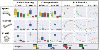
Figure 17: Results with different loss distance metrics are reported across three datasets. Boxplots show the error distribution across test sets for each model in mm. Compactness plots show the cumulative variance ratio over the number of PCA modes. Generalization and specificity plots show the CD over the number of PCA modes.

Appendix B Correspondence Ablation Experiment

The choice of $K$, or how many neighbors are used in graph construction for the DGCNN encoder, impacts the expressivity of the network. Here, we demonstrate this effect experimentally by training with different values of $K$, keeping $L$ fixed at 16 to limit the capacity of the feature representation. We perform this experiment using two loss functions: the self-supervised term used in Point2SSM $CD({\mathbb{S}},sY)$, and an input reconstruction loss $CD({\mathbb{X}},{\mathbb{Y}})$. The results are provided in Fig. 18. With $\mathrm{CD}({\mathbb{X}},{\mathbb{Y}})$ loss, the best results are achieved with $k$ values between 8 and 64. With too few neighbors or too many, performance on variance metrics suffers. For example, with $K=1$ the CD is good, but compactness is poor. Whereas with $K=256$, CD is poor. While the reconstruction loss, $CD({\mathbb{X}},{\mathbb{Y}})$ is sensitive to the choice of $K$, the self-supervised loss $CD({\mathbb{S}},{\mathbb{Y}})$ is robust to the choice of $K$.

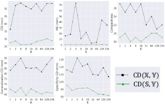
Figure 18: Impact of $K$ hyperparameter values with self supervised loss $CD({\mathbb{S}},{\mathbb{Y}})$ and reconstruction loss $CD({\mathbb{X}},{\mathbb{Y}})$.

Appendix C Alignment Comparison

Point2SSM assumed input point clouds are prealigned, whereas Point2SSM++ allows for misaligned input. To demonstrate this ability, we trained both on the same prealigned pancreas and spleen data. We then tested both models on three versions of the test datasets:

1. Prealigned - test data aligned to match the prealigned training data

2. Original - test data in the original coordinate system it was acquired from

3. Misaligned - test data with additional added misalignment in the form of random translations and rotations.

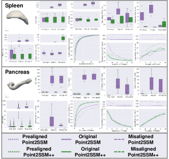
Figure 19: Point2SSM and Point2SSM++ results on prealigned, original, and misaligned data.

The results are provided in Fig. 19. Point2SSM and Point2SSM++ achieve similar accuracy on the test dataset that is aligned to match the training data. However, the accuracy of Point2SSM significantly decreases when the test datasets are not prealigned. Point2SSM++ achieves similar accuracy on all three versions of the test datasets for both the spleen and pancreas. These results demonstrate the superiority of Point2SSM++ in handling misaligned input.

Appendix D Additional Modes of Variation

The modes of variation for all comparison models on the single anatomy experiments are provided in Fig. 20. The reconstructed meshes resulting from the SC3K model have the most artifacts, indicating miscorrespondence. Some artifacts can also be seen in the ISR and DPC mesh reconstructions. The modes of variation are generally similar to those captured by the PSM and Point2SSM++ models (shown in Fig. 5). Overall, Point2SSM++ provides the smoothest and most interpretable modes of variation.

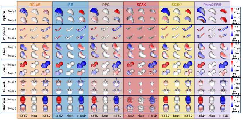
Figure 20: Primary and secondary modes of population variation captured by comparison methods across each dataset. The mean and shapes at $\pm 1.5$ standard deviation are shown with color denoting the distance to the mean. Blue indicates the surface is outside the mean, and red indicates the surface is inside the mean. Separate color scales and orientation markers are provided for each dataset.

References

- [1] A. L. Clouthier, J. Wenghofer, E. K. Wai, and R. B. Graham, “Morphable models of the lumbar spine to vary geometry based on pathology, demographics, and anatomical measurements,” Journal of Biomechanics, vol. 146, p. 111421, 2023.
- [2] P. R. Atkins, S. Y. Elhabian, P. Agrawal, M. D. Harris, R. T. Whitaker, J. A. Weiss, C. L. Peters, and A. E. Anderson, “Quantitative comparison of cortical bone thickness using correspondence-based shape modeling in patients with cam femoroacetabular impingement,” Journal of Orthopaedic Research, vol. 35, no. 8, pp. 1743–1753, 2017.
- [3] M. Soufi, Y. Otake, M. Hori, K. Moriguchi, Y. Imai, Y. Sawai, T. Ota, N. Tomiyama, and Y. Sato, “Liver shape analysis using partial least squares regression-based statistical shape model: application for understanding and staging of liver fibrosis,” International Journal of Computer Assisted Radiology and Surgery, vol. 14, pp. 2083–2093, 2019.
- [4] M. Schaufelberger, R. P. Kühle, A. Wachter, F. Weichel, N. Hagen, F. Ringwald, U. Eisenmann, J. Hoffmann, M. Engel, C. Freudlsperger et al., “A statistical shape model for radiation-free assessment and classification of craniosynostosis,” arXiv preprint arXiv:2201.03288, 2022.
- [5] D. Abler, S. Berger, A. Terrier, F. Becce, A. Farron, and P. Büchler, “A statistical shape model to predict the premorbid glenoid cavity,” Journal of shoulder and elbow surgery, vol. 27, no. 10, pp. 1800–1808, 2018.
- [6] E. M. van Es, F. Stockmans, and J. W. Colaris, “Corrective osteotomy in a patient with congenital absence of pronation based on three-dimensional statistical shape modeling,” HAND, p. 15589447231209343, 2023.
- [7] P. Friedrich, J. Wolleb, F. Bieder, F. M. Thieringer, and P. C. Cattin, “Point cloud diffusion models for automatic implant generation,” in International Conference on Medical Image Computing and Computer-Assisted Intervention. Springer, 2023, pp. 112–122.
- [8] V. Sciortino, T. Ingrassia, D. Cerniglia, and S. Pasta, “Statistical shape modelling as a tool for medical reverse engineering,” in International Conference of the Italian Association of Design Methods and Tools for Industrial Engineering. Springer, 2023, pp. 215–223.
- [9] L. H. Timmins, H. Samady, and J. N. Oshinski, “Effect of regional analysis methods on assessing the association between wall shear stress and coronary artery disease progression in the clinical setting,” in Biomechanics of Coronary Atherosclerotic Plaque. Elsevier, 2021, pp. 203–223.
- [10] P. Treleaven and J. Wells, “3d body scanning and healthcare applications,” Computer, vol. 40, no. 7, pp. 28–34, 2007.
- [11] C. R. Qi, H. Su, K. Mo, and L. J. Guibas, “Pointnet: Deep learning on point sets for 3d classification and segmentation,” in Proceedings of the IEEE conference on computer vision and pattern recognition, 2017, pp. 652–660.
- [12] Y. Guo, H. Wang, Q. Hu, H. Liu, L. Liu, and M. Bennamoun, “Deep learning for 3d point clouds: A survey,” IEEE transactions on pattern analysis and machine intelligence, vol. 43, no. 12, pp. 4338–4364, 2020.
- [13] A. Xiao, J. Huang, D. Guan, X. Zhang, S. Lu, and L. Shao, “Unsupervised point cloud representation learning with deep neural networks: A survey,” IEEE Transactions on Pattern Analysis and Machine Intelligence, 2023.
- [14] N. Chen, L. Liu, Z. Cui, R. Chen, D. Ceylan, C. Tu, and W. Wang, “Unsupervised learning of intrinsic structural representation points,” in Proceedings of the IEEE/CVF conference on computer vision and pattern recognition, 2020, pp. 9121–9130.
- [15] I. Lang, D. Ginzburg, S. Avidan, and D. Raviv, “Dpc: Unsupervised deep point correspondence via cross and self construction,” in 2021 International Conference on 3D Vision (3DV). IEEE, 2021, pp. 1442–1451.
- [16] J. Adams and S. Elhabian, “Point2SSM: Learning Morphological Variations of Anatomies from Point Clouds,” in The Twelfth International Conference on Learning Representations, 2024. [Online]. Available: https://openreview.net/forum?id=DqziS8DG4M
- [17] I. L. Dryden and K. V. Mardia, Statistical shape analysis: with applications in R. John Wiley & Sons, 2016, vol. 995.
- [18] J. Cates, P. T. Fletcher, M. Styner, M. Shenton, and R. Whitaker, “Shape modeling and analysis with entropy-based particle systems,” in IPMI. Springer, 2007, pp. 333–345.
- [19] R. H. Davies, C. J. Twining, T. F. Cootes, J. C. Waterton, and C. J. Taylor, “A minimum description length approach to statistical shape modeling,” IEEE transactions on medical imaging, vol. 21, no. 5, pp. 525–537, 2002.
- [20] M. Ovsjanikov, M. Ben-Chen, J. Solomon, A. Butscher, and L. Guibas, “Functional maps: a flexible representation of maps between shapes,” ACM Transactions on Graphics (ToG), vol. 31, no. 4, pp. 1–11, 2012.
- [21] M. Styner, I. Oguz, S. Xu, C. Brechbühler, D. Pantazis, J. J. Levitt, M. E. Shenton, and G. Gerig, “Framework for the statistical shape analysis of brain structures using spharm-pdm,” The insight journal, p. 242, 2006.
- [22] J. Cates, S. Elhabian, and R. Whitaker, “Shapeworks: particle-based shape correspondence and visualization software,” in Statistical shape and deformation analysis. Elsevier, 2017, pp. 257–298.
- [23] A. Goparaju, K. Iyer, A. Bone, N. Hu, H. B. Henninger, A. E. Anderson, S. Durrleman, M. Jacxsens, A. Morris, I. Csecs et al., “Benchmarking off-the-shelf statistical shape modeling tools in clinical applications,” Medical Image Analysis, vol. 76, p. 102271, 2022.
- [24] M. Datar, J. Cates, P. T. Fletcher, S. Gouttard, G. Gerig, and R. Whitaker, “Particle based shape regression of open surfaces with applications to developmental neuroimaging,” in International Conference on Medical Image Computing and Computer-Assisted Intervention. Springer, 2009, pp. 167–174.
- [25] J. Adams, N. Khan, A. Morris, and S. Elhabian, “Spatiotemporal Cardiac Statistical Shape Modeling: A Data-Driven Approach,” in International Workshop on Statistical Atlases and Computational Models of the Heart (STACOM), Held in Conjunction with MICCAI 2022, Proceedings. Springer, 2022, pp. 143–156.
- [26] ——, “Learning Spatiotemporal Statistical Shape Models for Non-Linear Dynamic Anatomies,” Frontiers in Bioengineering and Biotechnology, vol. 11, p. 1086234, 2023.
- [27] R. Bhalodia, S. Elhabian, J. Adams, W. Tao, L. Kavan, and R. Whitaker, “Deepssm: A blueprint for image-to-shape deep learning models,” Medical Image Analysis, vol. 91, p. 103034, 2024.
- [28] J. Adams, R. Bhalodia, and S. Elhabian, “Uncertain-deepssm: From images to probabilistic shape models,” Shape in Medical Imaging : International Workshop, ShapeMI 2020, Held in Conjunction with MICCAI 2020, Lima, Peru, October 4, 2020, Proceedings, vol. 12474, pp. 57–72, 2020.
- [29] J. Adams and S. Elhabian, “From images to probabilistic anatomical shapes: A deep variational bottleneck approach,” in Medical Image Computing and Computer Assisted Intervention–MICCAI 2022: 25th International Conference, Singapore, September 18–22, 2022, Proceedings, Part II. Springer, 2022, pp. 474–484.
- [30] J. Adams and S. Y. Elhabian, “Fully bayesian vib-deepssm,” in International Conference on Medical Image Computing and Computer-Assisted Intervention. Springer, 2023, pp. 346–356.
- [31] J. Ukey and S. Elhabian, “Localization-aware deep learning framework for statistical shape modeling directly from images,” in Medical Imaging with Deep Learning, 2023.
- [32] H. Xu and S. Y. Elhabian, “Image2ssm: Reimagining statistical shape models from images with radial basis functions,” arXiv preprint arXiv:2305.11946, 2023.
- [33] K. Iyer and S. Y. Elhabian, “Mesh2ssm: From surface meshes to statistical shape models of anatomy,” in International Conference on Medical Image Computing and Computer-Assisted Intervention. Springer, 2023, pp. 615–625.
- [34] J. Adams and S. Y. Elhabian, “Can point cloud networks learn statistical shape models of anatomies?” in International Conference on Medical Image Computing and Computer-Assisted Intervention. Springer, 2023, pp. 486–496.
- [35] A. Hornung, K. M. Wurm, M. Bennewitz, C. Stachniss, and W. Burgard, “Octomap: An efficient probabilistic 3d mapping framework based on octrees,” Autonomous robots, vol. 34, pp. 189–206, 2013.
- [36] M. Nießner, M. Zollhöfer, S. Izadi, and M. Stamminger, “Real-time 3d reconstruction at scale using voxel hashing,” ACM Transactions on Graphics (ToG), vol. 32, no. 6, pp. 1–11, 2013.
- [37] Y. Wang, Y. Sun, Z. Liu, S. E. Sarma, M. M. Bronstein, and J. M. Solomon, “Dynamic graph cnn for learning on point clouds,” Acm Transactions On Graphics (tog), vol. 38, no. 5, pp. 1–12, 2019.
- [38] H. Fan, X. Yu, Y. Yang, and M. Kankanhalli, “Deep hierarchical representation of point cloud videos via spatio-temporal decomposition,” IEEE Transactions on Pattern Analysis and Machine Intelligence, vol. 44, no. 12, pp. 9918–9930, 2021.
- [39] H. Fan, X. Yu, Y. Ding, Y. Yang, and M. Kankanhalli, “Pstnet: Point spatio-temporal convolution on point cloud sequences,” arXiv preprint arXiv:2205.13713, 2022.
- [40] H. Zhao, L. Jiang, J. Jia, P. H. Torr, and V. Koltun, “Point transformer,” in Proceedings of the IEEE/CVF international conference on computer vision, 2021, pp. 16 259–16 268.
- [41] X. Yu, L. Tang, Y. Rao, T. Huang, J. Zhou, and J. Lu, “Point-bert: Pre-training 3d point cloud transformers with masked point modeling,” in Proceedings of the IEEE/CVF Conference on Computer Vision and Pattern Recognition, 2022, pp. 19 313–19 322.
- [42] Y. Sun, Y. Wang, Z. Liu, J. Siegel, and S. Sarma, “Pointgrow: Autoregressively learned point cloud generation with self-attention,” in Proceedings of the IEEE/CVF Winter Conference on Applications of Computer Vision, 2020, pp. 61–70.
- [43] J. Wang, Y. Cui, D. Guo, J. Li, Q. Liu, and C. Shen, “Pointattn: You only need attention for point cloud completion,” arXiv preprint arXiv:2203.08485, 2022.
- [44] T. Deprelle, T. Groueix, M. Fisher, V. Kim, B. Russell, and M. Aubry, “Learning elementary structures for 3d shape generation and matching,” Advances in Neural Information Processing Systems, vol. 32, 2019.
- [45] L. Cosmo, E. Rodola, J. Masci, A. Torsello, and M. M. Bronstein, “Matching deformable objects in clutter,” in 2016 Fourth international conference on 3D vision (3DV). IEEE, 2016, pp. 1–10.
- [46] Y. Zeng, Y. Qian, Z. Zhu, J. Hou, H. Yuan, and Y. He, “Corrnet3d: Unsupervised end-to-end learning of dense correspondence for 3d point clouds,” in Proceedings of the IEEE/CVF Conference on Computer Vision and Pattern Recognition, 2021, pp. 6052–6061.
- [47] S. Suwajanakorn, N. Snavely, J. J. Tompson, and M. Norouzi, “Discovery of latent 3d keypoints via end-to-end geometric reasoning,” Advances in neural information processing systems, vol. 31, 2018.
- [48] C. Fernandez-Labrador, A. Chhatkuli, D. P. Paudel, J. J. Guerrero, C. Demonceaux, and L. V. Gool, “Unsupervised learning of category-specific symmetric 3d keypoints from point sets,” in Computer Vision–ECCV 2020: 16th European Conference, Glasgow, UK, August 23–28, 2020, Proceedings, Part XXV 16. Springer, 2020, pp. 546–563.
- [49] T. Jakab, R. Tucker, A. Makadia, J. Wu, N. Snavely, and A. Kanazawa, “Keypointdeformer: Unsupervised 3d keypoint discovery for shape control,” in Proceedings of the IEEE/CVF Conference on Computer Vision and Pattern Recognition, 2021, pp. 12 783–12 792.
- [50] A.-C. Cheng, X. Li, M. Sun, M.-H. Yang, and S. Liu, “Learning 3d dense correspondence via canonical point autoencoder,” Advances in Neural Information Processing Systems, vol. 34, pp. 6608–6620, 2021.
- [51] M. Zohaib and A. Del Bue, “Sc3k: Self-supervised and coherent 3d keypoints estimation from rotated, noisy, and decimated point cloud data,” in Proceedings of the IEEE/CVF International Conference on Computer Vision, 2023, pp. 22 509–22 519.
- [52] H. Fan, X. Yu, Y. Yang, and M. Kankanhalli, “Deep hierarchical representation of point cloud videos via spatio-temporal decomposition,” IEEE Transactions on Pattern Analysis and Machine Intelligence, vol. 44, no. 12, pp. 9918–9930, 2021.
- [53] P. He, P. Emami, S. Ranka, and A. Rangarajan, “Learning canonical embeddings for unsupervised shape correspondence with locally linear transformations,” IEEE Transactions on Pattern Analysis and Machine Intelligence, 2023.
- [54] T. Nguyen, Q.-H. Pham, T. Le, T. Pham, N. Ho, and B.-S. Hua, “Point-set distances for learning representations of 3d point clouds,” in Proceedings of the IEEE/CVF international conference on computer vision, 2021, pp. 10 478–10 487.
- [55] N. Tishby, F. C. Pereira, and W. Bialek, “The information bottleneck method,” 2000.
- [56] J. C. Gower, “Generalized procrustes analysis,” Psychometrika, vol. 40, pp. 33–51, 1975.
- [57] B. C. Munsell, P. Dalal, and S. Wang, “Evaluating shape correspondence for statistical shape analysis: A benchmark study,” IEEE Transactions on Pattern Analysis and Machine Intelligence, vol. 30, no. 11, pp. 2023–2039, 2008.
- [58] A. L. Simpson, M. Antonelli, S. Bakas, M. Bilello, K. Farahani, B. Van Ginneken, A. Kopp-Schneider, B. A. Landman, G. Litjens, B. Menze et al., “A large annotated medical image dataset for the development and evaluation of segmentation algorithms,” arXiv preprint arXiv:1902.09063, 2019.
- [59] J. Ma, Y. Zhang, S. Gu, C. Zhu, C. Ge, Y. Zhang, X. An, C. Wang, Q. Wang, X. Liu, S. Cao, Q. Zhang, S. Liu, Y. Wang, Y. Li, J. He, and X. Yang, “Abdomenct-1k: Is abdominal organ segmentation a solved problem?” IEEE Transactions on Pattern Analysis and Machine Intelligence, vol. 44, no. 10, pp. 6695–6714, 2022.
- [60] A. Sekuboyina, M. E. Husseini, A. Bayat, M. Löffler, H. Liebl, H. Li, G. Tetteh, J. Kukačka, C. Payer, D. Štern et al., “Verse: a vertebrae labelling and segmentation benchmark for multi-detector ct images,” Medical image analysis, vol. 73, p. 102166, 2021.
- [61] P. Achlioptas, O. Diamanti, I. Mitliagkas, and L. Guibas, “Learning representations and generative models for 3d point clouds,” in International conference on machine learning. PMLR, 2018, pp. 40–49.
- [62] C. R. Qi, L. Yi, H. Su, and L. J. Guibas, “Pointnet++: Deep hierarchical feature learning on point sets in a metric space,” Advances in neural information processing systems, vol. 30, 2017.
- [63] J. Wasserthal, H.-C. Breit, M. T. Meyer, M. Pradella, D. Hinck, A. W. Sauter, T. Heye, D. T. Boll, J. Cyriac, S. Yang et al., “Totalsegmentator: Robust segmentation of 104 anatomic structures in ct images,” Radiology: Artificial Intelligence, vol. 5, no. 5, 2023.
- [64] A. Morris, E. Kholmovski, N. Marrouche, J. Cates, and S. Elhabian, “An image-based approach for 3d left atrium functional measurements,” in 2020 Computing in Cardiology. IEEE, 2020, pp. 1–4.