Time-connected phase slips in current-driven two-band superconducting wires

Abstract

We study quasi-one dimensional wires of two-band superconductors driven by an electrical current. We find that the onset of dissipation can occur with the nucleation of time-connected phase slips (t-PS). The topological structure of the t-PS consists of two phase slips (one in each order parameter) separated in time and connected via an interband vortex string along the time direction. This shows as a two-peak structure in voltage vs. time. We discuss the conditions for observing t-PS, depending on the interband coupling strength and the relaxation time scales for each order parameter.

I Introduction

Abrikosov vortices abrikosov in superconductors are topological singularities where the superconducting order parameter $\Psi=|\Psi|e^{i\theta}$ vanishes at a point in space (actually, in a line of points in three dimensions) and the phase $\theta$ changes by $2\pi n$ around a closed loop that encircles the vortex, $\oint d\theta=2\pi n$. The integer $n$ defines the “vorticity” associated to the topological singularity. Vortices nucleate in type II superconductors tinkham in the presence of a magnetic field $\mathbf{B}$, which determines the vortex density. Another interesting case of topological singularities occurs in quasi one-dimensional superconducting wires. When driven by a current, the onset of voltage usually occurs through the nucleation of phase-slips (PS) skocpol1974 ; kramer1977 ; kramer1978 ; ivlev1978 ; ivlev1980 ; watts-tobin1981 ; ivlev1984 ; kopnin2001 . The superconducting order parameter $\Psi=|\Psi|e^{i\theta}$ vanishes in a point in the wire (the PS center) at a given time, after which it recovers a finite value, and this process repeats periodically. Throughout each of these events in time the phase $\theta$ changes by $2\pi$. Ivlev and Kopnin ivlev1978 have shown that the PS are vortices in space-time. Phase increments $d\theta$, integrated along a closed loop in space and time around a PS give $\oint_{\rm space-time}d\theta=2\pi$. Thus, PS are topological singularities in two-dimensional space-time. The electric field $E$ (instead of $B$) determines their density in time ivlev1978 , i.e. the number of PS per unit time. The dynamics of PS and the current-voltage curves in superconducting wires have been studied in detail both theoretically and experimentally since the 1970s skocpol1974 ; kramer1977 ; kramer1978 ; ivlev1978 ; ivlev1980 ; watts-tobin1981 ; ivlev1984 ; kopnin2001 ; michotte2004 . The dynamics of PS can be modeled with the time dependent Ginzburg-Landau (TDGL) equation kramer1977 . There is nowadays a good understanding of the dependence of the PS dynamics on TDGL parameters, wire size and boundary conditions michotte2004 ; vodolazov2011 ; ludac2008 ; kim2010 ; baranov2011 ; baranov2013 ; kallush2014 ; berger2015 ; kimmel2017 . Recent experiments in nanowires have achieved detailed control and manipulation of the PS, with pulses of electrical current buh2015 , with infrared laser pulses madan2018 , and with microwave radiation kato2020 .

In the last two decades, the discovery of multiband superconductivity in MgB₂ choi2002 , and later on in materials such as NbSe₂boaknin2003 , OsB₂singh2010 , FeSe_0.94 khasanov2010 , LiFeAs Kim2011 and other iron-pnictide superconductors, has stimulated the study of the physics of vortices with nontrivial topological properties babaev2002 . For instance, two-band superconductors are described with two order parameters $\Psi_{j}=|\Psi_{j}|e^{i\theta_{j}}$, $j=1,2$. Therefore, the topological singularities of the two order parameters have to be considered, $\oint d\theta_{1}=2\pi n_{1}$ and $\oint d\theta_{2}=2\pi n_{2}$ babaev2002 ; smorgrav2005 . The simplest case consists of composite vortices centered at the same point with $n_{1}=n_{2}$ , which are encountered in the equilibrium sates in two-band bulk superconductors under a magnetic field. The so-called non-composite vortices are topological singularities displaced in space ($n_{1}\not=n_{2}$ in each point) which are associated with fractional magnetic flux quanta babaev2002 . They can appear in finite mesoscopic samples chibotaru2007 ; geurts2010 ; pina2012 ; silva2014 , at the sample boundaries silaev2011 , and in samples driven at high currents lin2013 ; mosquera2017 .

In one-dimensional two-band superconducting wires the existence of phase textures and topological solitons of the interband phase difference $\theta_{2}-\theta_{1}$ has been extensively studied tanaka2001 ; gurevich2003b ; gurevich2006 ; yerin2007 ; lin2012 ; fenchenko2012 ; lin2014 ; tanaka2015 ; tanaka2015b ; marychev2018 ; berger2011 . In the soliton states the phase difference $\theta_{2}-\theta_{1}$ varies with the space coordinate and rotates in multiples of $2\pi$ along the wire length tanaka2001 . The phase solitons are induced by a finite driving current below the critical current of the wire. One nucleation mechanism can be charge imbalance at the boundary between the superconducting wire and a normal lead gurevich2003b . The number of phase solitons depends on the driving current and the wire length marychev2018 .

In this work we address the dynamics of two-band superconducting wires at the onset of dissipation, above their critical current. We analyze the topological nature of the induced phase slips and their dependence on interband coupling strength by solving numerically a time dependent two-band Ginzburg-Landau equation. We find that the induced PS in the two bands nucleate at the same place but are separated in time. They are connected through a topological singularity in the interband phase difference that is oriented along the time direction, and we name these nontrivial topological objects as “time-connected phase slips” (t-PS). The paper is organized as follows. In Section II we introduce the time-dependent Ginzburg-Landau equations to be solved, boundary conditions and parameters to be considered. In Section III we report our results for the current-voltage curves and characterize the space and time dependence of the induced PS. In Section IV the topological nature of the t-PS is described in detail and in Section V we report their dependence on interband coupling and relaxation parameters. Finally, in Section VI we summarize and discuss our findings.

II Model and definitions

For a two-component superconductor, the free energy is ${\cal F}=\int d^{3}{\bf r}f({\bf r})$ zhitomirsky2004 ; gurevich2003 ; koshelev2005 with

$$f= \alpha_{1}\left|\Psi_{1}\right|^{2}+\frac{\beta_{1}}{2}\left|\Psi_{1}\right|^{4}+\frac{1}{2m_{1}}\left|\left(-i\hbar\nabla-\frac{2e}{c}\mathbf{A}\right)\Psi_{1}\right|^{2}+$$

$$\alpha_{2}\left|\Psi_{2}\right|^{2}+\frac{\beta_{2}}{2}\left|\Psi_{2}\right|^{4}+\frac{1}{2m_{2}}\left|\left(-i\hbar\nabla-\frac{2e}{c}\mathbf{A}\right)\Psi_{2}\right|^{2}+$$

$$\frac{|\mathbf{B}|^{2}}{8\pi}-\gamma\left(\Psi_{1}\Psi_{2}^{*}+\Psi_{2}\Psi_{1}^{*}\right)$$

where $\alpha_{1},\alpha_{2},\beta_{1},\beta_{2},m_{1},m_{2}$ are the Ginzburg-Landau expansion coefficients, ${\bf A}$ is the vector potential, ${\bf B}$ is the magnetic field, and $\gamma$ is the interband Josephson coupling parameter.

We study the dynamics near the critical temperature $T\lesssim T_{c}$ using the time-dependent Ginzburg-Landau equations generalized to a two-band superconductor vargunin2020 ; gurevich2003b ; gurevich2006 ; berger2011 ; fenchenko2012 ; marychev2018 ; mosquera2017 :

$$\Gamma_{1}\left(\frac{\partial}{\partial t}+i\frac{2e}{\hbar}\phi\right)\Psi_{1}=-\frac{\delta{\cal F}}{\delta\Psi_{1}^{*}}$$

$$\Gamma_{2}\left(\frac{\partial}{\partial t}+i\frac{2e}{\hbar}\phi\right)\Psi_{2}=-\frac{\delta{\cal F}}{\delta\Psi_{2}^{*}}$$ (1)

$${\bf J}=-\sigma\left(\nabla\phi+\frac{1}{c}\frac{\partial\mathbf{A}}{\partial t}\right)$$

$$~{}~{}+\frac{2e\hbar}{m_{1}}\operatorname{Im}\left(\Psi_{1}^{*}[\nabla-i(2e/\hbar c)\mathbf{A}]\Psi_{1}\right)$$

$$~{}~{}+\frac{2e\hbar}{m_{2}}\operatorname{Im}\left(\Psi_{2}^{*}[\nabla-i(2e/\hbar c)\mathbf{A}]\Psi_{2}\right)$$

where $\Gamma_{i}=\frac{\hbar^{2}}{2m_{i}D_{i}}$ with $D_{i}$ the diffusion coefficients, $\sigma$ is the normal conductivity, $\phi$ is the electric potential, and ${\bf J}$ the electric current density. We will take ${\bf A}=0$, since there is no applied external magnetic fields and the effect of the self-induced magnetic field in the one-dimensional wire is negligible.

We normalize $\Psi_{i}$ by $\Psi_{10}=\sqrt{-\alpha_{1}/\beta_{1}}$, length scale by $\xi_{1}=\sqrt{\hbar^{2}/2m_{1}(-\alpha_{1})}$, time by $t_{0}=4\pi\sigma\lambda_{1}^{2}/c^{2}=\sigma m_{1}\beta_{1}/2e^{2}(-\alpha_{1})$, electric potential $\phi$ by $v_{0}=\hbar/2et_{0}$ and current density $J$ by $J_{0}=\hbar\sigma/2et_{0}\xi_{1}$. With this normalization the TDGL equations in a one-dimensional wire are:

$$\eta_{1}\left(\frac{\partial}{\partial t}+i\phi\right)\Psi_{1}=\frac{\partial^{2}\Psi_{1}}{\partial x^{2}}+\left(1-\left|\Psi_{1}\right|^{2}\right)\Psi_{1}+g\Psi_{2}$$ (2)

$$\eta_{2}\left(\frac{\partial}{\partial t}+i\phi\right)\Psi_{2}=k\frac{\partial^{2}\Psi_{2}}{\partial x^{2}}+\left(a-b\left|\Psi_{2}\right|^{2}\right)\Psi_{2}+g\Psi_{1}$$

and

$$J=-\frac{\partial\phi}{\partial x}+\operatorname{Im}\left(\Psi_{1}^{*}\frac{\partial\Psi_{1}}{\partial x}\right)+k\operatorname{Im}\left(\Psi_{2}^{*}\frac{\partial\Psi_{2}}{\partial x}\right)$$ (4)

with $a=\alpha_{2}/\alpha_{1}$, $b=\beta_{2}/\beta_{1}$, $g=\gamma/|\alpha_{1}|$, $k=m_{1}/m_{2}$, $\eta_{i}=\Gamma_{i}/t_{0}|\alpha_{1}|$; we also define $d=D_{1}/D_{2},$ and thus $\eta_{2}=kd\eta_{1}$.

We use the convention that $\Psi_{1}$ corresponds to the ‘strong’ band and $\Psi_{2}$ to the ‘weak’ band and consider the case that both bands are superconducting, meaning that $\alpha_{1}(T)<\alpha_{2}(T)<0$, and thus $0<a<1$. Also, for consistency with the ‘weak’ band choice, we consider parameters such that the second band has smaller equilibrium gap, $(\Psi_{20}/\Psi_{10})^{2}=a/b<1$ and larger coherence length, $\xi_{2}^{2}/\xi_{1}^{2}=k/a>1$. Furthermore, weak interband coupling means $\gamma<|\alpha_{2}|<|\alpha_{1}|$, i.e. $g<a<1$. In contrast to single-band superconductors for which the relaxation constant is $\eta\approx 5.79$ kramer1977 ; kramer1978 ; ivlev1984 , in multiband superconductors the relaxation constants $\eta_{1},\eta_{2}$ depend strongly on system parameters vargunin2020 . The ratio $\eta_{2}/\eta_{1}=kd$ depends on the ratio of diffusivities $d=D_{1}/D_{2}$, which has been found to vary significantly on different superconducting compounds dai2011 ; vargunin2020 (typically in the range $0.1\lesssim d\lesssim 10$). The relaxation times of the order parameters are $t_{i}=\Gamma_{i}/|\alpha_{i}|$, which in terms of the normalization $t_{0}$ are $t_{1}/t_{0}=\eta_{1}$ and $t_{2}/t_{0}=\eta_{2}/a$, and the ratio of these time scales is $t_{2}/t_{1}=kd/a$. Here we will focus on the case $\eta_{2}/a>1$ and $\eta_{1}<1$, i.e. the weak band order parameter has a large relaxation time while the strong band has fast relaxation.

We integrate numerically Eq.(2) with a semi-implicit Crank-Nicholson algorithm (see Appendix for details), with $\delta t=0.02$ and $\delta x=0.25$. We consider superconducting wires of length $L$ with a superconducting bank boundary condition:

$$\Psi_{j}(x=0,t) = \Delta_{j}e^{-i\int_{0}^{t}\phi(0,t^{\prime})dt^{\prime}}$$ (5)

$$\Psi_{j}(x=L,t) = \Delta_{j}e^{-i\int_{0}^{t}\phi(L,t^{\prime})dt^{\prime}}$$

where $\Delta_{j}=\Psi_{j}^{\rm eq}$ is the equilibrium order parameter of the $j$-band at zero current, obtained numerically by solving the equilibrium homogeneous equations,

$$\left(1-|\Delta_{1}|^{2}\right)\Delta_{1}+g\Delta_{2} = 0$$

$$\left(a-b|\Delta_{2}|^{2}\right)\Delta_{2}+g\Delta_{1} = 0$$

For fixed current density $J$, $\phi(x,t)$ is found by direct integration of Eq. (4), with the additional knowledge that $\partial\phi/\partial x=0$ at $x=0,L$. The time dependent voltage drop per unit length is determined as $v(t)=[\phi(0,t)-\phi(L,t)]/L$.

III Current-voltage curves and nucleation of phase slips

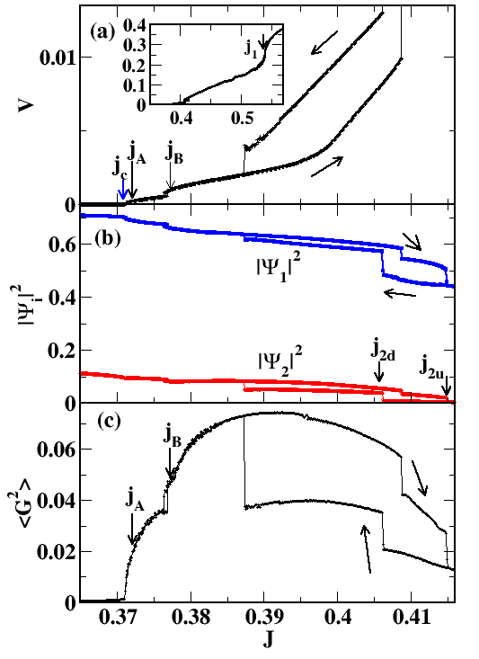
Figure 1: (a) IV curve for a wire of length $L=50\xi_{1}$. $V$ is the average voltage per unit length normalized by $v_{0}/\xi_{1}$ and the current $J$ is normalized by $J_{0}$. The onset of dissipation at $j_{c}$ is indicated. The inset shows the curve in a wider range of currents, where $j_{1}$ indicates the current for which the wire becomes normal. (b) Average order parameters $|\Psi_{1}|^{2}$ (blue line) and $|\Psi_{2}|^{2}$ (red line) as functions of $J$. (c) Measure of interband phase texture $\langle G^{2}\rangle$ (see text for definition) as a function of $J$. System parameters: $a=0.2$, $b=1.2$, $k=5.2$, $g=0.08$, $\eta_{1}=0.5$, $\eta_{2}=5.2$. The current $j_{A}$ corresponds to the case shown in Fig.2 and $j_{B}$ corresponds to the case shown in Fig.3(a). In (b) and (c), $|\Psi_{1}|^{2}$, $|\Psi_{2}|^{2}$ and $\langle G^{2}\rangle$ are normalized by $\Psi_{10}^{2}$.

We first calculate the current-voltage (IV) curves for $a=0.2$, $b=1.2$, $k=5.2$, $g=0.08$, $\eta_{1}=0.5$ and $\eta_{2}=5.2$. We simulate the dynamics ramping up and ramping down the external current $J$ for wires of length $L=50\xi_{1}$. We start with the equilibrium values of $\Psi_{i}(x)$ at $J=0$ and increase gradually the current, taking as initial condition the final values of $\Psi_{i}(x)$ at the previous current step. After reaching the normal state, we lower the current back to $J=0$, following the same procedure.

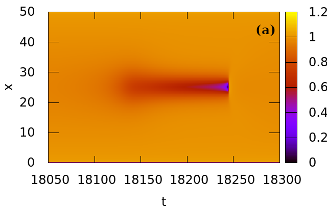
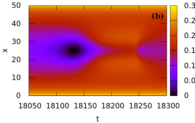
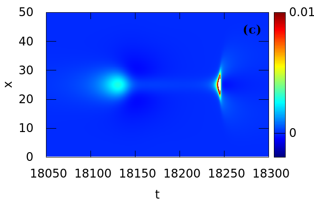
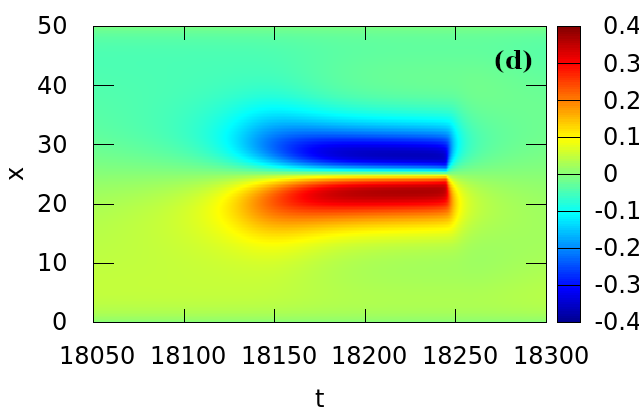
Figure 2: Intensity plots in space-time coordinates showing the structure of phase slips for a current $J=0.372\gtrsim j_{c}$ [indicated as $j_{A}$ in Fig.1(a)]. Order parameters (a) $|\Psi_{1}(x,t)|^{2}$ and (b) $|\Psi_{2}(x,t)|^{2}$, normalized by $\Psi_{10}^{2}$. (c) Electric field $E(x,t)=-\frac{\partial}{\partial x}\phi(x,t)$ normalized by $v_{0}/\xi_{1}$. (d) Interband phase texture $G(x,t)=|\Psi_{1}||\Psi_{2}|\sin(\theta_{1}-\theta_{2})$, normalized by $\Psi_{10}^{2}$. Coordinate $x$ is normalized by $\xi_{1}$ and time by $t_{0}$.

We have calculated numerically the time-averaged voltage per unit length $V=\langle v(t)\rangle$ [shown in Fig.1(a)], and the time and length averaged order parameters $\langle|\Psi_{i}|^{2}\rangle=\langle\frac{1}{L}\int_{0}^{L}|\Psi_{i}(x,t)|^{2}dx\rangle$, $i=1,2$ [shown in Fig.1(b)]. We find that there is an onset of dissipation at the current density $J=j_{c}$. Above $j_{c}$ the voltage increases, starting with a steep square root dependence ($V\propto\sqrt{J-j_{c}}$) michotte2004 ; baranov2011 followed by a quasilinear behavior. As we will show, this voltage onset corresponds to the nucleation of one phase slip in each band. Upon increasing the current there are further onsets of subsequent regions of quasilinear dependence, that correspond to increasing number of PS centers at more than one position. At a larger current, $J=j_{2u}$, the $2$-band becomes normal while the $1$-band is still superconducting. At an even higher current $j_{1}>j_{2u}$ the wire becomes completely normal in the bulk [note that $\Psi_{i}$ is always finite near the edges due to Eq.(5)]. The current $j_{1}$ is shown in the inset of Fig.1. As the current decreases, there is hysteresis and the $2$-band stays normal down to lower currents, becoming superconducting at a current $j_{2d}<j_{2u}$. Below $j_{2d}$ the voltage decreases with current, with a different sequence of quasilinear regions, showing a noticeable hysteresis.

We focus in the range $j_{c}<J<j_{2d}$, where there is a finite voltage while both bands are superconducting. In order to understand the nucleation of PS near the onset of dissipation, $J\gtrsim j_{c}$ , we study the order parameters $|\Psi_{1}(x,t)|^{2}$ and $|\Psi_{2}(x,t)|^{2}$ as functions of $x$ and $t$. We find that PS nucleate at the center of the wire, where each order parameter vanishes periodically in time. In Fig.2(a) and (b) we show $|\Psi_{1}(x,t)|^{2}$ and $|\Psi_{2}(x,t)|^{2}$ in a time window where both PS can be observed. The PS of the weak band (corresponding to $\Psi_{2}$) occurs earlier than the PS in which $\Psi_{1}$ vanishes. The PS vortex core for the $i$-band (region where the order parameter drops) has a length scale of the order of $\xi_{i}$ and a time scale of the order of $t_{i}$. Therefore, the core of the $\Psi_{2}$ phase slip is larger than the core of $\Psi_{1}$. The electric field $E(x,t)=-\partial\phi(x,t)/\partial x$ is plotted in Fig.2(c). Away from the PS the electric field is zero, $E\approx 0$, as expected. There are two maxima of significant $E$ at the cores of the PSs of each band. The maximum of $E$ in the 2-band is much smaller than the maximum in the 1-band. The characteristic time lag between these two PSs will be denoted $t_{\gamma}$ from now on.

Since superconductivity vanishes at different times in the two bands, we expect that the phases $\theta_{i}$ of the two order parameters will be different. To quantify the occurrence of interband phase textures we evaluate the interband “Josephson current”:

$$G(x,t) = \operatorname{Im}[\Psi_{1}(x,t)\Psi_{2}^{*}(x,t)]$$

$$= |\Psi_{1}(x,t)||\Psi_{2}(x,t)|\sin[\theta_{1}(x,t)-\theta_{2}(x,t)].$$

The total integrated interband current should be zero, $\int_{0}^{L}G(x,t)dx=0$, since there is no net current applied between bands gurevich2006 . When the two bands are phase-locked, i.e. $\theta_{2}(x,t)=\theta_{1}(x,t)$, $G(x,t)=0$ everywhere. On the other hand, if there are phase textures, $\int_{0}^{L}G^{2}(x,t)dx\not=0$. Therefore, as a measure of the interband texture, we calculate the time averaged $\langle G^{2}\rangle=\langle\frac{1}{L}\int_{0}^{L}G^{2}(x,t)dx\rangle$ [shown in Fig.1(c)]. We find that below $j_{c}$ the two bands are phase-locked (there are no phase textures in this case), but just above $j_{c}$ the interband“current” is finite, $\langle G^{2}\rangle>0$, indicating that there are phase differences $\theta_{2}-\theta_{1}$ induced by the driving current. The hysteresis in the voltage and in the order parameters is also reflected as a hysteresis in the $\langle G^{2}\rangle$ vs $J$ curve.

We also plot in Fig.2(d) the space-time distribution of the interband“current” $G(x,t)$ when there are PSs. Away from the PS the system is phase-locked and thus $G\approx 0$. At the time interval between the zeroes of $|\Psi_{2}(x,t)|^{2}$ and $|\Psi_{1}(x,t)|^{2}$, there is a phase texture where $G\not=0$. We note that this phase structure corresponds to a vortex string, which is coreless (there is no vanishing of the order parameter inside) and that it extends along the time direction, so we name it a“time-vortex”. As we will discuss in the upcoming sections, its characteristic time scale, $t_{\gamma}$, depends on the driving current and the interband coupling stregth $g$.

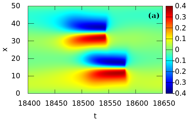
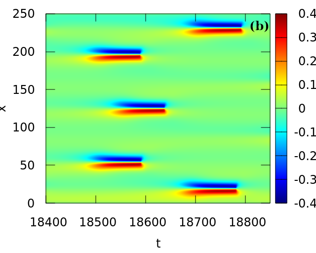
Figure 3: Intensity plots in space-time coordinates of the interband phase texture $G(x,t)=|\Psi_{1}||\Psi_{2}|\sin(\theta_{1}-\theta_{2})$, normalized by $\Psi_{10}^{2}$. Coordinate $x$ is normalized by $\xi_{1}$ and time by $t_{0}$. (a) $J=0.3772$ [indicated as $j_{B}$ in Fig.1], $L=50\xi_{1}$. (b) $J=0.3731$, $L=250\xi_{1}$.

At larger currents (but for $J<j_{2d}$), more PS centers can nucleate. In Fig.3(a) we show the case for a current in the range of the second quasilinear region in the current-voltage curve. We plot $G(x,t)$ showing that there are two centers with time-vortices that connect pairs of PS in the superconducting bands. Also if the wire length is increased, more slip centers can nucleate in the wire, as seen in Fig.3(b) for a wire of length $L=250\xi_{1}$.

IV Topological connection in time of the phase slips

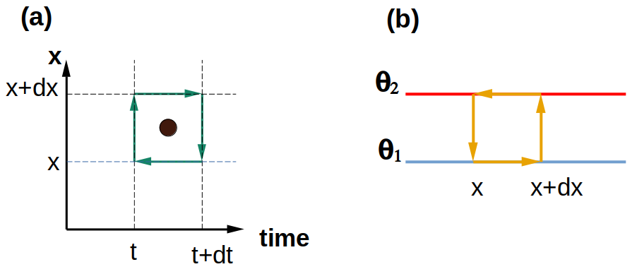
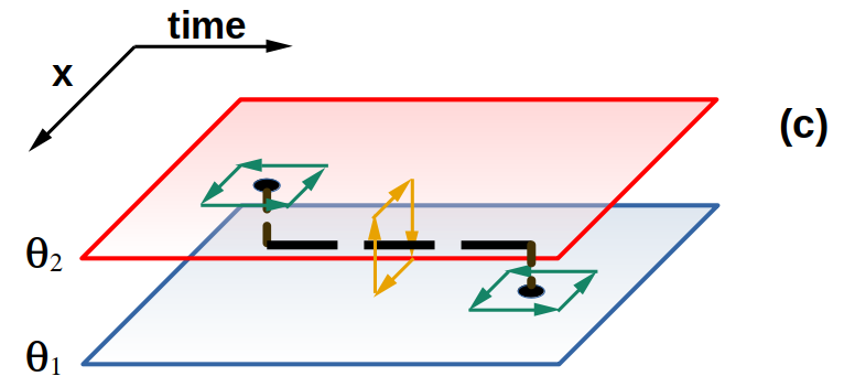
Figure 4: (a) Space-time loop for the calculation of the phase-slip vorticities $\nu_{i}(x,t)$, as defined in Eq.(7). (b) Space-interband loop for the calculation of the time-oriented interband vorticity $\nu_{\gamma}(x,t)$, as defined in Eq.(IV). (c) Schematic representation of the topological structure of a time-connected phase slip. The dimension perpendicular to the plane $xt$ is an abstract coordinate that assumes the values $\theta_{1}(x,t)$ in the lower plane and $\theta_{2}(x,t)$ in the upper plane.

Following Ivlev and Kopin ivlev1978 , we can regard a PS as a vortex (a topological singularity) in two-dimensional space-time. In each $i$-band, the sum of phase differences $\delta_{x}\theta_{i}$ and $\delta_{t}\theta_{i}$ along a closed loop in space-time must equal an integer multiple of $2\pi$. Accordingly, we define the PS vorticity as

$$\oint\frac{\partial\theta_{i}}{\partial{\vec{\rho}}}\cdot d{\vec{\rho}}={2\pi}\nu_{i}$$ (6)

with the space-time coordinate ${\vec{\rho}}=(x,t)$.

We can calculate local vorticities $\nu_{i}(x,t)$ considering infinitesimal loops along closed paths corresponding to the discretization distances $dx,dt$. In this case, the closed space-time line integral is obtained as a oriented sum along the four segments of the loop shown in Fig.4(a). In the spatial segments we obtain the phase differences $\delta_{x}\theta_{i}(x,t)$ from $x+dx$ to $x$ at $t$ fixed; and in the temporal segments we obtain the phase differences $\delta_{t}\theta_{i}(x,t)$ from $t+dt$ to $t$ at $x$ fixed. To calculate numerically the vorticity teitel1993 ; phillips2015 , the phase differences $\delta_{\mu}\theta_{i}$ ($\mu=x,t$) are redefined in the $(-\pi,\pi)$ interval as $\delta_{\mu}\theta_{i}\rightarrow[\delta_{\mu}\theta_{i}]=\delta_{\mu}\theta_{i}+2\pi m_{i,\mu}$, where the link integers are $m_{i,\mu}=-{\rm nint}(\frac{\delta_{\mu}\theta_{i}}{2\pi})$, with ${\rm nint}(u)$ the nearest integer of $u$. We then obtain,

$$\nu_{i}(\tilde{x},\tilde{t}) = m_{i,x}(x,t)+m_{i,t}(x+dx,t)$$ (7)

$$-m_{i,x}(x,t+dt)-m_{i,t}(x,t)$$

where the point ($\tilde{x},\tilde{t}$) is located in the interior of the considered rectangle. The integers $m_{i,x}(x,t)$ are defined in the directed link between $(x,t)$ and $(x+dx,t)$, meaning that when the summation path goes from $(x+dx,t)$ to $(x,t)$ they are added as $-m_{i,x}(x,t)$; similar convention is taken for the $m_{i,t}(x,t)$ integers.

In the two-band superconductor one can also define a vortex string (i.e. a “Josephson” vortex dremov2019 ), which is a $2\pi$-singularity in the phase difference $\Delta\theta=\theta_{2}-\theta_{1}$. In this way, it is possible to quantify comment an interband vorticity taking a closed loop that goes from a point $x_{a}$ to $x_{b}$ in the 1-band and returns from $x_{b}$ to $x_{a}$ in the 2-band, as

$$2\pi\nu_{\gamma}=\int_{x_{a}}^{x_{b}}\delta_{x}\theta_{1}+\Delta\theta(x_{b})-\int_{x_{a}}^{x_{b}}\delta_{x}\theta_{2}-\Delta\theta(x_{a})\;.$$ (8)

We can then calculate a local vorticity in a closed small path that goes from $x$ to $x+dx$ and back, see Fig.4(b), as

$$\nu_{\gamma}(\tilde{x},t) = m_{1,x}(x,t)+m_{\Delta}(x+dx,t)$$

$$-m_{2,x}(x,t)-m_{\Delta}(x,t)$$

where we have also restricted to the $(-\pi,\pi)$ interval the interband phase differences $\Delta\theta$, redefined as $\Delta\theta\rightarrow[\Delta\theta]=\Delta\theta+2\pi m_{\Delta}$, with the link integers $m_{\Delta}=-{\rm nint}(\frac{\Delta\theta}{2\pi})$.

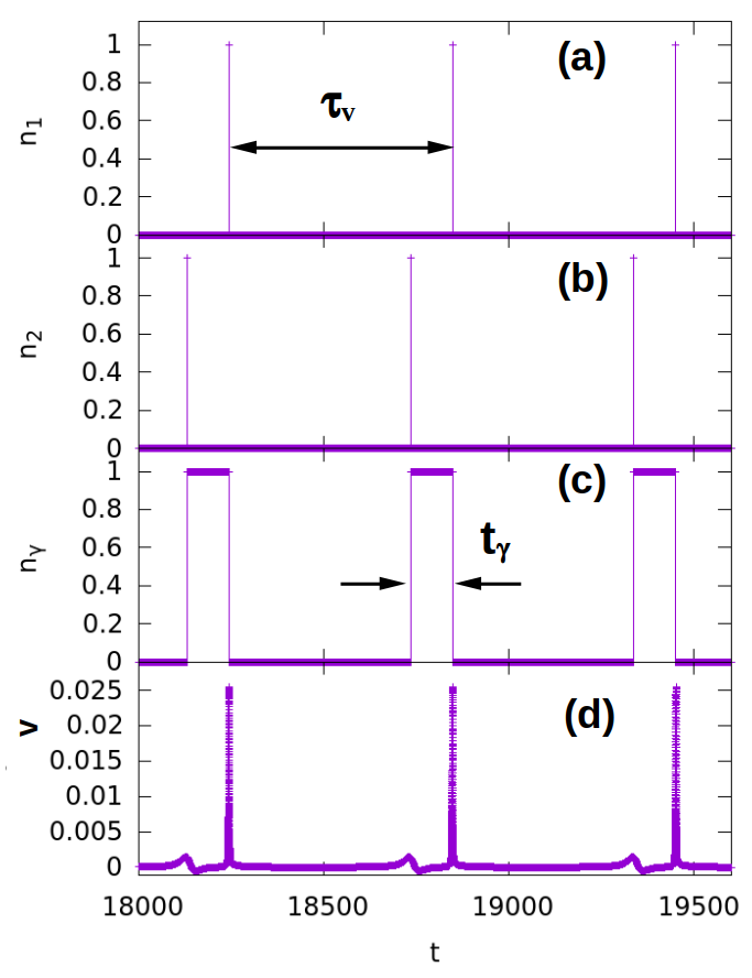
Figure 5: Time-dependence of the t-PS for a current $J=0.372$ [indicated as $j_{A}$ in Fig.1(a)] for a wire with $L=50\xi_{1}$. Phase-slip vorticities (a) $n_{1}$ and (b) $n_{2}$. (c) Interband vorticity $n_{\gamma}$. (d) Voltage per unit length $v$, normalized by $v_{0}/\xi_{1}$. Time is normalized by $t_{0}$.

We also define the total vorticities along the wire at a given time, both the phase-slip vorticities $n_{i}(t)=\sum_{x}\nu_{i}(x,t)$ and the interband vorticities $n_{\gamma}(t)=\sum_{x}\nu_{\gamma}(x,t)$. From Eq. (7), we can write

$$n_{i}(\tilde{t}) = \sum_{x}\left\{m_{i,x}(x,t)-m_{i,x}(x,t+dt)\right\}$$

$$+ m_{i,t}(L,t)-m_{i,t}(0,t)$$

where the sums are taken over the $L/dx$ segments in the grid. The second line in Eq. (IV) has the same value for the two bands, due to the boundary conditions Eq.(5) at $x=0$ and $x=L$. Similarly, from Eq.(IV) we obtain,

$$n_{\gamma}(\tilde{t}) = \sum_{x}\left\{m_{2,x}(x,t)-m_{1,x}(x,t)\right\}$$

$$+ m_{\Delta}(L,t)-m_{\Delta}(0,t)\,,$$

where the second line vanishes since $\theta_{2}=\theta_{1}$ at $x=0$ and $x=L$ due to Eq.(5). Combining Eqs.(IV) and (IV), it follows that

$$n_{\gamma}(\tilde{t}+dt)-n_{\gamma}(\tilde{t})=n_{2}(\tilde{t})-n_{1}(\tilde{t}).$$ (12)

We plot in Fig.5(a),(b),(c) the total vorticities as functions of the time. We see that, periodically, a phase-slip is created first in the“weak band” when $n_{2}=1$ at an instant of time (while $n_{1}=n_{\gamma}=0$). Right after this time, the interband vorticity becomes $n_{\gamma}=1$, consistent with Eq.(12). Later on, at the end of a finite period of time $t_{\gamma}$ (during which $n_{1}=n_{2}=0$), a phase-slip is created in the “strong band” when $n_{1}=1$, and $n_{\gamma}$ switches back to zero. Therefore, there is a topological continuity between the two PS, which are connected along the time line of length $t_{\gamma}$. In other words, the two phase-slips are connected across time by an interband vortex of length $t_{\gamma}$. To emphasize this characteristic, we will call this structure“time-connected phase slips” (t-PS). In Fig.4(c) we show a schematic representation of a t-PS. This process repeats periodically, with a period $\tau_{V}\propto 1/V>t_{\gamma}$. We can see three instances of t-PS in the time window shown in Fig.5.

The t-PS are characterized by a two-peak structure in the time dependence of the voltage $v(t)$, as can be seen in Fig.5(d). There is first a shallow peak that corresponds to the PS in the weak band, and after the time $t_{\gamma}$ there is a sharp peak that corresponds to the PS in the strong band. This agrees with the electric field dependence shown in Fig.2(c).

In Fig.6 we further analyze the structure of the time scales that characterize a t-PS. We plot $|\Psi_{1}|^{2}$, $|\Psi_{2}|^{2}$ and $n_{\gamma}$ as functions of time for $J=0.372$, at the point of nucleation, $x=L/2$. We see that $|\Psi_{2}|^{2}$ vanishes first and $|\Psi_{1}|^{2}$ vanishes at a later time . The time scale for the zero of $|\Psi_{1}|^{2}$ is $t_{1}$ and the time scale for $|\Psi_{2}|^{2}$ is $t_{2}>t_{1}$. In the interval between the two zeroes the interband vorticity is $n_{\gamma}=1$ (and $n_{\gamma}=0$ outside this interval) during a time $t_{\gamma}$. From the analysis of Fig.5 and Fig.6 we infer that the inequalities $\tau_{V}>t_{\gamma}>t_{2}>t_{1}$ have to be fulfilled in order to have a well-defined periodic sequence of t-PS.

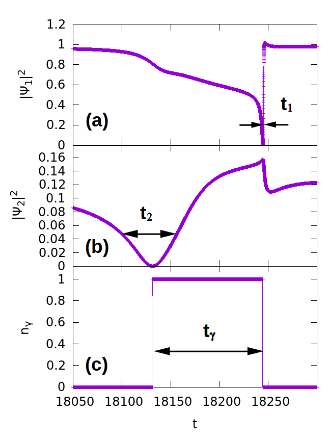
Figure 6: Structure of a t-PS. Time dependence of (a) $|\Psi_{1}|^{2}$, (b) $|\Psi_{2}|^{2}$ and (c) $\nu_{\gamma}$, at $x=L/2=25\xi_{1}$ for $J=0.372$ . For this current density, $\nu_{\gamma}(L/2,t)=n_{\gamma}(t)$. Time is normalized by $t_{0}$ and order parameters by $\Psi_{10}^{2}$.

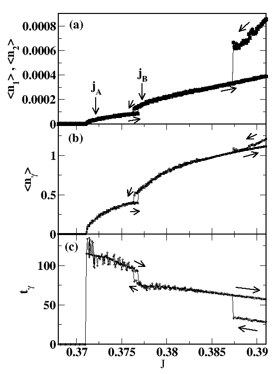
Figure 7: (a) Average number of phase slips in each of the two bands. Square symbols represent $\langle n_{1}\rangle$ and triangles represent $\langle n_{2}\rangle$. They are difficult to distinguish in the plot since both values coincide. (b) Average number of interband time-vortices, $\langle n_{\gamma}\rangle$. (c) Estimated average time length, ${\bar{t}_{\gamma}}=\delta t\langle n_{\gamma}\rangle/\langle n_{i}\rangle$, normalized by $t_{0}$. Current $J$ is normalized by $j_{0}$.

In Fig.7 we study, as a function of $J$, the average number of phase slips per step, $\langle n_{i}\rangle=\frac{1}{N_{T}}\sum_{x,t}\nu_{i}(x,t)$ (with $N_{T}$ the number of time steps, and the time-averaged total number of interband vortices $\langle n_{\gamma}\rangle=\frac{1}{N_{T}}\sum_{x,t}\nu_{\gamma}(x,t)$. We find that, as expected, the number of PS is the same in each band, and that they agree with the average voltage, $\langle n_{1}\rangle=\langle n_{2}\rangle\sim V/2\pi$. We see in Fig.7 (b) that simultaneously with the nucleation of PS above $j_{c}$, there is a finite interband vorticity $\langle n_{\gamma}\rangle$ that increases with the current.

More interestingly, we can quantify the average time length of the t-PS. We estimate numerically the average time-length of time-vortices as ${\bar{t}_{\gamma}}=\delta t\langle n_{\gamma}\rangle/\langle n_{i}\rangle$. ($\delta t\langle n_{t}\rangle$ is total time-length of time-vortices, and ${\bar{t}_{\gamma}}$ is the time-length per t-PS). When there is only one PS center in the sample, with vorticity $1$, ${\bar{t}_{\gamma}}$ is the time-length of the t-PS. We plot in Fig.7 (c) the dependence of ${\bar{t}_{\gamma}}$ on the current. When approaching the critical current $j_{c}$ from above the length ${\bar{t}_{\gamma}}$ increases, reaching its largest value at $J\rightarrow j_{c}^{+}$. For $J<j_{c}$ there are no time-vortices and their length becomes meaningless; we adopt the convention to define ${\bar{t}_{\gamma}}=0$ whenever $\langle n_{\gamma}\rangle=0$, to emphasize the difference with the case of phase solitons tanaka2001 ; gurevich2003 , for which $\langle n_{\gamma}\rangle\not=0$ and $\langle n_{i}\rangle=0$, implying that ${\bar{t}_{\gamma}}$ is infinite.

V Dependence on interband coupling and relaxation parameters

To study the dependence of the t-PS on the interband coupling $g$, it is more convenient to work at a fixed voltage $V$ than at fixed current $J$. The current $j_{c}$ for the onset of voltage changes when changing the system parameters. If $J$ is fixed and $g$ is varied, the voltage will change with $g$ due to the dependence of $j_{c}$ with $g$. On the other hand, by fixing the voltage $V$, we are guaranteed to work at a fixed time-scale, given by the expected time period for phase slips, $\tau_{V}\propto 1/V$.

Numerically, we impose the fixed voltage $V$ by solving the second order equation for $\phi(x,t)$:

$$-\frac{\partial^{2}\phi}{\partial x^{2}}+\frac{\partial}{\partial x}\left[\operatorname{Im}\left(\Psi_{1}^{*}\nabla\Psi_{1}\right)+k\operatorname{Im}\left(\Psi_{2}^{*}\nabla\Psi_{2}\right)\right]=0\;,$$ (13)

with the boundary condition $\phi(0,t)=0$, $\phi(L,t)=-VL$. In this case the current depends on time, and it can be calculated as $J(t)=V+\frac{1}{L}\int_{0}^{L}[\operatorname{Im}\left(\Psi_{1}^{*}\nabla\Psi_{1}\right)+k\operatorname{Im}\left(\Psi_{2}^{*}\nabla\Psi_{2}\right)]dx$. Simultaneously, the TDGL equations for $\Psi_{i}(x,t)$ are solved with the superconducting bank boundary conditions, as in the previous sections.

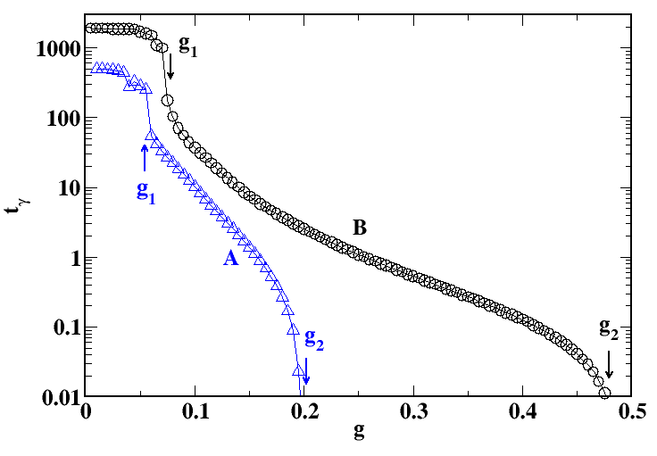
Figure 8: Estimated average time length ${\bar{t}_{\gamma}}$ (normalized by $t_{0}$) as a function of the interband coupling parameter $g=\gamma/|\alpha_{1}|$. Parameter sets A: $(V=0.00745,a=0.2,b=0.7,k=5.2,d=10,\eta_{1}=0.07)$, and B: $(V=0.002,a=0.2,b=1.2,k=5.2,d=2,\eta_{1}=0.5)$. The limits $g_{1}$ and $g_{2}$ for the existence of t-PS are indicated.

We fix a low voltage, near the onset of dissipation, and plot in Fig.8 the average time-length of the t-PS, ${\bar{t}_{\gamma}}$, as a function of the interband coupling $g$, for two different choices of parameters, both in the case $t_{2}/t_{0}=\eta_{2}/a>1$ and $t_{1}/t_{0}=\eta_{1}<1$. Ref.gurevich2003 estimated the time scale for variations in the interband phase as $t_{\rm interband}=\eta_{1}\eta_{2}\Delta_{1}\Delta_{2}/[g(\Delta_{1}^{2}\eta_{1}+\Delta_{2}^{2}\eta_{2})]$ for the case of low current, $J\ll j_{c}$ (no dissipation, $v=0$), in the limit of small coupling, $g\ll a$; $\Delta_{1}$ and $\Delta_{2}$ are the equilibrium order parameters. Fig.8 shows that ${\bar{t}_{\gamma}}$ decreases with increasing $g$, as expected from the estimate of $t_{\rm interband}$, but the dependence is more complex since, among other factors, $\Delta_{1}$ and $\Delta_{2}$ depend on $g$, and on the applied voltage.

We find that the t-PS can occur in an interval $g_{1}<g<g_{2}$. Below a coupling $g_{1}$ the value of ${\bar{t}_{\gamma}}$ saturates to a constant, while at $g_{2}$ the time ${\bar{t}_{\gamma}}$ vanishes. The lower limit $g_{1}$ corresponds to the condition that $t_{\gamma}$ has to be smaller than the period of the PS (the t-PS do not overlap), $t_{\gamma}<\tau_{V}$. The value of $g_{1}$ is reached when $t_{\gamma}\approx\tau_{V}\approx 2\pi/V$. Indeed, we find that the saturation value of ${\bar{t}_{\gamma}}$ grows as $1/V$.

The upper limit $g_{2}$ stems from requirement that $t_{\gamma}$ has to be larger than the smallest relaxation time of the order parameters, in this case $t_{\gamma}>t_{1}=\eta_{1}$. If this condition is not fulfilled, the PS of the two order parameters are effectively synchronized. Fenchenko and Yerin fenchenko2012 studied PS in two-band superconducting wires, finding synchronized PS. Indeed, the TDGL parameters studied in their work correspond to the $g>g_{2}$ case of our analysis.

We can also see in Fig.8 that for larger relaxation parameter $\eta_{1}$ (always under the condition $t_{2}>t_{1}$) the time length $t_{\gamma}$ is larger, as expected from the above mentioned expression for $t_{\rm interband}$. For $\eta_{1}>1$, however, the upper limit $g_{2}$ decreases significantly, and the region $g_{1}<g<g_{2}$ where the t-PS could be generated becomes too small.

VI Discussion

We have found a new topological object in driven one-dimensional two-band superconductors. Above the critical current we find that there are separate nucleations of PS in each band that are displaced in time and topologically connected through a vortex string oriented along the time direction. It is interesting to note that the t-PS are analogous to kinked vortices in layered superconductors feinberg1990 ; ivlev1990 ; blatter1994 (see for instance the Fig.35 of blatter1994 ). In kinked vortices there are two-dimensional space coordinates instead of space-time coordinates, and the 2D pancake vortices are the analogues of the PS. However, even though the topological structures of t-PS and kinked vortices are similar, their physics and dynamical behavior is, of course, very different.

In single-band one dimensional superconductors, the possible solutions depend on one free parameter of the TDGL equation (the relaxation rate $\eta$), plus the length of the wire $L$, the boundary conditions, and the driving current $J$ michotte2004 ; vodolazov2011 ; ludac2008 ; kim2010 ; baranov2011 ; baranov2013 ; kallush2014 ; berger2015 ; kimmel2017 . In the case of two-band superconductors, there are six free parameters in the TDGL equations ($a,b,k,g,\eta_{1},\eta_{2}$), in addition to wire length, boundary conditions and driving current $J$. Therefore, there is a large variety of behaviors one could find in this problem. Besides the parameter sets shown here, we have explored several other choices of the TDGL equation parameters comment2 within the ranges $0<a<1$, $b>a$, $k>a$, $g<a$, $\eta_{2}/a>\eta_{1}$ . (Note that after exchange of the band index $1\rightarrow 2$ in the TDGL equations, the parameters change as $a\rightarrow 1/a$ , $b\rightarrow 1/b$, $k\rightarrow 1/k$, $g\rightarrow g/a$ $\eta_{1}\rightarrow\eta_{2}ak/b$, $\eta_{2}\rightarrow\eta_{1}ak/b$, and the same results are obtained.) We have also explored two other possible boundary conditions: (i) $\partial\Psi_{i}/\partial x=0$ at $x=0,L$, and (ii) $\Psi_{i}=0$ at $x=0,L$; and system sizes in the range $L/\xi_{1}=10-250$.

We have found that the nucleation of t-PS occurs for most of the parameters explored, always within some range $g_{1}<g<g_{2}$, and in a narrow range of currents near a critical current $j_{c}$. The range in $g$ depends on the parameters $a,b,k,\eta_{1},\eta_{2}$ and the voltage $V$, as shown in Fig.8 for two particular cases. The occurrence of t-PS is independent of the boundary conditions, i.e. it is a bulk phenomenon. Different boundary conditions give slightly different history dependencies in the current-voltage curve, but in all cases there are t-PS above an onset current $j_{c}$.

When decreasing the current, approaching the critical current from above, the time length $t_{\gamma}$ increases. One could think that when $J\rightarrow j_{c}^{+}$, $t_{\gamma}\rightarrow\infty$. Even though we do not discard this scenario, we do not find such a divergence for the range of currents explored. Another related question is if there is a relationship between the existence of the t-PS for $J>j_{c}$ and the existence of phase solitons for $J<j_{c}$. In principle, a t-PS with $t_{\gamma}=\infty$ is a phase soliton, i.e., there is a phase texture with $\theta_{1}\neq\theta_{2}$ at a given point in space for all times gurevich2003 ; gurevich2006 ; tanaka2001 . Or one could interpret the periodic sequence of t-PS as a ‘dismembered’ phase soliton which is interrupted by PS and broken in several segments along the time direction. We have found that for some sets of TDGL parameters it is possible to have both, phase solitons for $J<j_{c}$ and t-PS for $J>j_{c}$, but this is not always the case. In general, there is no direct connection between the conditions for the existence of these two topological objects. For the two sets of TDGL parameters shown in this paper there are no phase solitons for $J<j_{c}$, and there are t-PS above $j_{c}$.

For increasing current, there are jumps to different dynamical regimes in the current-voltage curve, as seen for instance in Fig.1. At first, we find regimes with one, two, three t-PS centers. The maximum number of t-PS centers obtained depends on the length $L$. At larger currents other dynamical regimes are found: quasiperiodic regimes with two or more t-PS centers each with different periodicity, chaotic regimes (similar to what was reported in fenchenko2012 ), a regime where in one part of the wire the 2-band is normal, and on top of it there are PS of the 1-band, with the size of the 2-band normal sector growing with current, etc. Which of these high-current regimes are observed, depends on the choices of the TDGL parameter sets. Here we have focused on describing the t-PS and their topological structure, and leave for future work the study of the very rich variety of dynamical behaviors that can be found in current driven two-band superconducting wires.

A possible experimental evidence of t-PS would be the measurement of a two-peak structure in the time dependence of the voltage near the critical current. This requires a resolution in the time scale of $t_{\gamma}\sim 10-100t_{0}$. Since $t_{0}\sim 10^{-11}-10^{-10}s$ in conventional superconductors kadin1986 , this can be very challenging to achieve. Besides two-band superconductors like MgB₂ and iron compounds, the t-PS can also be observed in artificially fabricated structures of Josephson-coupled bilayer superconductors bluhm2006 ; ishizu2023 , where parameters could be tuned by using layers with different mean free path, or layers with different superconductors, or varying the layer and interlayer thicknesses.

Acknowlegments

DD acknowledges support from CNEA, CONICET , ANPCyT ( PICT2019-0654) and UNCuyo (06/C026-T1).

Appendix A Crank-Nicholson algorithm for the two-band TDGL equations

To solve the TDGL equations we adapt to the one-dimensional two-component superconductor the semi-implicit Cranck-Nicholson algorithm described in winiecki2002 .

In the $x$ coordinate we use the discretization,

$$\frac{\partial^{2}\Psi(x,t)}{\partial x^{2}}\rightarrow\frac{\Psi(x+dx,t)+\Psi(x-dx,t)-2\Psi(x,t)}{dx^{2}}$$

For a one-component superconductor, the Crank-Nicholson method discretizes the time dependence of the equation

$$\left(\frac{\partial}{\partial t}+i\phi\right)\Psi(x,t)=D(x,t)$$

as:

$$\frac{\Psi(x,t+dt)-e^{-i\phi dt}\Psi(x,t)}{dt}=\frac{1}{2}[D(x,t)+D(x,t+dt)]$$

with

$$D(x,t)=\frac{1}{\eta}\left(\frac{\partial^{2}\Psi(x,t)}{\partial x^{2}}+(1-|\Psi(x,t)|^{2}\right)$$

and $dt$ is the time step discretization.

In the nonlinear term of $D(x,t+dt)$ we approximate $|\Psi(x,t+dt)|^{2}\approx|\Psi(x,t)|^{2}$. In this way, it is possible to rewrite the equations to obtain $\Psi(x,t+dt)$ as a function $\Psi(x,t)$ solving the tridiagonal form,

$$A_{n}\Psi_{n}(t+dt)+B\Psi_{n+1}(t+dt)+B\Psi_{n-1}(t+dt)$$

$$=f_{n}(t)$$ (14)

with the coefficients $A_{n}=1+\frac{dt}{2\eta}(\frac{2}{dx^{2}}-1+|\Psi_{n}(t)|^{2})$ and $B=-\frac{dt}{2\eta dx^{2}}$. The right hand side term is $f_{n}(t)=\Psi_{n}(t)e^{-i\phi_{n}(t)dt}+\frac{dt}{2}D_{n}(t)$. The subindex $n$ indicates the discretized spatial coordinate, $\Psi_{n}(t)=\Psi(ndx,t)$. For a systen of length $L$, we define $N$ as $dxN=L$. We solve the tridiagonal equation with the recurrence:

$$\Psi_{n-1}(t+dt)=\alpha_{n}\Psi_{n}(t+dt)+\beta_{n}$$

where

$$\alpha_{n+1} = -\frac{B}{B\alpha_{n}+A_{n}}$$ (15)

$$\beta_{n+1} = \alpha_{n+1}(\beta_{n}-\frac{f_{n}}{B})$$ (16)

In the case of Dirichlet boundary conditions that fix $\Psi(x=0)=\Psi_{0}$ and $\Psi(x=L)=\Psi_{N}$, the recurrence equations for $\alpha_{n}$ and $\beta_{n}$ are started with $\alpha_{1}=0$, $\beta_{1}=\Psi_{0}$. Once obtained $\alpha_{n}$ and $\beta_{n}$, the recurrence equation for $\Psi_{n}$ is started from $n=N$ with the boundary value $\Psi_{N}$.

In the two-band case, the Crank-Nicholson method leads to two coupled tridiagonal equations casali2013 ,

$$A_{1,n}\Psi_{1,n}+B_{1}\Psi_{1,n+1}+B_{1}\Psi_{1,n-1}+C_{1}\Psi_{2,n}=f_{1,n}(t)$$

$$A_{2,n}\Psi_{2,n}+B_{2}\Psi_{2,n+1}+B_{2}\Psi_{2,n-1}+C_{2}\Psi_{1,n}=f_{2,n}(t)$$

with $\Psi_{1,n}$, $\Psi_{2,n}$ in the left hand side evaluated at $t+dt$. The coefficients are $A_{1,n}=1+\frac{dt}{2\eta_{1}}\left(\frac{2}{dx^{2}}-1+|\Psi_{1,n}(t)|^{2}\right)$, $A_{2,n}=1+\frac{dt}{2\eta_{2}}\left(\frac{2k}{dx^{2}}-a+b|\Psi_{2,n}(t)|^{2}\right)$, $B_{1}=-\frac{dt}{2\eta_{1}dx^{2}}$, $B_{2}=-\frac{kdt}{2\eta_{2}dx^{2}}$, $C_{1}=-\frac{dt}{2\eta_{1}}g$, $C_{2}=-\frac{dt}{2\eta_{2}}g$. The right-hand side terms are $f_{i,n}(t)=\Psi_{i,n}(t)e^{-i\phi_{n}(t)dt}+\frac{dt}{2}D_{i,n}(t)$; with $D_{1}(x,t)=\frac{1}{\eta_{1}}\left(\frac{\partial^{2}\Psi_{1}(x,t)}{\partial x^{2}}+(1-|\Psi_{1}(x,t)|^{2}\right)$, and $D_{2}(x,t)=\frac{1}{\eta_{2}}\left(k\frac{\partial^{2}\Psi_{2}(x,t)}{\partial x^{2}}+(a-b|\Psi_{2}(x,t)|^{2}\right)$.

The recurrences are

$$\Psi_{1,n-1}=\alpha_{1,n}\Psi_{1,n}+\beta_{1,n}+\delta_{1,n}\Psi_{2,n}$$

$$\Psi_{2,n-1}=\alpha_{2,n}\Psi_{2,n}+\beta_{2,n}+\delta_{2,n}\Psi_{1,n}$$

with

$$\alpha_{1,n+1}=-\frac{B_{1}}{h_{n}}(A_{2,n}+B_{2}\alpha_{2,n})$$

$$\alpha_{2,n+1}=-\frac{B_{2}}{h_{n}}(A_{1,n}+B_{1}\alpha_{1,n})$$

$$\delta_{1,n+1}=\frac{B_{2}}{h_{n}}(C_{1}+B_{1}\delta_{1,n})$$

$$\delta_{2,n+1}=\frac{B_{1}}{h_{n}}(C_{2}+B_{2}\delta_{2,n})$$

$$\beta_{1,n+1}=\alpha_{1,n+1}(\beta_{1,n}-\frac{f_{1,n}}{B_{1}})+\delta_{1,n+1}(\beta_{2,n}-\frac{f_{2,n}}{B_{2}})$$

$$\beta_{2,n+1}=\alpha_{2,n+1}(\beta_{2,n}-\frac{f_{2,n}}{B_{2}})+\delta_{2,n+1}(\beta_{1,n}-\frac{f_{1,n}}{B_{1}})\;,$$

with $h_{n}=(A_{1,n}+B_{1}\alpha_{1,n})(A_{2,n}+B_{2}\alpha_{2,n})-(C_{1}+B_{1}\delta_{1,n})(C_{2}+B_{2}\delta_{2,n})$. For the boundary conditions that fix $\Psi_{i}(x=0)=\Psi_{i,0}$ and $\Psi_{i}(x=L)=\Psi_{i,N}$, the recurrence equations for the $\alpha$’s, $\beta$’s and $\delta$’s are started with $\alpha_{1,1}=\alpha_{2,1}=\delta_{1,1}=\delta_{2,1}=0$, $\beta_{i,1}=\Psi_{i,0}$. Once obtained the $\alpha$’s, $\beta$’s and $\delta$’s, the recurrence equations for $\Psi_{i,n}$ are started from $n=N$ with the boundary values $\Psi_{i,N}$.

Standard Euler and Runge-Kutta algorithms require small $dt$ integration steps for stability, since the TDGL equations are of diffusion type. In our case, we need a $dt\sim 0.001$ to achieve stability in an Euler algorithm. The advantage of the Crank-Nicholson algorithm is its stability for large time steps winiecki2002 . In our case we have verified that for up to $dt=0.5$ we can have numerically stable solutions. Here we solve the TDGL equations with $dt=0.02$ for better accuracy. In our simulations we have integrated the equations allowing for equilibration for each value of $J$ (or $V$ in the fixed voltage case) in the first $10^{6}$ time steps, and time averages are computed for the following $10^{5}$ steps.

Appendix B Gauge-invariant formulation of PS vorticity

The Eq.(6) has to be rewritten in a gauge invariant form, to properly take into account electric potential variations ivlev1978 . Defining the gauge invariant space-time vectors

$${\vec{q}}_{i}=(\frac{\partial\theta_{i}}{\partial x}-\frac{2e}{\hbar c}A_{x},\frac{\partial\theta_{i}}{\partial t}+\frac{2e}{\hbar}\phi),$$

we obtain the Ivlev and Kopnin result ivlev1978 in its complete form, and generalized for multiband superconductors, as

$$\oint{\vec{q}}_{i}\cdot d{\vec{\rho}}={2\pi}\nu_{i}-\frac{2e}{\hbar}\int_{S}E\cdot d\sigma,$$

where $E$ is the electric field and the integral $\int_{S}$ is in the space-time surface enclosed by the loop, with $d\sigma=dxdt$. This is valid for any space-time loop. For a large loop that extends of for a long total time $T$ and along the whole length $L$ of the wire we can consider that the left-hand side vanishes, and we obtain the quantization condition ivlev1978

$${2\pi}N_{i}=\frac{2e}{\hbar}\langle E\rangle LT\,,$$

where $N_{i}$ is the total number of PS in the $i$-band in the time interval $T$, and $\langle E\rangle$ is the space-time averaged electric field. Therefore, the average electric field is proportional to the average number of PS per unit time, $\langle n_{i}\rangle=N_{i}/T$. Since the expression at the right of equality is the same for both bands, we deduce that there must be the same total number of PS in the two bands, ${\it i.e.}$, $N_{1}=N_{2}$.

For an infinitesimal loop along the discretization distances $dx,dt$ [as shown in Fig.4(a)], we define the gauge-invariant space and time discrete phase differences as

$$\delta_{x}\theta_{i}(x,t) = \theta_{i}(x+dx,t)-\theta_{i}(x,t)-A_{x}(x,t)$$

$$\delta_{t}\theta_{i}(x,t) = \theta_{i}(x,t+dt)-\theta_{i}(x,t)+\phi(x,t)dt.$$

Then, to calculate numerically the local vorticities in the standard way teitel1993 ; phillips2015 ; smorgrav2005 , redefining each of the local gauge invariant differences in the $(-\pi,\pi)$ interval we obtain:

$$2\pi\nu_{i}(\tilde{x},\tilde{t}) = [\delta_{x}\theta_{i}(x,t)]+[\delta_{t}\theta_{i}(x+dx,t)]-$$

$$[\delta_{x}\theta_{i}(x,t+dt)]-[\delta_{t}\theta_{i}(x,t)]+$$

$$\left(\phi(x,t)-\phi(x+dx,t)\right)dt$$

where, for a phase $\alpha$, $[\alpha]$ is taken in the interval $(-\pi,\pi)$, numerically calculated as $[\alpha]=\alpha-2\pi{\rm nint}(\frac{\alpha}{2\pi})$, with ${\rm nint}(u)$ the nearest integer of $u$. The last term corresponds to the local electric field $\phi(x,t)-\phi(x+dx,t)=E(x,t)dx$, and the point ($\tilde{x},\tilde{t}$) is located in the interior of the considered plaquete. In terms of the link integers, the expression (7) stays the same

$$\nu_{i}(\tilde{x},\tilde{t}) = m_{i,x}(x,t)+m_{i,t}(x+dx,t)$$ (18)

$$-m_{i,x}(x,t+dt)-m_{i,t}(x,t)\,.$$

The link integers in their gauge invariant form are

$$m_{i,x}(x,t) = -{\rm nint}\left(\frac{\theta_{i}(x+dx,t)-\theta_{i}(x,t)-A_{x}(x,t)}{2\pi}\right)$$

$$m_{i,t}(x,t) = -{\rm nint}\left(\frac{\theta_{i}(x,t+dt)-\theta_{i}(x,t)+\phi(x,t)dt}{2\pi}\right)$$

In this work, we have calculated numerically the vorticities using the above expressions in the gauge with $A_{x}=0$.

References

- (1) A. A. Abrikosov, Zh. Eksp. Teor. Fiz. 32, 1442 (1957) [Sov. Phys. JETP, 5, 1174 (1957)].
- (2) M. Tinkham, Introduction to Superconductivity, 2nd ed. (McGraw-Hill, Inc., New York, 1996).
- (3) W. J. Skocpol, M. R. Beasley, and M. Tinkham, J. Low Temp. Phys. 16, 145 (1974).
- (4) L. Kramer and A. Baratoff, Phys. Rev. Lett. 38, 518 (1977).
- (5) B. I. Ivlev and N. B. Kopnin, Pis’ma ZhETF 28, 640 (1978) [Sov.Phys. JETP Lett. 28, 592 (1978)].
- (6) L. Kramer and R. J. Watts-Tobin, Phys. Rev. Lett. 40, 1041 (1978).
- (7) B. I. Ivlev, N. B. Kopnin, and L. A. Maslova, Zh. Eksp. Teor. Fiz. 78, 1963 (1980) [Sov. Phys. JETP 51, 986 (1980)]; B. I. Ivlev, N. B. Kopnin, and I. A. Larkin, Zh. Eksp. Teor. Fiz. 88, 575 (1985) [Sov. Phys. JETP 61, 337 (1985)].
- (8) R. J. Watts-Tobin, Y. Krahenbuhl, and L. Kramer, J. Low Temp. Phys. 42, 459 (1981).
- (9) B. I. Ivlev and N. B. Kopnin, Usp. Fiz. Nauk 142 , 435 (1984) [Sov. Phys. Usp. 27 , 206 (1984)].
- (10) N. Kopnin, Theory of Nonequilibrium Superconductivity (Oxford University Press, New York, 2001).
- (11) S. Michotte, S. Mátéfi-Tempfli, L. Piraux, D. Y. Vodolazov, and F. M. Peeters, Phys. Rev. B 69, 094512 (2004).
- (12) Mathieu Lu-Dac and V. V. Kabanov, Phys. Rev. B 79, 184521 (2009).
- (13) J. Kim, J. Rubinstein, and P. Sternsberg, Physica C 470, 630 (2010).
- (14) D. Yu. Vodolazov and F. M. Peeters, Phys. Rev. B 84, 094511 (2011).
- (15) V. V. Baranov, A. G. Balanov, and V. V. Kabanov, Phys. Rev B 84, 094527 (2011).
- (16) V. V. Baranov, A. G. Balanov, and V. V. Kabanov, Phys. Rev. B 87, 174516 (2013).
- (17) Shimshon Kallush and Jorge Berger, Phys. Rev. B 89, 214509 (2014).
- (18) J. Berger, Rev. B 92, 064513 (2015).
- (19) Gregory Kimmel, Andreas Glatz,and Igor S. Aranson, Phys. Rev. B 95, 014518 (2017).
- (20) Jože Buh, Viktor Kabanov, Vladimir Baranov, Aleš Mrzel, Andrej Kovič and Dragan Mihailovic, Nature Communications 6, 10250 (2015).
- (21) Ivan Madan, Jože Buh, Vladimir Baranov, Viktor Kabanov, Aleš Mrzel, and Dragan Mihailovic, Sci. Adv.4 , eaao0043 (2018).
- (22) Kota Kato, Tasuku Takagi, Takasumi Tanabe, Satoshi Moriyama, Yoshifumi Morita and Hideyuki Maki, Scientific Reports 10, 14278 (2020).
- (23) H. J. Choi, D. Roundy, H. Sun, M. L. Cohen and S. G. Louie, Nature, 418, 758 (2002).
- (24) E. Boaknin, M. A. Tanatar, J. Paglione, D. Hawthorn, F. Ronning, R. W. Hill, M. Sutherland, L. Taillefer, J. Sonier, S. M. Hayden, and J. W. Brill, Phys. Rev. Lett. 90, 117003 (2003).
- (25) Y. Singh, C. Martin, S. L. Budko, A. Ellern, R. Prozorov, and D. C. Johnston, Phys. Rev. B 82, 144532 (2010).
- (26) R. Khasanov, M. Bendele, A. Amato, K. Conder, H. Keller, H.-H. Klauss, H. Luetkens, and E. Pomjakushina, Phys. Rev. Lett. 104, 087004 (2010).
- (27) H. Kim, M. A. Tanatar, Y. J. Song, Y. S. Kwon, and R. Prozorov, Phys. Rev. B 83, 100502 (2011).
- (28) E. Babaev, Phys. Rev. Lett. 89, 067001 (2002).
- (29) E. Smørgrav, J. Smiseth, E. Babaev, and A. Sudbø, Phys. Rev. Lett. 94, 096401 (2005).
- (30) L. F. Chibotaru, V. H. Dao, and A. Ceulemans, Europhys. Lett. 78, 47001 (2007); L. F. Chibotaru and V. H. Dao, Phys. Rev. B 81, 020502(R) (2010).
- (31) R. Geurts, M. V. Milošević, and F. M. Peeters, Phys. Rev. B 81, 214514 (2010).
- (32) J. C. Piña, C. C. de Souza Silva, and M. V. Milošević, Phys. Rev. B 86, 024512 (2012).
- (33) R. M. da Silva, M. V. Milošević, D. Domínguez, F. M. Peeters, and J. Albino Aguiar, Appl. Phys. Lett. 105, 232601 (2014).
- (34) M. A. Silaev, Phys. Rev. B 83, 144519 (2011).
- (35) S.-Z. Lin and L. N. Bulaevskii, Phys. Rev. Lett. 110, 087003 (2013).
- (36) A. S. Mosquera Polo, R. M. da Silva, A. Vagov, A. A. Shanenko, C. E. Deluque Toro, and J. Albino Aguiar, Phys. Rev. B 96, 054517 (2017).
- (37) Y. Tanaka, Phys. Rev. Lett. 88, 017002 (2001).
- (38) A. Gurevich and V.M. Vinokur, Phys. Rev. Lett. 90, 047004 (2003).
- (39) A. Gurevich and V.M. Vinokur, Phys. Rev. Lett. 97, 137003 (2006).
- (40) Y.S. Yerin, A.N. Omelyanchouk, Low Temp. Phys. 33, 401 (2007).
- (41) S.-Z. Lin and X. Hu, New J. Phys. 14 , 063021 (2012)
- (42) S.-Z. Lin, J. Phys.: Condens. Matter 26 493202 (2014).
- (43) Y.Tanaka, I.Hase, T.Yanagisawa, G.Kato, T.Nishio, S.Arisawa, Physica C, 516, 10-16 (2015).
- (44) Y. Tanaka, G. Kato, T. Nishio, S. Arisawa, Solid State Commun. 201, 9597 (2015).
- (45) P. M. Marychev, and D. Yu. Vodolazov, Phys. Rev. B 97, 104505 (2018).
- (46) V.N. Fenchenko, Y.S. Yerin, Physica C 480, 129 (2012).
- (47) Jorge Berger and Milorad V. Milošević, Phys. Rev. B 84, 214515 (2011).
- (48) M.E. Zhitomirsky, V.H. Dao, Phys. Rev. B 69, 054508 (2004).
- (49) A. Gurevich, Phys. Rev. B 67, 184515 (2003).
- (50) A. E. Koshelev, A. A. Varlamov, and V. M. Vinokur, Phys. Rev. B 72, 064523 (2005).
- (51) A. Vargunin, M. A. Silaev, and E. Babaev, Europhys. Lett. 130, 17001 (2020).
- (52) Wenqing Dai, V. Ferrando, A. V. Pogrebnyakov, R. H. T Wilke, Ke Chen, Xiaojun Weng, Joan Redwing, Chung Wung Bark, Chang-Beom Eom, Y Zhu, P M Voyles, Dwight Rickel, J B Betts, C H Mielke, A Gurevich, D C Larbalestier, Qi Li and X X Xi, Supercond. Sci. Technol. 24 , 125014 (2011).
- (53) See for instance Ying-Hong Li and S. Teitel Phys. Rev. B 47, 359 (1993); A. K. Nguyen and A. Sudbø, Phys. Rev. B 57, 3123 (1998).
- (54) Carolyn L. Phillips, Tom Peterka, Dmitry Karpeyev, and Andreas Glatz, Phys. Rev. E 91, 023311 (2015).
- (55) Viacheslav V. Dremov, Sergey Yu. Grebenchuk, Andrey G. Shishkin, Denis S. Baranov, Razmik A. Hovhannisyan, Olga V. Skryabina, Nickolay Lebedev, Igor A. Golovchanskiy, Vladimir I. Chichkov, Christophe Brun, Tristan Cren, Vladimir M. Krasnov, Alexander A. Golubov, Dimitri Roditchev and Vasily S. Stolyarov, Nature Communications 10, 4009 (2019).
- (56) We note that is also possible to define a space-oriented interband vorticity as . This corresponds to an interband vorticity in the direction perpendicular to the time-vortex line in Fig.4(b). We have found that in the regimes where there are t-PS, meaning that the PS centers in the two bands always occur in the same point in space. At higher currents, when there are chaotic regimes, or when the 2-band becomes partially or totally normal, we find that .
- (57) D. Feinberg and C. Villard, Phys. Rev. Lett. 65, 919 (1990); Mod. Phys. Lett. B 4, 9 (1990).
- (58) B. I. Ivlev, Yu. N. Ovchinnikov and V. L. Pokrovsky, Europhys. Lett. 13, 187 (1990); Mod. Phys. Lett. B 5, 73 (1991).
- (59) G. Blatter, M.V. Feigel’man, V.B. Geshkenbein, A. I. Larkin, V. M. Vinokur, Rev. Mod. Phys. 66, 1125 (1994).
- (60) The parameter sets that we have explored were within the ranges , , , , , and , in different combinations keeping the relations , , , .
- (61) A. M. Kadin and A. M. Goldman, in Nonequilibrium Superconductivity, edited by D. N. Langenberg and A. I. Larkin, North-Holland, Amsterdam, 1986, p. 253.
- (62) H. Bluhm, N. C. Koshnick, M. E. Huber, and K. A. Moler, Phys. Rev. Lett. 97, 237002 (2006).
- (63) Hiroshi Ishizu, Hirotake Yamamori, Shunichi Arisawa, Taichiro Nishio, Kazuyasu Tokiwa, and Yasumoto Tanaka, Physica C 605, 1354208 (2023).
- (64) T. Winiecki and C. S. Adams, J. Comp. Phys. 179, 127 (2002).
- (65) P. Casali, Licenciado Thesis, Instituto Balseiro (2013).