Thermoelectric and viscous contributions to the hydrodynamic ratchet effect

Abstract

We study thermoelectric and viscous contributions to the ratchet effect, i.e. radiation-induced generation of the direct electric current, $J_{\rm rat},$ in asymmetric dual-grating gate structure without inversion center. Previously [E.Mönch et al, Phys. Rev. B 105, 045404 (2022)], it was demonstrated that frequency dependence of the $J_{\rm rat}$ is essentially different within hydrodynamic (HD) and drift-diffusion (DD) regimes of the electron transport: $J_{\rm rat}^{\rm HD}\propto 1/\omega^{6}$ and $J_{\rm rat}^{\rm DD}\propto 1/\omega^{2}$ for $\omega\to\infty.$ Here we analyze previously neglected thermoelectric contribution and find that it yields high-frequency asymptotic $1/\omega^{2}$ even in the HD regime and can change sign of the response. Account of the finite viscosity of the electron liquid yields contribution which scales at high frequency as $1/\omega^{4}.$ We also find plasmonic resonances in the $J_{\rm rat},$ and demonstrate that asymmetry of the structure allows for excitation of the so-called directional travelling plasmons.

I Introduction

One of the most general and fascinating phenomena in optoelectronics is the ratchet effect—the generation of a dc electric current in response to an ac electric field in systems with broken inversion symmetry (for reviews see, e.g., Refs. Linke (2002); Reimann (2002); Hänggi and Marchesoni (2009); Ivchenko and Ganichev (2011); Denisov et al. (2014); Cubero and Renzoni (2016); Budkin et al. (2016); Reichhardt and Reichhardt (2017); Ganichev et al. (2017)). In particular, this general definition can be used for artificial structures aimed to modulate periodically the electron density in the 2D channel: long periodic grating gate structures with an asymmetric configuration of gate electrodes, e.g., dual-grating top gate (DGG) structures Olbrich et al. (2011); Otsuji et al. (2013); Boubanga-Tombet et al. (2014); Faltermeier et al. (2015); Olbrich et al. (2016). The ratchet effect was treated theoretically and observed experimentally in various low dimensional structures Olbrich et al. (2011); Otsuji et al. (2013); Boubanga-Tombet et al. (2014); Faltermeier et al. (2015); Olbrich et al. (2016); Faltermeier et al. (2017); Olbrich et al. (2009); Popov et al. (2011); Kannan et al. (2011); Nalitov et al. (2012); Kannan et al. (2012); Kurita et al. (2014); Rozhansky et al. (2015); Bellucci et al. (2016); Fateev et al. (2017); Faltermeier et al. (2018); Rupper et al. (2018); Yu (2018); Hubmann et al. (2020); Delgado-Notario et al. (2020); Sai et al. (2021); Yahniuk and et al. (2024); Hild and et al. (2024), so that the ratchet current measurements can already be considered as a standard measurement tool. It has recently been shown that the ratchet effect can also be used to observe the transition of an electron system into hydrodynamic (HD) regime. Specifically, it was demonstrated in Ref. Mönch et al. (2022), both theoretically and experimentally, that the dc response of a DGG, based on bilayer graphene, has very strikingly different frequency dependencies: $1/\omega^{6}$ in the HD regime and $1/\omega^{2}$ within the so-called drift-diffusion (DD) approximation. An analytical formula which describes the transition between both regimes was derived which was in a good agreement with obtained experimental data. The key statement of this work, namely, HD-like behavior for liquid helium temperature was also confirmed by publication Mönch et al. (2023) focused on measurement of ratchet current in the Shubnikov de Haas regime. As was argued in Ref. Mönch et al. (2023), the experimentally observed strong suppression of the second harmonic of the cyclotron resonance indicates presence of fast electron-electron collisions that drive the electron system into HD regime.

The results obtained in Refs. Mönch et al. (2022, 2023) open a wide avenue for search of the HD regime in the optical experiments. This problem has a long history and now the electronic fluid dynamics is one of the extremely actively developing areas of condensed matter physics (for review, see, e.g., Refs. Narozhny et al. (2017); Lucas and Fong (2018); Narozhny (2019); Polini and Geim (2020)). Although the pioneering works Gurzhi (1963, 1965, 1968); de Jong and Molenkamp (1995) on hydrodynamic electron and phonon transport have been done a very long time ago, the topic did not generate much interest until recently. The interest on hydrodynamic transport was triggered by the fabrication of ultraclean ballistic structures, primarily based on one-dimensional and two-dimensional carbon materials. Convincing manifestations of hydrodynamic behavior in the different transport regimes have been demonstrated in a number of recent experiments  Bandurin et al. (2016); Crossno et al. (2016); Moll et al. (2016); Ghahari et al. (2016); Kumar et al. (2017); Bandurin et al. (2018); Braem et al. (2018); Jaoui et al. (2018); Gooth and Kumar (2018); Berdyugin et al. (2019); Gallagher et al. (2019); Sulpizio et al. (2019); Ella et al. (2019); Ku et al. (2020); Raichev et al. (2020); Gusev et al. (2020); Geurs et al. (2020); Kim et al. (2020); Vool et al. (2020); Gupta et al. (2021); Gusev et al. (2021); Zhang and Shur (2021); Jaoui et al. (2021). Moreover, literally in recent years, it has been possible to experimentally visualize the hydrodynamic flow in ballistic 2D systems by using various nanoimaging techniques Braem et al. (2018); Sulpizio et al. (2019); Ella et al. (2019); Ku et al. (2020); Vool et al. (2020).

All previous publications searching the HD regime were focused on measurements of dc viscous transport. However, the approach based on optical experiments has a number of advantages. Indeed, one of the hallmarks of the viscous dc flow is the Gurzhi effect predicted in Refs. Gurzhi (1963, 1965, 1968). Starting from its first experimental observation in Ref. de Jong and Molenkamp (1995), this effect is considered as one of the most convincing arguments in favor of viscous transport. The Gurzhi effect is observed in a system of finite transverse (with respect to electron flow) width $d$ under the assumptions $l_{\rm ee}\ll d\ll L_{\rm G},$ where $l_{\rm ee}$ is the electron-electron collision length, $L_{\rm G}=\sqrt{ll_{\rm ee}}$ is the so called Gurzhi length, and $l$ is the momentum relaxation length limited by impurity and phonon scattering. The inequality $d\ll L_{\rm G}$ is not easy to satisfy in a sufficiently wide sample. That is why for the observation of viscous transport it is necessary to use narrow-channel samples with ultrahigh mobility. Also, for the observation of negative non-local resistance, see Ref. Bandurin et al. (2016), the size of the viscosity-induced whirlpools responsible for viscous back flow (this size is in the order of $L_{\rm G}$) was in the order of the size between contacts probing a negative voltage drop. If one uses thin wires or narrow strips for the observation of the Gurzhi effect, the second inequality, $l_{\rm ee}\ll d$ can be satisfied only at sufficiently high temperatures. By contrast, in the optical experiments one can study a bulk effects which do not disappear with increasing system size and distance between contacts. For the observation of the HD transport, one only need the condition $l_{\rm ee}\ll l,$ which is independent of the system size.

Moreover, the HD regime is not necessarily viscous. The key property of the HD regime (as compared to the DD one) is the presence of only three collective variables (local temperature, concentration and drift velocity), which completely characterize the system, in contrast to the DD regime, where the distribution function is not reduced to a hydrodynamic ansatz depending, in the general case, on an infinite number of variables. Hence, HD regime can be realized for the case when the viscous contribution to the resistivity is small:

$$\eta q^{2}\ll\gamma,$$ (1)

where $\eta=v_{\rm F}^{2}\tau_{\rm ee}/4$ is the electron viscosity, $\gamma=v_{\rm F}/l=1/\tau,$ $\tau$ is the momentum relaxation time, and $q$ is the characteristic inverse scale of the inhomogeneity of the problem (inequality (1) is equivalent to condition $qL_{\rm G}\ll 1$). It is worth also noting, that the latter condition is always satisfied in the limit of the ideal liquid, $\tau_{\rm ee}=0.$

On the other hand, an additional possibility to observe the HD regime appears in the non-linear excitation regime discussed in Refs. Mönch et al. (2022, 2023). In such a regime, in contrast to the linear one, the difference between the distribution functions in the DD and the HD regimes is very strong and causes currents, which are strongly different even if one neglects viscosity. This allows one to distinguish between the DD and the HD regimes even when the condition Eq. (1) is satisfied. In particular, this condition was assumed to be satisfied in Ref. Mönch et al. (2022, 2023), where the viscosity contribution was neglected.

In this paper, we focus on the thermoelectric contribution to $J_{\rm rat}$ and also take into account effect of finite viscosity still assuming that condition Eq. (1) is satisfied. Thermoelectric contribution was neglected in Ref. Mönch et al. (2022) by assuming that (see discussion in Ref. Nalitov et al. (2012))

$$\Gamma=\frac{\tau}{\tau_{\rm T}}=\frac{3\tau}{\pi^{2}\tau_{\rm ph}}\frac{\mu}{T}\gg 1,$$ (2)

where $T$ is the temperature, $\tau_{\rm T}=\tau_{\rm ph}\mathcal{C}/N=\pi^{2}T\tau_{\rm ph}/(3\mu)$ is the temperature relaxation time, $\mathcal{C}=\nu T\pi^{2}/3$ and $\nu$ are, respectively, the heat capacitance and density of states of the 2D Fermi gas, $\mu$ is the Fermi energy, and $\tau_{\rm ph}$ is the phonon scattering rate. We demonstrate that previously neglected thermoelectric contribution yields high-frequency asymptotic $1/\omega^{2}$ even in the deep HD regime ($\tau_{\rm ee}=0$) and can change sign of the response with decreasing $\Gamma$. Account of the finite viscosity of the electrton liquid yields contribution scaling at large frequency as $1/\omega^{4}.$ We also find plasmonic resonances in $J_{\rm rat},$ and demonstrate that asymmetry of the structure allows for excitation of the so-called directional plasmons. The obtained results are used to analyze conditions needed for realization of the HD regime in the optical experiments.

II Model and basic equations

The purpose of the current work is to calculate a contribution of thermoelectric effects into the ratchet current and also to take into account effects related to finite viscosity.

We will focus on the ratchet effect in 2D electron gas with a parabolic energy spectrum which is covered by a long periodic (with a period $L$) grating gate with an asymmetric configuration of gate electrodes, e.g., dual-grating top gate (DGG) structures Olbrich et al. (2011); Otsuji et al. (2013); Boubanga-Tombet et al. (2014); Faltermeier et al. (2015); Olbrich et al. (2016). Application of the voltages to the grating electrodes leads to the static periodic potential in the 2D gas,

$$U(x)=U_{0}\cos(qx+\phi),$$ (3)

which modulates the electron density in the channel. Here $q={2\pi}/{L}$ is the modulation wave-vector.

The system is illuminated by an external radiation with a large wavelength, $\lambda\gg L,$ which is linearly polarized in $x$ direction. The grating leads to modulation of this field with the depth $h.$ In particular, for linear polarization of the incoming radiation along the $x$ axis, the field, $\mathbf{E}(x,t)=E(x,t)\mathbf{e}_{x}$ ($\mathbf{e}_{x}$ is the unit vector in the $x$ direction), acting in the 2D channel, has spatially modulated amplitude:

$$E(x,t)=[1+h\cos(qx)]E_{0}\cos\omega t.$$ (4)

We assume below that $h\ll 1.$ Following Ref. Ivchenko and Ganichev (2011), we take into account the asymmetry of the structure phenomenologically, by introducing the phase shift $\phi$ between the static potential and radiation modulations.

The response of the 2D electron system to the above described perturbation can be found by using two approaches – hydrodynamic and drift-diffusion. In both approaches, the direction of the radiation-induced dc current is controlled by the lateral asymmetry parameter Ivchenko and Ganichev (2011)

$$\Xi=\left\langle|\mathbf{E}(x,t)|^{2}{\mathrm{d}U(x)\over\mathrm{d}x}\right\rangle_{t,x}=\frac{E_{0}^{2}hU_{0}q\sin\phi}{2},$$ (5)

where averaging is taken over the period $2\pi/\omega$ and distance $L.$

Actually, the effect of the ee-interaction is twofold and can be quite strong. First of all, as we mentioned, suciently fast ee-collisions can drive the system into the hydrodynamic regime. Secondly, ee-interaction leads to plasmonic oscillations, so that a new frequency scale, the plasma frequency, $\omega_{p}(q)$ appears in the problem. The ratchet effect is dramatically enhanced in the vicinity of plasmonic resonances. We start with a system of hydrodynamic equations,

$$\frac{\partial N}{\partial t}+\frac{\partial}{\partial x}\left(Nv\right)=0,$$ (6)

$$\frac{\partial v}{\partial t}+v\frac{\partial v}{\partial x}+\frac{v}{\tau}-\eta\frac{\partial^{2}v}{\partial^{2}x}={a}-s_{0}^{2}\frac{\partial n}{\partial x}-\frac{1}{mN}\frac{\partial W}{\partial x},$$ (7)

$$\mathcal{C}\left[\frac{\partial T}{\partial t}+\frac{(T{v})}{\partial x}\right]=N\left(\frac{T_{0}-T}{\tau_{ph}}+\frac{mv^{2}}{\tau}\right),$$ (8)

describing evolution of three local variables: concentration, $N=N(x,t),$ electron fluid velocity $v=v(x,t),$ and temperature $T=T(x,t).$ Here $T_{0}$ is the lattice temperature,

$$a=\frac{e}{m}\left(E-\frac{\partial U}{\partial x}\right)$$

is the total force acting on electron from both the static potential and radiation field, $s_{0}=\sqrt{eU_{\rm g}/m}$ is the plasma wave velocity, which is controlled by the backgate voltage $U_{\rm g},$ $n=(N-N_{0})/N_{0}$ is the dimensionless concentration, $N_{0}$ is the equilibrium electron concentration in 2D channel, $\eta$ is the electron viscosity, and $W$ is the local energy of the Fermi gas in the moving frame,

$$W=\nu\int\varepsilon\left[e^{(\varepsilon-\mu)/T+1}\right]^{-1}d\varepsilon\approx\frac{N^{2}}{2\nu}+\frac{\nu T^{2}\pi^{2}}{6},$$ (9)

where we took into account that for 2D gas the local concentration is connected with local chemical potential, $\mu,$ as follows: $N=\nu\mu.$ Equation (7) contains also viscous friction $\eta\partial^{2}v/\partial^{2}x$ (we neglected here a concentration dependence of this term), where $\eta$ is viscosity.

Calculating the spatial derivative of the first term in $W,$ substituting it into Eq. (7) and combining with the term $s_{0}^{2}\partial n/\partial x$, we find correction to the plasma wave velocity due to pressure of the electron liquid:

$$s_{0}\to s=\sqrt{s_{0}^{2}+v_{\rm F}^{2}/2,}$$ (10)

where $v_{\rm F}$ is the Fermi velocity. Next, calculating spatial derivative of the second term in $W$ and substituting it into Eq. (7) we find the thermoelectric correction to the r.h.s. of Eq. (7)

$$a_{\rm th}=-\frac{\pi^{2}}{3m}\frac{T}{\mu}\frac{\partial T}{\partial x}=-\frac{\mathcal{C}}{mN_{0}(1+n)}\frac{\partial T}{\partial x}.$$ (11)

Due to the term (11), Eq. (8) couples with Eqs. (6) and (7). This coupling was neglected in Refs. Rozhansky et al. (2015); Mönch et al. (2022).

Following Refs. Rozhansky et al. (2015); Mönch et al. (2022), one can solve Eqs. (6), (7), and (8) perturbatively with respect to $E_{0}$ and $U_{0}.$ Non-zero radiation-induced dc current appears in the third order (second order with respect to the radiation field and the first order with respect to static potential): $j_{\rm dc}\propto\Xi,$ where $\Xi$ is given by Eq. (5).

III Calculation

Below, we calculate separately the thermoelectric and viscous contributions.

III.1 Thermoelectric contribution

III.1.1 Linear polarization

In this section, we put $\eta=0$ and discuss a simplified approach to solution of Eqs. (6)–(8). We will start with a discussion of the linear polarization and then generalize the result for the case of arbitrary polarization. First, we notice that l.h.s. and r.h.s. of Eq. (8) are proportional to $\mathcal{C}\propto T,$ and $N\propto\mu,$ respectively. Hence, one can expect that for strongly degenerated Fermi gas, $T/\mu\ll 1,$ l.h.s. of Eq. (8) can be neglected, so that temperature is fully determined by the balance between local Joule heat and phonon cooling

$$\frac{T-T_{0}}{\tau_{\rm ph}}=\frac{mv^{2}}{\tau}.$$ (12)

Expressing temperature from this equation and substituting into Eq. (7), we get a system of closed equations for $n$ and $v$:

$$\frac{\partial n}{\partial t}+\frac{\partial[(1+n)v]}{\partial x}=0,$$ (13)

$$\frac{\partial v}{\partial t}+v\frac{\partial v}{\partial{x}}\left[1+\frac{2}{\Gamma(1+n)}\right]+\frac{v}{\tau}=a-s^{2}\frac{\partial n}{\partial x}.$$ (14)

Here and in what follows we approximate $\Gamma$ by its value at $\varepsilon=\mu.$ We will search for perturbative solution of Eqs. (13) and (14) up to the third order with respect to $a$:

$$n=n^{(0,1)}+n^{(1,0)}+\cdots,\quad v=v^{(0,1)}+{v}^{(1,0)}+\cdots,$$

where the first and second indices denote an order of expansion with respect to $E_{0}$ and $U_{0}.$ This expansion aims to calculate the averaged dc current $J_{\rm rat}=({e\tau N_{0}}/{m})\left\langle(1+n)a\right\rangle_{t,x}.$ A non-zero response appears in the order $(2,1)$. The calculation can be simplified to the purturbative expansion of the second order by using a simple identity, which can be obtained by multiplying Eq. (13) with $v,$ (14) with $(1+n),$ summing thus obtained equations and averaging over $x$ and $t.$ Doing so, we get

$$J_{\rm rat}=\frac{e\tau}{m}N_{0}\left\langle n^{(1,1)}E-n^{(2,0)}\frac{\partial U}{\partial x}\right\rangle_{t,x},$$ (15)

where $U$ and $E$ are given by Eqs. (3) and (4), respectively. Hence, we only need to calculate the concentration up to the second order with respect to $a.$

The calculations are fully analogous to the ones performed in Refs Rozhansky et al. (2015) and Mönch et al. (2022), so that we delegate them into Appendix A. The result reads

$$\frac{J_{{\rm rat},x}}{J_{0}}=\frac{\Omega^{2}(1+\Omega^{2})+\Omega_{q}^{2}(\Gamma-\Omega^{2})}{\Gamma(1+\Omega^{2})(\Omega^{2}+(\Omega^{2}-\Omega_{q}^{2})^{2})},$$ (16)

where

$$J_{0}=\frac{e^{3}\tau^{3}N_{0}qh|E_{0}|^{2}U_{0}\sin\phi}{4m^{3}s^{2}}$$ (17)

and we used dimensionless variables

$$\Omega=\omega\tau,\quad\Omega_{q}=\omega_{q}\tau.$$

For $\Gamma\to\infty$ we reproduce result of Ref. Rozhansky et al. (2015). One can easily combine this equation with formula (33) of Ref. Mönch et al. (2022), where thermoelectric effects were neglected (by assuming $\Gamma\gg 1$), while the ratchet current was calculated for an arbitrary relation between $\tau_{ee}$ and $\tau.$ This yields:

$$\frac{J_{\rm{rat},x}}{J_{0}}=\frac{\Omega_{q}^{2}+\Omega^{2}\left(1+\Omega^{2}-\Omega_{q}^{2}\right)\left[\frac{1}{\Gamma}+\frac{\tau_{ee}}{2(\tau+\tau_{ee})}\right]}{(1+\Omega^{2})(\Omega^{2}+(\Omega^{2}-\Omega_{q}^{2})^{2})}.$$ (18)

Expression in the square brackets can be written as

$$\frac{1}{\Gamma}+\frac{\tau_{ee}}{2(\tau+\tau_{ee})}=\frac{\tau_{\rm T}+\tau_{*}}{\tau},$$ (19)

where $1/(2\tau_{*})=1/\tau+1/\tau_{ee}.$ As seen, there are two terms in Eq. (18) with different asymptotic behavior at $\Omega\to\infty$: first, containing $\Omega_{q}^{2}$ in the numerator, scales as $1/\Omega^{6}$, and the second, proportional to the square bracket in the numerator with $1/\Omega^{2}$ high-frequency scaling. Physically, the second term is related with the energy relaxation processes—temperature relaxation and collision-induced thermalization.

III.1.2 Arbitrary polarization

The above result can be easily generalized for the case of an arbitrary polarization of the external field described by phases $\alpha$ and $\theta$:

$$E_{x}(x,t) =[1+h\cos(qx+\phi)]E_{0}\cos\alpha\cos\omega t,$$ (20)

$$E_{y}(x,t) =[1+h\cos(qx+\phi)]E_{0}\sin\alpha\cos(\omega t+\theta).$$ (21)

These phases are related to the standard Stokes parameters as follows: $P_{\rm L1}=\cos{2\alpha},$ $P_{\rm L2}=\sin{2\alpha}\,\cos\theta,$ $P_{\rm C}=\sin{2\alpha}\,\sin\theta.$ Calculations of the current for this case are presented in Applendix A.2. The result for the $x$ component of the current modifies as follows

$$\frac{J_{{\rm rat},x}}{J_{0}} =\frac{1}{\Gamma\left(\Omega^{2}+1\right)}$$ (22)

$$+\frac{\Omega_{q}^{2}\left[1+(\Omega^{2}-\Omega_{q}^{2})/\Gamma\right]\cos^{2}\alpha}{\left(\Omega^{2}+1\right)\left[\left(\Omega^{2}-\Omega_{q}^{2}\right)^{2}+\Omega^{2}\right]}.$$

For $\alpha=0,$ we restore Eq. (16).

There is also $y$ component of the current

$$\frac{J_{{\rm rat},y}}{J_{0}}=\frac{(\Omega_{q}^{2}-\Omega^{2})P_{\rm L2}-\Omega P_{\rm C}}{2(\Omega^{2}+(\Omega^{2}-\Omega_{q}^{2})^{2})}$$ (23)

which is insensitive to the temperature relaxation and thermalization, and coincides with previously obtained result Rozhansky et al. (2015).

We notice that for $\Gamma=\infty$ we reproduce results of Ref. Rozhansky et al. (2015). We also see that in the absence of plasmonic effects, i.e. for $\Omega_{q}\to 0$, we get for the $x$ component of the current the polarization-independent (Seebeck) contribution to the ratchet effect in the non-interaction system Ivchenko and Ganichev (2011); Nalitov et al. (2012); Budkin et al. (2016):

$$\frac{J_{{\rm rat},x}}{J_{0}}\biggr{|}_{\rm non-int}=\frac{1}{\Gamma(1+\Omega^{2})}.$$ (24)

It is worth noting that in the DD approximation when $\tau_{\rm ee}=\infty$, and for $\Omega_{q}=0$ there is also a polarization-dependent contribution to the ratchet current, so that the $x$ component of the total current within DD approach reads Mönch et al. (2023)

$$\frac{J^{\rm DD}_{{\rm rat},x}}{J_{0}}=\frac{1}{1+\Omega^{2}}\left(\frac{1}{\Gamma}+\frac{\cos^{2}\alpha}{2}\right).$$ (25)

At $\alpha=0$ this equation agrees with Eq. (18) taken for ${\tau_{\rm ee}\to\infty}$, $\Omega_{q}=0$. Two important comments are needed here: (i) Since we compare our results with the DD approach, we need to “switch off” the interaction. This means that we have to replace $s^{2}$ with $v_{\rm F}^{2}/2$ [see Eq. (10)] in the definition of $J_{0}$ [see Eq. (17)]; (ii) the frequency $\Omega_{q}$ is neglected both in the polarization-dependent and polarization-independent response. Having these comments in mind, we conclude that our theory includes DD approximation as a limiting case.

Analyzing the above derived equations we conclude that the thermoelectric contribution calculated with account for the plasmonic effects dramatically changes the frequency dependence of the response. In the next subsection we analyze this dependence in more detail.

III.1.3 Illustration of different regimes

Thermoelectric effects do not change $J_{{\rm rat},y},$ so that its dependence on $\Omega$ is the same as was discussed in Ref. Rozhansky et al. (2015). However, the frequency behavior of the $x$ component of the current dramatically changes with decreasing $\Gamma$ and can change sign in some interval of $\Omega.$ In particular, this can be seen in the resonant approximation. By replacing in Eq. (18), $\Omega=\Omega_{q}+\delta\Omega,$ and assuming $\Omega_{q}$ very large for fixed $\delta\Omega=(\omega-\omega_{q})\tau,$ we get

$$J_{\rm{rat},x}\approx\frac{J_{0}}{\Omega_{q}^{2}}\frac{1+2\delta\Omega~{}\omega_{q}(\tau_{\rm T}+\tau_{*})}{1+4\delta\Omega^{2}}.$$ (26)

As seen, a new parameter, $\omega_{q}(\tau_{\rm T}+\tau_{*}),$ appears in the problem. For not too large $\Gamma$ this parameter becomes large, so that current becomes odd function of $\delta\omega,$ which is negative approximately in all region $\delta\Omega<0.$

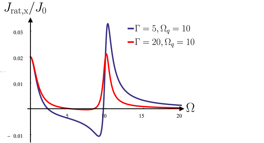
Figure 1: Dependence of the ratchet current on dimensionless frequency, $\Omega=\omega\tau,$ at two values of $\Gamma.$ For $\Gamma=20$ (red curve) there are two peaks: the Drude peak at $\Omega=0$ and the plasmonic resonance at $\Omega=\Omega_{q}$ in agreement with Ref. Rozhansky et al. (2015). With decreasing $\Gamma$ up to lower value $\Gamma=5$ (blue curve), the plasmonic resonance modifies and becomes strongly asymmetric [see Eq. (26)].

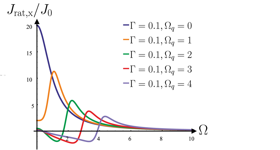
Figure 2: Dependence of the ratchet current on the dimensionless frequency for fixed small $\Gamma$ and different values of the quality factor of the plasmonic resonance, $\Omega_{q}.$ For $\Omega_{q}=0,$ plasmonic resonance is absent and response shows the Drude resonance at $\Omega=0.$ With increasing the quality factor, the asymmetric plasmonic peak appears.

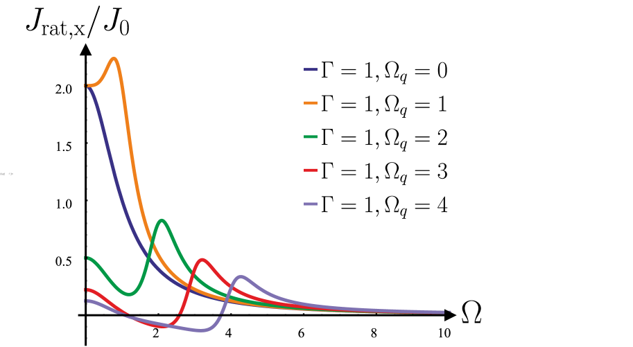
Figure 3: The same as in Fig. 2 but at lrger value of $\Gamma.$

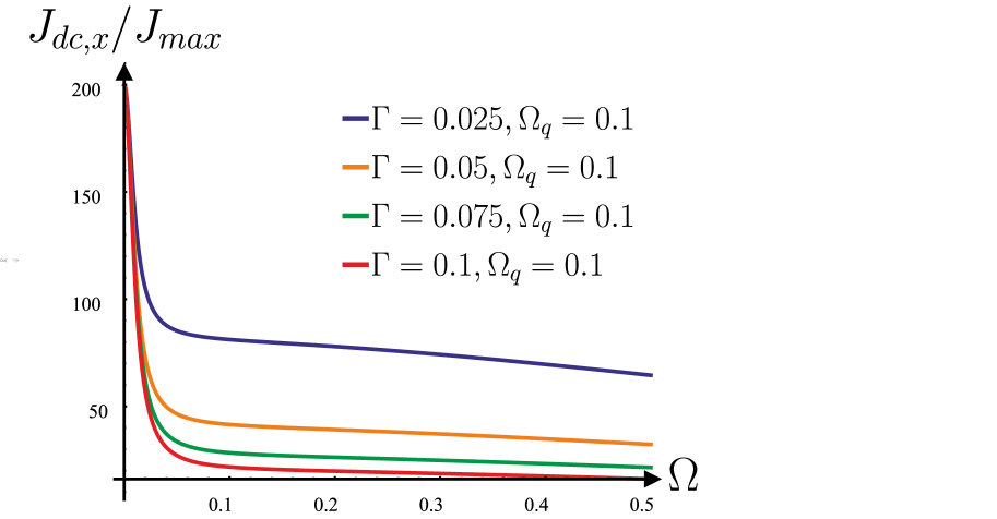
Figure 4: Non-resonant response for low quality factor $\Omega_{q}=0.1$ and small values of $\Gamma.$ Narrow peak at $\Omega=0$ arises on the top of the smooth Drude peak due to the Maxwell relaxation

Dependence of the ratchet current on the dimensionless frequency for various values of $\Gamma$ and $\Omega_{q}$ is shown in Figs. 1, 2, 3 for the case of linear polarization along the $x$ axis.

In Fig. 1 we plot the ratchet current as a function of the dimensionless frequency $\Omega$ for two values of $\Gamma.$ For large value $\Gamma=20$ the results of Ref. Rozhansky et al. (2015) are reproduced. Specifically, dc response shows the Drude peak at $\Omega=0$ and the plasmonic resonance at $\Omega=\Omega_{q}$ in agreement with Ref. Rozhansky et al. (2015). With decreasing $\Gamma$ the plasmonic resonance becomes asymmetric and changes sign in some interval of the frequencies. The evolution of the resonance from symmetric to asymmetric shape is well described by Eq. (26).

Figures 2 and 3 illustrate the plasmonic effect in the regime of small $\Gamma,$ when thermoelectric correction dominates. At zero plasmonic frequency, $\Omega_{q}=0,$ the dc response is given by the polarization-independent Seebeck peak having the Drude shape [see, Eq. (24)]. For sufficiently large quality factor, $\Omega_{q}\geq 1,$ there appear an asymmetric plasmonic resonance at $\Omega=\Omega_{q}.$

Most interesting behavior is obtained at small $\Gamma,$ when thermoelectric contribution is large, in the non-resonant regime, for $\Omega_{q}\ll 1.$ This case is illustrated in Fig. 4. As one can see a very narrow peak appears on the top of the smooth Drude dependence. Physics behind this peak is the Maxwell charge relaxation, which has a characteristic frequency scale $\Omega\sim\Omega_{q}^{2}\ll 1,$ i.e. for $\omega\sim\omega_{q}^{2}/\gamma\ll\gamma$ in dimensional units. For

$$\Omega_{q}\ll\sqrt{\Gamma}\ll 1,$$

analytical expression describing Fig. 4 can be found from Eq. (18) (where we put for simplicity $\tau_{\rm ee}=0$ ):

$$\frac{J_{\rm{rat},x}}{J_{0}}\approx\frac{\Omega_{q}^{2}}{\Omega^{2}+\Omega_{q}^{4}}+\frac{1}{\Gamma}\frac{1}{1+\Omega^{2}}.$$ (27)

Two terms here represent the Maxwell relaxation peak Rozhansky et al. (2015) and the Seebeck polarization-independent contribution

IV Viscous contribution

In this section we will discuss effect of finite viscosity of the electron liquid. We limit ourselves with the case of the linear polarization along $x$ direction and assume $\tau_{\rm ee}\ll\tau.$ Then, the electron liquid velocity is described by the Navier-Stokes equation:

$$\frac{\partial{v}}{\partial t}+\frac{{v}}{\tau}+s^{2}\frac{\partial n}{\partial x}-\eta\frac{\partial^{2}v}{\partial^{2}x}=a-v\frac{\partial v}{\partial x}\left(1+\frac{2}{\Gamma}\right),$$ (28)

We demonstrate below that effect of viscosity on the electronic ratchet effect is small and give only small correction to the $J_{{\rm dc},x}.$ However, the viscosity gives the key contribution to the excitation of the so-called travelling directional plasmons, which can be excited along with the ratchet dc current provided grating gate structure does not have inversion center Popov et al. (2015); Fateev et al. (2019); Moiseenko et al. (2020); Morozov and Fateev (2021).

IV.1 Small correction to the electronic ratchet current

Next, we discuss viscosity-induced correction to the electronic ratchet. We take into account that viscosity has dispersion described by the following equation Alekseev (2018):

$$\eta\to\eta(\omega)=\frac{\eta(0)}{1-i\omega\tau_{\rm ee}}.$$ (29)

The calculations are fully analogous to the ones presented in Appendix A.1. The details of calculations of the viscosity-induced correction as well as the most general formula for the dc ratchet current with account of the viscosity, Eq. (LABEL:J-eta), are presented in Appendix B. Analyzing Eq. (LABEL:J-eta) one can see that viscosity gives a small contribution to the ratchet current in the whole frequency interval. Here, we illustrate it for the case of high-frequency asymptotic. To this end we expand Eq. (LABEL:J-eta) up to linear order with respect to $\eta$ and assume that $\Omega\gg\Omega_{q}.$ The linear in $\eta$ term contains factor $Q^{2}\ll 1.$ We neglect $Q$ in this term everywhere except this factor. Then, we obtain

$$\frac{J_{\rm{rat},x}}{J_{0}} \approx\frac{\Omega_{q}^{2}}{\Omega^{6}}+\frac{1}{\Omega^{2}}\left(\frac{1}{\Gamma}+\frac{\tau_{\rm ee}}{2}\right)$$ (30)

$$+\frac{\eta Q^{2}}{1+\Omega^{2}\tau_{\rm ee}^{2}}\left(\frac{1-\tau_{\rm ee}\Omega^{2}}{\Gamma\Omega^{4}}-\frac{\tau_{\rm ee}}{2\Omega^{2}}\right),$$

where we use dimensionless units for $\tau_{\rm ee}$ (measured in the units of $\tau$) and $\eta$ (measured in the units of $v_{\rm F}^{2}\tau.$).

The first line of this equation represents asymptotic of Eq. (18) at $\Omega\to\infty.$ The second line represents viscosity-induced correction. The collision time $\tau_{\rm ee}$ appears in this correction due to dispersion of $\eta.$ It is worth noting that at $\Gamma\to\infty$ viscosity term in non-zero only due to this dispersion. Having in mind that dimensionless $\eta$ equals to $\tau_{ee}/4\tau,$ one can easily see that viscosity gives a small correction for any $\Gamma.$ At very high frequency this correction scales as $1/\Omega^{4}.$

IV.2 Viscosity-driven directional plasmons

In this subsection, we demonstrate that viscosity of the electron liquid, alhtough yielding a small correction to the electron ratchet effect, fully determines excitation of travelling directional plasmons Popov et al. (2015); Fateev et al. (2019); Moiseenko et al. (2020); Morozov and Fateev (2021).

Physics behind directional plasmons is as follows. Let us consider plasmonic oscillations of the density in the channel. Perturbation theory yields two terms which oscillate both in $t$ and in $x$: term of the first order $n^{(1,0)}$ and the second order term $n^{(1,1)}.$ The sum of these terms can be presented as two waves propagating in the opposite directions

$$n^{(1,0)}+n^{(1,1)}= C_{1}\cos(qx-\omega t-\alpha_{1})$$ (31)

$$+C_{2}\cos(qx+\omega t-\alpha_{2}),$$

where $C_{1,2}$ and $\alpha_{1,2}$ are the amplitudes and phases of these waves, respectively.

Since the grating gate structure does not have inversion center, the symmetry of the problem allows for $C_{1}\neq C_{2}.$ Then, the number of right- and left-moving plasmons is different and one can define

$$S_{\rm{pl}}=s(C_{1}^{2}-C_{2}^{2})$$ (32)

as a flux of directional plasmons travelling in a certain direction. Calculation of $S_{\rm pl}$ is presented in the Appendix C. In the limit $\eta\to 0,$ the result reads

$$\frac{S_{\rm{pl}}}{S_{0}}=\frac{\Omega}{(1+\Omega^{2})((\Omega^{2}-\Omega_{q}^{2})^{2}+\Omega^{2})},$$ (33)

where

$$S_{0}=\frac{e^{3}\tau^{5}q^{4}h|E_{0}|^{2}U_{0}\eta\sin\phi}{m^{3}s}\propto\eta~{}\Xi$$ (34)

We see that $S_{0}$ is proportional to $\eta$ (we neglect here terms of the order of $\eta^{2}$ and higher order). Hence, remarkably, the directed travelling plasmons are absent in the ideal electron liquid and appear only due to viscosity. We also see that $S_{0}$ as expected is proportional to the asymmetry parameter $\Xi.$ We also notice that $S_{\rm{pl}}$ does not depend on $\Gamma.$

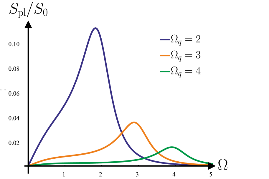
Figure 5: Dependence of the directed plasmons flux on the dimensionless frequency for different quality factors

Dependence of the directed plasmons flux on the dimensionless frequency is plotted in Fig. 5. This dependence contains symmetric plasmonic resonsnce similar to the resonance is dc ratchet current for $\Gamma\to\infty$. However, in contrast to electronic ratchet, the resonance at $\Omega=0$ is absent.

V Conclusion

To conclude, we have studied thermoelectric and viscous contributions to the radiation-induced electron ratchet current $J_{\rm rat}$ and to the flux of the travelling directional plasmons, $S_{\rm pl},$ in asymmetric dual-grating gate structure without inversion center. We have demonstrated that thermoelectric effects do not change $S_{\rm pl}$ but dramatically modify $J_{\rm rat}.$ By contrast, viscosity of the electron liquid leads to a small correction to $J_{\rm rat}$ but fully determines the flux of directed plasmons.

Appendix A Calculation of the ratchet current within a simplified method for $T\ll E_{\rm F}$

A.1 Linear polarization

In this Appendix, we present derivation of photo-induced dc current, $J_{\rm rat},$ within a simplified approach, which is valid in the strongly degenerated Fermi gas, when $T\ll E_{\rm F}.$ The approach is based on perturbative solution of simplified HD equations Eq. (13) and Eq. (14) with respect to external perturbation $a$. DC current appears in the order (2,1), i.e. is proportional to $hE_{0}^{2}U_{0},$ and can be presented as a sum two terms:

$$J_{{\rm rat},x}=\frac{e\tau}{m}N_{0}\left\langle na_{x}\right\rangle^{(2,1)}_{t,x}=J_{{\rm rat},x}^{\rm I}+J_{{\rm rat},x}^{\rm II},$$ (35)

where

$$J_{{\rm rat},x}^{\rm I}=-\frac{e\tau}{m}N_{0}\left\langle n^{(2,0)}\frac{\partial U}{\partial x}\right\rangle_{t,x},$$ (36)

$$J_{{\rm rat},x}^{\rm II}=\frac{e\tau}{m}N_{0}\left\langle n^{(1,1)}E_{x}\right\rangle_{t,x}$$ (37)

Hence, instead of calculation of the third order perturbative contribution to the current it is sufficient to calculate the second order correction to the dimensionless concentration $n.$

We start with calculation of the linear response: $n^{(1,0)},n^{(0,1)},v^{(1,0)},v^{(0,1)}$. Linearizing Eqs. (13) and  (14), we find:

$$n^{(1,0)}=-\frac{ehE_{0}q\sin(qx)}{2m(\omega_{q}^{2}-\omega^{2}-i\gamma\omega)}e^{-i\omega t}+h.c.,$$ (38)

$$v^{(1,0)}=-\frac{eE_{0}}{2m(\gamma-i\omega)}e^{-i\omega t}-\frac{ehE_{0}\omega\cos(qx)}{2im(\omega_{q}^{2}-\omega^{2}-i\gamma\omega)}e^{-i\omega t}+h.c.,$$

$$n^{(0,1)}=\frac{eV_{0}}{ms^{2}}\cos(qx+\theta),$$

$$v^{(0,1)}=0.$$

Substituting Eq. (38) into nonlinear terms one can perform high order iteration and do the next iterations by using the following matrix equation:

$$\begin{pmatrix}n\\ v\end{pmatrix}^{(i,j)}=\frac{1}{is^{2}\hat{q}^{2}+\hat{\omega}\gamma-i\hat{\omega}^{2}}\begin{pmatrix}i\gamma-\hat{\omega}&\hat{q}\\ \hat{q}s^{2}&\hat{\omega}\end{pmatrix}~{}\begin{pmatrix}J_{n}\\ J_{v}\end{pmatrix}^{(i,j)},$$ (39)

where $\hat{q}=-i\partial_{x}$, $\hat{\omega}=-i\partial_{t}$ and

$$\begin{pmatrix}J_{n}\\ J_{v}\end{pmatrix}^{(i,j)}=\begin{pmatrix}\partial_{x}(nv_{x})\\ v_{x}\partial_{x}v_{x}\left(1+2/\Gamma\right)\end{pmatrix}^{(i,j)},$$ (40)

are non-linear sources arising in the $(i,j)$ order of the perturbation expansion. In order to calculate $n^{(2,0)}$ and $n^{(1,1)},$ we need to calculate

$$\left(\begin{array}[]{c}J_{n}\\ J_{v}\end{array}\right)^{(2,0)}=\left(\begin{array}[]{c}-\partial_{x}(v^{(1,0)}n^{(1,0)})\\ -v^{(1,0)}\partial_{x}v^{(1,0)}(1+2/\Gamma)\end{array}\right),$$ (41)

and

$$\left(\begin{array}[]{c}J_{n}\\ J_{v}\end{array}\right)^{(1,1)}=\left(\begin{array}[]{c}-\partial_{x}(v^{(1,0)}n^{(0,1)})\\ 0\end{array}\right),$$ (42)

where $n^{(1,0)},n^{(0,1)},v^{(1,0)}$ are given by Eq. (38). After some algebra, we get

$$n^{(2,0)}=n^{(2,0)}(x)=\frac{e^{2}|E_{0}|^{2}h\cos{(qx)}(-\gamma\Gamma+i(2+\Gamma)\omega)}{4s^{2}m^{2}\Gamma(\gamma+i\omega)(\omega_{q}^{2}-\omega(i\gamma+\omega))}+h.c.,$$ (43)

$$n^{(1,1)}=n^{(1,1)}(x,t)=-\frac{e^{2}E_{0}U_{0}q\sin{(qx+\theta)}}{2s^{2}m^{2}(\omega_{q}^{2}-\omega(i\gamma+\omega))}e^{-i\omega t}+h.c..$$

Here, we left only time-independent terms in $n^{(2,0)},$ skipping terms $\exp(\pm 2i\omega t),$ which do not give contribution to the $dc$ response. Substituting Eq. (43) into Eqs. (36) and (37), we finally arrive at

$$\frac{J^{\rm I}_{{\rm rat},x}}{J_{0}}=\frac{\left((2+\Gamma)\omega^{2}(\omega^{2}-\omega_{q}^{2})+\gamma^{2}((2+\Gamma)\omega^{2}+\Gamma\omega_{q}^{2})\right)}{\tau^{2}\Gamma(\gamma^{2}+\omega^{2})(\gamma^{2}\omega^{2}+(\omega^{2}-\omega_{q}^{2})^{2})},$$ (44)

$$\frac{J^{\rm II}_{{\rm rat},x}}{J_{0}}=\frac{\left(\omega_{q}^{2}-\omega^{2}\right)}{\tau^{2}(\gamma^{2}\omega^{2}+(\omega^{2}-\omega_{q}^{2})^{2})},$$ (45)

A.2 Arbitrary polarization

Calculations presented in Appendix A.1 can be easily generalized for the case of arbitrary polarization, when the electric field is given by Eq. (20) and Eq. (21). In this case, hydrodynamic equations involve also $y-$component of the velocity:

$$\frac{\partial n}{\partial t}+\frac{\partial[(1+n)v_{x}]}{\partial x}=0,$$ (46)

$$\frac{\partial v_{x}}{\partial t}+\frac{v_{x}}{\tau}+s^{2}\frac{\partial n}{\partial x}=a_{x}-\left(1+\frac{2}{\Gamma}\right)v_{x}\frac{\partial v_{x}}{\partial x}-\frac{2}{\Gamma}v_{y}\frac{\partial v_{y}}{\partial x},$$ (47)

$$\frac{\partial v_{y}}{\partial t}+\frac{v_{y}}{\tau}=a_{y}-v_{x}\frac{\partial v_{y}}{\partial x},$$ (48)

where $a_{x}=e/m(E_{x}-\partial U/\partial x)$,$a_{y}=eE_{y}/m$. The calcaulations are fully analogous to the ones presented in Appendix A.1. Here, we present most important modifications without going into technical details. We start with calculation of the linear response: $n^{(1,0)},n^{(0,1)},v_{x}^{(1,0)},v_{y}^{(1,0)},v_{x}^{(0,1)}$. Linearizing Eqs. (46),  (47) and (48), we find:

$$n^{(1,0)}=-\frac{ehE_{0x}q\sin(qx)}{2m(\omega_{q}^{2}-\omega^{2}-i\gamma\omega)}e^{-i\omega t}+h.c.,$$ (49)

$$v_{x}^{(1,0)}=-\frac{eE_{0x}}{2m(\gamma-i\omega)}e^{-i\omega t}-\frac{ehE_{0x}\omega\cos(qx)}{2im(\omega_{q}^{2}-\omega^{2}-i\gamma\omega)}e^{-i\omega t}+h.c.,$$

$$v_{y}^{(1,0)}=-\frac{eE_{0y}(1+h\cos(qx))}{2m(-\gamma+i\omega)}e^{-i(\omega t+\theta)}+h.c.,$$

$$n^{(0,1)}=\frac{eV_{0}}{ms^{2}}\cos(qx+\theta),$$

$$v^{(0,1)}=0.$$

where $E_{0x}=E_{0}\cos\alpha,E_{0y}=E_{0}\sin\alpha$.Substituting Eq. (49) into nonlinear terms one can perform high order iteration and do the next iterations by using the following matrix equation:

$$\begin{pmatrix}n\\ v_{x}\\ v_{y}\end{pmatrix}^{(i,j)}=\frac{-i}{s^{2}\hat{q}^{2}-\hat{\omega}(i\gamma+\hat{\omega})}\begin{pmatrix}i\gamma+\hat{\omega}&\hat{q}&0\\ \hat{q}s^{2}&\hat{\omega}&0\\ 0&0&\hat{\omega}-\frac{\hat{q}^{2}s^{2}}{i\gamma+\hat{\omega}}\end{pmatrix}~{}\begin{pmatrix}J_{n}\\ J_{vx}\\ J_{vy}\end{pmatrix}^{(i,j)},$$ (50)

where $\hat{q}=-i\partial_{x}$, $\hat{\omega}=-i\partial_{t}$ and

$$\begin{pmatrix}J_{n}\\ J_{vx}\\ J_{vy}\end{pmatrix}^{(i,j)}=\begin{pmatrix}-\partial_{x}(nv_{x})\\ -v_{x}\partial_{x}v_{x}\left(1+2/\Gamma\right)-(2/\Gamma)v_{y}\partial_{x}v_{y}\\ -v_{x}\partial_{x}v_{y}\end{pmatrix}^{(i,j)},$$ (51)

are non-linear sources arising in the $(i,j)$ order of the perturbation expansion. In order to calculate $n^{(2,0)}$ and $n^{(1,1)},$ we need to calculate

$$\left(\begin{array}[]{c}J_{n}\\ J_{vx}\\ J_{vy}\end{array}\right)^{(2,0)}=\left(\begin{array}[]{c}-\partial_{x}(v_{x}^{(1,0)}n^{(1,0)})\\ -v^{(1,0)}\partial_{x}v^{(1,0)}(1+2/\Gamma)-(2/\Gamma)v_{y}^{(1,0)}\partial_{x}v_{y}^{(1,0)}\\ v_{x}^{(1,0)}\partial_{x}v_{y}^{(1,0)}\end{array}\right),$$ (52)

and

$$\left(\begin{array}[]{c}J_{n}\\ J_{vx}\\ J_{vy}\end{array}\right)^{(1,1)}=\left(\begin{array}[]{c}-\partial_{x}(v_{x}^{(1,0)}n^{(0,1)})\\ 0\\ 0\end{array}\right),$$ (53)

where $n^{(1,0)},n^{(0,1)},v^{(1,0)}$ are given by Eq. (49). After some algebra, we get

$$n^{(2,0)}=n^{(2,0)}(x)=\frac{e^{2}|E_{0}|^{2}h\cos{(qx)}}{4m^{2}s^{2}\Gamma}\left(\frac{(\gamma\Gamma-i\omega(2+\Gamma))\cos^{2}\alpha}{(\gamma+i\omega)(i\gamma\omega+\omega^{2}-\omega_{q}^{2})}-\frac{2\sin^{2}\alpha}{\gamma^{2}+\omega^{2}}\right)+h.c.,$$ (54)

$$n^{(1,1)}=n^{(1,1)}(x,t)=-\frac{e^{2}E_{0}U_{0}q\cos\alpha\sin{(qx+\theta)}}{2s^{2}m^{2}(\omega_{q}^{2}-\omega(i\gamma+\omega))}e^{-i\omega t}+h.c..$$

We will find the DC current $\mathbf{J}_{\rm{rat}}$ by the following formula

$$\mathbf{J}_{\rm{rat}}=\frac{e\tau}{m}N_{0}\left\langle n^{(1,1)}\mathbf{E}-n^{(2,0)}\frac{\partial U}{\partial x}\mathbf{e_{x}}\right\rangle_{t,x}$$ (55)

Substituting $n^{(1,1)}$ and $n^{(2,0)}$ into Eq. (55), we get $J_{\rm{rat,x}}$ and $J_{\rm{rat,y}}$:

$$\frac{J_{\rm{rat,x}}}{J_{0}}=\frac{P_{0}[2\omega^{4}-3\omega^{2}\omega_{q}^{2}+\omega_{q}^{4}+\gamma(2\omega^{2}+\Gamma\omega_{q}^{2})]+P_{\rm L1}~{}\omega_{q}^{2}(\gamma^{2}\Gamma+\omega^{2}-\omega_{q}^{2}))}{\tau^{2}\Gamma(\gamma^{2}+\omega^{2})(\gamma^{2}\omega^{2}+(\omega^{2}-\omega_{q}^{2})^{2}}$$ (56)

$$\frac{J_{{\rm rat},y}}{J_{0}}=\frac{(\omega_{q}^{2}-\omega^{2})P_{L2}+\gamma\omega P_{c}}{2\tau^{2}(\gamma^{2}\omega^{2}+(\omega^{2}-\omega_{q}^{2})^{2})}.$$ (57)

Appendix B Viscosity contribution

In this Appendix, we solve Eq. (28) together with Eq. (46) (with $v_{x}=v$). The calcaulations are fully analogous to the ones presented in Appendix A.1. Here, we present most important modifications without going into technical details. We start with calculation of the linear response: $n^{(1,0)},~{}n^{(0,1)},~{}v^{(1,0)},~{}v^{(0,1)}$. Linearizing Eqs. (46) and  (28) we find:

$$n^{(1,0)}=-\frac{ehE_{0}q\sin(qx)}{2m(\omega_{q}^{2}-\omega^{2}-i\gamma\omega)-iq^{2}\omega\eta(\omega))}e^{-i\omega t}+h.c.,$$ (58)

$$v^{(1,0)}=-\frac{eE_{0}}{2m(\gamma-i\omega)}e^{-i\omega t}-\frac{ehE_{0}\omega\cos(qx)}{2im(\omega_{q}^{2}-\omega(\omega+i\gamma)-iq^{2}\omega\eta(\omega))}e^{-i\omega t}+h.c.,$$

$$n^{(0,1)}=\frac{eV_{0}}{ms^{2}}\cos(qx+\theta),$$

$$v^{(0,1)}=0.$$

Substituting Eq. (49) into nonlinear terms one can perform high order iteration and do the next iterations by using the following matrix equation:

$$\begin{pmatrix}n\\ v\end{pmatrix}^{(i,j)}=\frac{-i}{s^{2}\hat{q}^{2}-\hat{\omega}(i\gamma+\hat{\omega})-i\hat{q}^{2}\hat{\omega}\hat{\eta}}\begin{pmatrix}i\gamma+\hat{\omega}+i\hat{q}^{2}\hat{\omega}\hat{\eta}&\hat{q}\\ \hat{q}s^{2}&\hat{\omega}\\ \end{pmatrix}~{}\begin{pmatrix}J_{n}\\ J_{v}\end{pmatrix}^{(i,j)},$$ (59)

where $\hat{q}=-i\partial_{x}$, $\hat{\omega}=-i\partial_{t}$, $\hat{\eta}=\eta/(1-i\hat{\omega}\tau_{ee})$ , $J_{n}$ and $J_{v}$ are determined by Eq. (40).Next, we repeat the steps described in appendix (A.1), and get $n^{(1,1)}$ and $n^{(2,0)}$:

$$n^{(2,0)}=n^{(2,0)}(x)=\frac{e^{2}|E_{0}|^{2}h\cos{(qx)}(-\gamma\Gamma+i(2+\Gamma)\omega-q^{2}\Gamma\eta(0))}{4m^{2}s^{2}\Gamma(\gamma+i\omega)(\omega_{q}^{2}-(i\gamma+\omega)\omega-iq^{2}\omega\eta(\omega))}+h.c.,$$ (60)

$$n^{(1,1)}=n^{(1,1)}(x,t)=-\frac{e^{2}E_{0}U_{0}q\sin{(qx+\theta)}(i\gamma+\omega+iq^{2}\eta(\omega))}{2s^{2}m^{2}(i\gamma+\omega)(\omega_{q}^{2}-\omega(i\gamma+\omega)-iq^{2}\omega\eta(\omega))}e^{-i\omega t}+h.c..$$

Substituting $n^{(1,1)}$ and $n^{(2,0)}$ into Eq. (15), we find total current for viscosity with arbitrary dispersion $\eta(\omega)$:

$$\frac{J_{{\rm rat},x}}{J_{0}}=\frac{(\gamma-i\omega)(2\gamma\Gamma-2i\omega+q^{2}\Gamma\eta(0))+q^{2}\Gamma(\gamma+i\omega)\eta(\omega)}{\tau^{2}\Gamma(\gamma^{2}+\omega^{2})(\omega_{q}^{2}-(i\gamma+\omega)\omega-iq^{2}\omega\eta(\omega))}+h.c.$$ (61)

We assume that viscosity $\eta(\omega)$ has the following dispersion Ref. Alekseev (2018):

$$\eta(\omega)=\frac{\eta}{1-i\omega\tau_{ee}},$$ (62)

where $\tau_{ee}$ is the electron-electron collision time. Then, the dc photoresponse is given by

$$\frac{J_{\rm{rat,x}}}{J_{0}}=\frac{1}{\tau^{2}\Gamma}\frac{2(1+\tau_{ee}^{2}\omega^{2})(\omega^{4}-\omega^{2}\omega_{q}^{2}+\gamma(\omega^{2}+\Gamma\omega_{q}^{2}))}{(\gamma^{2}+\omega^{2})((1+\tau_{ee}^{2}\omega^{2})(\gamma^{2}\omega^{2}+(\omega^{2}-\omega_{q}^{2})^{2}))+2q^{2}\eta\omega^{2}(\gamma+\tau_{ee}(\omega_{q}^{2}-\omega^{2}))}+$$ (63)

$$+\frac{1}{\tau^{2}\Gamma}\frac{q^{2}\eta\left[\omega^{2}\gamma(2+\gamma\Gamma\tau_{ee})+\omega^{4}\tau_{ee}(\Gamma-2)+\Gamma\omega_{q}^{2}(2\gamma+\tau_{ee}\omega^{2}(\gamma\tau_{ee}-1))\right]}{(\gamma^{2}+\omega^{2})((1+\tau_{ee}^{2}\omega^{2})(\gamma^{2}\omega^{2}+(\omega^{2}-\omega_{q}^{2})^{2}))+2q^{2}\eta\omega^{2}(\gamma+\tau_{ee}(\omega_{q}^{2}-\omega^{2}))}$$

Appendix C Directed plasmons

Oscillating contributions to the concentration $n^{(1,1)},$ and $n^{(1,0)}$ calculated in the previous section can be easily presented as:

$$n^{(1,0)}=A_{1}\cos(\omega t)\sin(qx)+B_{1}\sin(\omega t)\sin(qx),$$ (64)

$$n^{(1,1)}=A_{2}\cos(\omega t)\sin(qx+\phi)+B_{2}\sin(\omega t)\sin(qx+\phi),$$ (65)

where $A_{1},B_{1},A_{2},B_{2}$ are given by:

$$A_{1}=\frac{ehE_{0}q(\omega^{2}-\omega_{q}^{2})}{m(\gamma^{2}\omega^{2}+(\omega^{2}-\omega_{q}^{2})^{2}+q^{2}\eta\omega^{2}(2\gamma+q^{2}\eta))},$$ (66)

$$B_{1}=-\frac{ehE_{0}q\omega(\gamma+q^{2}\eta)}{m(\gamma^{2}\omega^{2}+(\omega^{2}-\omega_{q}^{2})^{2}+q^{2}\eta\omega^{2}(2\gamma+q^{2}\eta))},$$

$$A_{2}=\frac{e^{2}qE_{0}U_{0}\left[(\gamma^{2}+\omega^{2})(\omega^{2}-\omega_{q}^{2})+q^{2}\gamma\eta(2\omega^{2}-\omega_{q}^{2})+q^{4}\eta^{2}\omega^{2}\right]}{s^{2}m^{2}(\gamma^{2}+\omega^{2})((\omega^{2}-\omega_{q}^{2})^{2}+\gamma^{2}\omega^{2}+q^{2}\eta\omega^{2}(2\gamma+q^{2}\eta))},$$

$$B_{2}=-\frac{e^{2}qE_{0}U_{0}\omega\left[\gamma(\gamma^{2}+\omega^{2})+q^{2}\eta(\omega_{q}^{2}+2\gamma^{2})+q^{4}\eta^{2}\gamma\right]}{s^{2}m^{2}(\gamma^{2}+\omega^{2})((\omega^{2}-\omega_{q}^{2})^{2}+\gamma^{2}\omega^{2}+q^{2}\eta\omega^{2}(2\gamma+q^{2}\eta))}.$$

Here $\eta=\eta(0).$ The amplitudes $C_{1}$ and $C_{2}$ reads:

$$C_{1}=\frac{1}{2}\sqrt{(B_{1}+B_{2}\cos\phi+A_{2}\sin\phi)^{2}+(-B_{2}\sin\phi+A_{2}\cos\phi+A_{1})^{2}},$$ (67)

$$C_{2}=\frac{1}{2}\sqrt{(-B_{1}-B_{2}\cos\phi+A_{2}\sin\phi)^{2}+(B_{2}\sin\phi+A_{2}\cos\phi+A_{1})^{2}}$$ (68)

The flux of travelling directed plasmons is expressed through these coefficients as follows:

$$S_{\rm{pl}}=s(C_{1}^{2}-C_{2}^{2})=s(A_{2}B_{1}-A_{1}B_{2})\sin\phi$$ (69)

Substitutin Eq.  (66) into Eq. (69), and keeping linear in $\eta$ term only, we get

$$S_{\rm{pl}}=-\frac{e^{3}q^{4}|E_{0}|^{2}U_{0}\omega\eta\sin\phi}{sm^{3}(\gamma^{2}+\omega^{2})((\omega^{2}-\omega_{q}^{2})^{2}+\gamma^{2}\omega^{2})}.$$ (70)

Finally, by using dimensionless variables we arrive at Eq. (33) of the main text.

References

- Linke (2002) H. Linke, Appl. Phys. A 75, 167 (2002).
- Reimann (2002) P. Reimann, Phys. Rep. 361, 57 (2002).
- Hänggi and Marchesoni (2009) P. Hänggi and F. Marchesoni, Rev. Mod. Phys. 81, 387 (2009).
- Ivchenko and Ganichev (2011) E. L. Ivchenko and S. D. Ganichev, JETP Lett. 93, 673 (2011), [Pisma v ZhETF 93, 752 (2011)].
- Denisov et al. (2014) S. Denisov, S. Flach, and P. Hänggi, Phys. Rep. 538, 77 (2014).
- Cubero and Renzoni (2016) D. Cubero and F. Renzoni, in Brownian Ratchets (Cambridge University Press, 2016) pp. 13–26.
- Budkin et al. (2016) G. V. Budkin, L. E. Golub, E. L. Ivchenko, and S. D. Ganichev, JETP Lett. 104, 649 (2016).
- Reichhardt and Reichhardt (2017) C. J. O. Reichhardt and C. Reichhardt, Annu. Rev. Condens. Matter Phys. 8, 51 (2017).
- Ganichev et al. (2017) S. D. Ganichev, D. Weiss, and J. Eroms, Ann. Phys. 529, 1600406 (2017).
- Olbrich et al. (2011) P. Olbrich, J. Karch, E. L. Ivchenko, J. Kamann, B. März, M. Fehrenbacher, D. Weiss, and S. D. Ganichev, Phys. Rev. B 83, 165320 (2011).
- Otsuji et al. (2013) T. Otsuji, T. Watanabe, S. A. B. Tombet, A. Satou, W. M. Knap, V. V. Popov, M. Ryzhii, and V. Ryzhii, IEEE Trans. Terahertz Sci. Technol. 3, 63 (2013).
- Boubanga-Tombet et al. (2014) S. Boubanga-Tombet, Y. Tanimoto, A. Satou, T. Suemitsu, Y. Wang, H. Minamide, H. Ito, D. V. Fateev, V. V. Popov, and T. Otsuji, Appl. Phys. Lett. 104, 262104 (2014).
- Faltermeier et al. (2015) P. Faltermeier, P. Olbrich, W. Probst, L. Schell, T. Watanabe, S. A. Boubanga-Tombet, T. Otsuji, and S. D. Ganichev, J. Appl. Phys. 118, 084301 (2015).
- Olbrich et al. (2016) P. Olbrich, J. Kamann, M. König, J. Munzert, L. Tutsch, J. Eroms, D. Weiss, M.-H. Liu, L. E. Golub, E. L. Ivchenko, V. V. Popov, D. V. Fateev, K. V. Mashinsky, F. Fromm, T. Seyller, and S. D. Ganichev, Phys. Rev. B 93, 075422 (2016).
- Faltermeier et al. (2017) P. Faltermeier, G. V. Budkin, J. Unverzagt, S. Hubmann, A. Pfaller, V. V. Bel’kov, L. E. Golub, E. L. Ivchenko, Z. Adamus, G. Karczewski, T. Wojtowicz, V. V. Popov, D. V. Fateev, D. A. Kozlov, D. Weiss, and S. D. Ganichev, Phys. Rev. B 95, 155442 (2017).
- Olbrich et al. (2009) P. Olbrich, E. L. Ivchenko, R. Ravash, T. Feil, S. D. Danilov, J. Allerdings, D. Weiss, D. Schuh, W. Wegscheider, and S. D. Ganichev, Phys. Rev. Lett. 103, 090603 (2009).
- Popov et al. (2011) V. V. Popov, D. V. Fateev, T. Otsuji, Y. M. Meziani, D. Coquillat, and W. Knap, Appl. Phys. Lett. 99, 243504 (2011).
- Kannan et al. (2011) E. S. Kannan, I. Bisotto, J.-C. Portal, R. Murali, and T. J. Beck, Appl. Phys. Lett. 98, 193505 (2011).
- Nalitov et al. (2012) A. V. Nalitov, L. E. Golub, and E. L. Ivchenko, Phys. Rev. B 86, 115301 (2012).
- Kannan et al. (2012) E. S. Kannan, I. Bisotto, J.-C. Portal, T. J. Beck, and L. Jalabert, Appl. Phys. Lett. 101, 143504 (2012).
- Kurita et al. (2014) Y. Kurita, G. Ducournau, D. Coquillat, A. Satou, K. Kobayashi, S. B. Tombet, Y. M. Meziani, V. V. Popov, W. Knap, T. Suemitsu, and T. Otsuji, Appl. Phys. Lett. 104, 251114 (2014).
- Rozhansky et al. (2015) I. Rozhansky, V. Kachorovskii, and M. Shur, Phys. Rev. Lett. 114, 246601 (2015).
- Bellucci et al. (2016) S. Bellucci, L. Pierantoni, and D. Mencarelli, Integr. Ferroelectr. 176, 28 (2016).
- Fateev et al. (2017) D. V. Fateev, K. V. Mashinsky, and V. V. Popov, Appl. Phys. Lett. 110, 061106 (2017).
- Faltermeier et al. (2018) P. Faltermeier, G. V. Budkin, S. Hubmann, V. V. Bel’kov, L. E. Golub, E. L. Ivchenko, Z. Adamus, G. Karczewski, T. Wojtowicz, D. A. Kozlov, D. Weiss, and S. D. Ganichev, Physica E 101, 178 (2018).
- Rupper et al. (2018) G. Rupper, S. Rudin, and M. Shur, Phys. Rev. Appl. 9, 064007 (2018).
- Yu (2018) A. Yu, J. Phys. D: Appl. Phys. 51, 395103 (2018).
- Hubmann et al. (2020) S. Hubmann, V. V. Bel’kov, L. E. Golub, V. Y. Kachorovskii, M. Drienovsky, J. Eroms, D. Weiss, and S. D. Ganichev, Phys. Rev. Research 2, 033186 (2020).
- Delgado-Notario et al. (2020) J. A. Delgado-Notario, V. Clericò, E. Diez, J. E. Velázquez-Pérez, T. Taniguchi, K. Watanabe, T. Otsuji, and Y. M. Meziani, APL Photonics 5, 066102 (2020).
- Sai et al. (2021) P. Sai, S. O. Potashin, M. Szoła, D. Yavorskiy, G. Cywiński, P. Prystawko, J. Łusakowski, S. D. Ganichev, S. Rumyantsev, W. Knap, and V. Y. Kachorovskii, Phys. Rev. B 104, 045301 (2021).
- Yahniuk and et al. (2024) Yahniuk and et al., arXiv:2402.03956 (2024).
- Hild and et al. (2024) Hild and et al., arXiv:2402.17540 (2024).
- Mönch et al. (2022) E. Mönch, S. O. Potashin, K. Lindner, I. Yahniuk, L. E. Golub, V. Y. Kachorovskii, V. V. Bel’kov, R. Huber, K. Watanabe, T. Taniguchi, J. Eroms, D. Weiss, and S. D. Ganichev, Phys. Rev. B 105, 045404 (2022).
- Mönch et al. (2023) E. Mönch, S. O. Potashin, K. Lindner, I. Yahniuk, L. E. Golub, V. Y. Kachorovskii, V. V. Bel’kov, R. Huber, K. Watanabe, T. Taniguchi, J. Eroms, D. Weiss, and S. D. Ganichev, Phys. Rev. B 107, 115408 (2023).
- Narozhny et al. (2017) B. N. Narozhny, I. V. Gornyi, A. D. Mirlin, and J. Schmalian, Ann. Phys. 529, 1700043 (2017).
- Lucas and Fong (2018) A. Lucas and K. C. Fong, J. Phys. Condens. Matter 30, 053001 (2018).
- Narozhny (2019) B. N. Narozhny, Ann. Phys. 411, 167979 (2019).
- Polini and Geim (2020) M. Polini and A. K. Geim, Phys. Today 73, 28 (2020).
- Gurzhi (1963) R. N. Gurzhi, J Exp Theor Phys 17, 521 (1963).
- Gurzhi (1965) R. N. Gurzhi, Soviet Physics JETP 20, 953 (1965).
- Gurzhi (1968) R. N. Gurzhi, Sov. Phys.-Uspekhi 11, 255 (1968).
- de Jong and Molenkamp (1995) M. J. M. de Jong and L. W. Molenkamp, Phys. Rev. B 51, 13389 (1995).
- Bandurin et al. (2016) D. A. Bandurin, I. Torre, R. K. Kumar, M. B. Shalom, A. Tomadin, A. Principi, G. H. Auton, E. Khestanova, K. S. Novoselov, I. V. Grigorieva, L. A. Ponomarenko, A. K. Geim, and M. Polini, Science 351, 1055 (2016).
- Crossno et al. (2016) J. Crossno, J. K. Shi, K. Wang, X. Liu, A. Harzheim, A. Lucas, S. Sachdev, P. Kim, T. Taniguchi, K. Watanabe, T. A. Ohki, and K. C. Fong, Science 351, 1058 (2016).
- Moll et al. (2016) P. J. W. Moll, P. Kushwaha, N. Nandi, B. Schmidt, and A. P. Mackenzie, Science 351, 1061 (2016).
- Ghahari et al. (2016) F. Ghahari, H.-Y. Xie, T. Taniguchi, K. Watanabe, M. S. Foster, and P. Kim, Phys. Rev. Lett. 116, 136802 (2016).
- Kumar et al. (2017) R. K. Kumar, D. A. Bandurin, F. M. D. Pellegrino, Y. Cao, A. Principi, H. Guo, G. H. Auton, M. B. Shalom, L. A. Ponomarenko, G. Falkovich, K. Watanabe, T. Taniguchi, I. V. Grigorieva, L. S. Levitov, M. Polini, and A. K. Geim, Nat. Phys. 13, 1182 (2017).
- Bandurin et al. (2018) D. A. Bandurin, A. V. Shytov, L. S. Levitov, R. K. Kumar, A. I. Berdyugin, M. B. Shalom, I. V. Grigorieva, A. K. Geim, and G. Falkovich, Nat. Commun. 9 (2018), 10.1038/s41467-018-07004-4.
- Braem et al. (2018) B. A. Braem, F. M. D. Pellegrino, A. Principi, M. Röösli, C. Gold, S. Hennel, J. V. Koski, M. Berl, W. Dietsche, W. Wegscheider, M. Polini, T. Ihn, and K. Ensslin, Phys. Rev. B 98, 241304 (2018).
- Jaoui et al. (2018) A. Jaoui, B. Fauqué, C. W. Rischau, A. Subedi, C. Fu, J. Gooth, N. Kumar, V. Süß, D. L. Maslov, C. Felser, and K. Behnia, npj Quantum Mater. 3 (2018), 10.1038/s41535-018-0136-x.
- Gooth and Kumar (2018) F. Gooth, J.and Menges and N. e. a. Kumar, Nat. Commun. 9 (2018), 10.1038/s41467-018-06688-y.
- Berdyugin et al. (2019) A. I. Berdyugin, S. G. Xu, F. M. D. Pellegrino, R. K. Kumar, A. Principi, I. Torre, M. B. Shalom, T. Taniguchi, K. Watanabe, I. V. Grigorieva, M. Polini, A. K. Geim, and D. A. Bandurin, Science , eaau0685 (2019).
- Gallagher et al. (2019) P. Gallagher, C.-S. Yang, T. Lyu, F. Tian, R. Kou, H. Zhang, K. Watanabe, T. Taniguchi, and F. Wang, Science , eaat8687 (2019).
- Sulpizio et al. (2019) J. A. Sulpizio, L. Ella, A. Rozen, J. Birkbeck, D. J. Perello, D. Dutta, M. Ben-Shalom, T. Taniguchi, K. Watanabe, T. Holder, R. Queiroz, A. Principi, A. Stern, T. Scaffidi, A. K. Geim, and S. Ilani, Nature 576, 75 (2019).
- Ella et al. (2019) L. Ella, A. Rozen, J. Birkbeck, M. Ben-Shalom, D. Perello, J. Zultak, T. Taniguchi, K. Watanabe, A. K. Geim, S. Ilani, and J. A. Sulpizio, Nat. Nanotechnol. 14, 480 (2019).
- Ku et al. (2020) M. J. H. Ku, T. X. Zhou, Q. Li, Y. J. Shin, J. K. Shi, C. Burch, L. E. Anderson, A. T. Pierce, Y. Xie, A. Hamo, U. Vool, H. Zhang, F. Casola, T. Taniguchi, K. Watanabe, M. M. Fogler, P. Kim, A. Yacoby, and R. L. Walsworth, Nature 583, 537 (2020).
- Raichev et al. (2020) O. E. Raichev, G. M. Gusev, A. D. Levin, and A. K. Bakarov, Phys. Rev. B 101, 235314 (2020).
- Gusev et al. (2020) G. M. Gusev, A. S. Jaroshevich, A. D. Levin, Z. D. Kvon, and A. K. Bakarov, Sci. Rep. 10 (2020), 10.1038/s41598-020-64807-6.
- Geurs et al. (2020) J. Geurs, Y. Kim, K. Watanabe, T. Taniguchi, P. Moon, and J. H. Smet, arXiv:2008.04862 [cond-mat.mes-hall] (2020).
- Kim et al. (2020) M. Kim, S. G. Xu, A. I. Berdyugin, A. Principi, S. Slizovskiy, N. Xin, P. Kumaravadivel, W. Kuang, M. Hamer, R. K. Kumar, R. V. Gorbachev, K. Watanabe, T. Taniguchi, I. V. Grigorieva, V. I. Fal’ko, M. Polini, and A. K. Geim, Nat. Commun. 11 (2020), 10.1038/s41467-020-15829-1.
- Vool et al. (2020) U. Vool, A. Hamo, G. Varnavides, Y. Wang, T. X. Zhou, N. Kumar, Y. Dovzhenko, Z. Qiu, C. A. C. Garcia, A. T. Pierce, J. Gooth, P. Anikeeva, C. Felser, P. Narang, and A. Yacoby, arXiv:2009.04477 [cond-mat.mes-hall] (2020).
- Gupta et al. (2021) A. Gupta, J. Heremans, G. Kataria, M. Chandra, S. Fallahi, G. Gardner, and M. Manfra, Phys. Rev. Lett. 126, 076803 (2021).
- Gusev et al. (2021) G. M. Gusev, A. S. Jaroshevich, A. D. Levin, Z. D. Kvon, and A. K. Bakarov, Phys. Rev. B 103, 075303 (2021).
- Zhang and Shur (2021) Y. Zhang and M. S. Shur, J. Appl. Phys. 129, 053102 (2021).
- Jaoui et al. (2021) A. Jaoui, B. Fauqué, and K. Behnia, Nat. Commun. 12 (2021), 10.1038/s41467-020-20420-9.
- Popov et al. (2015) V. V. Popov, D. V. Fateev, E. L. Ivchenko, and S. D. Ganichev, Phys. Rev. B 91, 235436 (2015).
- Fateev et al. (2019) D. V. Fateev, K. V. Mashinsky, J. D. Sun, and V. V. Popov, Solid-State Electron. 157, 20 (2019).
- Moiseenko et al. (2020) I. M. Moiseenko, V. V. Popov, and D. V. Fateev, Journal of Physics Communications 4, 071001 (2020).
- Morozov and Fateev (2021) V. Morozov, M.Y.and Popov and D. Fateev, Sci. Rep. , 11431 (2021).
- Alekseev (2018) P. S. Alekseev, Phys. Rev. B. 98, 165440 (2018).