Theory of possible sliding regimes in twisted bilayer WTe₂

Abstract

Inspired by the observation of increasingly one-dimensional (1D) behavior with decreasing temperature in small-angle twisted bilayers of WTe₂ (tWTe₂), we theoretically explore the exotic sliding regimes that could be realized in tWTe₂. At zero displacement field, while hole-doped tWTe₂ can be thought of as an array of weakly coupled conventional two-flavor 1D electron gases (1DEGs), the electron-doped regime is equivalent to coupled four-flavor 1DEGs, due to the presence of an additional “valley” degree of freedom. In the decoupled limit, the electron-doped system can thus realize phases with a range of interesting ordering tendencies, including $4k_{F}$ charge-density-wave and charge-$4e$ superconductivity. Dimensional crossovers and cross-wire transport due to inter-wire couplings of various kinds are also discussed. We find that a sliding Luther–Emery liquid with small inter-wire couplings is probably most consistent with current experiments on hole-doped tWTe₂.

Introduction.—One dimensional quantum electronic systems are the best understood examples of non-Fermi liquids, i.e. metals without coherent electronic quasiparticles. Indeed, the low energy elementary excitations in a 1D electron gas (1DEG) are all bosonic, and exhibit phenomena such as interaction-dependent power-law scaling of correlation functions and spin-charge separation [1, 2, 3, 4]. Besides the 1DEG, there also exist systems with quasi-1D properties in higher dimension, such as organic (super)conductors [5, 6, 7] and Cs₃As₃-chain based superconductors [8, 9, 10, 11]. Moreover, while the stripe phases of underdoped cuprates are not, in any literal sense, quasi-1D, it has been suggested that their unusual non-Fermi liquid and non-BCS properties can be obtained by considering adiabatic continuity from an artificial strongly stripe-ordered quasi-1D limit [12, 13, 14, 15, 16].

At low enough temperatures, $T<T_{\text{2D}}$, almost all quasi-1D systems ultimately crossover to states with some version of 2D coherence. However, there can exist “sliding phases” (e.g. sliding Luttinger or Luther–Emery liquids) [17, 18, 19, 20, 21, 22, 23, 24, 25, 26, 22, 27, 28, 29, 30, 31, 32] in which there is a parametrically broad temperature window, $T_{\text{2D}}<T<T_{\text{1D}}$, within which the intra-chain quantum dynamics is highly coherent but all inter-chain effects are incoherent and perturbative. Such a sliding metallic phase may have been observed in, e.g. lithium purple bronze (LiPB) [33, 34, 35, 36].

One essential question is how far can the sliding metal phase persist down in temperature, and might there exist circumstances in which it truly persists to $T\to 0$? Recent experiments on small angle twisted bilayer WTe₂ [tWTe₂, see Fig. 1(a)] have seemingly evinced an affirmative answer to this question [37, 38]. In common with other twisted bilayer transition-metal-dichalcogenides (TMDs) [39, 40, 41, 42, 43, 44, 45, 46, 47, 48, 49, 50, 51, 52, 53, 54, 55, 56, 57, 58, 59, 60, 61, 62, 63, 64, 65, 66], the properties of tWTe₂ are highly tunable (by varying twist angle and gate-controlled doping). This, combined with its anisotropic electronic structure, make it an ideal system to address these issues. Moreover, the nature of the sliding phases resulting from the emergence of multiple moiré bands remains largely unexplored.

In this paper, we study tWTe₂ from a theoretical perspective. As shown in Fig. 1(a), the stripe-like moiré pattern of tWTe₂ naturally lends itself to a model of weakly coupled 1D wires. We first explicitly construct the moiré band structures and show that both hole- and electron-doped tWTe₂ host quasi-1D moiré bands, with the hole-regime having weaker inter-wire hopping $t_{\bot}$. In the decoupled wire limit, while the hole-regime is a relatively conventional two-flavor 1DEG, the electron-regime realizes a four-flavor 1DEG. The existence of both spin and pseudospin flavors in the electron-regime results in a rich variety of possible favored correlations, even in the decoupled wire limit, including phases with dominant Wigner-crystal-like $4k_{F}$ charge-density-wave (CDW) [67, 68, 69, 70, 71] or charge-$4e$ superconducting [72, 73, 74, 75, 76, 77, 78, 79, 80, 81, 82] correlations. Moreover, from an analysis of the hole-doped regime, we conclude that the experimentally established bound on $T_{\text{2D}}$ reported in Ref. [38], as well as the most salient features of the anisotropic transport at the lowest accessible temperatures, can most readily be understood as reflecting the behavior of a sliding Luther–Emery (LE) liquid.

Model.—Monolayer 1T^′-WTe₂ has a rectangular unit cell, and its low energy electrons are from two $d$-orbitals on W atoms and two $p$-orbitals on Te atoms [83, 84], as shown in Fig. 1(a). The symmetries of the free-standing monolayer include lattice translations, time-reversal $\mathcal{T}$, three-dimensional inversion $\mathcal{P}$, and a glide mirror $\bar{M}_{y}$ that sends $(x,y,z)\mapsto(x,-y+a_{y}/2,z)$, where $a_{y}$ is the lattice constant in the $y$-direction. The combination of $\mathcal{P}$ and $\mathcal{T}$ ensures a two-fold (Kramers) degeneracy of each band. An $s_{z}$-conserving spin-orbit-coupling (SOC) opens a band gap at charge neutrality, and turns monolayer WTe₂ into a $\mathbb{Z}_{2}$ topological insulator [85, 86, 87]. With electron doping it becomes superconducting [88, 89, 90, 91, 92]. In Fig. 1(b) we show the band structure and Fermi pockets at small doping of monolayer WTe₂ based on the tight-binding model of Ref. [84]. Note that for hole doping there is a single Fermi pocket at the $\Gamma$ point, while for electron doping there are two well-separated pockets related by $\bar{M}_{y}\mathcal{P}\mathcal{T}$, which we label ‘u’ and ‘d’ respectively.

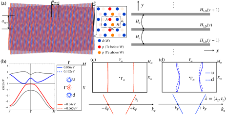
Figure 1: Emergent 1D physics in tWTe₂. (a) Moiré pattern shows 1D stripes, which we model as an array of weakly coupled wires. (b) Left panel - near zero energy band structure of monolayer WTe₂; red and blue are the valence and conduction bands. Right panel - electron and hole pockets at the indicated Fermi energies for doped WTe₂ obtained from Ref.[84]. Typical Fermi surfaces and reduced 1D model for the first moiré band(s) in hole- and electron-doped tWTe₂ ($\theta\approx 3^{\circ}$) are shown in (c) and (d) respectively.

In twisted bilayer WTe₂, both $\mathcal{P}$ and $\bar{M}_{y}$ are broken, but at small twist angle $\theta$ they remain approximate symmetries; in this regime the distinction between $\bar{M}_{y}$ and regular mirror $M_{y}$ is also unimportant at low energies. A displacement field breaks $\mathcal{P}$ but preserves $M_{y}$. In Figs. 1(c) and 1(d) we plot representative moiré Fermi surfaces for hole- and electron-doped tWTe₂ at $\theta\approx 3^{\circ}$ and zero displacement field, obtained using the continuum model approach [93, 94] [see the Supplementary Material (SM) [95] for details]. The hole regime can be described as a weakly-coupled array of conventional spinful 1DEGs, whose properties are characterized by charge and spin Luttinger parameters $K_{\mathrm{c}}$ and $K_{\mathrm{s}}$. The sliding regimes and dimensional crossovers in hole-doped tWTe₂ are therefore readily understood based on existing theoretical results [96, 97, 98, 99, 100, 101, 102, 103, 104]. The electron regime hosts fermions with an additional “valley” pseudospin $\tau_{z}=\mathrm{u},\mathrm{d}$ (which is conserved at small $\theta$ since the u- and d-pockets are decoupled in this limit), and hence realizes an array of four-flavor $\lambda=(s_{z},\tau_{z})$ 1DEGs. The symmetries ensure that (at zero displacement field) $k_{F}$ is identical for all flavors in the decoupled-wire limit [see Fig.1(d)].

The electron-doped regime of tWTe₂ can in principle realize a rich variety of phases due to its four flavors, and is the main focus of this paper. To proceed with the analysis, we bosonize each wire via four density operators

$$\hat{\rho}_{0}(x)=\tfrac{1}{2}\big{[}\hat{\rho}_{\uparrow,\mathrm{u}}(x)+\hat{\rho}_{\uparrow,\mathrm{d}}(x)+\hat{\rho}_{\downarrow,\mathrm{u}}(x)+\hat{\rho}_{\downarrow,\mathrm{d}}(x)\big{]},$$ (1)

$$\hat{\rho}_{1}(x)=\tfrac{1}{2}\big{[}\hat{\rho}_{\uparrow,\mathrm{u}}(x)+\hat{\rho}_{\uparrow,\mathrm{d}}(x)-\hat{\rho}_{\downarrow,\mathrm{u}}(x)-\hat{\rho}_{\downarrow,\mathrm{d}}(x)\big{]},$$

$$\hat{\rho}_{2}(x)=\tfrac{1}{2}\big{[}\hat{\rho}_{\uparrow,\mathrm{u}}(x)-\hat{\rho}_{\uparrow,\mathrm{d}}(x)+\hat{\rho}_{\downarrow,\mathrm{u}}(x)-\hat{\rho}_{\downarrow,\mathrm{d}}(x)\big{]},$$

$$\hat{\rho}_{3}(x)=\tfrac{1}{2}\big{[}\hat{\rho}_{\uparrow,\mathrm{u}}(x)-\hat{\rho}_{\uparrow,\mathrm{d}}(x)-\hat{\rho}_{\downarrow,\mathrm{u}}(x)+\hat{\rho}_{\downarrow,\mathrm{d}}(x)\big{]}.$$

Here the subscripts $0$–$3$ label, respectively, the total charge, spin, valley, and spin-valley densities. Their fluctuations are represented by bosonic fields $\phi_{i}(x)$ via $\delta\hat{\rho}_{i}(x)=-\partial_{x}\phi_{i}(x)/\pi$, with dual fields $\theta_{i}(x)$ defined such that $\Pi_{i}(x)=\partial_{x}\theta_{i}(x)/\pi$ is the conjugate momentum.

We consider the generic case in which the band filling is incommensurate, so umklapp scattering can be neglected, i.e. the Hamiltonian is invariant under $\phi_{0}(x)\to\phi_{0}(x)+\mathrm{const}$. The most general form of the effective Hamiltonian of a decoupled wire, respecting the symmetries of the problem ($\mathcal{T}$, $\mathcal{P}$ and $M_{y}$, as well as conservation of total $s_{z}$ and $\tau_{z}$) is then [95]

$$H_{1D} =\sum_{i=0}^{3}\frac{v_{i}}{2}\int dx\left\{\pi K_{i}[\Pi_{i}(x)]^{2}+\frac{1}{\pi K_{i}}[\partial_{x}\phi_{i}(x)]^{2}\right\}$$

$$-{\sum_{\{ijk\}}\frac{g_{i}}{(\pi\alpha)^{2}}}\int dx\,\cos[2\phi_{j}(x)]\cos[2\phi_{k}(x)],$$ (2)

where $v_{i}$ are the velocities of the four bosonic fields, $K_{i}$ are Luttinger parameters incorporating all forward-scattering interactions, $g_{i}$ are the strengths of the leading back-scattering interactions, $\alpha$ is a short-distance cutoff, and $\{i,j,k\}$ runs over the three cyclic permutations of $\{1,2,3\}$ . Note that the values of $v_{i}$, $K_{i}$ and $g_{i}$ are not constrained by the symmetries; in particular, the absence of $SU(2)$ symmetry for both spin and valley implies there is no reason to expect the $K_{i}$’s to be near $1$.

Of possible inter-wire couplings, a subset are forward-scattering interactions that couple the densities $\hat{\rho}_{i}$, or the conjugate currents, on neighboring wires. In bosonized form, these interactions are marginal, and can be treated exactly; they lead to a renormalization and proliferation of effective Luttinger parameters, but preserve the “sliding” symmetry of the system under arbitrary shifts of $\phi_{0}$ on each wire [18, 19, 20]. If large, these terms can have a qualitative effect on the dimensional crossover. However, these interactions are likely small in current experimental setups due to the screening by top and bottom gates, and hence can be neglected.

Thus, the crossover to higher-dimensional behavior is induced by inter-wire coupling of the form

$$H_{c}=-\sum_{a}J_{a}\sum_{y}\int dx\ O_{a}^{\dagger}(x,y)\,O_{a}(x,y+1)+\text{h.c.},$$ (3)

where $y\in\mathbb{Z}$ labels different wires and $a$ labels different couplings. If the decoupled wire remains gapless, single-particle hopping ($J_{e}=t_{\bot}$) is usually the dominant process, where $O_{e}^{\dagger}(x,y)\equiv\psi^{\dagger}(x,y)$ is just the fermion creation operator. However, when there are interaction-induced gaps on each wire, single-particle hopping is irrelevant at energies smaller than the gap, and higher-order processes are the key actors. Inter-wire interactions between particle-particle (e.g. charge-2e SC) or particle-hole (e.g. $2k_{F}$ CDW) orders are generated to second order in $t_{\bot}$, giving rise to a “bare” value of $J_{2e}\sim J_{2k_{F}}\sim t_{\bot}^{2}/w$  . We will also be interested in still higher order terms, especially charge-$4e$ SC and $4k_{F}$ CDW, both of which have bare values $J_{4e}\sim J_{4k_{F}}\sim t_{\bot}^{4}/w^{3}$.

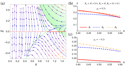
Figure 2: (a) RG flows from Eq. (4) in the invariant symmetric subspace $\tilde{g}_{j}=\tilde{g}$ and $K_{j}=K$. A fully gapless, stable Luttinger liquid fixed line is shown in solid red. The dashed red is an unstable LL fixed line. Beyond the separatrix (dotted blue) the system flows to strong coupling, indicating a maximally gapped generalized LE phase. Small perturbations that break the flavor symmetries scale away (flows converge on the represented plane) within the green region. (b) Solution of $\delta_{i}$’s in the unfrustrated fully gapped case obtained from Eq. (5). (c) Hierarchy in $\delta_{i}$’s in the frustrated fully gapped case. Here for simplicity we take $g_{1}=0.3v,g_{2}=0.25v$ and $v_{j}=v$.

Renormalization group (RG) analysis.—We first analyze the decoupled 1D wires. From Eq. (2) we see that the charge field $\phi_{0}(x)$ is absent from the cosine terms, and thus remains gapless, as required by the generalized Luttinger theorem [72]. If any of the cosine terms is relevant, this typically leads to the opening of a gap in the $\phi_{1}$, $\phi_{2}$, and/or $\phi_{3}$ sector without symmetry breaking, in which case the system can be viewed as a multi-component generalization of the LE liquid. To quadratic order in the dimensionless couplings $\tilde{g}_{i}\equiv g_{i}/\bar{v}$, where $\bar{v}\equiv(v_{1}+v_{2}+v_{3})/3$, the RG equations at $T\to 0$ are [95]

$$dK_{1}/dl =-K_{1}^{2}\big{[}\tilde{g}^{2}_{2}(A_{3}K_{3}+A_{1}K_{1})+\tilde{g}^{2}_{3}(A_{2}K_{2}+A_{1}K_{1})\big{]},$$

$$d\tilde{g}_{1}/dl =[2-(K_{2}+K_{3})]\tilde{g}_{1}+A_{1}^{\prime}\tilde{g}_{2}\tilde{g}_{3}K_{1},$$ (4)

and four other equations obtained by cyclic permutations of the indices $\{1,2,3\}$, where $A_{j}$ and $A_{j}^{\prime}$ are positive constants that depend on the relative velocities $v_{j}/\bar{v}$ and on the cutoff scheme . These non-linear equations define extremely complicated flows in a 6-dimensional coupling space, which we have extensively explored in various regimes. We find three qualitatively distinct sorts of “long RG-time” ($l\gg 1$) behavior (generalized basins of attraction) of these flows for distinct ranges of initial values of the (bare) interactions, as discussed below.

1) If $K_{i}+K_{j}>2$ for all $\{i,j\}$, all the $\tilde{g}_{k}$ are irrelevant, meaning that the ground state is a fully gapless Luttinger liquid (LL) with four gapless modes, each of which will generically have a different velocity. The power law correlations in this phase are governed by four continuously tunable (marginal) couplings, $K_{j}$ (including $K_{0}$).

2) If two factors $K_{i}+K_{j}>2$ and one is $<2$, the RG flows go to strong coupling along a trajectory in which one $\tilde{g}_{j}$ grows while the other two tend to zero, leading to a partially gapped generalized LE phase with two of the $\phi_{j}$’s gapped. For example, consider the case in which $K_{1}+K_{2}$ and $K_{1}+K_{3}>2$ but $K_{2}+K_{3}<2$. In this case, both $\tilde{g}_{2}$ and $\tilde{g}_{3}$ are irrelevant and only weakly renormalize $K_{1}$, so we need only consider the flows in the subspace $\tilde{g}_{2,3}=0$ and $K_{1}=\text{constant}$. In this subspace, $\epsilon\equiv 1/K_{3}-1/K_{2}$ is also an invariant. For $\epsilon=0$, the flows are exactly the same as those for the conventional two-flavor 1DEG, while for $\epsilon\neq 0$ they are qualitatively similar.

3) We have not found any condition in which only two of the $\tilde{g}_{j}$’s flow to strong coupling. Thus, the third case arises when all three flow to larger values, implying a maximally gapped generalized LE phase, in which only $\phi_{0}$ remains gapless, and $K_{0}$ determines the power-law decay of various correlation functions. The nature of the flow to strong coupling depends qualitatively on $\eta\equiv\operatorname{sgn}(\tilde{g}_{1}\tilde{g}_{2}\tilde{g}_{3})$. If $\eta=1$, there exist stable (attractive) trajectories along which all $|\tilde{g}_{j}|$ are equal, whereas similar trajectories are unstable if $\eta=-1$. Indeed for $\eta=-1$ the cosine terms in Eq. (2) resemble antiferromagnetically coupled Ising spins on a triangular lattice, and are thus frustrated, leading to the growth of an initial hierarchy among the $|\tilde{g}_{j}|$’s under the RG. In Fig. 2(a) we show the flows within the invariant symmetric subspace $\tilde{g}_{j}=\tilde{g}$ and $K_{j}=K$, highlighting the stable region in green.

Self-consistent gap equations.—Complementary to the weak coupling RG analysis, here we estimate the values of the gaps, $\Delta_{j}$, in the various strong-coupling limits. We solve the problem variationally, using a trial Gaussian action with mass terms as variational parameters [95]. In the case without frustration ($\eta=1$), the result is a set of coupled self-consistency conditions for the gaps:

$$\delta_{1}^{2}=\frac{4K_{1}}{\pi v_{1}}\,\delta_{1}^{K_{1}}\!\left(|g_{2}|\delta_{3}^{K_{3}}+|g_{3}|\delta_{2}^{K_{2}}\right),$$ (5)

and two similar equations obtained by cyclic permutations of the indices $\{1,2,3\}$, where $\delta_{i}\equiv\Delta_{i}/(v_{i}/\alpha)\ll 1$ is the dimensionless gap. The (always possible) solution to Eq. (5) with $\delta_{1}=0$ is physically relevant if $K_{1}+K_{2}$ and $K_{1}+K_{3}>2$ (i.e. if $g_{2}$ and $g_{3}$ are both irrelevant) while the non-zero solution is physical otherwise. Applying this same logic to all three gap equations we find, consistent with the RG results, that two of the three modes are gapped if only one $g_{j}$ is relevant; for instance, if only $g_{1}$ is relevant, then $\delta_{1}=0$ and $\delta_{2}\sim\delta_{3}\sim|g_{1}|^{1/(2-K_{2}-K_{3})}$ with $\delta_{2}/\delta_{3}=\sqrt{K_{2}v_{3}/K_{3}v_{2}}$. All three modes are gapped if either two or three of the $g_{j}$’s is relevant, and the induced gaps $\delta_{1,2,3}$ are generally comparable in magnitude, as shown in Fig. 2(b). In the case with frustration ($\eta=-1$), the gap equations are the same except that the smallest $|g_{j}|$ is replaced by $-|g_{j}|$  . Frustration suppresses the gaps unequally, resulting in a hierarchy in which two gaps are parametrically larger than the third [see Fig. 2(c) and the SM for more details].

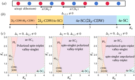
Figure 3: Phases of decoupled wires. (a) Schematic of the spatial order identified as WC, where red and blue represent u and d. (b) Phase diagram of the fully gapped system with phases identified with the most divergent susceptibility as $T\to 0$, with subleading divergences noted in parentheses. (c) Phase diagrams for partially gapped cases when the relevant $g_{i}>0$. Here CDW, SDW, VDW and SVDW are abbreviations for charge, spin, valley and spin-valley $2k_{F}$ density waves respectively.

Order parameters.—We now identify the order parameters with the slowest-decaying correlations, which determine the character of the 2D long-range order at $T\to 0$ when inter-wire couplings are included. A complete analysis of all such order parameters, up to fourth-order in fermion operators, is presented in the SM [95]. In different regimes, we find the leading orders to be various kinds of momentum-$2k_{F}$ and -$4k_{F}$ density waves ($O_{2k_{F}}\sim\psi_{R}^{\dagger}\psi_{L}$, $O_{4k_{F}}\sim\psi_{R}^{\dagger}\psi_{R}^{\dagger}\psi_{L}\psi_{L}$, where $\psi_{R,L}$ are right or left moving fermions with flavor indices omitted), charge-$2e$ and -$4e$ superconductivities ($O_{2e}\sim\psi_{R}\psi_{L}$, $O_{4e}\sim O_{2e}O_{2e}^{\prime}$), and zero momentum (Pomeranchuk) instabilities ($O_{\text{PI}}\sim O_{2e}^{\dagger}O_{2e}^{\prime}$). Some representative order parameters of each type in bosonized form are

$$O_{2k_{F}\text{-CDW}}\propto\left(\textstyle\prod_{j=1}^{3}\cos\phi_{j}-i\prod_{j=1}^{3}\sin\phi_{j}\right)e^{i\phi_{0}-i2k_{F}x},$$

$$O_{2e,j}\propto\cos(\phi_{k}\pm\phi_{i})e^{i(\theta_{0}\pm\theta_{j})},$$

$$O_{{4k_{F}}_{j}}\propto\cos(2\phi_{j})e^{i2\phi_{0}-i4k_{F}x},$$

$$O_{4e,j}\propto\cos(\phi_{k}+\phi_{i})\cos(\phi_{k}-\phi_{i})e^{i2\theta_{0}}$$

$$O_{\text{PI},j}\propto\cos(\phi_{k}+\phi_{i})\cos(\phi_{k}-\phi_{i})e^{i2\theta_{j}}.$$ (6)

Another interesting $4k_{F}$-order, which we identify as a “Wigner crystal” order $O_{\text{WC}}\propto\sin(2\phi_{1})e^{i2\phi_{0}-i4k_{F}x}$, is invariant under the combination of $x\to x+\pi/(4k_{F})$ and inversion, as shown in Fig. 3(a).

When $\phi_{1,2,3}$ are all gapped, the connected (fluctuation) correlation functions involving $\phi_{j}$, and the full correlation functions involving the dual fields $\theta_{j}$, decay exponentially with distance [109]. Hence, all order parameters containing $e^{i\theta_{j}}$ become irrelevant, as do those containing $\sin(\phi_{j})$ or $\cos(\phi_{j})$, depending on whether $\langle\phi_{j}\rangle=0$ or $\pi/2$, which in turn depends on the signs of the $g_{i}$’s. Therefore, the only leading order parameters in this case are $2k_{F}$-DW or $4e$-SC; these have scaling dimensions $K_{0}/4$ and $1/K_{0}$ respectively, so that the corresponding susceptibilities are

$$\chi_{2k_{F}} \sim\Delta_{1}^{K_{1}/2}\Delta_{2}^{K_{2}/2}\Delta_{3}^{K_{3}/2}\,T^{K_{0}/2-2},$$ (7)

$$\chi_{\text{4e},i} \sim\Delta_{j}^{2K_{j}}\Delta_{k}^{2K_{k}}\,T^{2/K_{0}-2}.$$

Note that $\chi_{\text{4e}}$ is divergent for $K_{0}>1$, and is more divergent than $\chi_{2k_{F}}$ for $K_{0}>2$. Similar analysis shows that $\chi_{4k_{F}}\sim T^{2K_{0}-2}$ diverges for $K_{0}<1$, but is always less divergent than $\chi_{2k_{F}}$. The phase diagram for the fully gapped case with all $g_{i}>0$ is depicted in Fig. 3(b).

Phase diagrams for the leading orders in partially gapped cases are shown in Fig. 3(c). Depending on which $g_{i}$ flows to strong coupling, there are three different cases, but the phase boundaries for $2k_{F}$, $4k_{F}$, $2e$, $4e$ and PI orders are the same in each case. The specific orders, however, indeed depend on which $g_{i}$ is relevant and also on the sign of $g_{i}$. Figure 3(c) presents the leading orders when the revelant $g_{i}>0$, with a complete discussion given in the SM [95]. Expressions for the various susceptibilities, such as those in Eq. (7), in a partially gapped phase or in a fully gapped phase at temperatures large compared to a particular gap, can be obtained from those of the fully gapped phase by replacing factors of $\Delta_{i}\to T$.

flavor number	$\alpha_{2k_{F}}$	$\alpha_{4k_{F}}$	$\alpha_{e}$	$\alpha_{2e}$	$\alpha_{4e}$
2 (gapless)	$K_{c}+K_{s}$	$4(K_{c}+K_{s})$	$\frac{1}{4}\sum_{i=c,s}(K_{i}+K_{i}^{-1})$	$K_{s}+K_{c}^{-1}$	$4(K_{s}+K_{c}^{-1})$
2 (spin gapped)	$K_{c}$	$4K_{c}$	–	$K_{c}^{-1}$	$4K_{c}^{-1}$
4 (gapless)	$\frac{1}{2}\sum_{j=0}^{3}K_{j}$	$2(K_{0}+K_{j})$	$\frac{1}{8}\sum_{i=0}^{3}(K_{i}+K_{i}^{-1})$	$\frac{1}{2}(K_{0}^{-1}+K_{i}+K_{j}^{-1}+K_{k})$	$2(K_{0}^{-1}+K_{i}+K_{k})$
4 ($\Delta_{i,j}\sim\Delta,\Delta_{k}=0$)	$\frac{1}{2}(K_{0}+K_{k})$	$2(K_{0}+K_{k})$	–	$\frac{1}{2}(K_{0}^{-1}+K_{k}^{-1})$	$2K_{0}^{-1}$
4 ($\Delta_{1,2,3}\sim\Delta$)	$\frac{1}{2}K_{0}$	$2K_{0}$	–	–	$2K_{0}^{-1}$

Table 1: Scaling dimensions for various interchain couplings. Those which are irrelevant in the gapped regime are not shown. In the 4-flavor cases, the indices $\{i,j,k\}\in\{1,2,3\}$.

Interwire effects— Finally, we address the effect of weak inter-wire couplings. We are primarily interested in an intermediate range of temperatures, low compared to the bandwidth of each wire, $w$, but large compared to a dimensional crossover scale, $T_{2D}$. In this “sliding regime,” $T_{\text{2D}}<T\ll w$, the inter-wire couplings can be treated perturbatively. The cross-wire conductivity $\sigma_{\bot}(T)$ has a power-law dependence on $T$, and can be expressed as a sum of single-particle and $n=$ even particle (Josephson) tunneling processes with amplitudes $J_{ne}$: $\sigma_{\bot}=\sigma_{\bot,e}+\sigma_{\bot,2e}+\cdots$, where $\sigma_{\bot,ne}\sim|J_{ne}|^{2}$. The crossover scale $T_{\text{2D}}$ marks the point where the product of the most relevant coupling $J_{a}$ and the associated susceptibility $\chi_{a}(T)$ becomes order 1. Thus, $T_{\text{2D}}$ is parametrically smaller than $w$ when the inter-wire coupling is weak. For the cases considered in this paper [110, 111, 112, 113],

$$\frac{T_{2D}}{w} \sim\left(\frac{J_{a}}{w}\right)^{1/(2-\alpha)}\left(\frac{\Delta}{w}\right)^{\alpha^{\prime}/(2-\alpha)},$$ (8)

$$\sigma_{\bot,ne}(T) \sim\left(\frac{J_{ne}}{w}\right)^{2}\left(\frac{\Delta}{w}\right)^{2\alpha^{\prime}}\left(\frac{T}{w}\right)^{2\alpha_{ne}-3},$$

where $\alpha=\min\{\alpha_{2k_{F}},\alpha_{4k_{F}},\alpha_{e},\alpha_{2e},\alpha_{4e},...\}$, with the appropriate scaling dimensions in various situations listed are in Table 1. If the 1D system remains gapless, $\alpha^{\prime}=0$, and $\sigma_{\bot}(T)$ is usually dominated by single particle tunneling $\sigma_{\bot,e}(T)$. The system can crossover to Fermi liquid behavior below $T_{\text{2D}}$ if $J_{a}=J_{e}=t_{\perp}$ is the most relevant coupling. When the system is gapped (which in the four-flavor case can mean either partially or fully gapped), single particle tunneling is suppressed, and $\sigma_{\bot}(T)$ is dominated by $\sigma_{\bot,2e}$ or in some circumstances $\sigma_{\bot,4e}$. In this case, $\alpha^{\prime}=\alpha_{2e}(\Delta=0)-\alpha_{2e}(\Delta\neq 0)$ for order parameters like $2k_{F}$-CDW or $2e$-SC, while $\alpha^{\prime}=\alpha_{4e}(\Delta=0)-\alpha_{4e}(\Delta\neq 0)$ for order parameters like $4k_{F}$-CDW or $4e$-SC. This $\alpha^{\prime}$ ensures that in the gapped case, $\sigma_{\bot,ne}(T)$ at $T\sim\Delta$ smoothly crosses over to its behavior in the gapless case at $T>\Delta$.

In the fully gapped regime of the four-flavor 1DEG, Eq. (8) applies when all induced gaps are of the same order $\Delta$. However, if there is a hierarchy in the induced gaps such that $\Delta_{\text{max}}\gg\Delta_{\text{min}}$ as illustrated in Fig. 2(c), and if in addition $\Delta_{\text{max}}\gg T_{\text{2D}}\gg\Delta_{\text{min}}$, the system cannot be distinguished from a partially gapped one, since at $T>T_{\text{2D}}$ the smaller gap $\Delta_{\text{min}}$ can never be seen. But if $\Delta_{\text{min}}\gg T_{\text{2D}}$, the system crosses over from one particular sliding LE liquid at $\Delta_{\text{max}}\gg T\gg\Delta_{\text{min}}$ to another fully gapped sliding LE liquid at $T\ll\Delta_{\text{min}}$.

Connection to experiment in hole doped WTe₂.—If we assume the gapless (LL) scenario proposed in Ref. [38], the observed $T$ dependence of $\sigma_{\bot}$ is dominated by $\sigma_{\bot,e}$, which implies $\alpha_{e}\approx 2.26>2$ and hence $J_{e}=t_{\bot}$ is irrelevant. Although the estimated $T_{\text{2D}}$ from this scenario might be consistent with experiment, one would need to assume $K_{c}$ and/or $K_{s}$ are unusually far from 1 (for instance, for $K_{s}\approx 1$ one would need $K_{c}\approx 6.9$ or $0.14$). This is difficult to reconcile with short range interactions [114], and moreover would imply either $2k_{F}$-CDW or $2e$-SC would be strongly relevant. However, if we assume there is a spin gap, we obtain $K_{c}\approx 0.44$ by comparing $\sigma_{\bot,2e}$ with Ref. [38]. Taking $J_{2k_{F}}\approx J_{e}^{2}/w\approx 0.04^{2}w$, $\Delta_{s}/w=0.05$ and $w\approx 4meV$ for estimation , it is easy to see that $\Delta_{s}\approx 2.3K$ and, as long as $K_{s}>1.4$, the crossover temperature $T_{\text{2D}}<50mK$. In this scenario the consistency with the experiment could be realized with less extreme values of $K_{c}$ and $K_{s}$.

Acknowledgements.—We thank Sid Parameswaran, Trithep Devakul, and Sangfeng Wu for getting us interested in this problem and providing essential guidance. Y.-M.W. and C.M. acknowledge support from the Gordon and Betty Moore Foundation’s EPiQS Initiative through GBMF8686. SAK and C.M. were supported in part by the Department of Energy, Office of Basic Energy Sciences, under contract No. DEAC02-76SF00515.

I I. Emergence of moiré Fermi lines

In this section we first compare two existing tight-binding models for monolayer WTe₂ from Refs. [83] and [84], and then construct the moiré band structure for small-angle twisted bilayer WTe₂. The DFT results in both references are consistent, but the tight binding models are a bit different. Both models have inversion symmetry and time-reversal symmetry, which ensures that each band from both models has two-fold spin degeneracy.

The first tight binding model (model I) is proposed in Ref. [83]. The lattice model is depicted in Fig.1(a) in the main text. Note that our choice of unit cell differs from that in Ref. [83] by $90^{\circ}$ rotation. Each unit cell contains four orbitals for each spin projection. The tight binding model is

$$H(\bm{k})=\hat{s}_{0}\otimes\hat{h}(\bm{k})+V_{\text{soc}}\hat{s}_{z}\otimes\hat{\sigma}_{z}\otimes\hat{l}_{y}$$ (9)

where $\hat{s}$, $\hat{\sigma}$ and $\hat{l}$ acts on spin, sublattice and orbital subspace respectively, and

$$\hat{h}(\bm{k})=\begin{pmatrix}\epsilon_{d}(\bm{k})&0&\tilde{t}_{d}g_{k_{y}}e^{ik_{x}a_{x}}&\tilde{t}_{0}f_{k_{y}}\\ 0&\epsilon_{p}(\bm{k})&-\tilde{t}_{0}f_{k_{y}}&\tilde{t}_{p}g_{k_{y}}\\ \tilde{t}_{d}g_{k_{y}}^{*}e^{-ik_{x}a_{x}}&-\tilde{t}_{0}f_{k_{y}}^{*}&\epsilon_{d}(\bm{k})&0\\ \tilde{t}_{0}f_{k_{y}}^{*}&\tilde{t}_{p}g_{k_{y}}^{*}&0&\epsilon_{p}(\bm{k})\end{pmatrix}$$ (10)

with $f_{k_{y}}=1-e^{-ik_{y}a_{y}}$, $g_{k_{y}}=1+e^{-ik_{y}a_{y}}$ and

$$\epsilon_{l}=\mu_{l}+2t_{l}\cos[k_{y}a_{y}]+2t_{l}^{\prime}\cos[2k_{y}a_{y}]~{}~{}~{}\text{for}~{}l=p,d.$$ (11)

The parameters used for calculation are (in units of eV)

$$\mu_{d}=0.4935,~{}t_{d}=-0.28,~{}t_{d}^{\prime}=0.075,$$ (12)

$$\mu_{p}=-1.3265,~{}t_{p}=0.93,~{}t_{p}^{\prime}=0.075,$$

$$\tilde{t}_{d}=0.52~{},\tilde{t}_{p}=0.40,~{}\tilde{t}_{0}=1.02,~{}V_{\text{soc}}=0.115.$$

In Fig.4(a)-(c) we show the band structure and the constant energy contours obtained from this model. The presence of the spin-orbit coupling opens a gap along the $\Gamma-$Y line. For slightly hole doped monolayers, there are two hole pockets: one is along $\Gamma$-Y line, the other is located in the opposite position. However, we emphasize that the existence of these two hole pockets does not faithfully represent the DFT results in Ref. [83], which shows the valence band top is still at $\Gamma$ point. For the electron-doped monolayer, there are two electron-pockets located along $\Gamma$-Y line. These two pockets contribute to what we call ‘u’ and ‘d’ fermions, which are related by $C_{2z}$ rotation.

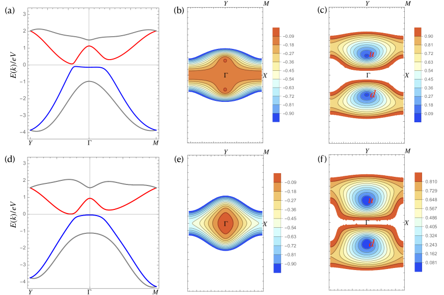
Figure 4: (a)-(c), band structure of monolayer WTe₂ from the tight binding model in Ref.[83]. The energy dispersion along a particular trajectory $Y$-$\Gamma$-$M$ is shown in (a), the energy contours for the valence band and conduction band are shown in (b) and (c) respectively. (d)-(f), band structure of monolayer WTe₂ from the tight binding model in Ref.[84]. The energy dispersion along a particular trajectory $Y$-$\Gamma$-$M$ is shown in (d), the energy contours for the valence band and conduction band are shown in (e) and (f) respectively. The conduction band for these two models are quite similar. For the valence band, the model in Ref.[83] indicates that the band top is shifted away from $\Gamma$ point, while the valence band top obtained from the model in Ref.[84] is still at $\Gamma$ point. This difference will have huge impact on the hole-doped moiré bands, which are constructed using the valence band dispersion. For the conduction band, both models contain two separated electron pockets which we dub as ‘u’ and ‘d’ fermions, and therefore the resulting electron-doped moiré bands from these two models are similar.

The second tight-binding model (model II) is proposed in Ref. [84], which we also copy for convenience here. The first term is $H_{0}s_{0}$ where

$$H_{0} =[\frac{\mu_{p}}{2}+t_{px}\cos(ak_{x})+t_{py}\cos(bk_{y})]\Gamma_{1}^{-}+[\frac{\mu_{d}}{2}+t_{dx}\cos(ak_{x})]\Gamma_{1}^{+}$$ (13)

$$+ t_{dAB}e^{-ibk_{y}}(1+e^{iak_{x}})e^{i\bm{k}\cdot\Delta_{1}}\Gamma_{2}^{+}+t_{pAB}(1+e^{iak_{x}})e^{i\bm{k}\cdot\Delta_{2}}\Gamma_{2}^{-}+t_{0AB}(1-e^{iak_{x}})e^{i\bm{k}\cdot\Delta_{3}}\Gamma_{3}$$

$$- 2it_{0x}\sin(ak_{x})[e^{i\bm{k}\cdot\Delta_{4}}\Gamma_{4}^{+}+e^{-i\bm{k}\cdot\Delta_{4}}\Gamma_{4}^{-}]+t_{0ABx}(e^{-iak_{x}}-e^{2iak_{x}})e^{i\bm{k}\cdot\Delta_{3}}\Gamma_{3}+\text{h.c.}$$

The SOC part is

$$H_{soc} =[(\lambda_{dx}^{z}s_{z}+\lambda_{dx}^{y}s_{y})\sin(ak_{x})]\Gamma_{5}^{+}+[(\lambda_{px}^{z}s_{z}+\lambda_{px}^{y}s_{y})\sin(ak_{x})]\Gamma_{5}^{-}$$ (14)

$$- i\lambda_{0AB}^{y}s_{y}(1+e^{iak_{x}})e^{i\bm{k}\cdot\Delta_{3}}\Gamma_{6}-i(\lambda_{0}^{z}s_{z}+\lambda_{0}^{y}s_{y})(e^{i\bm{k}\cdot\Delta_{4}}{\Gamma_{4}^{+}}-e^{-i\bm{k}\cdot\Delta_{4}}\Gamma_{4}^{-})$$

$$- i(\lambda^{{}^{\prime}z}_{0}s_{z}+\lambda_{0}^{{}^{\prime}y}s_{y})(e^{-ibk_{y}}e^{i\bm{k}\cdot\Delta_{4}}\Gamma^{+}-e^{ibk_{y}}e^{-i\bm{k}\cdot\Delta_{4}}\Gamma^{-})+\text{h.c.}$$

Here $a=3.477$Å and $b=6.249$Å. $\Delta_{1}=\bm{r}_{Ad}-\bm{r}_{Bd}$, $\Delta_{2}=\bm{r}_{Ap}-\bm{r}_{Bp}$, $\Delta_{3}=\bm{r}_{Ad}-\bm{r}_{Bp}$ and $\Delta_{4}=\bm{r}_{Ad}-\bm{r}_{Ap}$, with $\bm{r}_{Ad}=(-0.25a,0.32b)$, $\bm{r}_{Bp}=(0.25a,0.07b)$, $\bm{r}_{Ap}=(-0.25a,-0.07b)$ and $\bm{r}_{Bd}=(0.25a,-0.32b)$. The $\Gamma$ matrices are defined as

$$\Gamma_{0} =\sigma_{0}l_{0},~{}\Gamma_{1}^{\pm}=\frac{\sigma_{0}}{2}(l_{0}\pm l_{3}),~{}\Gamma_{2}^{\pm}=\frac{1}{4}(\sigma_{1}+i\sigma_{2})(l_{0}\pm l_{3}),~{}\Gamma_{3}=\frac{1}{2}(\sigma_{1}+i\sigma_{2})il_{2}$$ (15)

$$\Gamma_{4}^{\pm} =\frac{1}{4}(\sigma_{0}\pm\sigma_{3})(l_{1}+il_{2}),~{}\Gamma_{5}^{\pm}=\frac{\sigma_{3}}{2}(l_{0}\pm l_{3}),~{}\Gamma_{6}=\frac{1}{2}(\sigma_{1}+i\sigma_{2})l_{1}.$$

And the parameters are

$$\mu_{p}=-1.75,~{}~{}~{} \lambda_{0AB}^{y}=0.011{}{}{} \mu_{d}=0.74,~{}~{}~{} \lambda_{0}^{y}=0.051$$ (16)

$$t_{px}=1.13,~{}~{}~{} \lambda_{0}^{z}=0.012{}{}{} t_{dx}=-0.41,~{}~{}~{} \lambda_{0}^{{}^{\prime}y}=0.05$$

$$t_{pAB}=0.4,~{}~{}~{} \lambda_{0}^{{}^{\prime}z}=0.012{}{}{} t_{dAB}=0.51,~{}~{}~{} \lambda_{px}^{y}=-0.04$$

$$t_{0AB}=0.39,~{}~{}~{} \lambda_{px}^{z}=-0.01{}{}{} t_{0ABx}=0.29,~{}~{}~{} \lambda_{dx}^{y}=-0.031$$

$$t_{0x}=0.14,~{}~{}~{} \lambda_{dx}^{z}=-0.008{}{}{} t_{py}=0.13$$

In Fig. 4(d)-(f) we show the band structure and the constant energy contours obtained from model II. Note in this model, the valence band top is at $\Gamma$ point, which is consistent with the DFT calculations in Ref. [83], and is also consistent with the ARPES data in Ref. [85]. For the electron-doped monolayer, there are two electron-pockets located along $\Gamma$-Y line, which agrees with model I and justifies our division of low energy fermions into ‘u’ and ‘d’ sectors related by $C_{2z}$ rotation.

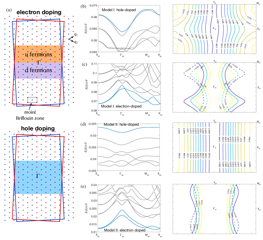
Figure 5: Emergence of quasi-1D moiré band structure from twisted bilayer WTe₂, obtained from both model I and model II using $w=5$meV and $\theta=2.12^{\circ}$. (a) Cutoff procedure for constructing the moiré band structures from the tight banding models. For electron-doped tWTe₂, since the low energy fermions are located in two separate positions, we divide the monolayer Brillouin zone into two part which we call u- and d-fermions. Moiré bands in this case are obtained using u- and d-fermions separately, assuming the coupling between them is negligible. For hole-doped tWTe₂, we use the band fermions inside the blue region as a whole to construct moiré bands. (b) Band structure for hole-doped tWTe₂ based on the model I [83]. The first two bands are energetically close to each other, which is due to the fact that in model I there are two maxima for the valence band. The right panel shows energy contours for the topmost moiré band. (c) Band structure for electron-doped tWTe₂ based on the model I. The two bottom bands are energetically close to each other, which are from u- and d-fermions. The right panel shows energy contours for the bottommost moiré bands. (d) Band structure for hole-doped tWTe₂ based on the model II [84]. Note there is only one topmost moiré band. The right panel shows energy contours for the topmost moiré band. (c) Band structure for electron-doped tWTe₂ based on the model II. The two bottom bands are energetically close to each other, which are from u- and d-fermions. The right panel shows energy contours for the bottommost moiré bands.

We now discuss the band structures for twisted bilayer WTe₂, using the continuum model analogous to the twisted bilayer graphene [93] and other twisted bilayer TMD [57, 58] systems. In practice, we need to distinguish between electron doped and hole doped tWTe₂, this is because for the hole-doped system, the low energy fermions are from the hole pocket centered at $\Gamma$ point, but for electron-doped system the low energy fermions are from both u- and d-pockets. If we neglect the coupling between u and d fermions, we can use each of the electron pocket to construct moiré band individually, then the resulting moiré band fermions acquire additional pseudospin indices $\tau=$u,d, and the particle number for u and d fermions are individually conserved, and $\tau=$u,d effectively becomes a good quantum numbers in addition to the physical spin. In Fig. 5(a) we show the momentum cutoff procedures when constructing the moiré bands. For hole-doped systems, we consider a large region centered at the $\Gamma$ point, while for electron doped systems, we separately consider two regions centered at either u- or d-pockets.

Let’s discuss the electron-doped system for instance. The continuum limit Hamiltonian in this case can be written as (for each spin projection)

$$H_{\tau}=\begin{pmatrix}\varepsilon_{\tau,t}(\bm{k})&T(\bm{r})\\ T^{\dagger}(\bm{r})&\varepsilon_{\tau,b}(\bm{k}).\end{pmatrix}$$ (17)

where $\epsilon_{\tau,t/b}(\bm{k})$ is the monolayer band dispersion rotated by $\theta/2$ and $-\theta/2$. Technically, this can be obtained by first diagonalizing the tight binding Hamiltonian and rotating by $\pm\theta/2$ on a meshgrid, and then using numerical interpolation to obtain energies at arbitrary $\bm{k}$. The interlayer coupling $T(\bm{r})=2w[\cos(\bm{q}_{1}\cdot\bm{r})+\cos(\bm{q}_{2}\cdot\bm{r})]$ where the two vectors $\bm{q}_{1}$ and $\bm{q}_{2}$ are shown in Fig. 5(a) and $w$ is the interlayer tunneling strength. As is also shown in Fig. 5(a), we divide the momentum space into two parts by setting some momentum cutoff: the orange region containing u fermions is used for construction of $H_{\text{u}}$, while the purple region contains d fermions and is used for $H_{\text{d}}$. We also choose some specific twist angles such that the width of the original Brillouin zone is approximately integer multiples of the length of the resulting moiré Brillouin zone.

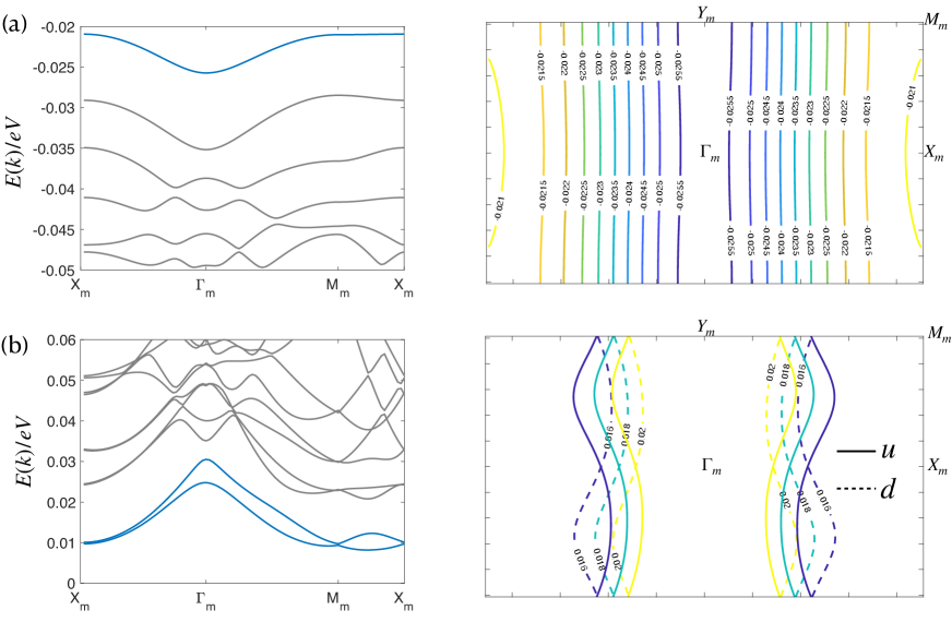
Figure 6: Moiré band structure obtained from model II at $\theta=2.89$ and $w=8$mEV for (a) hole-doping and (b) electron-doping.

In Fig. 5(b-e) we present the moiré band structure and constant energy contours for the first moiré band calculated from both model I and model II. Here we have chosen $w=5$meV and $\theta=2.12^{\circ}$. We note the precise value of $w$ does not lead to any qualitative difference and other choices of $w$ of the same order yields similar results. The hole-doped moiré bands obtained from model I is shown in Fig. 5(b). The first two (top) bands are energetically close to each other, a direct consequence of the fact that model I has two valence band maximums located along $\Gamma$-Y line. But as we noted above, this behavior is not consistent with DFT and ARPES results. The electron-doped moiré bands obtained from model I is shown in Fig. 5(c). The first two moiré bands are highlighted in blue, and the corresponding constant energy contours shows that u- and d-fermions are indeed related by $C_{2z}$ rotation. The same moiré bands obtained from model II are shown in Fig. 5(d) and (c). For the hole-doped bands, we see that the first two bands are well separated in energy scale, which is consistent with the fact that in model II the valence band maximum is unique and located at $\Gamma$. The electron doped moiré bands are similar to those obtained from model I, which also reflects the $C_{2z}$ symmetry relation between u- and d-fermions. This symmetry can also be seen at the Hamiltonian level. Since we have $\varepsilon_{\text{u},t}(\bm{k})=\varepsilon_{\text{d},t}(-\bm{k})$ ($\bm{k}$ here is measured from $\Gamma$ point) and $T(\bm{r})$ is invariant under inversion,

$$H_{\text{u}}(\bm{k})\leftrightarrow H_{\text{d}}(-\bm{k})$$ (18)

under the inversion operation. This indicates the resulting moiré band structure also has this relation $E_{\text{u}}(\bm{k})=E_{\text{d}}(-\bm{k})$.

From the above comparison, we believe model II is more faithful in representing the low energy band structures of WTe₂. In Fig. 6 we shown additional results of both hole-doped and electron-doped moiré bands obtained from model II with $w=8$meV and a larger twist angle $\theta=2.89^{\circ}$. The moiré bands in this case are quite similar to those obtained at $\theta=2.12^{\circ}$. Again we can clearly see the hole-doped side is more quasi-1D, but the electron-doped side has additional pseudo-spin flavor.

II II. Bosonization of the Multi-component 1D system

As discussed in the main text and in the above section that we model the decoupled 1D wire system with multi components labeled by $\lambda=(s_{z},\tau_{z})$, where $s_{z}=\uparrow,\downarrow$ is the physical spin and $\tau_{z}=\text{u,d}$ is Fermi line index. The spin degeneracy ensures that the spin-up fermions and spin-down fermions have the same Fermi momentum $k_{F}$. Furthermore, according to the inversion symmetry between u and d fermions discussed above, the u and d fermions should also have the same $k_{F}$ if we require each wire to respect this inversion symmetry. For simplicity, we also assume that $k_{F}$ is incommensurate so we neglect Umklapp scattering. The total Hamiltonian for each wire can be written as

$$H_{1D}=H_{0}+H_{I}$$ (19)

where

$$H_{0}=\sum_{k,r,\lambda}v_{F}(rk-k_{F})\psi_{r,\lambda}^{\dagger}(k)\psi_{r,\lambda}(k)=2\pi v_{F}\sum_{q>0,r,\lambda}\rho_{r,\lambda}(q)\rho_{r,\lambda}(-q)$$ (20)

Here $L$ is the wire length, $v_{F}$ is the Fermi velocity and $r=\pm$ denotes right ($+$) and left ($-$) movers. The momentum summation is $\sum_{q}\equiv\frac{1}{L}\sum_{q}$. The interaction part is written as (assuming short range interaction)

$$H_{I} =\frac{1}{L}\sum_{k,p,q}\sum_{\lambda\neq\lambda^{\prime}}V_{1,\lambda\lambda^{\prime}}\psi^{\dagger}_{+,\lambda}(k)\psi^{\dagger}_{-,\lambda^{\prime}}(p)\psi_{+,\lambda^{\prime}}(p+q)\psi_{-,\lambda}(k-q)$$ (21)

$$+\frac{1}{L}\sum_{k,p,q}\sum_{r,\lambda=\lambda^{\prime}}V_{1,\lambda\lambda^{\prime}}\psi^{\dagger}_{r,\lambda}(k)\psi^{\dagger}_{-r,\lambda^{\prime}}(p)\psi_{r,\lambda^{\prime}}(p+q)\psi_{-r,\lambda}(k-q)$$

$$+\frac{1}{L}\sum_{q,r,\lambda,\lambda^{\prime}}V_{2,\lambda\lambda^{\prime}}\rho_{r,\lambda}(q)\rho_{-r,\lambda^{\prime}}(-q)+\frac{1}{L}\sum_{r,q,\lambda.\lambda^{\prime}}V_{4,\lambda\lambda^{\prime}}\rho_{r,\lambda}(q)\rho_{r,\lambda^{\prime}}(-q).$$

Here we have adopted the notations from previous literatures such that $V_{1}$ is for backscatterting, and $V_{2}$ and $V_{4}$ are two forward scatterings. We assume the system is away from commensurate filling such that $4k_{F}$ is not a reciprocal lattice vector, so we neglect the umklapp scattering $V_{3}$. In analogy to two-component 1D systems, it will be convenient to further distinguish $V_{i,\lambda\lambda}$ according to different spin and orbit configurations. To this end, we define,

$$V_{i,\lambda\lambda^{\prime}}=V_{i,1},~{}~{}~{}\text{if}~{}~{}s_{z}=s_{z}^{\prime},~{}\tau_{z}=\tau_{z}^{\prime};$$ (22)

$$V_{i,\lambda\lambda^{\prime}}=V_{i,2},~{}~{}~{}\text{if}~{}~{}s_{z}\neq s_{z}^{\prime},~{}\tau_{z}=\tau_{z}^{\prime};$$

$$V_{i,\lambda\lambda^{\prime}}=V_{i,3},~{}~{}~{}\text{if}~{}~{}s_{z}=s_{z}^{\prime},~{}\tau_{z}\neq\tau_{z}^{\prime};$$

$$V_{i,\lambda\lambda^{\prime}}=V_{i,4},~{}~{}~{}\text{if}~{}~{}s_{z}\neq s_{z}^{\prime},~{}\tau_{z}\neq\tau_{z}^{\prime}.$$

Like the the spin and charge densities in conventional 1DEG, for the four-component system it’s useful to define the following four chiral-densities,

$$\rho_{0} =\frac{1}{2}\left(\rho_{\uparrow\text{u}}+\rho_{\downarrow\text{u}}+\rho_{\uparrow\text{d}}+\rho_{\downarrow\text{d}}\right),$$ (23)

$$\rho_{1} =\frac{1}{2}\left(\rho_{\uparrow\text{u}}-\rho_{\downarrow\text{u}}+\rho_{\uparrow\text{d}}-\rho_{\downarrow\text{d}}\right),$$

$$\rho_{2} =\frac{1}{2}\left(\rho_{\uparrow\text{u}}+\rho_{\downarrow\text{u}}-\rho_{\uparrow\text{d}}-\rho_{\downarrow\text{d}}\right),$$

$$\rho_{3} =\frac{1}{2}\left(\rho_{\uparrow\text{u}}-\rho_{\downarrow\text{u}}-\rho_{\uparrow\text{d}}+\rho_{\downarrow\text{d}}\right),$$

where the $r$-index is omitted for brevity. Using Eq.(22) and (23), we can rewrite $H_{0}$, the two forward-scattering terms ($V_{2}$ and $V_{4}$) and the backward-scattering with $\lambda=\lambda^{\prime}$ ($V_{1,1}$) in $H_{I}$ as

$$\sum_{q} [(V_{2,1}-V_{1,1})(\rho_{r,0}\rho_{-r,0}+\rho_{r,1}\rho_{-r,1}+\rho_{r,2}\rho_{-r,2}+\rho_{r,3}\rho_{-r,3})+V_{2,2}(\rho_{r,0}\rho_{-r,0}-\rho_{r,1}\rho_{-r,1}+\rho_{r,2}\rho_{-r,2}-\rho_{r,3}\rho_{-r,3})$$ (24)

$$+ V_{2,3}(\rho_{r,0}\rho_{-r,0}+\rho_{r,1}\rho_{-r,1}-\rho_{r,2}\rho_{-r,2}-\rho_{r,3}\rho_{-r,3})+V_{2,4}(\rho_{r,0}\rho_{-r,0}-\rho_{r,1}\rho_{-r,1}-\rho_{r,2}\rho_{-r,2}+\rho_{r,3}\rho_{-r,3})]$$

$$+\sum_{r,q} [(\pi v_{F}+V_{4,1})(\rho_{r,0}^{2}+\rho_{r,1}^{2}+\rho_{r,2}^{2}+\rho_{r,3}^{2})+V_{4,2}(\rho_{r,0}^{2}-\rho_{r,1}^{2}+\rho_{r,2}^{2}-\rho_{r,3}^{2})$$

$$+ V_{4,3}(\rho_{r,0}^{2}+\rho_{r,1}^{2}-\rho_{r,2}^{2}-\rho_{r,3}^{2})+V_{4,4}(\rho_{r,0}^{2}-\rho_{r,1}^{2}-\rho_{r,2}^{2}+\rho_{r,3}^{2})].$$

The other backward-scattering terms are cast into cosine terms by introducing the following bosonization formula,

$$\psi_{r,\lambda}(x)=\lim_{\alpha\to 0}\frac{U_{r,\lambda}}{\sqrt{2\pi\alpha}}\exp\left[i\theta_{\lambda}(x)+ir(k_{F}x-\phi_{\lambda}(x))\right]$$ (25)

where $\alpha$ is a UV cutoff and $U_{r,\lambda}$ are the Klein factors. It’s also convenient at this point to introduce $\phi_{i}$ in terms of $\phi_{\lambda}$, completely parallel to Eq.(23),

$$\phi_{0} =\frac{1}{2}\left(\phi_{\uparrow\text{u}}+\phi_{\downarrow\text{u}}+\phi_{\uparrow\text{d}}+\phi_{\downarrow\text{d}}\right),$$ (26)

$$\phi_{1} =\frac{1}{2}\left(\phi_{\uparrow\text{u}}-\phi_{\downarrow\text{u}}+\phi_{\uparrow\text{d}}-\phi_{\downarrow\text{d}}\right),$$

$$\phi_{2} =\frac{1}{2}\left(\phi_{\uparrow\text{u}}+\phi_{\downarrow\text{u}}-\phi_{\uparrow\text{d}}-\phi_{\downarrow\text{d}}\right),$$

$$\phi_{3} =\frac{1}{2}\left(\phi_{\uparrow\text{u}}-\phi_{\downarrow\text{u}}-\phi_{\uparrow\text{d}}+\phi_{\downarrow\text{d}}\right).$$

The inverse relations are

$$\phi_{\uparrow\text{u}} =\frac{1}{2}\left(\phi_{0}+\phi_{1}+\phi_{2}+\phi_{3}\right),$$ (27)

$$\phi_{\downarrow\text{u}} =\frac{1}{2}\left(\phi_{0}-\phi_{1}+\phi_{2}-\phi_{3}\right),$$

$$\phi_{\uparrow\text{d}} =\frac{1}{2}\left(\phi_{0}+\phi_{1}-\phi_{2}-\phi_{3}\right),$$

$$\phi_{\downarrow\text{d}} =\frac{1}{2}\left(\phi_{0}-\phi_{1}-\phi_{2}+\phi_{3}\right).$$

Using this relation, it is straightforward to rewrite the back-scattering terms as

$$\frac{V_{1,2}}{(2\pi\alpha)^{2}}\int dx\left\{U^{\dagger}_{R\uparrow u}U^{\dagger}_{L\downarrow u}U_{R\downarrow u}U_{L\uparrow u}e^{i2(\phi_{2}+\phi_{4})}+sU^{\dagger}_{R\uparrow d}U^{\dagger}_{L\downarrow d}U_{R\downarrow d}U_{L\uparrow d}e^{i2(\phi_{2}-\phi_{4})}+\text{h.c.}\right\}$$ (28)

$$+ \frac{V_{1,3}}{(2\pi\alpha)^{2}}\int dx\left\{U^{\dagger}_{R\uparrow u}U^{\dagger}_{L\uparrow d}U_{R\uparrow d}U_{L\uparrow u}e^{i2(\phi_{3}+\phi_{4})}+sU^{\dagger}_{R\downarrow u}U^{\dagger}_{L\downarrow d}U_{R\downarrow d}U_{L\downarrow u}e^{i2(\phi_{3}-\phi_{4})}+\text{h.c.}\right\}$$

$$+ \frac{V_{1,4}}{(2\pi\alpha)^{2}}\int dx\left\{U^{\dagger}_{R\uparrow u}U^{\dagger}_{L\downarrow d}U_{R\downarrow d}U_{L\uparrow u}e^{i2(\phi_{2}+\phi_{3})}+sU^{\dagger}_{R\uparrow d}U^{\dagger}_{L\downarrow u}U_{R\downarrow u}U_{L\uparrow d}e^{i2(\phi_{2}-\phi_{3})}+\text{h.c.}\right\}$$

These Klein factors in thermodynamic limit can be replaced by Majorana fermion operators, given that their change on the particle number can be neglected. So we will introduce $R_{\lambda}$ and $L_{\lambda}$ to denote the Majoranas which satisfy $R_{\lambda}R_{\lambda}=L_{\lambda}L_{\lambda}=1$. They are important in order to properly identify the order parameters, as we will see in the next section. At this point, we need to use them to determine $s$. The strategy is to come up with some auxiliary order parameter, for instance (the boson parts are omitted),

$$R_{\uparrow u}L_{\downarrow u}R_{\downarrow u}L_{\uparrow u}+sR_{\uparrow d}L_{\downarrow d}R_{\downarrow d}L_{\uparrow d}$$ (29)

$$+ R_{\uparrow u}L_{\uparrow d}R_{\uparrow d}L_{\uparrow u}+sR_{\downarrow d}L_{\downarrow u}R_{\downarrow u}L_{\downarrow d}.$$

Suppose we evaluate this operator perturbatively in the presence of $V_{1,4}$, so we need to expand $e^{-\beta H_{I}}$ to the first order of $V_{1,4}$. In order to maintain the form of the order parameter, we need to set $s=-1$. As a result, the bosonized form of the interactions is given by

$$-\frac{4V_{1,2}}{(2\pi\alpha)^{2}}\int dx\sin(2\phi_{1})\sin(2\phi_{3})-\frac{4V_{1,3}}{(2\pi\alpha)^{2}}\int dx\sin(2\phi_{2})\sin(2\phi_{3})-\frac{4V_{1,4}}{(2\pi\alpha)^{2}}\int dx\sin(2\phi_{1})\sin(2\phi_{2}).$$ (30)

Note in the main text we have introduced new definitions for these backscattering terms as follows,

$$g_{2}:=V_{1,2},~{}~{}g_{1}:=V_{1,3},~{}~{}g_{3}:=V_{1,4}.$$ (31)

Alternatively, we can use $-V_{1,2}$, $-V_{1,3}$ and $-V_{1,4}$ in Eq.(28), and similar reasoning leads to $s=1$ instead. Therefore in this convention the interaction is given by

$$-\frac{4g_{2}}{(2\pi\alpha)^{2}}\int dx\cos(2\phi_{1})\cos(2\phi_{3})-\frac{4g_{1}}{(2\pi\alpha)^{2}}\int dx\cos(2\phi_{2})\cos(2\phi_{3})-\frac{4g_{3}}{(2\pi\alpha)^{2}}\int dx\cos(2\phi_{1})\cos(2\phi_{2}),$$ (32)

where we have used the new convention defined in Eq.(31).

The field $\phi_{i}$ is related to $\rho_{i}$ as follows

$$-\frac{1}{\pi}\partial_{x}\phi_{i}(x)=\rho_{+,i}(x)+\rho_{-,i}(x)-\rho_{0,i}.$$ (33)

where $\rho_{0}$ is the average density. So we can identify

$$\text{Charge density fluctuations}:~{}\frac{1}{\pi}\partial_{x}\phi_{0}(x), ~{}~{}~{}~{}\text{Spin density fluctuations}:~{}\frac{1}{\pi}\partial_{x}\phi_{1}(x),$$ (34)

$$\text{Valley density fluctuations}:~{}\frac{1}{\pi}\partial_{x}\phi_{2}(x), ~{}~{}~{}~{}\text{Spin-valley density fluctuations}:~{}\frac{1}{\pi}\partial_{x}\phi_{3}(x).$$

The conjugate field $\Pi_{i}$ is

$$\Pi_{i}(x)=\rho_{+,i}(x)-\rho_{-,i}(x).$$ (35)

It is related to the $\theta(x)$ in Eq.(25) via

$$\Pi_{i}(x)=\frac{1}{\pi}\partial_{x}\theta(x).$$ (36)

Expressing the fermion density operators in terms of $\Pi_{i}(x)$ and $\phi_{i}(x)$ we have,

$${}^{2}+[\rho_{-,i}(x)]^{2} =\frac{[\frac{1}{\pi}\partial_{x}\phi_{i}(x)-\rho_{0,i}]^{2}+[\Pi_{i}(x)]^{2}}{2}$$ (37)

$$\rho_{+,i}(x)\rho_{-,i}(x)+\rho_{-,i}(x)\rho_{+,i}(x) =\frac{[\frac{1}{\pi}\partial_{x}\phi_{i}(x)-\rho_{0,i}]^{2}-[\Pi_{i}(x)]^{2}}{2}.$$

Substituting these relations to Eq.(24) and combining it with Eq.(32), we arrive at the final bosonized Hamiltonian (up to some constant)

$$H= \sum_{i=0}^{3}\int dx\left\{\frac{\pi v_{i}K_{i}}{2}\left[\Pi_{i}(x)\right]^{2}+\frac{v_{i}}{2\pi K_{i}}\left[\partial_{x}\phi_{i}(x)\right]^{2}\right\}$$ (38)

$$-\frac{4g_{2}}{(2\pi\alpha)^{2}}\int dx\cos(2\phi_{1})\cos(2\phi_{3})-\frac{4g_{1}}{(2\pi\alpha)^{2}}\int dx\cos(2\phi_{2})\cos(2\phi_{3})-\frac{4g_{3}}{(2\pi\alpha)^{2}}\int dx\cos(2\phi_{1})\cos(2\phi_{2}),$$

where $\phi_{i}\equiv\phi_{i}(x)$ and the renormalized velocities $u_{i}$ and Luttinger parameters $K_{i}$ are given by

$$v_{i}=\sqrt{(v_{F}+G_{i}/\pi)(v_{F}+U_{i}/\pi)},~{}~{}K_{i}=\sqrt{\frac{\pi v_{F}+U_{i}}{\pi v_{F}+G_{i}}}.$$ (39)

Here $U_{i}$ and $G_{i}$ are determined by $V_{i,j}$:

$$V_{0}=V_{4,1}+V_{4,2}+V_{4,3}+V_{4,4}+V_{2,1}-V_{1,1}+V_{2,2}+V_{2,3}+V_{2,4},$$ (40)

$$U_{0}=V_{4,1}+V_{4,2}+V_{4,3}+V_{4,4}-V_{2,1}+V_{1,1}-V_{2,2}-V_{2,3}-V_{2,4},$$

$$V_{1}=V_{4,1}-V_{4,2}+V_{4,3}-V_{4,4}+V_{2,1}-V_{1,1}-V_{2,2}+V_{2,3}-V_{2,4},$$

$$U_{1}=V_{4,1}-V_{4,2}+V_{4,3}-V_{4,4}-V_{2,1}+V_{1,1}+V_{2,2}-V_{2,3}+V_{2,4},$$

$$V_{2}=V_{4,1}+V_{4,2}-V_{4,3}-V_{4,4}+V_{2,1}-V_{1,1}+V_{2,2}-V_{2,3}-V_{2,4},$$

$$U_{2}=V_{4,1}+V_{4,2}-V_{4,3}-V_{4,4}-V_{2,1}+V_{1,1}-V_{2,2}+V_{2,3}+V_{2,4},$$

$$V_{3}=V_{4,1}-V_{4,2}-V_{4,3}+V_{4,4}+V_{2,1}-V_{1,1}-V_{2,2}-V_{2,3}+V_{2,4},$$

$$U_{3}=V_{4,1}-V_{4,2}-V_{4,3}+V_{4,4}-V_{2,1}+V_{1,1}+V_{2,2}+V_{2,3}-V_{2,4}.$$

In a special case when all $V_{i,j}=V_{i,j^{\prime}}\equiv V_{i}$ for every $i$, $j$ and $j^{\prime}$, and neglecting the backscattering term $V_{1,i}$, we obtain

$$G_{0}=4(V_{4}+V_{2}),~{}~{}U_{0}=4(V_{4}-V_{2}),$$ (41)

$$G_{1}=U_{1}=G_{2}=U_{2}=G_{3}=U_{3}=0.$$

Then it is easy to see from Eq.(39) that $v_{1}=v_{2}=v_{3}=v_{F}$ and $K_{1}=K_{2}=K_{3}=1$. When the backscattering is included, as we will see below that for repulsive interaction, the system still flows to this fixed point, while for attraction, the system tends to gap opening.

Without the backscattering (cosine) terms, Eq.(38) remains unchanged via

$$\theta_{i}(x)\leftrightarrow\phi_{i}(x)~{}~{}\text{and}~{}~{}K_{i}\leftrightarrow\frac{1}{K_{i}}$$ (42)

which is called T-duality. This observation will be used later to evaluate the correlation functions.

The Hamiltonian in Eq.(38) leads to the following action:

$$S_{tot}=\sum_{i=0}^{3}S_{i}+S_{I}$$ (43)

where

$$S_{i} =\frac{1}{2\pi K_{i}}\int dxd\tau\left\{\frac{1}{v_{i}}\left(\partial_{\tau}\phi_{i}\right)^{2}+v_{i}\left(\partial_{x}\phi_{i}\right)^{2}\right\}$$ (44)

$$=\frac{1}{2\pi K_{i}}\int dxdy\left\{\tilde{v}_{i}\left(\partial_{x}\phi_{i}\right)^{2}+\frac{1}{\tilde{v}_{i}}\left(\partial_{y}\phi_{i}\right)^{2}\right\}$$

with $y:=\bar{v}\tau$ and $\tilde{v}_{i}=v_{i}/\bar{v}$ with $\bar{v}=(v_{1}+v_{2}+v_{3})/3$. The integration limits will be the same in zero temperature limit. Similarly,

$$S_{I}=-\frac{4}{(2\pi\alpha)^{2}}\int d^{2}\bm{r}\left[\frac{g_{2}}{\bar{v}}\cos(2\phi_{1})\cos(2\phi_{3})+\frac{g_{1}}{\bar{v}}\cos(2\phi_{2})\cos(2\phi_{3})+\frac{g_{3}}{\bar{v}}\cos(2\phi_{1})\cos(2\phi_{2})\right].$$ (45)

Without the cosine terms, the regularized Green’s function is given by

$$G(x,t):=\braket{\phi_{j}(x,t)\phi_{j}(0,0)}=-\frac{K_{j}}{4}\ln\left[\frac{x^{2}+y^{2}+a^{2}}{R^{2}}\right]_{y\to iv_{j}t+a}=-\frac{K_{j}}{4}\ln\left[\frac{x^{2}+(iv_{j}t+a)^{2}}{R^{2}}\right]$$ (46)

where $a\to 0$ and $R\to\infty$ are the UV and IR cutoff respectively. According to the T-duality we have

$$G_{\theta\theta}(x,t):=\braket{\theta_{j}(x,t)\theta_{j}(0,0)}=-\frac{1}{4K_{j}}\ln\left[\frac{x^{2}+(iv_{j}t+a)^{2}}{R^{2}}\right].$$ (47)

The Green’s function between $\phi_{j}$ field and $\theta_{j}$ field is calculated from the original action when both of these two fields are present,

$$G_{\phi\theta}(x,t):=\braket{\phi_{j}(x,t)\theta_{j}(0,0)}=-\frac{1}{4}\ln\frac{i(v_{j}t+x)+a}{i(v_{j}t-x)+a}.$$ (48)

On the other hand, if the boson becomes massive, namely

$$S_{i}=\frac{1}{2\pi K_{i}}\int dxdy\left\{\left(\partial_{x}\phi_{i}\right)^{2}+\left(\partial_{y}\phi_{i}\right)^{2}+m^{2}\phi_{i}^{2}\right\},$$ (49)

then the correlation function is given by

$$\braket{\phi_{i}(\bm{r})\phi_{i}(0)}=\frac{K_{i}}{2}K_{0}(m|\bm{r}|)$$ (50)

where $K_{0}(...)$ is the modified Bessel function of the second kind, which decays exponentially at large distance,

$$K_{0}(m|\bm{r}|)\sim e^{-m|\bm{r}|}.$$ (51)

and behaves as logarithmic at short distances

$$K_{0}(m|\bm{r}|)\sim-\frac{1}{2}\ln(m^{2}\bm{r}^{2}).$$ (52)

Therefore, we can identify the correlation length as $\xi=1/m$ which is finite. The correlation function in space-time coordinates in the massive case is thus

$$G(x,t)=\frac{K_{j}}{2}K_{0}\left(\frac{\sqrt{x^{2}+(iv_{j}t+a)^{2}}}{\xi}\right).$$ (53)

III III. Order parameters and correlation functions at Gaussian fixed point

To obtain the correlation functions, one can make use of the general formula for the vertex operator correlation functions for a massless boson model (let’s at this point neglect the logarithmic corrections due to finite backscattering in the limit when all $K_{i}\to 1$),

$$\braket{e^{i\beta_{1}\phi(\bm{r}_{1})}...e^{i\beta_{N}\phi(\bm{r}_{N})}} =\exp\left(-\sum_{i>j}\beta_{i}\beta_{j}G(\bm{r}_{i},\bm{r}_{j})\right)\exp\left(-\frac{1}{2}\sum_{i}\beta_{i}^{2}G(\bm{r}_{i},\bm{r}_{i})\right)$$ (54)

This equation can be proved by using the cumulant expansion formula for Gaussian action.

III.1 Massless boson

If the boson model is massless, we expect that the expectation value of the vertex operator vanishes. This is because

$$\braket{e^{i\beta\phi_{j}(x)}}=\exp\left[-\frac{1}{2}\beta^{2}G(0)\right]=\left(\frac{a}{R}\right)^{\frac{\beta^{2}K_{j}}{4}},$$ (55)

where $G(0)$ is the Green’s function in Eq.(46) in the IR limit. Apparently, this results vanishes in the limit when $R\to\infty$. This results is consistent with the fact that in the massless case the expectation value of order paramters remains zero.

For multi-point correlation functions, we use the explicit formula for the Green’s function in Eq.(46) in the massless case and obtain

$$\braket{e^{i\beta_{1}\phi(\bm{r}_{1})}...e^{i\beta_{N}\phi(\bm{r}_{N})}} =\prod_{i>j}\left[\frac{(x_{i}-x_{j})^{2}+(y_{i}-y_{j})^{2}+a^{2}}{R^{2}}\right]^{\frac{\beta_{i}\beta_{j}K}{4}}\prod_{i}\left[\frac{a^{2}}{R^{2}}\right]^{\frac{\beta_{i}^{2}K}{8}}$$ (56)

$$=\prod_{i>j}\left[\frac{(x_{i}-x_{j})^{2}+(y_{i}-y_{j})^{2}+a^{2}}{a^{2}}\right]^{\frac{\beta_{i}\beta_{j}K}{4}}\left[\frac{a}{R}\right]^{\frac{K}{8}(\sum_{i}\beta_{i})^{2}}.$$

The correlation function does not vanish in the limit $R\to\infty$ only if $\sum_{i}\beta_{i}=0$. From this general expression for correlations functions, it is easy to obtain

$$\braket{e^{i\phi_{j}(x,t)-i\phi_{j}(0)}} =\left(\frac{a^{2}}{x^{2}+(iv_{j}t+a)^{2}}\right)^{\frac{K_{j}}{4}},$$ (57)

$$\braket{\cos\phi_{j}(x,t)\cos\phi_{j}(0,0)} =\braket{\sin\phi_{j}(x,t)\sin\phi_{j}(0,0)}=\frac{1}{2}\left(\frac{a^{2}}{x^{2}+(iv_{j}t+a)^{2}}\right)^{\frac{K_{j}}{4}},$$

$$\braket{\cos\phi_{j}(x,t)\sin\phi_{j}(0,0)} =\braket{\sin\phi_{j}(x,t)\cos\phi_{j}(0,0)}=0.$$

The correlation functions for the $\theta$ field can be found by the duality relation in Eq.(42).

$$\braket{e^{i\theta_{j}(x,t)-i\theta_{j}(0)}} =\left(\frac{a^{2}}{x^{2}+(iv_{j}t+a)^{2}}\right)^{\frac{1}{4K_{j}}},$$ (58)

$$\braket{\cos\theta_{j}(x,t)\cos\theta_{j}(0,0)} =\braket{\sin\theta_{j}(x,t)\sin\theta_{j}(0,0)}=\frac{1}{2}\left(\frac{a^{2}}{x^{2}+(iv_{j}t+a)^{2}}\right)^{\frac{1}{4K_{j}}},$$

$$\braket{\cos\theta_{j}(x,t)\sin\theta_{j}(0,0)} =\braket{\sin\theta_{j}(x,t)\cos\theta_{j}(0,0)}=0.$$

III.2 Massive boson

If we use the massive action with the Green’s function given by Eq.(53), and if the expectation value of $\phi_{j}$ is $\braket{\phi_{j}}=0$, we obtain for the expectation value

$$\braket{e^{i\beta\phi_{j}(x)}}=\exp\left[-\frac{1}{2}\beta^{2}G(0)\right]=\left(\frac{a}{\xi}\right)^{\frac{\beta^{2}K_{j}}{4}},$$ (59)

which remains finite as long as $\xi=1/m$ is finite.

The two point correlation function $\braket{e^{i\phi_{j}(\bm{r})-i\phi_{j}(0)}}$ is of long range, and the fluctuation

$$\braket{e^{i\phi_{j}(\bm{r})-i\phi_{j}(0)}}-\braket{e^{i\phi_{j}(\bm{r})}}\braket{e^{-i\phi_{j}(0)}}$$ (60)

$$=e^{G(\bm{r})-G(0)}-e^{-G(0)}\approx e^{-G(0)}G(\bm{r})=\left(\frac{a}{\xi}\right)^{\frac{K_{j}}{2}}\frac{K_{j}}{2}e^{-\frac{r}{\xi}}$$

has exponential decaying behavior at large distances, due to the presence of the mass term.

When a mass term of $\phi_{j}(x)$ field develops, the correlation functions of $e^{i(...)\theta_{j}(x)}$ has exponentially decaying behavior. A direct calculation based on the effective $\theta$-only action is difficult, but some arguments based on symmetry and continuity all supports this result[109].

III.3 Order parameters

With the additional pseudo-spin degrees of freedom, there exist many order parameters which we list below (now setting $s_{z}=\pm$ and $\tau_{z}=\pm$):

1. Charge-density-wave:

   $$O_{\text{CDW}} =\sum_{\lambda}\psi^{\dagger}_{+,\lambda}\psi_{-,\lambda}\propto e^{-i2k_{F}x}\left(R_{\uparrow u}L_{\uparrow u}e^{i(\phi_{0}+\phi_{1}+\phi_{2}+\phi_{3})}+R_{\downarrow u}L_{\downarrow u}e^{i(\phi_{0}-\phi_{1}+\phi_{2}-\phi_{3})}\right.$$ (61)

   $$~{}~{}~{}~{}~{}~{}~{}~{}~{}~{}~{}+\left.R_{\uparrow d}L_{\uparrow d}e^{i(\phi_{0}+\phi_{1}-\phi_{2}-\phi_{3})}+R_{\downarrow d}L_{\downarrow d}e^{i(\phi_{0}-\phi_{1}-\phi_{2}+\phi_{3})}\right)$$

   Using the convention of Eq.(28) with $s=1$, which leads to Eq.(32), we find that the Klein factors are consistent with the following convention for the CDW order parameter:

   $$O_{\text{CDW}} =\sum_{\lambda}\psi^{\dagger}_{+,\lambda}\psi_{-,\lambda}\propto e^{-i2k_{F}x}\left(e^{i(\phi_{0}+\phi_{1}+\phi_{2}+\phi_{3})}+e^{i(\phi_{0}-\phi_{1}+\phi_{2}-\phi_{3})}+e^{i(\phi_{0}+\phi_{1}-\phi_{2}-\phi_{3})}+e^{i(\phi_{0}-\phi_{1}-\phi_{2}+\phi_{3})}\right)$$ (62)

   $$=4e^{-i2k_{F}x}\left(\cos\phi_{1}\cos\phi_{2}\cos\phi_{3}-i\sin\phi_{1}\sin\phi_{2}\sin\phi_{3}\right)e^{i\phi_{0}}$$

   Below we just list the final results after properly removing the Klein factors.

2. Spin-density-wave ($z$-component):

   $$O_{\text{SDW}}=\sum_{\lambda}s_{z}\psi^{\dagger}_{+,\lambda}\psi_{-,\lambda}\propto 4ie^{-i2k_{F}x}\left(\sin\phi_{1}\cos\phi_{2}\cos\phi_{3}+i\cos\phi_{1}\sin\phi_{2}\sin\phi_{3}\right)e^{i\phi_{0}}$$ (63)

3. Pseudospin(valley)-density-wave ($z$-component):

   $$O_{\text{VDW}}=\sum_{\lambda}\tau_{z}\psi^{\dagger}_{+,\lambda}\psi_{-,\lambda}\propto 4ie^{-i2k_{F}x}\left(\cos\phi_{1}\sin\phi_{2}\cos\phi_{3}+i\sin\phi_{1}\cos\phi_{2}\sin\phi_{3}\right)e^{i\phi_{0}}$$ (64)

4. Spin-Pseudospin(valley)-density-wave ($zz$-component):

   $$O_{\text{SVDW}}=\sum_{s_{z},\tau_{z}}s_{z}\tau_{z}\psi^{\dagger}_{+,s_{z},\tau_{z}}\psi_{-,s_{z},\tau_{z}}\propto 4ie^{-i2k_{F}x}\left(\cos\phi_{1}\cos\phi_{2}\sin\phi_{3}+i\sin\phi_{1}\sin\phi_{2}\cos\phi_{3}\right)e^{i\phi_{0}}$$ (65)

5. Spin-singlet Pseudospin-singlet superconductivity:

   $$O_{SS} =\sum_{s_{z},\tau_{z}}s_{z}\tau_{z}\psi_{+,s_{z},\tau_{z}}\psi_{-,-s_{z},-\tau_{z}}\propto\left(R_{\uparrow u}L_{\downarrow d}e^{i(\theta_{0}+\theta_{3}-\phi_{1}-\phi_{2})}-R_{\uparrow d}L_{\downarrow u}e^{i(\theta_{0}-\theta_{3}-\phi_{1}+\phi_{2})}\right.$$ (66)

   $$~{}~{}~{}~{}~{}~{}~{}~{}~{}~{}~{}-\left.R_{\downarrow u}L_{\uparrow d}e^{i(\theta_{0}-\theta_{3}+\phi_{1}-\phi_{2})}+R_{\downarrow d}L_{\uparrow u}e^{i(\theta_{0}+\theta_{3}+\phi_{1}+\phi_{2})}\right)$$

   $$\propto\left(e^{i(\theta_{0}+\theta_{3}-\phi_{1}-\phi_{2})}-e^{i(\theta_{0}-\theta_{3}-\phi_{1}+\phi_{2})}+e^{i(\theta_{0}-\theta_{3}+\phi_{1}-\phi_{2})}-e^{i(\theta_{0}+\theta_{3}+\phi_{1}+\phi_{2})}\right)$$

   $$=4\left(\sin\phi_{1}\cos\phi_{2}\sin\theta_{3}-i\cos\phi_{1}\sin\phi_{2}\cos\theta_{3}\right)e^{i\theta_{0}}$$

   The following superconducting order parameters are obtained in similar way.

6. Spin-singlet Pseudospin-triplet superconductivity:

   $$O_{ST_{1}} =\sum_{s_{z}}s_{z}\psi_{+,s_{z},+}\psi_{-,-s_{z},+}\propto 2\cos(\phi_{1}+\phi_{3})e^{i(\theta_{0}+\theta_{2})},$$ (67)

   $$O_{ST_{-1}} =\sum_{s_{z}}s_{z}\psi_{+,s_{z},-}\psi_{-,-s_{z},-}\propto 2\cos(\phi_{1}-\phi_{3})e^{i(\theta_{0}-\theta_{2})},$$

   $$O_{ST_{0}} =\sum_{s_{z},\tau_{z}}s_{z}\psi_{+,s_{z},\tau_{z}}\psi_{-,-s_{z},-\tau_{z}}\propto 4\left(\cos\phi_{1}\cos\phi_{2}\cos\theta_{3}-i\sin\phi_{1}\sin\phi_{2}\sin\theta_{3}\right)e^{i\theta_{0}}.$$

7. Spin-triplet Pseudospin-singlet superconductivity:

   $$O_{T_{1}S} =\sum_{\tau_{z}}\tau_{z}\psi_{+,+,\tau_{z}}\psi_{-,+,-\tau_{z}}\propto 2\cos(\phi_{2}+\phi_{3})e^{i(\theta_{0}+\theta_{1})},$$ (68)

   $$O_{T_{-1}S} =\sum_{\tau_{z}}\tau_{z}\psi_{+,-,\tau_{z}}\psi_{-,-,-\tau_{z}}\propto 2\cos(\phi_{2}-\phi_{3})e^{i(\theta_{0}-\theta_{1})},$$

   $$O_{T_{0}S} =\sum_{s_{z},\tau_{z}}\tau_{z}\psi_{+,s_{z},\tau_{z}}\psi_{-,-s_{z},-\tau_{z}}\propto 4i\left(\cos\phi_{1}\cos\phi_{2}\sin\theta_{3}+i\sin\phi_{1}\sin\phi_{2}\cos\theta_{3}\right)e^{i\theta_{0}}.$$

8. Spin-triplet Pseudospin-triplet superconductivity:

   $$O_{T_{0}T_{0}} =\sum_{s_{z},\tau_{z}}\psi_{+,s_{z},\tau_{z}}\psi_{-,-s_{z},-\tau_{z}}\propto-4i\left(\sin\phi_{1}\cos\phi_{2}\cos\theta_{3}+i\cos\phi_{1}\sin\phi_{2}\sin\theta_{3}\right)e^{i\theta_{0}},$$ (69)

   $$O_{T_{0}T_{1}} =\sum_{s_{z}}\psi_{+,s_{z},+}\psi_{-,-s_{z},+}\propto 2\sin\left(\phi_{1}+\phi_{3}\right)e^{i\left(\theta_{0}+\theta_{2}\right)}$$

   $$O_{T_{0}T_{-1}} =\sum_{s_{z}}\psi_{+,s_{z},-}\psi_{-,-s_{z},-}\propto 2\sin\left(\phi_{1}-\phi_{3}\right)e^{i\left(\theta_{0}-\theta_{2}\right)}$$

   $$O_{T_{1}T_{0}} =\sum_{\tau_{z}}\psi_{+,+,\tau_{z}}\psi_{-,+,-\tau_{z}}\propto 2\sin\left(\phi_{2}+\phi_{3}\right)e^{i\left(\theta_{0}+\theta_{1}\right)}$$

   $$O_{T_{1}T_{1}} =\psi_{+,+,+}\psi_{-,+,+}\propto e^{i\left(\theta_{0}+\theta_{1}+\theta_{2}+\theta_{3}\right)}$$

   $$O_{T_{1}T_{-1}} =\psi_{+,+,-}\psi_{-,+,-}\propto e^{i\left(\theta_{0}+\theta_{1}-\theta_{2}-\theta_{3}\right)}$$

   $$O_{T_{-1}T_{0}} =\sum_{\tau_{z}}\psi_{+,-,\tau_{z}}\psi_{-,-,-\tau_{z}}\propto 2\sin\left(\phi_{2}-\phi_{3}\right)e^{i\left(\theta_{0}-\theta_{1}\right)}$$

   $$O_{T_{-1}T_{1}} =\psi_{+,-,+}\psi_{-,-,+}\propto e^{i\left(\theta_{0}-\theta_{1}+\theta_{2}-\theta_{3}\right)}$$

   $$O_{T_{-1}T_{-1}} =\psi_{+,-,-}\psi_{-,-,-}\propto e^{i\left(\theta_{0}-\theta_{1}-\theta_{2}+\theta_{3}\right)}$$

In addition to these two particle order parameters, we can also consider four-fermion order parameters. One apparent example is the charge-4e superconductivity, whose order parameters can be

$$O_{4e,1} =O_{T_{1}S}O_{T_{-1}S}=\sum_{\tau_{z},\tau_{z}^{\prime}}\tau_{z}\tau_{z}^{\prime}\psi_{+,+,\tau_{z}}\psi_{-,+,-\tau_{z}}\psi_{+,-,\tau_{z}^{\prime}}\psi_{-,-,-\tau_{z}^{\prime}}\propto 4\cos(\phi_{2}+\phi_{3})\cos(\phi_{2}-\phi_{3})e^{i2\theta_{0}}$$ (70)

$$O_{4e,2} =O_{ST_{1}}O_{ST_{-1}}=\sum_{s_{z},s_{z}^{\prime}}s_{z}s_{z}^{\prime}\psi_{+,s_{z},+}\psi_{-,-s_{z},+}\psi_{+,s_{z}^{\prime},-}\psi_{-,-s_{z}^{\prime},-}\propto 4\cos(\phi_{1}+\phi_{3})\cos(\phi_{1}-\phi_{3})e^{i2\theta_{0}},$$

$$O_{4e,3} =\frac{1}{4}(O_{ST_{0}}+O_{T_{0}S})(O_{ST_{0}}-O_{T_{0}S})\propto 4\cos(\phi_{1}+\phi_{2})\cos(\phi_{1}-\phi_{2})e^{i2\theta_{0}}$$

$$O_{4e,1^{\prime}} =O_{T_{1}T_{0}}O_{T_{-1}T_{0}}\propto 4\sin(\phi_{2}+\phi_{3})\sin(\phi_{2}-\phi_{3})e^{i2\theta_{0}}$$

$$O_{4e,2^{\prime}} =O_{T_{0}T_{1}}O_{T_{0}T_{-1}}\propto 4\sin(\phi_{1}+\phi_{3})\sin(\phi_{1}-\phi_{3})e^{i2\theta_{0}},$$

$$O_{4e,3^{\prime}} =\frac{1}{4}(O_{SS}+O_{T_{0}T_{0}})(O_{SS}-O_{T_{0}T_{0}})\propto 4\sin(\phi_{1}+\phi_{2})\sin(\phi_{1}-\phi_{2})e^{i2\theta_{0}}.$$

In the density-wave channel, there are also various kinds of $4k_{F}$ density waves, such as

$$O_{4k_{F},1}=\sum_{s_{z},\tau_{z}}\psi^{\dagger}_{+,s_{z},\tau_{z}}\psi^{\dagger}_{+,s_{z},-\tau_{z}}\psi_{-,s_{z},-\tau_{z}}\psi_{-,s_{z},\tau_{z}}\propto 4e^{-i4k_{F}x}\cos(2\phi_{1})e^{i2\phi_{0}},$$ (71)

$$O_{4k_{F},2}=\sum_{s_{z},\tau_{z}}\psi^{\dagger}_{+,s_{z},\tau_{z}}\psi^{\dagger}_{+,-s_{z},\tau_{z}}\psi_{-,-s_{z},\tau_{z}}\psi_{-,s_{z},\tau_{z}}\propto 4e^{-i4k_{F}x}\cos(2\phi_{2})e^{i2\phi_{0}},$$

$$O_{4k_{F},3}=\sum_{s_{z},\tau_{z}}\psi^{\dagger}_{+,s_{z},\tau_{z}}\psi^{\dagger}_{+,-s_{z},-\tau_{z}}\psi_{-,-s_{z},-\tau_{z}}\psi_{-,s_{z},\tau_{z}}\propto 4e^{-i4k_{F}x}\cos(2\phi_{3})e^{i2\phi_{0}}.$$

There are of course many other charge-4e and $4k_{F}$-density wave orders, but they all contain $e^{i2\theta_{0}}$ and $e^{i2\phi_{0}}$.

We will also be interested in some zero-charge, zero momentum orders, which we call Pomeranchuk instabilities (PI). Some representative examples are given by fusions of charge-$2e$ orders as well:

$$O_{\text{PI,1}} =O_{T_{1}S}^{\dagger}O_{T_{-1}S}\propto 4\cos(\phi_{2}+\phi_{3})\cos(\phi_{2}-\phi_{3})e^{-i2\theta_{1}}$$ (72)

$$O_{\text{PI,2}} =O_{ST_{1}}^{\dagger}O_{ST_{-1}}\propto 4\cos(\phi_{1}+\phi_{3})\cos(\phi_{1}-\phi_{3})e^{-i2\theta_{2}},$$

$$O_{\text{PI,3}} =\frac{1}{4}(O_{ST_{0}}^{\dagger}+O_{T_{0}S}^{\dagger})(O_{ST_{0}}-O_{T_{0}S})\propto 4\cos(\phi_{1}+\phi_{2})\cos(\phi_{1}-\phi_{2})e^{-i2\theta_{3}}$$

$$O_{\text{PI,1}^{\prime}} =O_{T_{1}T_{0}}^{\dagger}O_{T_{-1}T_{0}}\propto 4\sin(\phi_{2}+\phi_{3})\sin(\phi_{2}-\phi_{3})e^{-i2\theta_{1}}$$

$$O_{\text{PI,2}^{\prime}} =O_{T_{0}T_{1}}^{\dagger}O_{T_{0}T_{-1}}\propto 4\sin(\phi_{1}+\phi_{3})\sin(\phi_{1}-\phi_{3})e^{-i2\theta_{2}},$$

$$O_{\text{PI,3}^{\prime}} =\frac{1}{4}(O_{SS}^{\dagger}+O_{T_{0}T_{0}}^{\dagger})(O_{SS}-O_{T_{0}}O_{T_{0}})\propto 4\sin(\phi_{1}+\phi_{2})\sin(\phi_{1}-\phi_{2})e^{-i2\theta_{3}}.$$

In table 2 we discuss the leading order parameters in the partially gapped casese. Here the leading orders are the ones which have the most divergent susceptibility, and their correlation functions have the slowest decay rate. In the partically gapped case, only one of the couplings is relevant. The leading orders depend on the which $g_{i}$ flows to strong coupling, and also on the sign of the relevant $g_{i}$. Table 2 summarizes different cases.

		$\Delta_{1}=0$				$\Delta_{2}=0$				$\Delta_{3}=0$
	$g_{1}>0$		$g_{1}<0$		$g_{2}>0$		$g_{2}<0$		$g_{3}>0$		$g_{3}<0$
$2k_{F}$	$O_{\text{CDW}},O_{\text{SDW}}$		$O_{\text{VDW}},O_{\text{SVDW}}$		$O_{\text{CDW}},O_{\text{VDW}}$		$O_{\text{SDW}},O_{\text{SVDW}}$		$O_{\text{CDW}},O_{\text{SVDW}}$		$O_{\text{SDW}},O_{\text{VDW}}$
$4k_{F}$	$O_{4k_{F},1}$		$O_{4k_{F},1}$		$O_{4k_{F},2}$		$O_{4k_{F},2}$		$O_{4k_{F},3}$		$O_{4k_{F},3}$
$2e$	$O_{T_{\pm 1}S}$		$O_{T_{\pm 1}T_{0}}$		$O_{ST_{\pm 1}}$		$O_{T_{0}T_{\pm 1}}$		$\frac{1}{2}(O_{ST_{0}}\pm O_{T_{0}S})$		$\frac{1}{2}(O_{SS}\pm O_{T_{0}T_{0}})$
$4e$	$O_{4e,1}$		$O_{4e,1^{\prime}}$		$O_{4e,2}$		$O_{4e,2^{\prime}}$		$O_{4e,3}$		$O_{4e,3^{\prime}}$
PI	$O_{\text{PI},1}$		$O_{\text{PI},1^{\prime}}$		$O_{\text{PI},2}$		$O_{\text{PI},2^{\prime}}$		$O_{\text{PI},3}$		$O_{\text{PI},3^{\prime}}$

Table 2: Leading order parameters for the partially gapped case when one of the three $\phi_{1,2,3}$ remains gapless but the other two develop finite gaps.

IV IV. Renormalization group analysis

To proceed with the RG analysis, we reformulate the action as follows

$$S =\sum_{i}\frac{1}{2}\int d^{2}\bm{r}\left(\tilde{v}_{i}(\partial_{x}\phi_{i})^{2}+\frac{1}{\tilde{v}_{i}}(\partial_{y}\phi_{i})^{2}\right)$$ (73)

$$+\int d^{2}\bm{r}\left[u_{2}\cos(\beta_{1}\phi_{1})\cos(\beta_{3}\phi_{3})+u_{1}\cos(\beta_{2}\phi_{2})\cos(\beta_{3}\phi_{3})+u_{3}\cos(\beta_{1}\phi_{1})\cos(\beta_{2}\phi_{2})\right]$$

$$=S_{0}[\phi_{i}]+S_{I}[\phi_{i}]$$

where we have introduced

$$u_{i}=\frac{-g_{i}}{\pi^{2}\alpha^{2}\bar{v}},~{}~{}\beta_{i}=\sqrt{4\pi K_{i}}$$ (74)

Each of these fields $\phi_{i}(x)$ can be separated into slow mode $\phi_{i}^{s}(x)$ and fast mode $h_{i}(x)$

$$\phi_{i}(x)=\phi_{i}^{s}(x)+h_{i}(x)$$ (75)

and the Gaussian part of the action is also separable

$$S_{0}[\phi_{i}]=S_{0}[\phi_{i}^{s}]+S_{0}[h_{i}].$$ (76)

The partition function is then

$$Z =\int\prod_{i}\mathcal{D}[\phi_{i}^{s}]e^{-S_{0}[\phi_{i}^{s}]}\prod_{i}\mathcal{D}[h_{i}]e^{-S_{0}[h_{i}]}e^{-S_{I}[\phi_{i}^{s}+h_{i}]}$$ (77)

$$=Z_{h}\int\prod_{i}\mathcal{D}[\phi_{i}^{s}]e^{-S_{0}[\phi_{i}^{s}]}\braket{e^{-S_{I}[\phi_{i}^{s}+h_{i}]}}_{h}$$

$$=Z_{h}\int\prod_{i}\mathcal{D}[\phi_{i}^{s}]e^{-S_{\text{eff}}[\phi_{i}^{s}]}$$

where

$$S_{\text{eff}}[\phi_{i}^{s}]=S_{0}[\phi_{i}^{s}]+\braket{S_{I}[\phi_{i}^{s}+h_{i}]}_{h}-\frac{1}{2}\left(\braket{S_{I}^{2}[\phi_{i}^{s}+h_{i}]}_{h}-\braket{S_{I}[\phi_{i}^{s}+h_{i}]}_{h}^{2}\right)$$ (78)

and $Z_{h}$ is the partition function coming from fast mode which is unimportant, and $\braket{...}_{h}$ means average over all the fast mode under $e^{-S_{0}[h_{i}]}$.

We begin with the first order corrections, i.e. the term $\braket{S_{I}[\phi_{i}^{s}+h_{i}]}_{h}$. As an example, we discuss only one of the three interacting terms,

$$\braket{u_{2}\int d^{2}\bm{r}\cos[\beta_{1}(\phi_{1}^{s}+h_{1})]\cos[\beta_{3}(\phi_{3}^{s}+h_{3})]}_{h}=u_{2}\int d^{2}\bm{r}\cos(\beta_{1}\phi_{1}^{s})\braket{e^{i\beta_{1}h_{1}}}_{h_{1}}\cos(\beta_{3}\phi_{3}^{s})\braket{e^{i\beta_{3}h_{3}}}_{h_{3}}.$$ (79)

The average of the vertex $e^{i\beta_{1}h_{1}}$ and $e^{i\beta_{3}h_{3}}$ is evaluated as follows,

$$\braket{e^{i\beta_{1}h_{1}}}_{h_{1}}\approx 1-\frac{1}{2}\beta_{1}^{2}\braket{h_{1}^{2}}_{h_{1}}$$ (80)

and in the $T\to 0$ limit,

$$\braket{h_{1}^{2}}_{h_{1}} =\int_{\Lambda^{\prime}<\sqrt{k^{2}+(\omega/\bar{v})^{2}}<\Lambda}\frac{dkd\omega}{(2\pi)^{2}}\frac{1}{v_{1}k^{2}+\omega^{2}/v_{1}}$$ (81)

$$=\int_{\Lambda^{\prime}<\sqrt{k^{2}+(\omega/\bar{v})^{2}}<\Lambda}\frac{dkd(\omega/\bar{v})}{(2\pi)^{2}}\frac{v_{1}}{\bar{v}}\frac{1}{(v_{1}/\bar{v})^{2}k^{2}+(\omega/\bar{v})^{2}}$$

$$=\int_{\Lambda^{\prime}<p<\Lambda}\frac{pdpd\theta}{(2\pi)^{2}}\frac{v_{1}}{\bar{v}}\frac{1}{(v_{1}/\bar{v})^{2}p^{2}\cos^{2}\theta+p^{2}\sin^{2}\theta}=\frac{dl}{2\pi}\frac{v_{1}}{\bar{v}}\int\frac{d\theta}{2\pi}\frac{1}{(v_{1}/\bar{v})^{2}\cos^{2}\theta+\sin^{2}\theta}=\frac{dl}{2\pi}.$$

where we use $dl=d\Lambda/\Lambda>0$. Note this result is independent of $v_{1}$ in the zero temperature limit, so for other sectors it remains the same. Using this result, Eq.(79) becomes

$$u_{2}\left(1-\frac{\beta_{1}^{2}+\beta_{3}^{2}}{4\pi}dl\right)\int d^{2}\bm{r}\cos(\beta_{1}\phi_{1}^{s})\cos(\beta_{3}\phi_{3}^{s})$$ (82)

and other terms in the first order correction are obtained in exactly the same way. To compare with the original action, we need to rescale the real-space $\phi_{i}^{s}$ back to $\phi$. From the Gaussian level, we see $\phi_{i}^{s}$ does not change, but since the small distance cutoff is now $1+dl$ larger than the last step, we need to multiply $(1+dl)^{2}\approx(1+2dl)$ to Eq.(82), so the resulting RG equation for the interactions are [making use of Eq.(74) we see that $\beta_{j}^{2}/(4\pi)=K_{j}$]

$$\frac{du_{2}}{dl} =\left[2-(K_{1}+K_{3})\right]u_{2},$$ (83)

$$\frac{du_{1}}{dl} =\left[2-(K_{2}+K_{3})\right]u_{1},$$

$$\frac{du_{3}}{dl} =\left[2-(K_{1}+K_{2})\right]u_{3},$$

In the next order corrections, we first evaluate

$$\braket{S_{I}[\phi_{i}^{s}+h_{i}]}_{h}^{2}=\int d^{2}\bm{r}_{1}d^{2}\bm{r}_{2}\left\{u_{2}^{2}(1-2B_{13}dl)\cos[\beta_{1}\phi_{1}^{s}(\bm{r}_{1})]\cos[\beta_{1}\phi_{1}^{s}(\bm{r}_{2})]\cos[\beta_{3}\phi_{3}^{s}(\bm{r}_{1})]\cos[\beta_{3}\phi_{3}^{s}(\bm{r}_{2})]\right.$$ (84)

$$+u_{1}^{2}(1-2B_{23}dl)\cos[\beta_{2}\phi_{2}^{s}(\bm{r}_{1})]\cos[\beta_{2}\phi_{2}^{s}(\bm{r}_{2})]\cos[\beta_{3}\phi_{3}^{s}(\bm{r}_{1})]\cos[\beta_{3}\phi_{3}^{s}(\bm{r}_{2})]$$

$$+u_{3}^{2}(1-2B_{12}dl)\cos[\beta_{1}\phi_{1}^{s}(\bm{r}_{1})]\cos[\beta_{1}\phi_{1}^{s}(\bm{r}_{2})]\cos[\beta_{2}\phi_{2}^{s}(\bm{r}_{1})]\cos[\beta_{2}\phi_{2}^{s}(\bm{r}_{2})]$$

$$+2u_{2}u_{1}[1-(B_{13}+B_{23})dl]\cos[\beta_{1}\phi_{1}^{s}(\bm{r}_{1})]\cos[\beta_{3}\phi_{3}^{s}(\bm{r}_{1})]\cos[\beta_{2}\phi_{2}^{s}(\bm{r}_{2})]\cos[\beta_{3}\phi_{3}^{s}(\bm{r}_{2})]$$

$$+2u_{2}u_{3}[1-(B_{13}+B_{12})dl]\cos[\beta_{1}\phi_{1}^{s}(\bm{r}_{1})]\cos[\beta_{3}\phi_{3}^{s}(\bm{r}_{1})]\cos[\beta_{1}\phi_{1}^{s}(\bm{r}_{2})]\cos[\beta_{2}\phi_{2}^{s}(\bm{r}_{2})]$$

$$+\left.2u_{1}u_{3}[1-(B_{12}+B_{23})dl]\cos[\beta_{2}\phi_{2}^{s}(\bm{r}_{1})]\cos[\beta_{3}\phi_{3}^{s}(\bm{r}_{1})]\cos[\beta_{1}\phi_{1}^{s}(\bm{r}_{2})]\cos[\beta_{2}\phi_{2}^{s}(\bm{r}_{2})]\right\}$$

where we have used

$$B_{ij}=\frac{\beta_{i}^{2}+\beta_{j}^{2}}{4\pi}=K_{i}+K_{j}.$$ (85)

Similarly we can obtain

$$\braket{S_{I}^{2}[\phi_{i}^{s}+h_{i}]}_{h}{}{}{}{}{}{}{}{}{}{}{}{}{}{}{}{}{}{}{}{}{}$$ (86)

$$=\int d^{2}\bm{r}_{1}d^{2}\bm{r}_{2}\{\frac{u_{2}^{2}}{4}(1-2B_{13}dl) [\cos\beta_{1}(\phi_{1}^{s}(\bm{r}_{1})+\phi_{1}^{s}(\bm{r}_{2}))e^{-\beta_{1}^{2}\braket{h_{1}(\bm{r}_{1})h_{1}(\bm{r}_{2})}}+\cos\beta_{1}(\phi_{1}^{s}(\bm{r}_{1})-\phi_{1}^{s}(\bm{r}_{2}))e^{\beta_{1}^{2}\braket{h_{1}(\bm{r}_{1})h_{1}(\bm{r}_{2})}}]$$

$$[\cos\beta_{3}(\phi_{3}^{s}(\bm{r}_{1})+\phi_{3}^{s}(\bm{r}_{2}))e^{-\beta_{3}^{2}\braket{h_{3}(\bm{r}_{1})h_{3}(\bm{r}_{2})}}+\cos\beta_{3}(\phi_{3}^{s}(\bm{r}_{1})-\phi_{3}^{s}(\bm{r}_{2}))e^{\beta_{3}^{2}\braket{h_{3}(\bm{r}_{1})h_{3}(\bm{r}_{2})}}]$$

$$+\frac{u_{1}^{2}}{4}(1-2B_{23}dl) [\cos\beta_{2}(\phi_{2}^{s}(\bm{r}_{1})+\phi_{2}^{s}(\bm{r}_{2}))e^{-\beta_{2}^{2}\braket{h_{2}(\bm{r}_{1})h_{2}(\bm{r}_{2})}}+\cos\beta_{2}(\phi_{2}^{s}(\bm{r}_{1})-\phi_{2}^{s}(\bm{r}_{2}))e^{\beta_{2}^{2}\braket{h_{2}(\bm{r}_{1})h_{2}(\bm{r}_{2})}}]$$

$$[\cos\beta_{3}(\phi_{3}^{s}(\bm{r}_{1})+\phi_{3}^{s}(\bm{r}_{2}))e^{-\beta_{3}^{2}\braket{h_{3}(\bm{r}_{1})h_{3}(\bm{r}_{2})}}+\cos\beta_{3}(\phi_{3}^{s}(\bm{r}_{1})-\phi_{3}^{s}(\bm{r}_{2}))e^{\beta_{3}^{2}\braket{h_{3}(\bm{r}_{1})h_{3}(\bm{r}_{2})}}]$$

$$+\frac{u_{3}^{2}}{4}(1-2B_{12}dl) [\cos\beta_{1}(\phi_{1}^{s}(\bm{r}_{1})+\phi_{1}^{s}(\bm{r}_{2}))e^{-\beta_{1}^{2}\braket{h_{1}(\bm{r}_{1})h_{1}(\bm{r}_{2})}}+\cos\beta_{1}(\phi_{1}^{s}(\bm{r}_{1})-\phi_{1}^{s}(\bm{r}_{2}))e^{\beta_{1}^{2}\braket{h_{1}(\bm{r}_{1})h_{1}(\bm{r}_{2})}}]$$

$$[\cos\beta_{2}(\phi_{2}^{s}(\bm{r}_{1})+\phi_{2}^{s}(\bm{r}_{2}))e^{-\beta_{2}^{2}\braket{h_{2}(\bm{r}_{1})h_{2}(\bm{r}_{2})}}+\cos\beta_{2}(\phi_{2}^{s}(\bm{r}_{1})-\phi_{2}^{s}(\bm{r}_{2}))e^{\beta_{2}^{2}\braket{h_{2}(\bm{r}_{1})h_{2}(\bm{r}_{2})}}]$$

$$+\frac{u_{2}u_{1}}{2}(1-(B_{13}+B_{23})dl) [\cos(\beta_{1}\phi_{1}^{s}(\bm{r}_{1})+\beta_{2}\phi_{2}^{s}(\bm{r}_{2}))+\cos(\beta_{1}\phi_{1}^{s}(\bm{r}_{1})-\beta_{2}\phi_{2}^{s}(\bm{r}_{2}))]$$

$$[\cos\beta_{3}(\phi_{3}^{s}(\bm{r}_{1})+\phi_{3}^{s}(\bm{r}_{2}))e^{-\beta_{3}^{2}\braket{h_{3}(\bm{r}_{1})h_{3}(\bm{r}_{2})}}+\cos\beta_{3}(\phi_{3}^{s}(\bm{r}_{1})-\phi_{3}^{s}(\bm{r}_{2}))e^{\beta_{3}^{2}\braket{h_{3}(\bm{r}_{1})h_{3}(\bm{r}_{2})}}]$$

$$+\frac{u_{2}u_{3}}{2}(1-(B_{13}+B_{12})dl) [\cos(\beta_{3}\phi_{3}^{s}(\bm{r}_{1})+\beta_{2}\phi_{2}^{s}(\bm{r}_{2}))+\cos(\beta_{3}\phi_{3}^{s}(\bm{r}_{1})-\beta_{2}\phi_{2}^{s}(\bm{r}_{2}))]$$

$$[\cos\beta_{1}(\phi_{1}^{s}(\bm{r}_{1})+\phi_{1}^{s}(\bm{r}_{2}))e^{-\beta_{1}^{2}\braket{h_{1}(\bm{r}_{1})h_{1}(\bm{r}_{2})}}+\cos\beta_{1}(\phi_{1}^{s}(\bm{r}_{1})-\phi_{1}^{s}(\bm{r}_{2}))e^{\beta_{1}^{2}\braket{h_{1}(\bm{r}_{1})h_{1}(\bm{r}_{2})}}]$$

$$+\frac{u_{1}u_{3}}{2}(1-(B_{12}+B_{23})dl) [\cos(\beta_{3}\phi_{3}^{s}(\bm{r}_{1})+\beta_{1}\phi_{1}^{s}(\bm{r}_{2}))+\cos(\beta_{3}\phi_{3}^{s}(\bm{r}_{1})-\beta_{1}\phi_{1}^{s}(\bm{r}_{2}))]$$

$$[\cos\beta_{2}(\phi_{2}^{s}(\bm{r}_{1})+\phi_{2}^{s}(\bm{r}_{2}))e^{-\beta_{2}^{2}\braket{h_{2}(\bm{r}_{1})h_{2}(\bm{r}_{2})}}+\cos\beta_{2}(\phi_{2}^{s}(\bm{r}_{1})-\phi_{2}^{s}(\bm{r}_{2}))e^{\beta_{2}^{2}\braket{h_{2}(\bm{r}_{1})h_{2}(\bm{r}_{2})}}]\}.$$

It is now clear that we can easily combine Eq.(84) and (86), and this requires the evaluation of $e^{-\beta_{j}^{2}\braket{h_{j}(\bm{r}_{1})h_{j}(\bm{r}_{2})}}$. In the case of an abrupt cut-off, the correlation $\braket{h_{j}(\bm{r})h_{j}(0)}=F_{j}(r)dl$. However, when a smooth cutoff is used, $F_{j}(r)$ can be short range, i.e. $F_{j}(r)$ is negligible when $r>1/\Lambda$, which validate the approximation that $\bm{r}_{1}\approx\bm{r}_{2}$ in Eq.(84) and (86) so we can expand the results in terms of the relative coordinate $\bm{r}=\bm{r}_{1}-\bm{r}_{2}$. Like in Eq.(81), the correlation at finite distance is calculated as follows

$$\braket{h_{j}(\bm{r})h_{j}(0)}_{h_{j}} =\int_{\Lambda^{\prime}<p<\Lambda}\frac{dp/p}{2\pi}\int\frac{d\theta}{2\pi}\frac{e^{ipr\cos\theta}}{(v_{j}/\bar{v})\cos^{2}\theta+\sin^{2}\theta(\bar{v}/v_{j})}$$ (87)

$$=\int_{\Lambda^{\prime}<p<\Lambda}\frac{dp/p}{2\pi}\int\frac{d\theta}{2\pi}\frac{e^{ipr\cos\theta}}{1+\delta_{j}\cos 2\theta}$$

where we have introduced $\delta_{j}=(v_{j}-\bar{v})/\bar{v}$. In weak coupling limit, $\delta$ is a small number, so we can approximately have

$$\braket{h_{j}(\bm{r})h_{j}(0)}_{h_{j}}\approx\int_{\Lambda^{\prime}<p<\Lambda}\frac{dp/p}{2\pi}\int\frac{d\theta}{2\pi}(1-\delta_{j}\cos 2\theta)e^{ipr\cos\theta}=\frac{dl}{2\pi}(J_{0}(\Lambda r)+\delta_{j}J_{2}(\Lambda r))\equiv F_{j}(r)dl$$ (88)

for all $j$ and $r<1/\Lambda$. Note $F_{j}$ can be different for different sectors since they have different velocities. It will be shown later that what are useful in deriving the RG equations are not these correlations, but some skewed form instead. The skewed correlations are defined as

$$\tilde{F}_{j}(r)dl=\braket{h_{j}(\sqrt{\tilde{v}_{j}}x,{y}/{\sqrt{\tilde{v}_{j}}})h_{j}(0)}_{h_{j}} =\int_{\Lambda^{\prime}<k<\Lambda}\frac{dk_{x}dk_{y}}{(2\pi)^{2}}\frac{e^{i(\sqrt{\tilde{v}_{j}}k_{x}x+k_{y}y/\sqrt{\tilde{v}_{j}})}}{\tilde{v}_{j}k_{x}^{2}+k_{y}^{2}/{\tilde{v}_{j}}}$$ (89)

$$=\int_{\text{ellipse shell}}\frac{ds}{(2\pi)^{2}}\frac{e^{ikr\cos\theta}}{k^{2}}$$

where the ellipse shell integration is shown in Fig.7. We can use the polar coordinate formula for the ellipse shell. Next we assume $\delta_{j}=\tilde{v}_{j}-1$ is small, so we have

$$\tilde{F}_{j}(r)dl=\int_{0}^{2\pi}\frac{d\theta}{2\pi}\int_{\Lambda^{\prime}(\theta)}^{\Lambda(\theta)}\frac{dkk}{2\pi}\frac{\cos[kr\cos\theta]}{k^{2}}=\frac{dl}{2\pi}\int_{0}^{2\pi}\frac{d\theta}{2\pi}\cos[\Lambda(\theta)r\cos\theta]$$ (90)

where

$$\Lambda(\theta)=\frac{\Lambda}{\sqrt{(1+\delta_{j})\cos^{2}\theta+\sin^{2}\theta/(1+\delta_{j})}}.$$ (91)

Expanding to the leading order in $\delta_{j}$ we obtain

$$\tilde{F}_{j}(r)dl=\frac{dl}{2\pi}\left[J_{0}(\Lambda r)+\delta_{j}\left(\frac{\Lambda r}{2}J_{1}(\Lambda r)-J_{2}(\Lambda r)\right)\right]$$ (92)

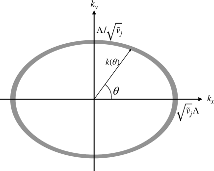
Figure 7: Ellipse momentum shell integration arsing from $v_{j}\neq\bar{v}$.

Based on this, it is straightforward to see (defining $\bm{R}=(\bm{r}_{1}+\bm{r}_{2})/2$)

$$\braket{S_{I}^{2}[\phi_{i}^{s}+h_{i}]}_{h}-\braket{S_{I}[\phi_{i}^{s}+h_{i}]}_{h}^{2}=\frac{u_{2}^{2}}{4}\int d^{2}\bm{R}d^{2}\bm{r} (1-2B_{13}dl)\{\cos(2\beta_{1}\phi_{1}^{s}(\bm{R}))\cos(2\beta_{3}\phi_{3}^{s}(\bm{R}))(-\beta_{1}^{2}F_{1}(\bm{r})-\beta_{3}^{2}F_{3}(\bm{r}))dl$$ (93)

$$+ \cos(2\beta_{1}\phi_{2}^{s}(\bm{R}))\cos(\beta_{3}\bm{r}\cdot\nabla_{R}\phi_{3}^{s}(\bm{R}))(\beta_{3}^{2}F_{3}(\bm{r})-\beta_{1}^{2}F_{1}(\bm{r}))dl$$

$$+ \cos(2\beta_{3}\phi_{3}^{s}(\bm{R}))\cos(\beta_{1}\bm{r}\cdot\nabla_{R}\phi_{1}^{s}(\bm{R}))(\beta_{1}^{2}F_{1}(\bm{r})-\beta_{3}^{2}F_{3}(\bm{r}))dl$$

$$+ \cos(\beta_{1}\bm{r}\cdot\nabla_{R}\phi_{1}^{s}(\bm{R}))\cos(\beta_{3}\bm{r}\cdot\nabla_{R}\phi_{3}^{s}(\bm{R}))(\beta_{1}^{2}F_{1}(\bm{r})+\beta_{3}^{2}F_{3}(\bm{r}))dl\}$$

$$+ u_{1}^{2}[...]+u_{3}^{2}[...]$$

$$+\frac{u_{2}u_{1}}{2}(1-(B_{13}+B_{23})dl)\int d^{2}\bm{R}d^{2}\bm{r}\{\cos[\beta_{1}\phi_{1}^{s}(\bm{R})+ \beta_{2}\phi_{3}^{s}(\bm{R})+\beta_{1}\frac{\bm{r}}{2}\cdot\nabla_{R}\phi_{1}^{s}(\bm{R})-\beta_{2}\frac{\bm{r}}{2}\cdot\nabla_{R}\phi_{2}^{s}(\bm{R})]\cos[2\beta_{3}\phi_{3}^{s}(\bm{R})](-\beta_{3}^{2})F_{3}(\bm{r})dl$$

$$+\cos[\beta_{1}\phi_{1}^{s}(\bm{R})+\beta_{2}\phi_{2}^{s}(\bm{R})+ \beta_{1}\frac{\bm{r}}{2}\cdot\nabla_{R}\phi_{1}^{s}(\bm{R})-\beta_{2}\frac{\bm{r}}{2}\cdot\nabla_{R}\phi_{2}^{s}(\bm{R})]\cos[\beta_{3}\bm{r}\cdot\nabla_{R}\phi_{3}^{s}(\bm{R})]\beta_{3}^{2}F_{3}(\bm{r})dl$$

$$+\cos[\beta_{1}\phi_{1}^{s}(\bm{R})-\beta_{2}\phi_{2}^{s}(\bm{R})+ \beta_{1}\frac{\bm{r}}{2}\cdot\nabla_{R}\phi_{1}^{s}(\bm{R})+\beta_{2}\frac{\bm{r}}{2}\cdot\nabla_{R}\phi_{2}^{s}(\bm{R})]\cos[2\beta_{3}\phi_{3}^{s}(\bm{R})](-\beta_{3}^{2})F_{3}(\bm{r})dl$$

$$+\cos[\beta_{1}\phi_{1}^{s}(\bm{R})-\beta_{2}\phi_{2}^{s}(\bm{R})+ \beta_{1}\frac{\bm{r}}{2}\cdot\nabla_{R}\phi_{1}^{s}(\bm{R})+\beta_{2}\frac{\bm{r}}{2}\cdot\nabla_{R}\phi_{2}^{s}(\bm{R})]\cos[\beta_{3}\bm{r}\cdot\nabla_{R}\phi_{3}^{s}(\bm{R})]\beta_{3}^{2}F_{3}(\bm{r})dl\}$$

$$+u_{2}u_{3}[...]+u_{1}u_{3}[...].$$

From the above expressions, we need to identify the ones which renormalize the gradient terms, i.e. $S_{0}[\phi_{i}]$. To this end, we assume we are close the the critical point, and all terms containing $\cos[2\beta_{j}\phi_{j}^{s}]$ are irrelevant. It’s easy to see only the squared terms ($u_{1}^{2}$, $u_{2}^{2}$ and $u_{3}^{2}$) contribute to the renormalization of $S_{0}$. In comparing to $S_{0}$ we note that $\nabla_{R}\phi_{j}=(\partial_{R_{x}}\phi_{j},\partial_{R_{y}}\phi_{j})$ is symmetric with respect to interchanging $R_{x}$ and $R_{y}$. However, we see from above that with $v_{j}\neq\bar{v}$ we have anisotropy. Thus, we will skew the coordinates of $\bm{r}$ to $\tilde{\bm{r}}$, such that

$$\bm{r}\cdot\nabla_{R}\phi_{j}=x\partial_{R_{x}}\phi_{j}+y\partial_{R_{y}}\phi_{j}=\frac{x}{\sqrt{\tilde{v}_{j}}}\sqrt{\tilde{v}_{j}}\partial_{R_{x}}\phi_{j}+y\sqrt{\tilde{v}_{j}}\frac{\partial_{R_{y}}\phi_{j}}{\sqrt{\tilde{v}_{j}}}:=\tilde{x}\sqrt{\tilde{v}_{j}}\partial_{R_{x}}\phi_{j}+\tilde{y}\frac{\partial_{R_{y}}\phi_{j}}{\sqrt{\tilde{v}_{j}}}$$ (94)

The measure is invariant under the change from $\bm{r}$ to $\tilde{\bm{r}}$ so we have, for instance,

$$\int d^{2}\bm{r}(\bm{r}\cdot\nabla_{R}\phi_{j})^{2}F_{j}(\bm{r})=\int d^{2}\tilde{\bm{r}}(\tilde{\bm{r}}\cdot\tilde{\nabla_{R}\phi_{j}})^{2}\tilde{F}_{j}(\tilde{\bm{r}})$$ (95)

where $\tilde{F}_{j}$ is given in Eq.(92). Introducing $\tilde{g}_{i}=g_{i}/\bar{v}$ such that $u_{i}=\tilde{g}_{i}/(\pi^{2}\alpha^{2})$, we have for the gradient terms after a straightforward manipulation

$$\frac{1}{2}\left[1+\left({\tilde{g}}_{2}^{2}(A_{1}\beta_{1}^{2}+A_{3}\beta_{3}^{2})+{\tilde{g}}_{3}^{2}(A_{1}\beta_{1}^{2}+A_{2}\beta_{2}^{2})\right)\frac{\beta_{1}^{2}}{8}dl\right]\int d^{2}\bm{r}\left(\tilde{v}_{1}(\partial_{x}\phi_{i})^{2}+\frac{1}{\tilde{v}_{1}}(\partial_{y}\phi_{i})^{2}\right)$$ (96)

$$+ \frac{1}{2}\left[1+\left({\tilde{g}}_{1}^{2}(A_{2}\beta_{2}^{2}+A_{3}\beta_{3}^{2})+{\tilde{g}}_{3}^{2}(A_{1}\beta_{1}^{2}+A_{2}\beta_{2}^{2})\right)\frac{\beta_{2}^{2}}{8}dl\right]\int d^{2}\bm{r}\left(\tilde{v}_{2}(\partial_{x}\phi_{i})^{2}+\frac{1}{\tilde{v}_{2}}(\partial_{y}\phi_{i})^{2}\right)$$

$$+ \frac{1}{2}\left[1+\left({\tilde{g}}_{2}^{2}(A_{1}\beta_{1}^{2}+A_{3}\beta_{3}^{2})+{\tilde{g}}_{1}^{2}(A_{2}\beta_{2}^{2}+A_{3}\beta_{3}^{2})\right)\frac{\beta_{3}^{2}}{8}dl\right]\int d^{2}\bm{r}\left(\tilde{v}_{3}(\partial_{x}\phi_{i})^{2}+\frac{1}{\tilde{v}_{3}}(\partial_{y}\phi_{i})^{2}\right)$$

Transforming this correction to the cosine terms (by rescaling the fields $\phi_{j}$), we obtain the following RG equations

$$\frac{d\beta_{1}^{2}}{dl} =-\left({\tilde{g}}_{2}^{2}(A_{1}\beta_{1}^{2}+A_{3}\beta_{3}^{2})+{\tilde{g}}_{3}^{2}(A_{1}\beta_{1}^{2}+A_{2}\beta_{2}^{2})\right)\frac{\beta_{1}^{4}}{8}$$ (97)

$$\frac{d\beta_{3}^{2}}{dl} =-\left({\tilde{g}}_{1}^{2}(A_{2}\beta_{2}^{2}+A_{3}\beta_{3}^{2})+{\tilde{g}}_{3}^{2}(A_{1}\beta_{1}^{2}+A_{2}\beta_{2}^{2})\right)\frac{\beta_{2}^{4}}{8}$$

$$\frac{d\beta_{3}^{2}}{dl} =-\left({\tilde{g}}_{2}^{2}(A_{1}\beta_{1}^{2}+A_{3}\beta_{3}^{2})+{\tilde{g}}_{1}^{2}(A_{2}\beta_{2}^{2}+A_{3}\beta_{3}^{2})\right)\frac{\beta_{3}^{4}}{8}$$

In terms of the Luttinger parameters,

$$\frac{dK_{1}}{dl} =-2\pi^{2}K_{1}^{2}\left[{\tilde{g}}_{2}^{2}(A_{1}K_{1}+A_{3}K_{3})+{\tilde{g}}_{3}^{2}(A_{1}K_{1}+A_{2}K_{2})\right],$$ (98)

$$\frac{dK_{2}}{dl} =-2\pi^{2}K_{2}^{2}\left[{\tilde{g}}_{1}^{2}(A_{2}K_{2}+A_{3}K_{3})+{\tilde{g}}_{3}^{2}(A_{1}K_{1}+A_{2}K_{2})\right],$$

$$\frac{dK_{3}}{dl} =-2\pi^{2}K_{3}^{2}\left[{\tilde{g}}_{2}^{2}(A_{1}K_{1}+A_{3}K_{3})+{\tilde{g}}_{1}^{2}(A_{2}K_{2}+A_{3}K_{3})\right].$$

Also note that the cross terms in Eq.(93), give rise to additional renormalization to the interactions in addition to Eq.(83).

$$\frac{d{\tilde{g}}_{1}}{dl} =\left[2-(K_{2}+K_{3})\right]{\tilde{g}}_{1}+4\pi A_{1}^{\prime}{\tilde{g}}_{2}{\tilde{g}}_{3}K_{1},$$ (99)

$$\frac{d{\tilde{g}}_{2}}{dl} =\left[2-(K_{1}+K_{3})\right]{\tilde{g}}_{2}+4\pi A_{2}^{\prime}{\tilde{g}}_{1}{\tilde{g}}_{3}K_{2},$$

$$\frac{d{\tilde{g}}_{3}}{dl} =\left[2-(K_{1}+K_{2})\right]{\tilde{g}}_{3}+4\pi A_{3}^{\prime}{\tilde{g}}_{2}{\tilde{g}}_{1}K_{3}.$$

where

$$A_{j}\approx\frac{\pi}{\pi^{4}\alpha^{4}}\int_{0}^{1/\Lambda}drr^{3}\tilde{F}_{j}(r),~{}~{}~{}A_{j}^{\prime}\approx\frac{2\pi}{\pi^{2}\alpha^{2}}\int_{0}^{1/\Lambda}drr\tilde{F}_{j}(r).$$ (100)

We can absorb the constants relating $\pi$ into the new definition of $A_{j}$ and $A_{j}^{\prime}$, so we end up with

$$\boxed{\begin{aligned} \frac{dK_{1}}{dl}&=-K_{1}^{2}\left[{\tilde{g}}_{2}^{2}(A_{1}K_{1}+A_{3}K_{3})+{\tilde{g}}_{3}^{2}(A_{1}K_{1}+A_{2}K_{2})\right],\\ \frac{dK_{2}}{dl}&=-K_{2}^{2}\left[{\tilde{g}}_{1}^{2}(A_{2}K_{2}+A_{3}K_{3})+{\tilde{g}}_{3}^{2}(A_{1}K_{1}+A_{2}K_{2})\right],\\ \frac{dK_{3}}{dl}&=-K_{3}^{2}\left[{\tilde{g}}_{2}^{2}(A_{1}K_{1}+A_{3}K_{3})+{\tilde{g}}_{1}^{2}(A_{2}K_{2}+A_{3}K_{3})\right],\\ \frac{d{\tilde{g}}_{1}}{dl}&=\left[2-(K_{2}+K_{3})\right]{\tilde{g}}_{1}+A_{1}^{\prime}{\tilde{g}}_{2}{\tilde{g}}_{3}K_{1},\\ \frac{d{\tilde{g}}_{2}}{dl}&=\left[2-(K_{1}+K_{3})\right]{\tilde{g}}_{2}+A_{2}^{\prime}{\tilde{g}}_{1}{\tilde{g}}_{3}K_{2},\\ \frac{d{\tilde{g}}_{3}}{dl}&=\left[2-(K_{1}+K_{2})\right]{\tilde{g}}_{3}+A_{3}^{\prime}{\tilde{g}}_{2}{\tilde{g}}_{1}K_{3}.\end{aligned}}$$ (101)

where the constants $A_{j}$ and $A_{j}^{\prime}$ are now given by

$$A_{j}\approx\frac{2\pi^{3}}{\pi^{4}\alpha^{4}}\int_{0}^{1/\Lambda}drr^{3}\tilde{F}_{j}(r),~{}~{}~{}A_{j}^{\prime}\approx\frac{8\pi^{2}}{\pi^{2}\alpha^{2}}\int_{0}^{1/\Lambda}drr\tilde{F}_{j}(r).$$ (102)

In zero temperature limit, we can use Eq.(92) and obtain (setting $\alpha\Lambda=1$)

$$A_{j}=\frac{1}{\pi^{2}(\alpha\Lambda)^{4}}\int_{0}^{1}dxx^{3}\tilde{F}_{j}(x)\approx 0.02+0.002\delta_{j},~{}~{}A_{j}^{\prime}=\frac{4}{\pi(\alpha\Lambda)^{2}}\int_{0}^{1}dxx\tilde{F}_{j}(x)\approx 0.56+0.035\delta_{j}.$$ (103)

where we remind that $\delta_{j}=\tilde{v}_{j}-1$.

In Fig.8 we show an example of the RG flows obtained by setting $\tilde{g}_{2}(0)=\tilde{g}_{3}(0)=0$ and $K_{2}(0)=K_{3}(0)$. In this case, $\tilde{g}_{2}$ and $\tilde{g}_{3}$ remain zero, $K_{1}$ does not flow, $K_{2}$ and $K_{3}$ remain identical which we denote by $K$. In the vicinity of $K\approx 1$ and $\tilde{g}_{1}\to 0$, this is the Kosterlitz-Thouless RG flow.

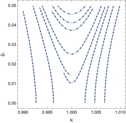
Figure 8: RG flows in the $\tilde{g}_{1}$-$K$ plane with the condition $K_{2}=K_{3}=K$ and $\tilde{g}_{2}=\tilde{g}_{3}=0$.

V V. Self-consistent Gaussian approximation for the massive phase

We now discuss when the three double-cosine terms in Eq.(73) are relevant, the gap can be determined self-consistently in a variational approach, also known as self-consistent Gaussian approximation. Let’s use the notations formulated in Eq.(44) and(45).

Deep inside the massive phase, we can approximate the action as some Gaussian form, expecting the soliton modes are excluded in the low energy limit. To this end, we write the variational Gaussian action as (for $i=1,2,3$)

$$S_{\text{var}}[\phi_{i}]=\frac{T}{2L}\sum_{n,q}\sum_{i,j}G^{-1}_{ij}(q,\omega_{n})\phi_{i}^{*}(q,\omega_{n})\phi_{j}(q,\omega_{n})$$ (104)

where

$$G^{-1}(\bm{q})=\begin{pmatrix}\frac{v_{1}}{\pi K_{1}}\left(\frac{\omega_{n}^{2}}{v_{1}^{2}}+q^{2}+\frac{\Delta_{1}^{2}}{v_{1}^{2}}\right)&\Delta_{12}&\Delta_{13}\\ \Delta_{21}&\frac{v_{2}}{\pi K_{2}}\left(\frac{\omega_{n}^{2}}{v_{2}^{2}}+q^{2}+\frac{\Delta_{2}^{2}}{v_{2}^{2}}\right)&\Delta_{23}\\ \Delta_{31}&\Delta_{32}&\frac{v_{3}}{\pi K_{3}}\left(\frac{\omega_{n}^{2}}{v_{3}^{2}}+q^{2}+\frac{\Delta_{3}^{2}}{v_{3}^{2}}\right)\end{pmatrix}$$ (105)

and $\Delta_{i}$ is the gap for the $i$-th sector. We will assume that $\Delta_{ij}=\Delta_{ji}$ so $G^{-1}$ is a symmetric matrix which can be diagonalize by an orthogonal matrix $U$:

$$\phi^{\dagger}G^{-1}\phi=\tilde{\phi}^{\dagger}G_{d}^{-1}\tilde{\phi}$$ (106)

where

$$\phi=U\tilde{\phi},~{}~{}G^{-1}=UG_{d}^{-1}U^{-1}$$ (107)

and $G_{d}$ is now a diagonal matrix.

The variational free energy to be minimized is,

$$F_{\text{var}}=-T\ln Z_{\text{var}}+T\braket{S-S_{\text{var}}}_{\text{var}}$$ (108)

where $Z_{\text{var}}$ is the partition function evaluated using $S_{\text{var}}$ and the original $S$ is given in Eqs.(44) and (45). The first term in Eq.(108) can be evaluated directly,

$$-T\ln Z_{\text{var}}=-T\text{Tr}\ln G(q,\omega_{n}).$$ (109)

Note in the second term, $\braket{S_{\text{var}}}_{\text{var}}$ does not contain dependence on the variational parameter, so it can be dropped. We are then left with evaluating $\braket{S}_{\text{var}}$, which involves in evaluating the average of the product of two cosine terms $g_{i}\cos(2\phi_{j})\cos(2\phi_{k})$ using the Gaussian distribution function. This requires one first identify the classical ground state of these cosine terms. In the case when there is no frustration, i.e. when $\operatorname{sgn}(g_{1}g_{2}g_{3})>0$, the classical ground state is easy to find. When all $g_{i}>0$, all $\phi_{i}$ should be around $\phi_{i}=0$. when $g_{i}>0$ and $g_{j},g_{k}<0$, we should have $\phi_{j,k}=0$ and $\phi_{i}=\pm\pi/2$. Since $\phi_{i}$ is around $\pm\pi/2$ we can shift $\phi_{i}$ by $\pm\pi/2$ such that $\cos 2\phi_{i}$ picks up a minus sign, which can be absorbed in $g_{j}$ and $g_{k}$. Therefore, in the case without frustration, we can use the absolute value of $g_{i,j,k}$ and then average all the cosine terms at $\phi_{i,j,k}$ around $0$.

$$\braket{S}_{\text{var}}=\sum_{i=1}^{3}\frac{v_{i}}{2\pi K_{i}}\sum_{n,q}\left(\frac{\omega_{n}^{2}}{v_{i}^{2}}+q^{2}\right)G_{i,i}(q,\omega_{n})$$ (110)

$$-\frac{1}{2\pi^{2}\alpha^{2}}\frac{L}{T}\left(|g_{1}|\braket{e^{i2(\phi_{2}+\phi_{3})}+e^{i2(\phi_{2}-\phi_{3})}}_{\text{var}}+|g_{2}|\braket{e^{i2(\phi_{3}+\phi_{1})}+e^{i2(\phi_{3}-\phi_{1})}}_{\text{var}}+|g_{3}|\braket{e^{i2(\phi_{1}+\phi_{2})}+e^{i2(\phi_{1}-\phi_{2})}}_{\text{var}}\right).$$

Here we average the $\cos(2\phi_{i})$ around $\phi_{i}=0$. Going to the $\tilde{\phi}$ basis, we have

$$\braket{e^{i2(\phi_{2}\pm\phi_{3})}}_{\text{var}}=\braket{e^{i2\sum_{j}(U_{2j}\pm U_{3j})\tilde{\phi}_{j}}}_{\text{var}}=e^{-\frac{2T}{L}\sum_{n,q}\sum_{j}(U_{2j}\pm U_{3j})^{2}G_{d,j}(q,\omega_{n})}.$$ (111)

Since $G_{d}$ is diagonal, and $U^{T}=U^{-1}$, we have

$$\braket{e^{i2(\phi_{2}\pm\phi_{3})}}_{\text{var}}=e^{-\frac{2T}{L}\sum_{n,q}(G_{22}+G_{33}\pm 2G_{23})}$$ (112)

and similarly for other two terms in Eq.(110). Therefore

$$\braket{S}_{\text{var}}=\sum_{i=1}^{3}\frac{v_{i}}{2\pi K_{i}}\sum_{n,q}\left(\frac{\omega_{n}^{2}}{v_{i}^{2}}+q^{2}\right)G_{i,i}(q,\omega_{n})-\frac{1}{\pi^{2}\alpha^{2}}\frac{L}{T}\times$$ (113)

$$\times\left(|g_{1}|e^{-\frac{2T}{L}\sum_{n,q}(G_{22}+G_{33})}\cosh[4\text{Tr}G_{23}]+|g_{2}|e^{-\frac{2T}{L}\sum_{n,q}(G_{11}+G_{33})}\cosh[4\text{Tr}G_{13}]+|g_{3}|e^{-\frac{2T}{L}\sum_{n,q}(G_{11}+G_{22})}\cosh[4\text{Tr}G_{12}]\right).$$

Here $\text{Tr}G_{ij}=\frac{T}{L}\sum_{q,n}G_{ij}(q,\omega_{n})$. To obtain $G$, we need to inverse the matrix $G^{-1}$. In the case when all $\Delta_{ij}$ are close to zero, we can approximately have

$$G(\bm{q})\approx\begin{pmatrix}\frac{\pi K_{1}}{v_{1}}\left(\frac{\omega_{n}^{2}}{v_{1}^{2}}+q^{2}+\frac{\Delta_{1}^{2}}{v_{1}^{2}}\right)^{-1}&-\frac{\pi^{2}K_{1}K_{2}}{v_{1}v_{2}}\frac{\Delta_{12}}{(\frac{\omega_{n}^{2}}{v_{1}^{2}}+q^{2}+\frac{\Delta_{1}^{2}}{v_{1}^{2}})(\frac{\omega_{n}^{2}}{v_{2}^{2}}+q^{2}+\frac{\Delta_{2}^{2}}{v_{2}^{2}})}&-\frac{\pi^{2}K_{1}K_{3}}{v_{1}v_{3}}\frac{\Delta_{13}}{(\frac{\omega_{n}^{2}}{v_{1}^{2}}+q^{2}+\frac{\Delta_{1}^{2}}{v_{1}^{2}})(\frac{\omega_{n}^{2}}{v_{3}^{2}}+q^{2}+\frac{\Delta_{3}^{2}}{v_{3}^{2}})}\\ -\frac{\pi^{2}K_{1}K_{2}}{v_{1}v_{2}}\frac{\Delta_{12}}{(\frac{\omega_{n}^{2}}{v_{1}^{2}}+q^{2}+\frac{\Delta_{1}^{2}}{v_{1}^{2}})(\frac{\omega_{n}^{2}}{v_{2}^{2}}+q^{2}+\frac{\Delta_{2}^{2}}{v_{2}^{2}})}&\frac{\pi K_{2}}{v_{2}}\left(\frac{\omega_{n}^{2}}{v_{2}^{2}}+q^{2}+\frac{\Delta_{2}^{2}}{v_{2}^{2}}\right)^{-1}&-\frac{\pi^{2}K_{2}K_{3}}{v_{2}v_{3}}\frac{\Delta_{23}}{(\frac{\omega_{n}^{2}}{v_{2}^{2}}+q^{2}+\frac{\Delta_{2}^{2}}{v_{2}^{2}})(\frac{\omega_{n}^{2}}{v_{3}^{2}}+q^{2}+\frac{\Delta_{3}^{2}}{v_{3}^{2}})}\\ -\frac{\pi^{2}K_{1}K_{3}}{v_{1}v_{3}}\frac{\Delta_{13}}{(\frac{\omega_{n}^{2}}{v_{1}^{2}}+q^{2}+\frac{\Delta_{1}^{2}}{v_{1}^{2}})(\frac{\omega_{n}^{2}}{v_{3}^{2}}+q^{2}+\frac{\Delta_{3}^{2}}{v_{3}^{2}})}&-\frac{\pi^{2}K_{2}K_{3}}{v_{2}v_{3}}\frac{\Delta_{23}}{(\frac{\omega_{n}^{2}}{v_{2}^{2}}+q^{2}+\frac{\Delta_{2}^{2}}{v_{2}^{2}})(\frac{\omega_{n}^{2}}{v_{3}^{2}}+q^{2}+\frac{\Delta_{3}^{2}}{v_{3}^{2}})}&\frac{\pi K_{3}}{v_{3}}\left(\frac{\omega_{n}^{2}}{v_{3}^{2}}+q^{2}+\frac{\Delta_{3}^{2}}{v_{3}^{2}}\right)^{-1}\end{pmatrix}$$ (114)

Setting the functional derivative $\delta F_{\text{var}}/\delta G_{ij}(q,\omega_{n})$ to zero, we arrive at the following coupled equations

$$G_{11}^{-1}(q,\omega_{n}) =\frac{v_{1}}{\pi K_{1}}\left(\frac{\omega_{n}^{2}}{v_{1}^{2}}+q^{2}\right)+\frac{4}{\pi^{2}\alpha^{2}}\left(|g_{2}|e^{-\frac{2T}{L}\sum_{n,q}[G_{11}+G_{33}]}\cos[4\text{Tr}G_{13}]+|g_{3}|e^{-\frac{2T}{L}\sum_{n,q}[G_{11}+G_{22}]}\cos[4\text{Tr}G_{12}]\right),$$ (115)

$$G_{22}^{-1}(q,\omega_{n}) =\frac{v_{2}}{\pi K_{2}}\left(\frac{\omega_{n}^{2}}{v_{2}^{2}}+q^{2}\right)+\frac{4}{\pi^{2}\alpha^{2}}\left(|g_{1}|e^{-\frac{2T}{L}\sum_{n,q}[G_{22}+G_{33}]}\cos[4\text{Tr}G_{23}]+|g_{3}|e^{-\frac{2T}{L}\sum_{n,q}[G_{11}+G_{22}]}\cos[4\text{Tr}G_{12}]\right),$$

$$G_{33}^{-1}(q,\omega_{n}) =\frac{v_{3}}{\pi K_{3}}\left(\frac{\omega_{n}^{2}}{v_{3}^{2}}+q^{2}\right)+\frac{4}{\pi^{2}\alpha^{2}}\left(|g_{2}|e^{-\frac{2T}{L}\sum_{n,q}[G_{11}+G_{33}]}\cos[4\text{Tr}G_{13}]+|g_{1}|e^{-\frac{2T}{L}\sum_{n,q}[G_{22}+G_{33}]}\cos[4\text{Tr}G_{23}]\right),$$

$$G_{12}^{-1}=\Delta_{12} =\frac{4}{\pi^{2}\alpha^{2}}|g_{3}|e^{-\frac{2T}{L}\sum_{n,q}[G_{11}+G_{22}]}\sinh[4\text{Tr}G_{12}],$$

$$G_{13}^{-1}=\Delta_{13} =\frac{4}{\pi^{2}\alpha^{2}}|g_{2}|e^{-\frac{2T}{L}\sum_{n,q}[G_{11}+G_{33}]}\sinh[4\text{Tr}G_{13}],$$

$$G_{23}^{-1}=\Delta_{23} =\frac{4}{\pi^{2}\alpha^{2}}|g_{1}|e^{-\frac{2T}{L}\sum_{n,q}[G_{22}+G_{33}]}\sinh[4\text{Tr}G_{23}].$$

From the above equations, it is apparent that $\Delta_{ij}=0$ is always satisfied. Below we adopt this solution, and the equations then become

$$G_{1}^{-1}(q,\omega_{n}) =\frac{v_{1}}{\pi K_{1}}\left(\frac{\omega_{n}^{2}}{v_{1}^{2}}+q^{2}\right)+\frac{4}{\pi^{2}\alpha^{2}}\left(|g_{2}|e^{-\frac{2T}{L}\sum_{n,q}[G_{1}(q,\omega_{n})+G_{3}(q,\omega_{n})]}+|g_{3}|e^{-\frac{2T}{L}\sum_{n,q}[G_{1}(q,\omega_{n})+G_{2}(q,\omega_{n})]}\right)$$ (116)

$$G_{2}^{-1}(q,\omega_{n}) =\frac{v_{2}}{\pi K_{2}}\left(\frac{\omega_{n}^{2}}{v_{2}^{2}}+q^{2}\right)+\frac{4}{\pi^{2}\alpha^{2}}\left(|g_{1}|e^{-\frac{2T}{L}\sum_{n,q}[G_{2}(q,\omega_{n})+G_{3}(q,\omega_{n})]}+|g_{3}|e^{-\frac{2T}{L}\sum_{n,q}[G_{1}(q,\omega_{n})+G_{2}(q,\omega_{n})]}\right)$$

$$G_{3}^{-1}(q,\omega_{n}) =\frac{v_{3}}{\pi K_{3}}\left(\frac{\omega_{n}^{2}}{v_{3}^{2}}+q^{2}\right)+\frac{4}{\pi^{2}\alpha^{2}}\left(|g_{2}|e^{-\frac{2T}{L}\sum_{n,q}[G_{1}(q,\omega_{n})+G_{3}(q,\omega_{n})]}+|g_{1}|e^{-\frac{2T}{L}\sum_{n,q}[G_{2}(q,\omega_{n})+G_{3}(q,\omega_{n})]}\right)$$

We can insert Eq.(114) to obtain equations for $\Delta_{i}$. We do this in the zero temperature limit, where

$$-\frac{2T}{L}\sum_{n,q}G_{i}(q,\omega_{n})=-2\pi K_{i}\int\frac{d^{2}\bm{q}}{(2\pi)^{2}}\frac{1}{\bm{q}^{2}+m_{i}^{2}}\approx-\frac{K_{i}}{2}\ln\left(1+\frac{\Lambda^{2}}{m_{i}^{2}}\right)$$ (117)

where $\Lambda$ is some UV cutoff for the momentum. Making use of this result, the equations for $\Delta_{i}$’s are

$$\delta_{1}^{2} =\frac{4K_{1}}{\pi v_{1}(\alpha\Lambda)^{2}}\left[|g_{2}|\left(\frac{\delta_{1}^{2}}{1+\delta_{1}^{2}}\right)^{\frac{K_{1}}{2}}\left(\frac{\delta_{3}^{2}}{1+\delta_{3}^{2}}\right)^{\frac{K_{3}}{2}}+|g_{3}|\left(\frac{\delta_{1}^{2}}{1+\delta_{1}^{2}}\right)^{\frac{K_{1}}{2}}\left(\frac{\delta_{2}^{2}}{1+\delta_{2}^{2}}\right)^{\frac{K_{2}}{2}}\right]$$ (118)

$$\delta_{2}^{2} =\frac{4K_{2}}{\pi v_{2}(\alpha\Lambda)^{2}}\left[|g_{1}|\left(\frac{\delta_{2}^{2}}{1+\delta_{2}^{2}}\right)^{\frac{K_{2}}{2}}\left(\frac{\delta_{3}^{2}}{1+\delta_{3}^{2}}\right)^{\frac{K_{3}}{2}}+|g_{3}|\left(\frac{\delta_{1}^{2}}{1+\delta_{1}^{2}}\right)^{\frac{K_{1}}{2}}\left(\frac{\delta_{2}^{2}}{1+\delta_{2}^{2}}\right)^{\frac{K_{2}}{2}}\right]$$

$$\delta_{3}^{2} =\frac{4K_{3}}{\pi v_{3}(\alpha\Lambda)^{2}}\left[|g_{2}|\left(\frac{\delta_{1}^{2}}{1+\delta_{1}^{2}}\right)^{\frac{K_{1}}{2}}\left(\frac{\delta_{3}^{2}}{1+\delta_{3}^{2}}\right)^{\frac{K_{3}}{2}}+|g_{1}|\left(\frac{\delta_{2}^{2}}{1+\delta_{2}^{2}}\right)^{\frac{K_{2}}{2}}\left(\frac{\delta_{3}^{2}}{1+\delta_{3}^{2}}\right)^{\frac{K_{3}}{2}}\right]$$

where we have used $\delta_{i}=\Delta_{i}/(v_{i}\Lambda)$. We usually deal with the case that $\delta_{i}\ll 1$, so the above equations become (setting $\alpha\Lambda=1$)

$$\delta_{1}^{2} =\frac{4K_{1}}{\pi v_{1}}|\delta_{1}|^{K_{1}}\left(|g_{2}||\delta_{3}|^{K_{3}}+|g_{3}||\delta_{2}|^{K_{2}}\right),$$ (119)

$$\delta_{2}^{2} =\frac{4K_{2}}{\pi v_{2}}|\delta_{2}|^{K_{2}}\left(|g_{1}||\delta_{3}|^{K_{3}}+|g_{3}||\delta_{1}|^{K_{1}}\right),$$

$$\delta_{3}^{2} =\frac{4K_{3}}{\pi v_{3}}|\delta_{3}|^{K_{3}}\left(|g_{2}||\delta_{1}|^{K_{1}}+|g_{1}||\delta_{2}|^{K_{2}}\right).$$

It is apparent from these equations that $\Delta_{i}=0$ is always a trivial solution.

The cases with frustration, i.e. when $\operatorname{sgn}(g_{1}g_{2}g_{3})<0$, are more involved, due to the possible presence of classically degenerate ground states. For instance, in the case when $g_{1}=g_{2}=g_{3}<0$, there exist several lines in the parameter space which correspond to the degenerate classical ground state. However, as we see from the RG analysis, this accidental symmetric case $g_{1}=g_{2}=g_{3}$ is not protected by any symmetry and is unstable, so we generally do not expect that they are all equal. Therefore, without loss of generality, we assume $|g_{1}|>|g_{2}|>|g_{3}|$. In this case, the classical ground state is unique. For instance, when all $g_{1,2,3}<0$, the classical ground state is $\phi_{1,2}=0$ and $\phi_{3}=\pm\pi/2$. After shifting $\phi_{3}$ by $\pm\pi/2$ we can still average every field around $0$. The derivation of the gap equations is parallel to outlined above, with the only difference being the replacement of $|g_{3}|$ with $-|g_{3}|$. Therefore, we obtain the gap equations for the case with frustration

$$\delta_{1}^{2} =\frac{4K_{1}}{\pi v_{1}}|\delta_{1}|^{K_{1}}\left(|g_{2}||\delta_{3}|^{K_{3}}-|g_{3}||\delta_{2}|^{K_{2}}\right),$$ (120)

$$\delta_{2}^{2} =\frac{4K_{2}}{\pi v_{2}}|\delta_{2}|^{K_{2}}\left(|g_{1}||\delta_{3}|^{K_{3}}-|g_{3}||\delta_{1}|^{K_{1}}\right),$$

$$\delta_{3}^{2} =\frac{4K_{3}}{\pi v_{3}}|\delta_{3}|^{K_{3}}\left(|g_{2}||\delta_{1}|^{K_{1}}+|g_{1}||\delta_{2}|^{K_{2}}\right).$$

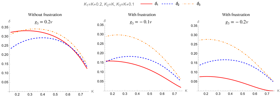
Figure 9: Solution of the gap equations with and without frustration. Here we choose $v_{1,2,3}=v$ and $g_{1}=0.3v$, $g_{2}=0.25v$. The Luttinger parameters are shown in the figure. In the case without frustration (left panel and solved from Eq.(119)), $\Delta_{1,2,3}$ are comparable to each other. In the case with frustration (middle and right panels, solved from Eq.(120)), all gaps get suppressed compared to the case without frustration. In particular, $\Delta_{1}$ gets suppressed the most and when $|g_{3}|$ gets larger, it becomes the smallest compared to $\Delta_{2}$ and $\Delta_{3}$.

In Fig.(9), we shown the comparison between the solutions of Eq.(119) and Eq.(120). We choose the parameters $v_{1,2,3}=v$, $g_{1}=0.3v$, $g_{2}=0.25v$, $K_{1}-0.2=K_{3}-0.1=K_{2}=K$ such that in the case without frustration all induced gaps are comparable. We clearly see from the middle and right panels of Fig.(9) that in the presence of frustration, all gaps get suppressed compared to the case without frustration. $\Delta_{1}$ gets suppressed the most and when $|g_{3}|$ gets as large as $0.2v$, it becomes much smaller than the other two and therefore a gap hierarchy develops.

VI VI. Transport property

We first show if only the CDW order is considered in the inter-wire coupling, there is no transverse current. To see this, we note the inter-wire coupling Hamiltonian for CDW order is

$$H_{c} =J\sum_{\braket{ij}}\int dxO_{\text{CDW}}^{\dagger}(i,x)O_{\text{CDW}}(j,x)+\text{h.c.}$$ (121)

$$=J\sum_{\braket{ij},\lambda\lambda^{\prime}}\int dx\psi^{\dagger}_{i,-,\lambda}(x)\psi_{i,+,\lambda}(x)\psi^{\dagger}_{j,+,\lambda^{\prime}}(x)\psi_{j,-,\lambda^{\prime}}(x)+(i\leftrightarrow j).$$

which is the most relevant one when the system is in the massive phase with gaps in all $\phi_{2},\phi_{3},\phi_{4}$ sectors and in the presence of strong repulsion. From this Hamiltonian, one can calculate the current density operator from the continuity equation $\partial_{y}j_{y}=i[\rho(i,x),H_{c}]=0$ and find the current vanishes. Note the vanishing is local, i.e. it’s not because two current operators on $i$ and $j$ cancel each other, but rather the current on each wire vanishes. Therefore, we see that by only turning on the CDW coupling is not enough for obtaining a finite cross-wire conductivity, we must have other couplings.

The most trivial one, will be the single particle tunneling (keeping only the nearest neighbor),

$$H_{t}=t_{\bot}\sum_{i,rr^{\prime},\lambda}\int dx\psi_{r,\lambda}^{\dagger}(i,x)\psi_{r^{\prime},\lambda}(i+1,x)+\text{h.c.}$$ (122)

The tunneling charge current due to the presence of this Hamiltonian is given by the continuity equation, and we obtain

$$j_{y}(i,x) =ict_{\bot}\sum_{r,\lambda}\left(\psi^{\dagger}_{r,\lambda}(i,x)\psi_{r,\lambda}(i+1,x)-\psi^{\dagger}_{r,\lambda}(i+1,x)\psi_{r,\lambda}(i,x)\right),$$ (123)

$$j_{y}(q_{y},x) =-2ct_{\bot}\sum_{r,\lambda}\int_{-\pi}^{\pi}dk_{y}\psi^{\dagger}_{r,\lambda}(k_{y}-\frac{q_{y}}{2},x)\psi_{r,\lambda}(k_{y}+\frac{q_{y}}{2},x)\sin k_{y}e^{i\frac{q_{y}}{2}},$$

where $c$ is the spacing between adjacent wires, and since $j_{y}(i,x)$ is Hermitian, $j_{y}(q_{y},x)^{\dagger}=j_{y}(-q_{y},x).$ Below, we will evaluate the current-current correlation in the Hamiltonian without $H_{t}$, similar to the approach in Ref.[110]. However, we will keep $H_{c}$ to the first order as in a perturbation theory. According to Kubo formula, the real part of conductivity is given by

$$\text{Re}\sigma_{\bot}(\omega)=-\frac{e^{2}}{\omega}\text{Im}\left[\lim_{q_{y}\to 0}\int dx\Pi_{\bot}^{R}(q_{y},x,\omega)\right]$$ (124)

where $\Pi_{\bot}^{R}(q_{y},x,\omega)$ is the Fourier transform of the retarded current-current correlation function, which can be obtained from

$$\Pi_{\bot}(q_{y},x,i\omega_{n})=\braket{j_{y}(q_{y},x,i\omega_{n})j_{y}(-q_{y},0,-i\omega_{n})}$$ (125)

by analytic continuation. Here we have assumed translation symmetry. To the first order in $H_{c}$, we have

$$\lim_{q_{y}\to 0}\int dx\Pi_{\bot}(q_{y},x,i\omega_{n})=\frac{1}{\beta}\sum_{ik_{n}}\sum_{r,\lambda}\int\frac{dk_{x}dk_{y}}{(2\pi)^{2}}4c^{2}t_{\bot}^{2}\sin^{2}k_{y}G_{r,\lambda}(k_{x},ik_{n})G_{r,\lambda}(k_{x},ik_{n}+i\omega_{n})$$ (126)

$$+ \frac{J}{\beta^{2}}\sum_{ik_{n},ip_{n}}\sum_{r,\lambda}\int\frac{d^{2}\bm{k}d^{2}\bm{p}}{(2\pi)^{4}}4c^{2}t_{\bot}^{2}\sin^{2}k_{y}\sin^{2}p_{y}G_{r,\lambda}(k_{x},ik_{n})G_{r,\lambda}(k_{x},ik_{n}+i\omega_{n})G_{-r,\lambda}(p_{x},ip_{n})G_{-r,\lambda}(p_{x},ip_{n}+i\omega_{n}).$$

Here we used the fact that all the Green’s functions are evaluated in the decoupled Hamiltonian, so these are essentially 1D Hamiltonians and do not depend on $k_{y}$ or the wire index. Note in the second line of Eq.(126) the difference in the $r$-index between these Green’s functions are due to the nature of the CDW interaction $H_{c}$. Upon expressing the Green’s functions using their spectral representations

$$G(k_{x},ik_{n})=\frac{1}{2\pi}\int d\varepsilon\frac{A(k_{x},\varepsilon)}{ik_{n}-\varepsilon},~{}~{}A(k_{x},\varepsilon)=-2\text{Im}G^{R}(k_{x},\varepsilon)$$ (127)

and analytically continuing on the real frequency axis by changing $i\omega_{n}$ to $\omega+i0^{+}$, we obtain (after summing over $ik_{n}$)

$$\text{Re}\sigma_{\bot}(\omega)=\frac{e^{2}ct_{\bot}^{2}}{2\pi}\sum_{r,\lambda}\int dx\int d\varepsilon\frac{n_{F}(\varepsilon)-n_{F}(\varepsilon+\omega)}{\omega}A_{r,\lambda}(x,\varepsilon)A_{r,\lambda}(-x,\varepsilon+\omega)$$ (128)

$$+\frac{e^{2}Jt_{\bot}^{2}}{8\pi^{3}}\sum_{r,\lambda}\int dxdx^{\prime}P\int d\epsilon d\epsilon^{\prime}\frac{n_{F}(\epsilon)-n_{F}(\epsilon^{\prime})}{\omega+\epsilon-\epsilon^{\prime}}A_{r,\lambda}(x,\epsilon)A_{r,\lambda}(-x,\epsilon^{\prime})\int d\varepsilon\frac{n_{F}(\varepsilon)-n_{F}(\varepsilon+\omega)}{\omega}A_{-r,\lambda}(x^{\prime},\varepsilon)A_{-r,\lambda}(-x^{\prime},\varepsilon+\omega),$$

where in the second line we use $P\int$ to denote the principle value integral. To proceed with obtaining the temperature , we need the spectral function for the decoupled 1D system. But here we can estimate the magnitude of $\sigma_{\bot}$ from the its prefactors (after restoring $\hbar$ everywhere),

$$\sigma_{\bot}(T)=\frac{e^{2}}{h}4(ack_{F}^{2})\left(\frac{t_{\bot}}{E_{F}}\right)^{2}F\left(\frac{T}{E_{F}}\right)\approx 18\frac{e^{2}}{h}\left(\frac{t_{\bot}}{E_{F}}\right)^{2}F\left(\frac{T}{E_{F}}\right)~{}~{}\text{for}~{}~{}k_{F}\approx\frac{\pi}{2a}$$ (129)

where $F$ is some dimensionless function that comes from the integral involving the spectral functions.

VI.1 A. Single-particle tunneling in the gapless case

We begin by discussing the conductivity due to the single particle tunneling process in the gapless case, i.e. all the four $\phi_{j}$ fields are gapless. As shown above, this requires the calculation of the single particle spectral function. By definition, the retarded single particle Green’s function is given by

$$G^{R}_{r,\lambda}(x,t)=-i\Theta(t)\braket{\{\psi_{r,\lambda}(x,t),\psi^{\dagger}_{r,\lambda}(0,0)\}}=-i\Theta(t)(G_{r,\lambda}(x,t)+G_{r,\lambda}(-x,-t))$$ (130)

where

$$G_{r,\lambda}(x,t)=\lim_{\alpha\to 0}\frac{e^{irk_{F}x}}{2\pi\alpha}\braket{e^{i\theta_{\lambda}(x,t)-ir\phi_{\lambda}(x,t)}e^{-i\theta_{\lambda}(0,0)+ir\phi_{\lambda}(0,0)}}$$ (131)

according to Eq.(25). Without loss of generality, we take $r=+$ and $\lambda=\uparrow u$. Using Eq.(27) we have

$$G_{r,\lambda}(x,t)=\lim_{\alpha\to 0}\frac{e^{irk_{F}x}}{2\pi\alpha}\prod_{j=0}^{3}\braket{e^{\frac{i}{2}[\theta_{j}(x,t)-\phi_{j}(x,t)]}e^{-\frac{i}{2}[\theta_{j}(0,0)-\phi_{j}(0,0)]}}_{j}$$ (132)

For Gaussian models we have $\braket{e^{iA}e^{-iB}}=\exp\left(-\frac{1}{2}\braket{A^{2}}-\frac{1}{2}\braket{B^{2}}+\braket{AB}\right)$, thus

$$\braket{e^{\frac{i}{2}[\theta_{j}(x,t)-\phi_{j}(x,t)]}e^{-\frac{i}{2}[\theta_{j}(0,0)-\phi_{j}(0,0)]}}_{j}=\exp\left[\frac{1}{4}\braket{\left(\theta_{j}(x,t)-\phi_{j}(x,t)\right)\left(\theta_{j}(0,0)-\phi_{j}(0,0)\right)}_{j}-\frac{1}{4}\braket{(\theta_{j}-\phi_{j})^{2}}_{j}\right].$$ (133)

Using Eq.(46), (47) and (48), it is easy to see

$$\braket{e^{\frac{i}{2}[\theta_{j}(x,t)-\phi_{j}(x,t)]}e^{-\frac{i}{2}[\theta_{j}(0,0)-\phi_{j}(0,0)]}}_{j}=\left(\frac{a}{a+i(v_{j}t-x)}\right)^{1/4}\left(\frac{a^{2}}{x^{2}+(iv_{j}t+a)^{2}}\right)^{\frac{K_{j}+\frac{1}{K_{j}}-2}{16}}.$$ (134)

As a result, we have,

$$G_{+,\uparrow A}(x,t)=\frac{e^{ik_{F}x}}{2\pi}\prod_{j=0}^{3}\left(\frac{1}{a+i(v_{j}t-x)}\right)^{1/4}\left(\frac{a^{2}}{x^{2}+(iv_{j}t+a)^{2}}\right)^{\gamma_{j}/2},~{}~{}~{}\gamma_{j}=\frac{K_{j}+\frac{1}{K_{j}}-2}{8}$$ (135)

In fact, this form does not depend on $\lambda$. For $r=-$, the only changes is to replace $x$ with $-x$ in the above expression.

For comparison, we note in the conventional two-component case, we have

$$G(x,t)\sim\prod_{j=c,s}\left(\frac{1}{a+i(v_{j}t-x)}\right)^{1/2}\left(\frac{a^{2}}{x^{2}+(iv_{j}t+a)^{2}}\right)^{\gamma_{j}/2},~{}~{}~{}\gamma_{j}=\frac{K_{j}+\frac{1}{K_{j}}-2}{4}.$$ (136)

Using this result, and if we neglect the correction due to the CDW order coupling, we have

$$\text{Re}\sigma_{\bot}(\omega\to 0,T) \sim\int dx\int d\varepsilon\frac{1}{4T}\text{sech}^{2}\left(\frac{\varepsilon}{2T}\right)A(x,\varepsilon)A(-x,\varepsilon+\omega)$$ (137)

$$\sim\int dx\int d\varepsilon\frac{1}{4T}\text{sech}^{2}\left(\frac{\varepsilon}{2T}\right)F(x,\varepsilon)$$

where $F(x,\varepsilon)$ obeys

$$F\left(ax,\frac{\varepsilon}{a}\right)=\frac{1}{a^{2\gamma}}F(x,\varepsilon),~{}~{}~{}\gamma=\sum_{j}\gamma_{j}.$$ (138)

The spectral function $A(x,\varepsilon)$ has the following properties:

$$A(x=0,\varepsilon)=N(\varepsilon)\sim|\varepsilon|^{\gamma},~{}~{}~{}A(x\gg 1/\varepsilon,\varepsilon)\sim\frac{\cos{\varepsilon x}}{x^{\gamma}},$$ (139)

so the function $F(x,\varepsilon)$ behaves like

$$F(x,\varepsilon) \sim\varepsilon^{2\gamma}~{}\text{for}~{}x\ll 1/\varepsilon,$$ (140)

$$\sim\frac{1}{x^{2\gamma}}~{}\text{for}~{}x\gg 1/\varepsilon.$$

Therefore

$$\text{Re}\sigma_{\bot}(\omega\to 0,T)\sim\int d\varepsilon\frac{1}{4T}\text{sech}^{2}\left(\frac{\varepsilon}{2T}\right)\left(\int_{0}^{1/\varepsilon}dx\varepsilon^{2\gamma}+\int_{1/\varepsilon}^{+\infty}dx\frac{\cos{2\varepsilon x}}{x^{2\gamma}}\right)\sim T^{2\gamma-1}.$$ (141)

In the main text, we introduce the scaling dimension of the single particle hopping $\alpha_{e}$, which is related to $\gamma$ simply by $\gamma=\alpha_{e}-1$.

VI.2 B. Single-particle tunneling in the gapped case

When there is a gap opening in either one or more of the $\phi_{j}$ fields, the total single particle density of states has a gap structure. This is because the total real pace Green’s function is a product of the four component, as shown in Eq.(135). Consequently, the spectral function (and hence the density of states), which is the Fourier transform of Eq.(135), is a convolution of different components. It is this convolution that leads to a gap in the total spectral function. For two component 1DEG this was demonstrated in Ref.[109] If there is a gap in the total density of states, the conductivity becomes zero when $T$ is below the gap energy scale. However, when $T$ is well above the energy scale set by the gap, Eq.(141) still applies.

VI.3 C. Josephson tunneling in the gapped case

Unlike the single particle tunneling, the pair or quadruple hopping process does not depend on the single particle density of states, and can contribute to the cross wire conductivity even in the gapped phase and when $T$ not well above the gap energy scale. Below we discuss this Josephson tunneling due to charge-2e and charge-4e orders.

VI.3.1 charge-2e superconductivity

We take spin-triplet pseudospin-triplet pairing order parameter in Eq.(68) as an example. Assuming we are in the partially gapped phase when $\phi_{2,3}$ are gapped. The tunneling is governed by the Hamiltonian

$$H_{J} =J_{s}\sum_{\braket{y,y^{\prime}}}\int dxO_{T_{1},S}^{\dagger}(x,y)O_{T_{1},S}(x,y^{\prime})+\text{h.c.}$$ (142)

$$=\tilde{J}_{s}\sum_{\braket{y,y^{\prime}}}\int dx\cos\left[\theta_{0}(x,y)+\theta_{1}(x,y)-\theta_{0}(x,y^{\prime})-\theta_{1}(x,y^{\prime})\right],$$

where $\tilde{J}_{s}=J_{s}\delta_{2}^{K_{2}/2}\delta_{3}^{K_{3}/2}$ and $J_{s}\sim t_{\bot}^{2}/E_{F}$. On the other hand, the local charge density operator is given by $\rho_{0}(x,y)=\frac{1}{\pi}\partial_{x}\phi_{0}(x,y)$. Then according to the continuity equation, the transverse current density is found to be

$$j_{y}(x)=\tilde{J}_{s}c\sin[\theta_{0}(x,y+1)+\theta_{1}(x,y+1)-\theta_{0}(x,y)-\theta_{1}(x,y)]$$ (143)

which is the Josephson current. To evaluate the current-current correlation in the decoupled 1D system, we note that only the correlation involving two current operators with the same $y$ survives. Thus we have

$$\Pi_{\bot}(x,y,\tau) =\tilde{J}_{s}^{2}c^{2}\braket{\sin[\theta_{0}(x,y+1)+\theta_{1}(x,y+1)-\theta_{0}(x,y)-\theta_{1}(x,y)]\sin[\theta_{0}(0,0+1)+\theta_{1}(0,0+1)-\theta_{0}(0,0)-\theta_{1}(0,0)]}$$ (144)

$$=\frac{\tilde{J}_{s}^{2}c^{2}}{2}\left(\frac{a^{2}}{x^{2}+v_{0}^{2}\tau^{2}+a^{2}}\right)^{\frac{1}{2K_{0}}+\frac{1}{2K_{1}}}\delta_{y,0}.$$

Therefore

$$\Pi_{\bot}(\bm{q}\to 0,\omega)=\int dxdte^{i\omega t}\sum_{y}\Pi_{\bot}(x,y,t)\sim\tilde{J}_{s}^{2}c^{2}\omega^{1/K_{0}+1/K_{1}-2}$$ (145)

and

$$\text{Re}\sigma(\omega)\sim\tilde{J}_{s}^{2}c^{2}\omega^{1/K_{0}+1/K_{1}-3}\to\text{Re}\sigma(T)\sim\tilde{J}_{s}^{2}c^{2}T^{1/K_{0}+1/K_{1}-3}.$$ (146)

VI.3.2 charge-4e superconductivity

Like the charge-2e superconductivity case, the tunneling current is determined by the coupling Hamiltonian,

$$H_{J} =\tilde{J}_{s}\sum_{\braket{y,y^{\prime}}}\int dx\cos\left[2\theta_{0}(x,y)-2\theta_{0}(x,y^{\prime})\right].$$ (147)

The resulting current operator is

$$j_{y}(x)=\tilde{J}_{s}c\sin[2\theta_{0}(x,y+1)-2\theta_{0}(x,y)].$$ (148)

The calculation of conductivity is exactly the same as the 2e-SC case, with the modification of $\theta_{0}\to 2\theta_{0}$ and hence $1/K_{0}\to 4/K_{0}$, and the final result is

$$\text{Re}\sigma(T)\sim\tilde{J}_{s}^{2}c^{2}T^{4/K_{0}-3}$$ (149)

References

Emery [1979]V. Emery, Theory of the
one-dimensional electron gas, in Highly conducting one-dimensional solids (Springer, 1979) pp. 247–303.
Lorenz et al. [2002]T. Lorenz, M. Hofmann,
M. Grüninger, A. Freimuth, G. S. Uhrig, M. Dumm, and M. Dressel, Evidence for spin–charge separation in quasi-one-dimensional
organic conductors, Nature 418, 614 (2002).
Lebed [2008]A. G. Lebed, The physics of organic
superconductors and conductors, Vol. 110 (Springer, 2008).
Bao et al. [2015]J.-K. Bao, J.-Y. Liu,
C.-W. Ma, Z.-H. Meng, Z.-T. Tang, Y.-L. Sun, H.-F. Zhai, H. Jiang, H. Bai, C.-M. Feng, Z.-A. Xu, and G.-H. Cao, Superconductivity in
quasi-one-dimensional
with significant electron correlations, Phys. Rev. X 5, 011013 (2015).
Zhi et al. [2015]H. Z. Zhi, T. Imai, F. L. Ning, J.-K. Bao, and G.-H. Cao, Nmr investigation of the quasi-one-dimensional superconductor
, Phys. Rev. Lett. 114, 147004 (2015).
Tang et al. [2015a]Z.-T. Tang, J.-K. Bao,
Y. Liu, Y.-L. Sun, A. Ablimit, H.-F. Zhai, H. Jiang, C.-M. Feng,
Z.-A. Xu, and G.-H. Cao, Unconventional superconductivity in quasi-one-dimensional
, Phys. Rev. B 91, 020506 (2015a).
Tang et al. [2015b]Z.-T. Tang, J.-K. Bao,
Z. Wang, H. Bai, H. Jiang, Y. Liu, H.-F. Zhai, C.-M. Feng, Z.-A. Xu, and G.-H. Cao, Superconductivity in quasi-one-dimensional
Cs2Cr3As3 with large interchain distance, Science China Materials 58, 16 (2015b).
Tranquada et al. [1995]J. M. Tranquada, B. J. Sternlieb, J. D. Axe,
Y. Nakamura, and S. Uchida, Evidence for stripe correlations of spins and
holes in copper oxide superconductors, Nature 375, 561
(1995).
Orgad et al. [2001]D. Orgad, S. A. Kivelson,
E. W. Carlson, V. J. Emery, X. J. Zhou, and Z. X. Shen, Evidence of electron fractionalization from photoemission spectra in
the high temperature superconductors, Phys. Rev. Lett. 86, 4362 (2001).
Carlson et al. [2000]E. W. Carlson, D. Orgad,
S. A. Kivelson, and V. J. Emery, Dimensional crossover in quasi-one-dimensional and
high- superconductors, Phys. Rev. B 62, 3422 (2000).
Emery et al. [1997]V. J. Emery, S. A. Kivelson, and O. Zachar, Spin-gap proximity effect
mechanism of high-temperature superconductivity, Phys. Rev. B 56, 6120 (1997).
Ando et al. [2002]Y. Ando, K. Segawa,
S. Komiya, and A. N. Lavrov, Electrical resistivity anisotropy from self-organized one
dimensionality in high-temperature superconductors, Phys. Rev. Lett. 88, 137005 (2002).
Kivelson et al. [1998]S. A. Kivelson, E. Fradkin, and V. J. Emery, Electronic liquid-crystal phases of a
doped mott insulator, Nature 393, 550 (1998).
Emery et al. [2000]V. J. Emery, E. Fradkin,
S. A. Kivelson, and T. C. Lubensky, Quantum theory of the smectic metal
state in stripe phases, Phys. Rev. Lett. 85, 2160 (2000).
Mukhopadhyay et al. [2001a]R. Mukhopadhyay, C. L. Kane, and T. C. Lubensky, Sliding luttinger liquid
phases, Phys. Rev. B 64, 045120 (2001a).
Vishwanath and Carpentier [2001]A. Vishwanath and D. Carpentier, Two-dimensional
anisotropic non-fermi-liquid phase of coupled luttinger liquids, Phys. Rev. Lett. 86, 676 (2001).
Mukhopadhyay et al. [2001b]R. Mukhopadhyay, C. L. Kane, and T. C. Lubensky, Crossed sliding
luttinger liquid phase, Phys. Rev. B 63, 081103 (2001b).
Santos et al. [2015]R. A. Santos, C.-W. Huang,
Y. Gefen, and D. B. Gutman, Fractional topological insulators: From sliding luttinger
liquids to chern-simons theory, Phys. Rev. B 91, 205141 (2015).
Sur and Yang [2017]S. Sur and K. Yang, Coulomb interaction driven
instabilities of sliding luttinger liquids, Phys. Rev. B 96, 075131 (2017).
Chudnovskiy et al. [2017]A. L. Chudnovskiy, V. Kagalovsky, and I. V. Yurkevich, Metal-insulator
transition in a sliding luttinger liquid with line defects, Phys. Rev. B 96, 165111 (2017).
Sindzingre et al. [2002]P. Sindzingre, J.-B. Fouet, and C. Lhuillier, One-dimensional
behavior and sliding luttinger liquid phase in a frustrated
spin- crossed chain model: Contribution of exact
diagonalizations, Phys. Rev. B 66, 174424 (2002).
Plamadeala et al. [2014]E. Plamadeala, M. Mulligan, and C. Nayak, Perfect metal phases of
one-dimensional and anisotropic higher-dimensional systems, Phys. Rev. B 90, 241101 (2014).
Du et al. [2023]X. Du, L. Kang, Y. Y. Lv, J. S. Zhou, X. Gu, R. Z. Xu, Q. Q. Zhang, Z. X. Yin, W. X. Zhao,
Y. D. Li, S. M. He, D. Pei, Y. B. Chen, M. X. Wang, Z. K. Liu, Y. L. Chen, and L. X. Yang, Crossed luttinger liquid hidden in a
quasi-two-dimensional material, Nature Physics 19, 40 (2023).
Hu et al. [2023]Y. Hu, Y. Xu, and B. Lian, Twisted coupled wire model for moiré sliding luttinger
liquid (2023), arXiv:2310.04070 [cond-mat.str-el]
.
Cohn et al. [2023]J. L. Cohn, C. A. M. dos
Santos, and J. J. Neumeier, Superconductivity at
carrier density
in
quasi-one-dimensional , Phys. Rev. B 108, L100512 (2023).
Lu et al. [2019]J. Lu, X. Xu, M. Greenblatt, R. Jin, P. Tinnemans, S. Licciardello, M. R. van Delft, J. Buhot, P. Chudzinski, and N. E. Hussey, Emergence of a real-space symmetry
axis in the magnetoresistance of the one-dimensional conductor
Li0.9Mo6O, Science Advances 5, eaar8027 (2019).
Dudy et al. [2012]L. Dudy, J. D. Denlinger,
J. W. Allen, F. Wang, J. He, D. Hitchcock, A. Sekiyama, and S. Suga, Photoemission spectroscopy and the unusually robust one-dimensional physics
of lithium purple bronze, Journal of Physics: Condensed Matter 25, 014007 (2012).
Wang et al. [2022]P. Wang, G. Yu, Y. H. Kwan, Y. Jia, S. Lei, S. Klemenz, F. A. Cevallos, R. Singha,
T. Devakul, K. Watanabe, T. Taniguchi, S. L. Sondhi, R. J. Cava, L. M. Schoop, S. A. Parameswaran, and S. Wu, One-dimensional luttinger liquids in a two-dimensional moiré
lattice, Nature 605, 57 (2022).
Yu et al. [2023]G. Yu, P. Wang, A. J. Uzan, Y. Jia, M. Onyszczak, R. Singha, X. Gui, T. Song, Y. Tang, K. Watanabe, T. Taniguchi, R. J. Cava, L. M. Schoop, and S. Wu, Evidence for two dimensional anisotropic luttinger liquids at millikelvin
temperatures (2023), arXiv:2307.15881 [cond-mat.mes-hall]
.
Tang et al. [2020]Y. Tang, L. Li, T. Li, Y. Xu, S. Liu, K. Barmak, K. Watanabe,
T. Taniguchi, A. H. MacDonald, J. Shan, and K. F. Mak, Simulation of hubbard model physics in wse2/ws2 moiré
superlattices, Nature 579, 353 (2020).
Regan et al. [2020]E. C. Regan, D. Wang,
C. Jin, M. I. Bakti Utama, B. Gao, X. Wei, S. Zhao, W. Zhao, Z. Zhang, K. Yumigeta, M. Blei, J. D. Carlström, K. Watanabe, T. Taniguchi, S. Tongay, M. Crommie, A. Zettl, and F. Wang, Mott and
generalized wigner crystal states in wse2/ws2 moiré superlattices, Nature 579, 359 (2020).
Xu et al. [2020]Y. Xu, S. Liu, D. A. Rhodes, K. Watanabe, T. Taniguchi, J. Hone, V. Elser, K. F. Mak, and J. Shan, Correlated insulating states
at fractional fillings of moiré superlattices, Nature 587, 214 (2020).
Jin et al. [2021]C. Jin, Z. Tao, T. Li, Y. Xu, Y. Tang, J. Zhu, S. Liu, K. Watanabe, T. Taniguchi, J. C. Hone, L. Fu, J. Shan, and K. F. Mak, Stripe phases in
wse2/ws2 moiré superlattices, Nature Materials 20, 940 (2021).
Huang et al. [2021]X. Huang, T. Wang,
S. Miao, C. Wang, Z. Li, Z. Lian, T. Taniguchi,
K. Watanabe, S. Okamoto, D. Xiao, S.-F. Shi, and Y.-T. Cui, Correlated
insulating states at fractional fillings of the ws2/wse2 moiré lattice, Nature Physics 17, 715 (2021).
Li et al. [2021a]T. Li, S. Jiang, L. Li, Y. Zhang, K. Kang, J. Zhu, K. Watanabe,
T. Taniguchi, D. Chowdhury, L. Fu, J. Shan, and K. F. Mak, Continuous mott
transition in semiconductor moiré superlattices, Nature 597, 350 (2021a).
Wang et al. [2020]L. Wang, E.-M. Shih,
A. Ghiotto, L. Xian, D. A. Rhodes, C. Tan, M. Claassen, D. M. Kennes, Y. Bai, B. Kim, K. Watanabe, T. Taniguchi, X. Zhu, J. Hone, A. Rubio, A. N. Pasupathy, and C. R. Dean, Correlated electronic phases
in twisted bilayer transition metal dichalcogenides, Nature Materials 19, 861 (2020).
Ghiotto et al. [2021]A. Ghiotto, E.-M. Shih,
G. S. S. G. Pereira,
D. A. Rhodes, B. Kim, J. Zang, A. J. Millis, K. Watanabe, T. Taniguchi, J. C. Hone, L. Wang, C. R. Dean, and A. N. Pasupathy, Quantum criticality in twisted
transition metal dichalcogenides, Nature 597, 345 (2021).
Zhang et al. [2020]Z. Zhang, Y. Wang,
K. Watanabe, T. Taniguchi, K. Ueno, E. Tutuc, and B. J. LeRoy, Flat bands in
twisted bilayer transition metal dichalcogenides, Nature Physics 16, 1093 (2020).
Shabani et al. [2021]S. Shabani, D. Halbertal,
W. Wu, M. Chen, S. Liu, J. Hone, W. Yao, D. N. Basov, X. Zhu, and A. N. Pasupathy, Deep moiré potentials in twisted transition metal
dichalcogenide bilayers, Nature Physics 17, 720 (2021).
Weston et al. [2020]A. Weston, Y. Zou,
V. Enaldiev, A. Summerfield, N. Clark, V. Zólyomi, A. Graham, C. Yelgel, S. Magorrian, M. Zhou, J. Zultak, D. Hopkinson,
A. Barinov, T. H. Bointon, A. Kretinin, N. R. Wilson, P. H. Beton, V. I. Fal’ko, S. J. Haigh, and R. Gorbachev, Atomic reconstruction in twisted bilayers of transition metal
dichalcogenides, Nature Nanotechnology 15, 592 (2020).
Cai et al. [2023]J. Cai, E. Anderson,
C. Wang, X. Zhang, X. Liu, W. Holtzmann, Y. Zhang,
F. Fan, T. Taniguchi, K. Watanabe, Y. Ran, T. Cao, L. Fu, D. Xiao, W. Yao, and X. Xu, Signatures of fractional quantum anomalous hall states in twisted
mote2, Nature 10.1038/s41586-023-06289-w
(2023).
Zeng et al. [2023]Y. Zeng, Z. Xia, K. Kang, J. Zhu, P. Knüppel, C. Vaswani, K. Watanabe, T. Taniguchi, K. F. Mak, and J. Shan, Integer and fractional chern
insulators in twisted bilayer mote2 (2023), arXiv:2305.00973 [cond-mat.mes-hall]
.
Park et al. [2023]H. Park, J. Cai, E. Anderson, Y. Zhang, J. Zhu, X. Liu, C. Wang, W. Holtzmann, C. Hu, Z. Liu, T. Taniguchi, K. Watanabe,
J. haw Chu, T. Cao, L. Fu, W. Yao, C.-Z. Chang, D. Cobden, D. Xiao, and X. Xu, Observation of fractionally quantized anomalous
hall effect, Nature 10.1038/s41586-023-06536-0
(2023).
Xu et al. [2023]F. Xu, Z. Sun, T. Jia, C. Liu, C. Xu, C. Li, Y. Gu, K. Watanabe, T. Taniguchi, B. Tong, J. Jia, Z. Shi, S. Jiang, Y. Zhang, X. Liu, and T. Li, Observation of integer and fractional quantum anomalous hall effects in
twisted bilayer mote2 (2023), arXiv:2308.06177 [cond-mat.mes-hall]
.
Li et al. [2021b]T. Li, S. Jiang, B. Shen, Y. Zhang, L. Li, Z. Tao, T. Devakul,
K. Watanabe, T. Taniguchi, L. Fu, J. Shan, and K. F. Mak, Quantum
anomalous hall effect from intertwined moiré bands, Nature 600, 641 (2021b).
Zhao et al. [2022]W. Zhao, K. Kang, L. Li, C. Tschirhart, E. Redekop, K. Watanabe, T. Taniguchi, A. Young, J. Shan, and K. F. Mak, Realization of the
haldane chern insulator in a moiré lattice (2022), arXiv:2207.02312
[cond-mat.mes-hall] .
Foutty et al. [2023]B. A. Foutty, C. R. Kometter, T. Devakul,
A. P. Reddy, K. Watanabe, T. Taniguchi, L. Fu, and B. E. Feldman, Mapping twist-tuned multi-band topology in bilayer wse2
(2023), arXiv:2304.09808 [cond-mat.mes-hall] .
Wu et al. [2018a]F. Wu, T. Lovorn, E. Tutuc, and A. H. MacDonald, Hubbard model physics in transition metal dichalcogenide
moiré bands, Phys. Rev. Lett. 121, 026402 (2018a).
Wu et al. [2019]F. Wu, T. Lovorn, E. Tutuc, I. Martin, and A. H. MacDonald, Topological insulators in twisted transition metal
dichalcogenide homobilayers, Phys. Rev. Lett. 122, 086402 (2019).
Pan et al. [2020]H. Pan, F. Wu, and S. Das Sarma, Band topology, hubbard model, heisenberg model,
and dzyaloshinskii-moriya interaction in twisted bilayer
, Phys. Rev. Research 2, 033087 (2020).
Zang et al. [2021]J. Zang, J. Wang, J. Cano, and A. J. Millis, Hartree-fock study of the moiré hubbard model for
twisted bilayer transition metal dichalcogenides, Phys. Rev. B 104, 075150 (2021).
Wu et al. [2023]Y.-M. Wu, Z. Wu, and H. Yao, Pair-density-wave and chiral superconductivity in
twisted bilayer transition metal dichalcogenides, Phys. Rev. Lett. 130, 126001 (2023).
Dong et al. [2023]J. Dong, J. Wang, P. J. Ledwith, A. Vishwanath, and D. E. Parker, Composite fermi liquid at zero magnetic field in twisted
, Phys. Rev. Lett. 131, 136502 (2023).
Goldman et al. [2023]H. Goldman, A. P. Reddy,
N. Paul, and L. Fu, Zero-field composite fermi liquid in twisted semiconductor
bilayers, Phys. Rev. Lett. 131, 136501 (2023).
Wu et al. [2024]Y.-M. Wu, D. Shaffer,
Z. Wu, and L. H. Santos, Time-reversal invariant topological moiré flat band: A
platform for the fractional quantum spin hall effect, Phys. Rev. B 109, 115111 (2024).
Devakul et al. [2021]T. Devakul, V. Crépel,
Y. Zhang, and L. Fu, Magic in twisted transition metal dichalcogenide
bilayers, Nature Communications 12, 6730 (2021).
Tanatar and Ceperley [1989]B. Tanatar and D. M. Ceperley, Ground state of the
two-dimensional electron gas, Phys. Rev. B 39, 5005 (1989).
Drummond and Needs [2009]N. D. Drummond and R. J. Needs, Phase diagram of the
low-density two-dimensional homogeneous electron gas, Phys. Rev. Lett. 102, 126402 (2009).
Hubbard [1978]J. Hubbard, Generalized wigner
lattices in one dimension and some applications to tetracyanoquinodimethane
(tcnq) salts, Phys. Rev. B 17, 494 (1978).
Yamanaka et al. [1997]M. Yamanaka, M. Oshikawa, and I. Affleck, Nonperturbative approach to
luttinger’s theorem in one dimension, Phys. Rev. Lett. 79, 1110 (1997).
Agterberg and Tsunetsugu [2008]D. F. Agterberg and H. Tsunetsugu, Dislocations and
vortices in pair-density-wave superconductors, Nature Physics 4, 639
(2008).
Berg et al. [2009]E. Berg, E. Fradkin, and S. A. Kivelson, Charge-4e superconductivity from
pair-density-wave order in certain high-temperature superconductors, Nature Physics 5, 830 (2009).
Radzihovsky and Vishwanath [2009]L. Radzihovsky and A. Vishwanath, Quantum liquid
crystals in an imbalanced fermi gas: Fluctuations and fractional vortices in
larkin-ovchinnikov states, Phys. Rev. Lett. 103, 010404 (2009).
Agterberg et al. [2011]D. F. Agterberg, M. Geracie, and H. Tsunetsugu, Conventional and charge-six
superfluids from melting hexagonal fulde-ferrell-larkin-ovchinnikov phases in
two dimensions, Phys. Rev. B 84, 014513 (2011).
Fernandes and Fu [2021]R. M. Fernandes and L. Fu, Charge- superconductivity from
multicomponent nematic pairing: Application to twisted bilayer graphene, Phys. Rev. Lett. 127, 047001 (2021).
Jian et al. [2021]S.-K. Jian, Y. Huang, and H. Yao, Charge- superconductivity from nematic
superconductors in two and three dimensions, Phys. Rev. Lett. 127, 227001 (2021).
Liu et al. [2023]Y.-B. Liu, J. Zhou, C. Wu, and F. Yang, Charge 4e superconductivity and chiral metal in the -twisted
bilayer cuprates and similar materials (2023), arXiv:2301.06357 [cond-mat.supr-con]
.
Wu and Wang [2023]Y.-M. Wu and Y. Wang, -wave charge- superconductivity from
fluctuating pair density waves (2023), arXiv:2303.17631 [cond-mat.supr-con]
.
Chang and Affleck [2007]M.-S. Chang and I. Affleck, Bipairing and the stripe
phase in four-leg hubbard ladders, Phys. Rev. B 76, 054521 (2007).
Ok et al. [2019]S. Ok, L. Muechler,
D. Di Sante, G. Sangiovanni, R. Thomale, and T. Neupert, Custodial glide symmetry of quantum spin hall edge modes in
monolayer , Phys. Rev. B 99, 121105 (2019).
Lau et al. [2019]A. Lau, R. Ray, D. Varjas, and A. R. Akhmerov, Influence of lattice termination on the edge states of the
quantum spin hall insulator monolayer
, Phys. Rev. Mater. 3, 054206 (2019).
Tang et al. [2017]S. Tang, C. Zhang,
D. Wong, Z. Pedramrazi, H.-Z. Tsai, C. Jia, B. Moritz, M. Claassen, H. Ryu, S. Kahn, J. Jiang,
H. Yan, M. Hashimoto, D. Lu, R. G. Moore, C.-C. Hwang, C. Hwang, Z. Hussain,
Y. Chen, M. M. Ugeda, Z. Liu, X. Xie, T. P. Devereaux, M. F. Crommie, S.-K. Mo, and Z.-X. Shen, Quantum spin
hall state in monolayer 1t’-wte2, Nature Physics 13, 683 (2017).
Wu et al. [2018b]S. Wu, V. Fatemi, Q. D. Gibson, K. Watanabe, T. Taniguchi, R. J. Cava, and P. Jarillo-Herrero, Observation of the quantum spin hall effect up to 100
kelvin in a monolayer crystal, Science 359, 76 (2018b).
Zhao et al. [2021]W. Zhao, E. Runburg,
Z. Fei, J. Mutch, P. Malinowski, B. Sun, X. Huang, D. Pesin,
Y.-T. Cui, X. Xu, J.-H. Chu, and D. H. Cobden, Determination of the spin axis in quantum spin hall
insulator candidate monolayer , Phys. Rev. X 11, 041034 (2021).
Sajadi et al. [2018]E. Sajadi, T. Palomaki,
Z. Fei, W. Zhao, P. Bement, C. Olsen, S. Luescher, X. Xu, J. A. Folk, and D. H. Cobden, Gate-induced
superconductivity in a monolayer topological insulator, Science 362, 922 (2018).
Fatemi et al. [2018]V. Fatemi, S. Wu, Y. Cao, L. Bretheau, Q. D. Gibson, K. Watanabe, T. Taniguchi, R. J. Cava, and P. Jarillo-Herrero, Electrically tunable low-density superconductivity in a
monolayer topological insulator, Science 362, 926 (2018).
Hsu et al. [2020]Y.-T. Hsu, W. S. Cole,
R.-X. Zhang, and J. D. Sau, Inversion-protected higher-order topological
superconductivity in monolayer , Phys. Rev. Lett. 125, 097001 (2020).
Jahin and Wang [2023]A. Jahin and Y. Wang, Higher-order topological
superconductivity in monolayer from repulsive
interactions, Phys. Rev. B 108, 014509 (2023).
Li et al. [2022]M.-R. Li, A.-L. He, and H. Yao, Magic-angle twisted bilayer systems with quadratic
band touching: Exactly flat bands with high chern number, Phys. Rev. Res. 4, 043151 (2022).
[95]See the supplementary material for
information about i) the details of obtaining the moiré bands, ii)
bosonization procedure, iii) different order parameters iv) derivation and
analysis of renormalization group equations and self-consistent gap
equations, and vi) the calculation of transverse conductivity.
Brazovskii, S. and Yakovenko,
V. [1985]Brazovskii, S. and Yakovenko, V., On the theory of phase transitions in organic
superconductors, J. Physique Lett. 46, 111 (1985).
Bourbonnais and Caron [1988]C. Bourbonnais and L. G. Caron, New mechanisms for phase
transitions in quasi-one-dimensional conductors, Europhysics Letters 5, 209 (1988).
Wen [1990]X. G. Wen, Metallic non-fermi-liquid
fixed point in two and higher dimensions, Phys. Rev. B 42, 6623 (1990).
Schulz [1997]H. J. Schulz, Coupled luttinger
liquids, in Strongly
Correlated Magnetic and Superconducting Systems, edited by G. Sierra and M. A. Martín-Delgado (Springer Berlin Heidelberg, Berlin, Heidelberg, 1997) pp. 136–136.
Boies et al. [1995]D. Boies, C. Bourbonnais, and A. M. S. Tremblay, One-particle and two-particle
instability of coupled luttinger liquids, Phys. Rev. Lett. 74, 968 (1995).
Giamarchi [1997]T. Giamarchi, Mott transition in one
dimension, Physica B: Condensed Matter 230, 975 (1997).
Tsuchiizu and Suzumura [1999]M. Tsuchiizu and Y. Suzumura, Confinement-deconfinement transition in two coupled chains with umklapp
scattering, Phys. Rev. B 59, 12326 (1999).
Tsuchiizu et al. [2001]M. Tsuchiizu, P. Donohue,
Y. Suzumura, and T. Giamarchi, Commensurate-incommensurate transition in
two-coupled chains of nearly half-filled electrons, The European Physical Journal
B-Condensed Matter and Complex Systems 19, 185 (2001).
Note [1]Note that this form neglects a variety of higher order (or
at least less relevant) terms, including higher-derivative terms and
higher-order cosines of various sorts.
Note [2]For the case of CDW correlations, but not SDW or SC
fluctuations, inter-chain Coulomb interactions can also generate couplings,
. However, there are reasons to expect these to be small,
not least if the distance to metallic gates is small compared to the distance
between wires.
Note [3]The precise values of both and depend on the
momentum cutoff procedure; see Ref. [116] for more
discussions. Here in our calculation we use and ; see details in [95].
Note [4]The self-consistent Gaussian analysis is more complicated in
the (fine-tuned) case in which and the smallest is not
unique; we exclude this case.
Georges et al. [2000]A. Georges, T. Giamarchi, and N. Sandler, Interchain conductivity of coupled
luttinger liquids and organic conductors, Phys. Rev. B 61, 16393 (2000).
Clarke et al. [1995]D. G. Clarke, S. P. Strong, and P. W. Anderson, Conductivity between luttinger liquids
in the confinement regime and -axis conductivity in the cuprate
superconductors, Phys. Rev. Lett. 74, 4499 (1995).
Scalapino et al. [1975]D. J. Scalapino, Y. Imry, and P. Pincus, Generalized ginzburg-landau theory of
pseudo-one-dimensional systems, Phys. Rev. B 11, 2042 (1975).
Note [5]Here is consistent with the moiré band
structure calculation in the SM. From both band structure calculation and
comparing to experiment (under the assumption that the
system is gapless), we find . The gap is taking
to be the possible minimal value that is above the highest temperature in experiment.
SUPPLEMENTARY MATERIAL FOR