Gravitational wave spectrum from expanding string loops on domain walls:
Implication to nano-hertz pulsar timing array signal

Abstract

We analytically calculate the spectrum of stochastic gravitational waves (GWs) emitted by expanding string loops on domain walls in the scenario where domain walls decay by nucleation of string loops. By introducing macroscopic parameters characterizing the nucleation of the loops, the stochastic GW spectrum is derived in a way that is independent of the details of particle physics models. In contrast to GWs emitted from bubble collisions of the false vacuum decay, the string loops do radiate GWs even when they are perfectly circular before their collisions, resulting in that more and more contribution to the spectrum comes from the smaller and smaller loops compared to the typical size of the collided loops. Consequently, the spectrum is linearly proportional to the frequency at the high-frequency region, which is peculiar to this GW source. Furthermore, the results are compared with the recent nano-Hertz pulsar timing array signal, as well as the projected sensitivity curves of future gravitational wave observatories.

1 Introduction

Gravitational waves (GWs) have attracted much attention as powerful messengers, offering unprecedented insights into unexplored fields of the universe. Since the first direct detection of gravitational waves in 2015 by the Laser Interferometer Gravitational-Wave Observatory (LIGO) LIGOScientific:2016aoc ; LIGOScientific:2016emj ; LIGOScientific:2016vbw , numerous events, such as black hole mergers LIGOScientific:2016vlm and neutron star mergers LIGOScientific:2017vwq , have been observed, enriching our understanding of astrophysical phenomena. Besides the astrophysical sources, GWs provide various insights into the early universe as well, in which high-energy physics is considered to play significant roles. In particular, they offer the potential to probe exotic processes such as cosmological first-order phase transitions (FOPT) Kosowsky:1991ua ; Kosowsky:1992vn ; Kamionkowski:1993fg ; Grojean:2006bp ; Caprini:2009fx ; Caprini:2015zlo ; Caprini:2018mtu ; Caprini:2019egz ; Athron:2023xlk and the motion of topological defects Vilenkin:1981bx ; Accetta:1988bg ; Caldwell:1991jj ; Vilenkin:2000jqa , which do not appear in the standard model (SM) of particle physics. Therefore, GWs may provide smoking gun of new physics beyond the SM.

Among these phenomena, domain walls (DWs) and cosmic strings stand out as intriguing candidates to generate detectable GW signals. DWs are hypothetical planar objects that arise when a system undergoes a phase transition in the early universe accompanied with spontaneous symmetry breaking (SSB) of a discrete symmetry. On the other hand, cosmic strings are one-dimensional topological defects that can form during SSB of continuous symmetries such as $U(1)$. These inhomogeneous cosmic structures can lead to the emission of significant amount of GWs. Moreover, in various particle physics models, there appear hybrid objects consisting of the DWs and cosmic strings Kibble:1982dd ; Vilenkin:1982ks ; Everett:1982nm ; Preskill:1992ck ; Vilenkin:2000jqa ; Kawasaki:2013ae ; Eto:2023gfn , which we call hybrid defects in this paper. The hybrid defects are crucial for cosmological validity of the DWs since the existence of the hybrid defects allows the walls to decay by nucleation of loops of cosmic strings (Fig. 1), which helps to avoid the stringent bound from cosmological observations. Once the string loops are nucleated on the DWs, they expand faster and faster by eating the DWs like the expanding true-vacuum bubble in the FOPT. The expanding string loops can be quite energetic because their speed approaches the speed of light and hence they may radiate significant amount of GWs. However, the GWs emitted from this process have been less studied so far. In Ref. Dunsky:2021tih , they considered a similar decay process whereas the contribution from the expanding loops is not considered. As another decay process, DWs can be collapsed by bias terms Gleiser:1998na ; Preskill:1991kd ; Hiramatsu:2013qaa ; Saikawa:2017hiv ; Kitajima:2023cek , which is not driven by the string loops. Therefore, the detailed analysis of the GW spectrum emitted by the decaying DWs with expanding string loops is still missing.

In this paper, we calculate the spectrum of GWs emitted by expanding string loops on DWs analytically in the scenario where DWs decay by nucleation of loops of cosmic strings. In order to describe the stochastic process of the loop nucleation, we introduce a setup similar to that developed for the analytic derivation of the GW spectrum in bubble collisions Jinno:2016vai ; Jinno:2017fby . After introducing parameters to characterize the loop nucleation, the time duration of the nucleation $\beta^{-1}$, the energy fraction released from the DWs $\alpha$, the temperature at which the decay of the walls completes $T_{*}$, the width of the walls $d_{\mathrm{DW}}$, and the number of the walls within the Hubble patch $N_{\mathrm{walls}}$, we derive the analytic formula of the stochastic GW spectrum in a way that is independent of details of particle physics models.

In contrast to the GW spectrum from bubble collisions in FOPT, the string loops do radiate GWs even when they are perfectly circular before collisions. This is because the $O(2)$ symmetry does not prevent GW radiation unlike $O(3)$. In addition, since the expanding loops remain on the two dimensional plane, the UV behavior of the GW spectrum can be different from other conventional sources. As a result, the GW spectrum is proportional to $f^{3}$ with the frequency $f$ in the IR regime, which can be deduced from the causality requirement Caprini:2009fx , while it is linearly proportional to $f$ in the UV regime (not even suppressed!), which is peculiar to this GW source. This spectrum has a UV cutoff corresponding to either of the DW width or the initial radius of the nucleated loops, at which our calculation breaks down.

Recently, NANOGrav, EPTA, PPTA, and CPTA groups NANOGrav:2023gor ; EPTA:2023fyk ; Xu:2023wog ; Reardon:2023gzh reported data showing stochastic GW background in the $\mathcal{O}(1-10)$ nHz frequency band. We will see that this pulsar timing data can be attributed to the predicted GW spectrum from the hybrid defects with appropriate parameters. We will also show that this GW spectrum have the much potential to be probed by future GW observatories.

This paper is organized as follows. In Sec. 2, we briefly review on the hybrid defects consisting on DWs and cosmic strings. In Sec. 3, we derive the GW spectrum from the hybrid defects. We compare the predicted stochastic GW spectrum with the pulsar timing data and future gravitational wave observatories in Sec. 4. The discussion and conclusion are given in Sec. 5. Appendix A is devoted to calculating of quadrupole of the energy density of the expanding string loop and a naive derivation of the GW spectrum. Appendix B is devoted to showing the cancellation of $k^{1}$ dependence of the spectrum in the IR regime.

2 Wall-string hybrid defects

We here give brief reviews on topological defects; DWs, cosmic strings and their hybrid objects. We also present some simple examples of particle physics models that give such hybrid defects.

2.1 Domain wall

Let us consider a real scalar field $\phi$ charged under a discrete $\mathbb{Z}_{2}$ symmetry. The simplest Lagrangian is given as

$$\mathcal{L}=\frac{1}{2}(\partial_{\mu}\phi)^{2}-\lambda_{\phi}(\phi^{2}-v_{\phi}^{2})^{2}\,,$$ (2.1)

where $\phi$ takes a vacuum expectation value (VEV) $v_{\phi}$ at the vacuum, breaking the $\mathbb{Z}_{2}$ symmetry spontaneously. This phase transition allows us to consider a classical solution of the equations of motion (EOMs) that is topologically protected:

$$\phi=v_{\phi}\tanh\left[\sqrt{2\lambda_{\phi}}v_{\phi}\,x\right]\,,$$ (2.2)

which connects the two vacua $\phi=\pm v_{\phi}$ at $x\to\pm\infty$ and describes an excitation localized around $x=0$ (two-dimensional wall in three dimensions), called the DW.

The DWs always appear whenever a discrete symmetry that is respected in the Lagrangian is spontaneously broken at the vacuum. This is characterized by the zeroth order homotopy group $\pi_{0}(\mathcal{M})$ where $\mathcal{M}$ denotes the vacuum manifold (moduli-space of the order parameter) of the theory. In the above example, the vacuum is represented by the two points, $\phi/v_{\phi}=\pm 1$, leading to $\pi_{0}(\mathbb{Z}_{2})=\mathbb{Z}_{2}$. The DW is labeled by the topological $\mathbb{Z}_{2}$ charge. On the other hand, if the theory has a more general discrete symmetry, say, $\mathbb{Z}_{N}$, then one can consider $N-1$ types of the DWs characterized by $\pi_{0}(\mathbb{Z}_{N})=\mathbb{Z}_{N}$.

2.2 Cosmic string

Next, let us consider the Abelian-Higgs model that consists of a complex scalar field $\Phi$ coupled to a $U(1)$ gauge field $A_{\mu}$. The Lagrangian is given as

$$\mathcal{L}=|D_{\mu}\Phi|^{2}-\lambda_{\Phi}(|\Phi|^{2}-v_{\Phi}^{2})^{2}-\frac{1}{4}F_{\mu\nu}F^{\mu\nu}\,,$$ (2.3)

where $D_{\mu}=\partial_{\mu}-igA_{\mu}$ is the covariant derivative and $F_{\mu\nu}$ is the field strength. After $\Phi$ gets a VEV $v_{\Phi}$, a string-like configuration called the cosmic string can appears:

$$\Phi=v_{\Phi}\,e^{i\theta}\,f(r),\quad A_{\theta}=\frac{1}{g}a(r)\,,$$ (2.4)

where $f$ and $a$ are scalar functions of the two-dimensional radial coordinate $r=\sqrt{x^{2}+y^{2}}$ satisfying the boundary conditions

$$f(0)=a(0)=0\,,\quad f(\infty)=a(\infty)=1\,,$$ (2.5)

and their detailed shapes are determined by solving the EOMs. The phase of $\Phi$ only depends on the spatial angle around the $z$ axes, $\theta=\mathrm{arccos}(x/r)$, which means that this phase changes from $0$ to $2\pi$ as the spatial angle $\theta$ does, implying a winding number unity. One can see that a string-like excitation is localized around $r=0$ while it approaches the vacuum configuration as $r\to\infty$.

The cosmic string exists whenever the vacuum manifold $\mathcal{M}$ of the theory is not simply connected, i.e., whenever it has a closed loop that cannot be contracted to a point. This is equivalent to stating that it has the non-trivial first homotopy group $\pi_{1}(\mathcal{M})\neq 0$. The above example provides $\mathcal{M}\simeq S^{1}$ because of $\braket{}{\Phi}{}=v_{\Phi}$ and the winding number corresponds to a non-trivial element of $\pi_{1}(S^{1})=\mathbb{Z}$. More generically, the vacuum manifold is not necessarily $S^{1}$ but can be a more complicated structure, e.g., $SO(3)\simeq SU(2)/\mathbb{Z}_{2}$, and the concerned symmetries can be global symmetries instead of gauged ones. Thus, the detailed properties of the strings depend on the models.

2.3 Hybrid defects of wall and string

After creating the DWs, they eventually form a network whose typical size is of the order of the Hubble length. The DW network easily dominates the energy density of the universe because its energy density is inversely proportional to the square of the scale factor $a(t)$ in the radiation-dominated universe, which decreases more slowly than that of the radiation, resulting in a destruction of the standard cosmology. One popular way to avoid this is to allow the DWs to decay by nucleation of loops of cosmic strings on them. These loops are boundaries of empty holes where there is no DW, and thus the wall ends at the strings. After creating the string loop, it can expand faster and faster eating the energy density of the wall and radiates GWs (see Appendix A), whose spectrum is investigated in this paper. The schematic picture of this hybrid object is shown in Fig. 1.

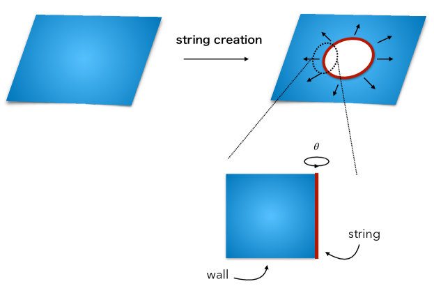
Figure 1: Schematic figure of the hybrid object consisting of a DW and cosmic string. The wall (blue) ends with the loop of the cosmic string (red). After nucleation of the string loop, it expands by eating the DW. Locally the string and wall are described by the straight long string in subsection 2.2 and the flat wall in subsection 2.1, respectively.

This hybrid defect appears in various cases. For instance, when the universe experiences a two-step SSB Kibble:1982dd , $G\to H\to 1$ with $\pi_{0}(H)\neq 0$ and $G$ being a simple group, the first SSB gives rise to the cosmic strings due to $\pi_{1}(G/H)=\pi_{0}(H)\neq 0$ and the second one does to the DWs. Another case is that the model has an approximate $U(1)$ symmetry that is explicitly broken by a tiny breaking parameter in the potential. This is nothing but the case of axion-like particles. In the both cases, the strings usually appear before the walls and form a network as well. The string network is here assumed to be diluted away by the cosmic inflation because otherwise the string network gets connected by the DWs and eventually decays by the wall tension well before the creation of the string loops. Since the DWs are not topologically stable in the both cases, they allow the string loops to be nucleated on them by quantum tunneling or thermal fluctuation, which are nothing but the hybrid defects stated above. We here present some concrete examples of particle physics models that can provide hybrid defects of DWs and cosmic strings. For other studies on hybrid defects of DWs and strings, see Refs. Kibble:1982dd ; Vilenkin:1982ks ; Everett:1982nm ; Preskill:1992ck ; Vilenkin:2000jqa ; Kawasaki:2013ae ; Eto:2023gfn .

Example 1: $SU(2)$ model

Let us consider two adjoint scalars and one doublet scalar charged under a $SU(2)$ symmetry, which can be either of gauge or global. When the adjoint scalars take VEVs, say, $\Delta^{(1)}=v_{\Delta}\sigma^{1}$ and $\Delta^{(2)}=v_{\Delta}\sigma^{2}$ ($\sigma^{a}$: the Pauli matrices), which break the $SU(2)$ symmetry down to the center $\mathbb{Z}_{2}$ symmetry, producing cosmic strings due to $\pi_{1}(SU(2)/\mathbb{Z}_{2})=\mathbb{Z}_{2}$. This string is called the $\mathbb{Z}_{2}$ string PhysRevLett.55.2398 because the winding number is characterized by $\mathbb{Z}_{2}$ charge. Due to the cosmic inflation, the produced strings are diluted away. Afterwards, the doublet scalar takes a VEV, so that the center $\mathbb{Z}_{2}$ symmetry is further broken into the trivial group $1$, producing DWs. Since the whole zero-th homotopy group is trivial, $\pi_{0}(SU(2))=0$, these DWs are not topologically stable but can decay by nucleation of the string loops.

Example 2: Axion-like particle

It is well known that models with axion-like particles can exhibit wall-string hybrid defects. Suppose that the model enjoys a global $U(1)$ symmetry, which is explicitly broken by a breaking term in the axion-like potential having a single potential minimum. This breaking term is not effective until some temperature (say, confinement scale of dark QCD) and thus cosmic strings appear when the $U(1)$ is spontaneously broken, being diluted away by the inflation. When the breaking term becomes effective, or equivalently, the axion potential is lifted except for the minimum point, the DWs are generated like sine-Gordon kinks. Since there is no discrete symmetry that is spontaneously broken, this DW is not topologically stable but allows the nucleation of string loops. This is nothing but the case of the axion DW of the DW number unity.

3 Gravitational waves from wall-string hybrid defects

3.1 Nucleation of string loop

The GW spectrum is calculated in this section. Here, we assume the cosmic strings to be produced in advance as stated in the last section. It gives a condition $v_{\mu}>v_{\sigma}$, where $v_{\mu/\sigma}$ represents the VEV of the fields constituting cosmic string/DW. Also, the DWs should not have boundary before the nucleation of the string loops, which requires the cosmic inflation to occur to dilute the strings away. Once the string loops are nucleated on DWs, they will expand faster and faster by eating the energy density of DWs Dunsky:2021tih . In this paper, the runaway case is assumed, i.e., the expansion is not affected by friction.

Each string loop expanding on the DW emits GW even for a flat DW configuration. This is because the quadrupole moment of the circular expanding loop is non-zero and depends on time, see Appendix A. Here, the curvature radius of DW is assumed to be larger than the typical size of the collided loops ($\beta^{-1}$ defined below) in order to approximate the DW as a planer object.

Unlike the purely quantum nucleation of the loops in Ref. Dunsky:2021tih , in which the nucleation rate does not depend on time, we instead consider a tunneling process due to the finite temperature, which allows us to assume the nucleation rate per unit area on the DWs to have the following expression

$$\Gamma(t)\simeq M^{3}\exp\left[-\frac{E_{\mathrm{crit.}}(\mu,\sigma,T_{\mathrm{temp}})}{T_{\mathrm{temp}}}\right]$$ (3.1)

where $M$ is some energy scale and $E_{\mathrm{crit.}}$ is the free energy of the nucleated loop on the DW with the critical size $R_{c}$. At the zero-temperature, $R_{c}$ is determined by Kibble:1982dd ; Preskill:1992ck

$$0 =\frac{d}{dR_{c}}\left(2\pi R_{c}\mu-\pi R_{c}^{2}\sigma\right)$$ (3.2)

$$\therefore\, E_{\mathrm{crit.}}(\mu,\sigma,T_{\mathrm{temp}}=0)=\frac{\pi\mu^{2}}{\sigma}$$ (3.3)

where $\mu$ and $\sigma$ are the tensions of string and DW. Taking into account the finite temperature correction, $\mu$, $\sigma$ and other model parameters depend on $T_{\mathrm{temp}}$, which makes it difficult to obtain the explicit expressions of $E_{\mathrm{crit.}}(\mu,\sigma,T_{\mathrm{temp}})$ and $\Gamma(t)$.

Inspired from the bubble nucleation process in the FOPT, we here simply assume the following expression

$$\Gamma(t)=\Gamma_{*}e^{\beta(t-t_{*})},$$ (3.4)

with $t_{*}$ being some fixed time typically around the decay time and $\Gamma_{*}$ the nucleation rate at $t=t_{*}$. We have ignored the quadratic and higher-order terms in the exponential. Ignoring the $T_{\mathrm{temp}}$-dependence in the prefactor of $\Gamma(t)$, the parameter $\beta$ is defined as

$$\beta=\partial_{t}\left.\frac{-E(\mu,\sigma,T_{\mathrm{temp}})}{T_{\mathrm{temp}}}\right|_{t=t_{*}}$$ (3.5)

and corresponds to the inverse of the duration of the nucleation process. Since it depends on microscopic parameters, it is calculable by performing the finite-temperature calculation in field theories once fixing a particle physics model. Nevertheless, it is beyond the scope of this paper, and hence we do not specify it here but leave it as a macroscopic free parameter.

In the following sections, we implicitly assume a relation $d_{\rm DW}^{-1}\gg\beta\gg H_{*}$, where $d_{\rm DW}$ is the width of the DWs and $H_{*}$ is the Hubble expansion rate at $t=t_{*}$. Since $\beta^{-1}$ is regarded as the typical size of the nucleation process, this relation is stating a reasonable assumption that it should be larger than the DW width and should not exceed the Hubble length. There is another necessary condition to perform our calculation. In order for the initial radius of the nucleated loops to be neglected, the relation $\beta^{-1}\gg R_{c}$ must be satisfied. When the finite-temperature correction is sub-leading, i.e., $R_{c}\simeq\mu/\sigma$, it is rewritten as

$$\beta^{-1}\gg\frac{\mu}{\sigma}\,,$$ (3.6)

which is typically satisfied in most cases.

3.2 Abundance of gravitational wave

Since we expect the production of GWs to complete in a short period compared to the Hubble time, the background metric is well approximated by the Minkowski one + linearized tensor perturbation,

$$ds^{2}=-dt^{2}+(\delta_{ij}+2h_{ij})dx^{i}dx^{j}+\mathcal{O}(h^{2})\,.$$ (3.7)

Also, the transverse-traceless gauge (TT gauge) is taken in the following calculation, $h_{ii}=0,\,\partial_{j}h_{ij}=0$. Our calculation refers to Ref. Jinno:2016vai . (See also Refs. Caprini:2007xq ; Jinno:2017fby .)

The gravitational wave is calculated from the linearized Einstein equation

$$\ddot{h}^{\rm TT}_{ij}(t,\vec{k})+\vec{k}^{2}h^{\rm TT}_{ij}(t,\vec{k})=8\pi G\Pi^{\rm TT}_{ij}(t,\vec{k}),$$ (3.8)

where $\Pi^{\rm TT}_{ij}(t,\vec{k})=K_{ijkl}(\hat{k})\Pi_{kl}(t,\vec{k})$ is the energy momentum tensor after the TT projection

$$K_{ijkl}(\hat{k})= P_{ik}(\hat{k})P_{jl}(\hat{k})-\frac{1}{2}P_{ij}(\hat{k})P_{kl}(\hat{k}),$$ (3.9)

$$P_{ij}(\hat{k})= \delta_{ij}-\hat{k}_{i}\hat{k}_{j},$$ (3.10)

and $\Pi_{kl}(t,\vec{k})$ is the energy momentum tensor in $k$-space. Here, hat represents the unit vector and the convention of Fourier transformation is taken as $\int d^{3}xe^{i\vec{k}\cdot\vec{x}}$ and $\int d^{3}k/(2\pi)^{3}e^{-i\vec{k}\cdot\vec{x}}$.

The Einstein equation is solved by using the method of Green’s function $G_{k}(t,t^{\prime})$

$$h^{\rm TT}_{ij}(t,\vec{k})=8\pi G\int_{-\infty}^{t}dt^{\prime}G_{k}(t,t^{\prime})\Pi^{\rm TT}_{ij}(t^{\prime},\vec{k}),$$ (3.11)

and the solution is $G_{k}(t,t^{\prime})=\sin{(k(t-t^{\prime}))}/k$. The gravitational wave propagates as a plane wave after its sources disappear at $t=t_{m}$. Then, the coefficients of plane gravitational wave are obtained by matching at time $t_{m}$ as

$$h^{\rm TT}_{ij}(t,\vec{k})= A_{ij}(\vec{k})\sin{(k(t-t_{m}))}+B_{ij}(\vec{k})\cos{(k(t-t_{m}))},$$ (3.12)

$$A_{ij}(\vec{k})= 8\pi G\int_{-\infty}^{t_{m}}dt^{\prime}\frac{\cos{(k(t_{m}-t^{\prime}))}}{k}\Pi^{\rm TT}_{ij}(t^{\prime},\vec{k}),$$ (3.13)

$$B_{ij}(\vec{k})= 8\pi G\int_{-\infty}^{t_{m}}dt^{\prime}\frac{\sin{(k(t_{m}-t^{\prime}))}}{k}\Pi^{\rm TT}_{ij}(t^{\prime},\vec{k}).$$ (3.14)

The total energy density of gravitational wave is taken as

$$\rho_{\rm GW}(t)= \frac{1}{8\pi G}\langle\dot{h}^{\rm TT}_{ij}(t,\vec{x})\,\dot{h}^{{\rm TT},ij}(t,\vec{x})\rangle_{T},$$ (3.15)

where $\langle\cdots\rangle_{T}$ represents the average over ensemble and time during a period of oscillation frequency.

Note that this ensemble average consists of an average over many nucleated loops and a spatial average of DW configurations. The equal-time correlator in the $k$-space becomes

$$\langle\dot{h}^{\rm TT}_{ij}(t,\vec{k}_{1})\,\dot{h}^{*{\rm TT},ij}(t,\vec{k}_{2})\rangle_{T}= {(8\pi G)^{2}}{}\int_{-\infty}^{\infty}dt_{1}\int_{-\infty}^{\infty}dt_{2}\langle\sum_{\{a,b\}}^{\rm walls}\Pi^{{\rm TT}}_{ij,a}(t_{1},\vec{k}_{1})\Pi^{*{\rm TT},ij}_{b}(t_{2},\vec{k}_{2})\rangle_{\rm ens}$$

$$\hskip 30.00005pt\times\int_{-T_{\rm osc}/2}^{T_{\rm osc}/2}\frac{dt^{\prime\prime}}{T_{\rm osc}}\cos(k_{1}(t^{\prime\prime}-t_{1}))\cos(k_{2}(t^{\prime\prime}-t_{2})),$$ (3.16)

where the time average over the oscillation frequency $T_{\rm osc}$ is shown explicitly and $\langle\cdots\rangle_{\rm ens}$ represents the ensemble average. The indices $a,b$ are introduced to label which DW the GW source (string loop) lies on. Here, the matching time is taken to $t_{m}\to\infty$ approximately because of the expression of nucleation rate Eq. (3.4). If the correlations between different DWs are negligible, the energy-momentum tensors inside the correlation function must lie on the same DW, i.e., $a=b$. Moreover, the spatial average gives the translational invariance leading to a delta function $\delta^{3}(\vec{k}_{1}-\vec{k}_{2})$. In the end, the equal-time correlator becomes

$$\langle\dot{h}^{\rm TT}_{ij}(t,\vec{k}_{1})\,\dot{h}^{*{\rm TT},ij}(t,\vec{k}_{2})\rangle_{T}= \frac{(8\pi G)^{2}}{2}\int_{-\infty}^{\infty}dt_{1}\int_{-\infty}^{\infty}dt_{2}\cos(k_{1}(t_{1}-t_{2}))$$

$$\hskip 30.00005pt\times(2\pi)^{3}\delta^{3}(\vec{k}_{1}-\vec{k}_{2})\Pi(t_{1},t_{2},k),$$ (3.17)

where

$$(2\pi)^{3}\delta^{3}(\vec{k}_{1}-\vec{k}_{2})\Pi(t_{1},t_{2},k)=\langle\sum_{a}^{\rm walls}\Pi^{\rm TT}_{ij,a}(t_{1},\vec{k}_{1})\Pi^{*{\rm TT},ij}_{a}(t_{2},\vec{k}_{2})\rangle_{\rm ens}\,.$$ (3.18)

Then, the energy density is rewritten as

$$\rho_{\rm GW}(t)= \frac{2G}{\pi}\int d(\ln k)\int_{-\infty}^{\infty}dt_{1}\int_{-\infty}^{\infty}dt_{2}k^{3}\cos{(k(t_{1}-t_{2}))}\Pi(t_{1},t_{2},k),$$ (3.19)

Hereafter, the thin string approximation $\ell_{s}\ll\beta^{-1}$ is taken, where $\ell_{s}$ is the thickness of string. Also, the envelope approximation Kosowsky:1991ua is used. Then, the energy momentum tensor (in the position space) of expanding and uncollided string loops are expressed as

$$T_{ij}(x)=\rho^{s}(x)\hat{n}(x-x_{N})_{i}\hat{n}(x-x_{N})_{j},$$ (3.20)

where the energy density is

$$\rho^{s}(x)=\pi r_{s}(t)^{2}\frac{\kappa\rho_{\rm re}}{2\pi r_{s}(t)\ell_{s}}\ \ \ \ (r_{s}(t)<|\vec{x}-\vec{x}_{N}|<r_{s}(t)+\ell_{s}),$$ (3.21)

and $\rho^{s}(x)=0$ otherwise. Here, $\rho_{\rm re}$ is the energy density released by expanding string loops. The efficiency factor, $\kappa$, is the fraction of kinetic energy density coming from the released energy density $\rho_{\rm re}$ Kamionkowski:1993fg . $x_{N}$ is the center of nucleation point of string loop, $\hat{n}(x)_{i}$ indicates the unit vector of direction $x_{i}$, and $r_{s}(t)$ is the radius of string loop. The initial radius is assumed to be negligible. The nucleated string loop will expand as a perfect circle until collision to other loops. Note that in contrast to the GW in FOPT, this expanding loops do radiate GWs even before the collision. This can be seen from the fact that the quadrupole moment of the energy density of the single loop does not vanish. See Appendix A for the explicit calculation.

The energy fraction of GW is

$$\Omega_{\rm GW}(t_{*},k_{*})\equiv\frac{1}{\rho_{\rm tot}(t_{*})}\frac{d\rho_{\rm GW}(k_{*})}{d\ln k_{*}},$$ (3.22)

where $\rho_{\rm tot}(t_{*})=\rho_{\rm re}+\rho_{\rm pla}(t_{*})$ is the total energy density and $\rho_{\rm pla}(t_{*})$ is the plasma energy density in the background. The gravitational wave abundance $\Omega_{\rm GW}(t_{*},k_{*})$ is rewritten by defining a dimensionless spectrum function $\Delta(k/\beta)$ as

$$\Omega_{\rm GW}(t_{*},k_{*})= \kappa^{2}\left(\frac{H_{*}}{\beta}\right)^{2}\left(\frac{\alpha(t_{*})}{1+\alpha(t_{*})}\right)^{2}\Delta(k_{*}/\beta),$$ (3.23)

$$\Delta(k/\beta)= \frac{3}{8\pi G}\frac{\beta^{2}\rho_{\rm tot}(t)}{\kappa^{2}\rho_{\rm re}^{2}}\Omega_{\rm GW}(t,k),$$ (3.24)

$$= \frac{3}{4\pi^{2}}\frac{\beta^{2}k^{3}}{\kappa^{2}\rho_{\rm re}^{2}}\int_{-\infty}^{\infty}dt_{1}\int_{-\infty}^{\infty}dt_{2}\cos{(k(t_{1}-t_{2}))}\Pi(t_{1},t_{2},k),$$ (3.25)

where $H_{*}^{2}=8\pi G\rho_{\rm tot}(t_{*})/3$, $\alpha(t_{*})=\rho_{\rm re}/\rho_{\rm pla}(t_{*})$, and $\Pi(t_{1},t_{2},k)$ can be explicitly rewritten as

$$\Pi(t_{1},t_{2},k)= K_{ijkl}(\hat{k})K_{ijmn}(\hat{k})\int d^{3}re^{i\vec{k}\cdot\vec{r}}\langle T_{kl}T_{mn}\rangle_{\rm ens}(t_{1},t_{2},r)\,.$$ (3.26)

Here, $r=|\vec{r}_{1}-\vec{r}_{2}|$ is the spatial distance between two evaluation points. We have omitted the labels of the DWs for notational simplicity. As seen below, $\Delta$ depends on $k$ only through a form $k/\beta$. Note that the runaway case is assumed and the initial radius of the nucleated loops is ignored. Therefore, the speed of expanding string loop is approximated by that of light.

The ensemble average $\langle T_{kl}T_{mn}\rangle_{\rm ens}(t_{1},t_{2},r)$ has spatial dependence only through the distance $r$ thanks to the homogeneity and isotropy. The value of energy momentum tensor at a space-time point $(t_{i},\vec{r}_{i})$ is determined by the time evolution of the expanding string loops that move with the speed of light. Therefore, the calculation reduces to the geometric consideration determined by light cone structures.

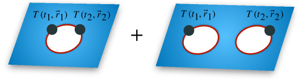
Figure 2: Illustration of two contributions to the two-point correlation function of the energy-momentum tensors. The two evaluation points can lie on one string loop (left) or on two loops (right). Although we take $t_{1}=t_{2}$ for the illustration in the figure, they can be different in general. Note that the GWs can be radiated even when the loops do not yet collide to the other loops.

There are two contributions of energy momentum tensors depending on where the evaluation points of the energy-momentum tensors lies. One comes from a single expanding string loop, in which they lie on the same expanding loop whereas the other one come from two expanding string loops, in which they lie on different expanding loops. See Fig. 2 for the illustration. Thus we can divide the correlation function into two parts as

$$\langle T_{kl}T_{mn}\rangle_{\rm ens}(t_{1},t_{2},r)=\langle T_{kl}T_{mn}\rangle_{\rm ens}^{\rm single}(t_{1},t_{2},r)+\langle T_{kl}T_{mn}\rangle_{\rm ens}^{\rm double}(t_{1},t_{2},r).$$ (3.27)

Correspondingly, $\Delta(k_{*}/\beta)$ is also divided as

$$\Delta(k/\beta) =\Delta^{\mathrm{single}}(k/\beta)+\Delta^{\mathrm{double}}(k/\beta)$$ (3.28)

with

$$\Delta^{\mathrm{single}}(k/\beta)\equiv \frac{3}{4\pi^{2}}\frac{\beta^{2}k^{3}}{\kappa^{2}\rho_{\rm re}^{2}}\int_{-\infty}^{\infty}dt_{1}\int_{-\infty}^{\infty}dt_{2}\cos{(k(t_{1}-t_{2}))}\Pi(t_{1},t_{2},k)^{\rm single}$$ (3.29)

$$\Delta^{\mathrm{double}}(k/\beta)\equiv \frac{3}{4\pi^{2}}\frac{\beta^{2}k^{3}}{\kappa^{2}\rho_{\rm re}^{2}}\int_{-\infty}^{\infty}dt_{1}\int_{-\infty}^{\infty}dt_{2}\cos{(k(t_{1}-t_{2}))}\Pi(t_{1},t_{2},k)^{\mathrm{double}}\,.$$ (3.30)

While $\langle T_{kl}T_{mn}\rangle_{\rm ens}^{\rm single}(t_{1},t_{2},r)$ contains the integration over one nucleation point corresponding to the single expanding loop, $\langle T_{kl}T_{mn}\rangle_{\rm ens}^{\rm double}(t_{1},t_{2},r)$ contains the integration over two nucleation points as seen below. It is shown later that the contribution from two expanding string loops dominates the gravitational wave spectrum. Thus we first consider the case of two expanding string loops. Although the two-loop contribution contains that of uncollided expanding string loops, we call this contribution a double string-loop contribution following the terminology introduced in Ref. Jinno:2016vai .

3.3 Contribution from two expanding string loops

3.3.1 Ensemble average

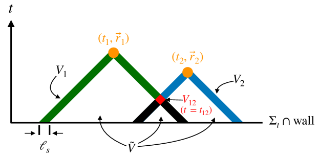
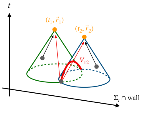
Figure 3: Past light cones of evaluation points $(t_{i},\vec{r}_{i})$ with the width $\ell_{s}$. (top:) The Horizontal direction represents the two dimensional intersection of the DW and the constant-time hypersurface $\Sigma_{t}$. Nucleation points of expanding string loops must be on the surface of the past light cones with the width $\ell_{s}$ because of the envelope approximation. For two-loop contribution, one nucleation point must be in the $2+1$ dimensional green colored region $V_{1}$ and the other point must be in the blue colored one $V_{2}$. For single-loop contribution, the nucleation point must be in the intersection of the two light cones $V_{12}$, shown as the red region. The region inside of the two light cones is denoted by $\tilde{V}$, which includes the black region. (bottom:) $2+1$ dimensional version of the top figure. Gray blobs indicate the nucleation points and arrows represent how the expanding string loops reach the evaluation points. The red arch indicates $V_{12}$.

To proceed our calculation, we need some geometric consideration. Fig. 3 shows the notation of quantities for the past light cones of evaluation points $(t_{1},\vec{r}_{1})$ and $(t_{2},\vec{r}_{2})$. As stated above, the energy-momentum tensor $T_{ij}$ lies only on the DW since the loops expand on it, which results in that it is sufficient to consider the light cones in $2+1$ dimensional spacetime ignoring the direction orthogonal to the DW. Note that the spatial integration in Eq. (3.26) should be performed in the three dimensions.

The ensemble average is given by
(i) the value of energy momentum tensors which is on the DW, $T_{kl}(t_{1},\vec{r})T_{mn}(t_{2},\vec{r})$
(ii-a) a probability that two evaluation points are on the DW, i.e., no loop is nucleated inside the two past light cones, $P(t_{1},t_{2},r)$ (envelope approximation)
(ii-b) a probability that each of two string loops is nucleated in the $2+1$ dimensional green region $V_{1}$ and the blue region $V_{2}$ in Fig. 3, $\int dt_{n1}dt_{n2}\int_{A_{1}}d^{2}z_{1}\int_{A_{2}}d^{2}z_{2}\Gamma(t_{n1})\Gamma(t_{n2})$
(ii-c) a probability that the two evaluation points lie on the randomly distributed DW, $C_{\rm DW}(r)$.

Here, the regions $V_{1}$ and $V_{2}$ correspond to the surfaces of the past light cones of the two evaluation points with the width $\ell_{s}$, in which the black region in Fig. 3 is excluded by the condition (ii-a). The integral $\int_{A_{i}}$ is over the area $A_{i}$ which represents the area of the intersection among $V_{i}$, the constant-time hypersurface $\Sigma_{t}$, and the DW. (See Fig. 4.) The time variable $t_{ni}$ represents the time of the loop nucleation point.

Then, the ensemble average from two expanding string loops is given by

$$\langle T_{kl}T_{mn}\rangle_{\rm ens}^{\rm double}(t_{1},t_{2},r)=C_{\rm DW}(r)P(t_{1},t_{2},r) \int_{-\infty}^{t_{1}}dt_{n1}\Gamma(t_{n1})\int_{A_{1}}d^{2}z_{1}T_{kl}(t_{1},\vec{r})$$

$$\times \int_{-\infty}^{t_{2}}dt_{n2}\Gamma(t_{n2})\int_{A_{2}}d^{2}z_{2}T_{mn}(t_{2},\vec{r}),$$ (3.31)

where Eq. (3.20) is used. The envelope approximation allows the energy-momentum tensor to have a non-zero value only when the two evaluation points are spacelike $r>|t_{d}|$, where $t_{d}=t_{1}-t_{2}$. Note that the two integrations about the expanding string loops 1 and 2 can be factorized into each integration as is shown in Eq. (3.3.1) because they depend on different nucleation time $t_{n1}$ and $t_{n2}$. Each component is calculated in the following.

3.3.2 Random configuration of domain walls

Let us obtain a probability that two points $\vec{r}_{1},\vec{r}_{2}$ lie on a DW that is randomly distributed in the Hubble patch. As the first step, let us assume that there exists only one DW within one Hubble patch. We can rephrase this problem as the probability that a needle (or segment) that is randomly distributed in the three-dimensional space lies on a fixed DW on $y=0$. This is similar to the 3D version of Buffon’s needle. Let the $y$ coordinate of the center of the needle be $h$ and two angles be $\theta\in[0,\pi/2)$ (angle from the DW) and $\phi\in[0,\pi)$ (angle around $y$ axes). The density probability function of $h,\theta,\phi$ are given as

$$f_{h}(h) =\frac{1}{d_{H}}$$ (3.32)

$$f_{\theta}(\theta) =\sin\theta$$ (3.33)

$$f_{\phi}(\phi) =\frac{1}{\pi}\,,$$ (3.34)

where $d_{H}$ is the Hubble length $d_{H}=1/H_{\ast}$. The two endpoints lie on the DW with its width $d_{\rm DW}$ if and only if relations

$$\left|h\pm\frac{r}{2}\cos\theta\right|\leq\frac{d_{\rm DW}}{2}$$ (3.35)

are satisfied for the both signs $\pm$. Thus, we get the probability as

$$C_{\rm DW}^{(0)}(r) =\int_{0}^{\pi}d\phi\int_{\cos^{-1}(d_{\rm DW}/r)}^{\pi/2}d\theta\int_{-\frac{d_{\rm DW}}{2}+\frac{r}{2}\cos\theta}^{\frac{d_{\rm DW}}{2}-\frac{r}{2}\cos\theta}dh\,\frac{\sin\theta}{\pi d_{H}}$$ (3.36)

$$=\frac{d_{\rm DW}^{2}}{2rd_{H}}.$$ (3.37)

Then, taking into account the number of the DWs $N_{\mathrm{walls}}$ in the Hubble patch, the full probability $C_{\rm DW}(r)$ is expressed as

$$C_{\rm DW}(r)= N_{\rm walls}C_{\rm DW}^{(0)}(r),$$ (3.38)

$$= N_{\rm walls}\frac{d_{\rm DW}^{2}}{{2rd_{H}}}.$$ (3.39)

The value of $N_{\rm walls}$ depends on cosmological scenarios which will be argued in Sec. 4.

3.3.3 Probability of domain wall to remain

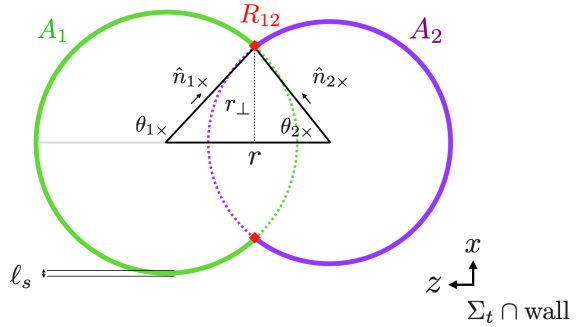
Figure 4: Figure of geometry for calculation on the constant-time hypersurface $\Sigma_{t}$. See also Fig. 3.

The probability $P(t_{1},t_{2},r)$ is obtained by calculating the $2+1$ dimensional volume $\tilde{V}$ of the union of the inside of the two past light cones for the evaluation points shown in Fig. 3. The volume $\tilde{V}$ is obtained by integrating with respect to time the area of the union of the inside of the two circles shown in Fig. 4.

Dividing $\tilde{V}$ into infinitesimal $2+1$ dimensional regions labeled by $i$, $\tilde{V}^{i}$, the probability that no loop is nucleated in $\tilde{V}$ is expressed as

$$P(t_{1},t_{2},r)= \prod_{i}(1-\Gamma(t)d\tilde{V}^{i}),$$ (3.40)

$$= e^{-I(x_{1},x_{2})}\,,$$ (3.41)

with

$$I(x_{1},x_{2})\equiv\int_{\tilde{V}}d^{3}z\,\Gamma(t)\,.$$ (3.42)

To proceed the calculation, one should note that the two circles on $\Sigma_{t}$ can be either of overlapped or not depending on $t$. The overlapped region exists when $-\infty<t<t_{12}$, where the time $t_{12}\equiv(t_{1}+t_{2}-r)/2$ represents when the two past light cones meet. Then, the above expression is calculated as

$$I(x_{1},x_{2})= \Gamma(T)\mathcal{I}(r,t_{d}),$$ (3.43)

$$\mathcal{I}(r,t_{d})= \frac{1}{2\beta^{3}}\left[8\pi\cosh{\left(\frac{\beta t_{d}}{2}\right)}+\beta^{2}r\sqrt{r^{2}-t_{d}^{2}}K_{1}\left(\frac{\beta r}{2}\right)\right]$$

$$-\frac{1}{4}\int_{-\infty}^{-r/2}dt_{T}\,e^{\beta t_{T}}\left[(2t_{T}-t_{d})^{2}\left(\pi-\cos^{-1}\left(\frac{r^{2}-2t_{d}t_{T}}{r(2t_{T}-t_{d})}\right)\right)\right.$$

$$\left.+(2t_{T}+t_{d})^{2}\left(\pi-\cos^{-1}\left(\frac{r^{2}+2t_{d}t_{T}}{r(2t_{T}+t_{d})}\right)\right)\right],$$ (3.44)

where $K_{1}(x)$ is the modified Bessel function of second kind. The above expression of $\mathcal{I}(r,t_{d})$ is invariant under $t_{d}\to-t_{d}$. Here, $T\equiv(t_{1}+t_{2})/2$ is defined. The integration in Eq. (3.44) is well fitted by $e^{-r/2-t_{d}}$ multiplied with the polynomials of $r$ and $t_{d}$ up to fifth orders.

3.3.4 Evaluation of $\Delta^{\mathrm{double}}$

Consider a dynamics of two expanding string loops in constant-time hypersurface $\Sigma_{t_{1}}$ and $\Sigma_{t_{2}}$. The areas on which the string loops 1(2) can be nucleated are (See Fig. 4.)

$$\int_{A_{1}}d^{2}z_{1}= \ell_{s}\begin{cases}\int_{-\theta_{1\times}}^{\theta_{1\times}}r_{1\times}(t_{n1})d\theta_{1}&\ \ \ ({\rm for}-\infty<t_{n1}<-r/2)\\ 2\pi r_{1\times}(t_{n1})&\ \ \ ({\rm for}-r/2<t_{n1}<t_{1})\end{cases},$$ (3.45)

$$\int_{A_{2}}d^{2}z_{2}= \ell_{s}\begin{cases}\int_{\theta_{2\times}}^{2\pi-\theta_{2\times}}r_{2\times}(t_{n2})d\theta_{2}&({\rm for}-\infty<t_{n2}<-r/2)\\ 2\pi r_{2\times}(t_{n2})&({\rm for}-r/2<t_{n2}<t_{2})\end{cases}.$$ (3.46)

Here, $\times$ indicates the overlapped points of past light cones shown in Fig. 4. $r_{1(2)}(t_{n})=t_{1(2)}-t_{n}$ is the radius of nucleated string loop. Remind that the initial radius of string loop is neglected. The binomial tensors are written as

$$\int_{A_{1}}d^{2}z_{1}\int_{A_{2}}d^{2}z_{2}T_{kl}(t_{1},\vec{r})T_{mn}(t_{2},\vec{r})= \left(\frac{\kappa\rho_{\rm re}}{2}\right)^{2}\int_{-\theta_{1\times}}^{\theta_{1\times}}d\theta_{1}r_{1\times}^{2}(t_{n1})\hat{n}_{1,k}(t_{n1})\hat{n}_{1,l}(t_{n1})$$

$$\ \ \times\int_{\theta_{2\times}}^{2\pi-\theta_{2\times}}d\theta_{2}r_{2\times}^{2}(t_{n2})\hat{n}_{2,m}(t_{n2})\hat{n}_{2,n}(t_{n2}),$$ (3.47)

for $-\infty<t_{n1(2)}<-r/2$. For $-r/2<t_{n1(2)}<t_{1(2)}$, which means that the circles do not have overlap, the corresponding expression is obtained by just taking $\theta_{1\times}=\pi$ and $\theta_{2\times}=0$ in the above expression. Here, $\hat{n}_{i,k}$ is the unit vector for expanding string loop $i$ with direction $k$. The above expression does not depend on $\ell_{s}$.

The DW plane is set as $xz$ plane in the coordinate system. Then, the vector $\vec{r}$ is on the $xz$ plane and the direction of $\vec{r}=\vec{r}_{1}-\vec{r}_{2}$ can be taken as the $z$ axis. The unit vector of the energy-momentum tensor is taken as $\hat{n}_{1(2)\times}=(\sin\theta_{1(2)\times},0,\cos\theta_{1(2)\times})$. The vector $\vec{k}$ is taken as $\vec{k}=k(\sin{\theta_{kr}}\cos{\phi_{kr}},\sin{\theta_{kr}}\sin{\phi_{kr}},\cos{\theta_{kr}})$. Then, the integral $\int d^{3}r$ in Eq. (3.26) is written as $\int d^{3}r=\int_{0}^{\infty}r^{2}dr\int_{-1}^{1}dc_{kr}\int_{0}^{2\pi}d\phi_{kr}$, where $c_{rk}=\hat{k}\cdot\hat{r}=\cos{\theta_{kr}}$. By using $T=(t_{1}+t_{2})/2$ and $t_{d}=t_{1}-t_{2}$, the variables $t_{1(2)}$ are eliminated, i.e., $t_{1/2}=T\pm t_{d}/2$.

Then, the TT projection becomes

$$\int_{0}^{2\pi}d\phi_{kr}K_{ijkl}(\hat{k})K_{ijmn}(\hat{k})\langle T_{kl}T_{mn}\rangle_{\rm ens}^{\rm double}(t_{1},t_{2},r)$$

$$= \frac{\pi}{4}\kappa^{2}\rho_{\rm re}^{2}C_{\rm DW}P(t_{1},t_{2},r)\Gamma(T)^{2}\int_{-\infty}^{t_{d}/2}dt_{1T}\int_{-\infty}^{-t_{d}/2}dt_{2T}r_{1\times}^{2}r_{2\times}^{2}$$

$$\times e^{\beta(t_{1T}+t_{2T})}\left[\frac{1}{2}G_{0}+\frac{1}{4}(1-c_{rk}^{2})G_{1}+\frac{1}{16}(1-c_{rk}^{2})^{2}G_{2}\right],$$ (3.48)

where $t_{iT}\equiv t_{ni}-T$, and

$$G_{0}(\theta_{1\times},\theta_{2\times}) =2(\theta_{1\times}-\sin\theta_{1\times}\cos\theta_{1\times})(\pi-\theta_{2\times}+\sin\theta_{2\times}\cos\theta_{2\times}),$$ (3.49)

$$G_{1}(\theta_{1\times},\theta_{2\times}) =-2G_{0}(\theta_{1\times},\theta_{2\times}),$$ (3.50)

$$G_{2}(\theta_{1\times},\theta_{2\times}) =6\theta_{1\times}(\pi-\theta_{2\times})-10\theta_{1\times}\sin\theta_{2\times}\cos\theta_{2\times}+10(\pi-\theta_{2\times})\sin\theta_{1\times}\cos\theta_{1\times}$$

$$\hskip 20.00003pt-38\sin\theta_{1\times}\cos\theta_{1\times}\sin\theta_{2\times}\cos\theta_{2\times}.$$ (3.51)

The functions, $G_{i}(\theta_{1\times},\theta_{2\times})$, have a symmetry of exchange between $\theta_{1\times}$ and $\bar{\theta}_{2\times}=\pi-\theta_{2\times}$. Here, $\cos\theta_{1\times}=-[r^{2}+r_{1}(t_{n1})^{2}-r_{2}(t_{n1})^{2}]/[2r_{1}(t_{n1})r]$ and $\cos\theta_{2\times}=[r^{2}+r_{2}(t_{n2})^{2}-r_{1}(t_{n2})^{2}]/[2r_{2}(t_{n2})r]$, see Fig. 4. Then, the spectrum function $\Delta^{\rm double}(k/\beta)$ is obtained as

$$\Delta^{\rm double}(k/\beta)= \frac{3}{64\pi}\beta k^{3}\int_{0}^{\infty}dt_{d}\cos(kt_{d})\int_{t_{d}}^{\infty}dr\frac{r^{2}C_{\rm DW}(r)}{\mathcal{I}(r,t_{d})^{2}}$$

$$\times\int_{-\infty}^{t_{d}/2}dt_{1T}\int_{-\infty}^{-t_{d}/2}dt_{2T}e^{\beta(t_{1T}+t_{2T})}\left[\left(j_{0}(kr)-2\frac{j_{1}(kr)}{kr}\right)G_{0}^{\prime}+\frac{j_{2}(kr)}{(kr)^{2}}G_{2}^{\prime}\right],$$ (3.52)

where, $j_{0}(x)=\frac{1}{2}\int_{-1}^{1}dc\,e^{icx}$, $j_{1}(x)/x=\frac{1}{4}\int_{-1}^{1}dc(1-c^{2})e^{icx}$, and $j_{2}(x)/x^{2}=\frac{1}{16}\int_{-1}^{1}dc(1-c^{2})^{2}e^{icx}$ are the spherical Bessel function,

$$G_{0}^{\prime}(r,t_{d},t_{1T},t_{2T})= \left[g_{a}^{\prime}(r,t_{d},t_{1T})+g_{b}^{\prime}(r,t_{d},t_{1T})\right]\left[g_{a}^{\prime}(r,-t_{d},t_{2T})+g_{b}^{\prime}(r,-t_{d},t_{2T})\right],$$ (3.53)

$$G_{2}^{\prime}(r,t_{d},t_{1T},t_{2T})= 3g_{a}^{\prime}(r,t_{d},t_{1T})g_{a}^{\prime}(r,-t_{d},t_{2T})+19g_{b}^{\prime}(r,t_{d},t_{1T})g_{b}^{\prime}(r,-t_{d},t_{2T})$$

$$-5g_{a}^{\prime}(r,t_{d},t_{1T})g_{b}^{\prime}(r,-t_{d},t_{2T})-5g_{b}^{\prime}(r,t_{d},t_{1T})g_{a}^{\prime}(r,-t_{d},t_{2T}),$$ (3.54)

and

$$g_{a{\rm}}^{\prime}(r,t_{d},t_{1T})= \begin{cases}(-2t_{1T}+t_{d})^{2}\cos^{-1}\left(\frac{r^{2}-2t_{1T}t_{d}}{r(2t_{1T}-t_{d})}\right)&\ \ \ (-\infty<t_{1T}<-r/2)\\ \pi(-2t_{1T}+t_{d})^{2}&\ \ \ (-r/2<t_{1T}<t_{d}/2)\end{cases},$$ (3.55)

$$g_{b{\rm}}^{\prime}(r,t_{d},t_{1T})= \begin{cases}\frac{r^{2}-2t_{1T}t_{d}}{r^{2}}\sqrt{(4t_{1T}^{2}-r^{2})(r^{2}-t_{d}^{2})}&\ \ \ \ (-\infty<t_{1T}<-r/2)\\ 0&\ \ \ \ (-r/2<t_{1T}<t_{d}/2)\end{cases}.$$ (3.56)

Here, the relation $r>|t_{d}|$, a symmetry of $G_{i}^{\prime}$ under $t_{d}\to-t_{d}$, and a formula of $\int_{0}^{\infty}dzz^{n-1}e^{-xz}=(n-1)!/x^{n}$ with $z=e^{y}$ are used.

The integral with respect to $t_{1(2)T}$ is calculated analytically for some terms. The above functions are redefined as

$$g_{a,{\rm ov}}^{\prime\prime}(r,t_{d})= \int_{-\infty}^{-r/2}dt_{1T}e^{\beta t_{1T}}g_{a{\rm}}^{\prime}(r,t_{d},t_{1T}),$$ (3.57)

$$g_{a,{\rm non}}^{\prime\prime}(r,t_{d})= \int_{-r/2}^{t_{d}/2}dt_{1T}e^{\beta t_{1T}}g_{a{\rm}}^{\prime}(r,t_{d},t_{1T})$$ (3.58)

$$= \frac{\pi}{\beta^{3}}e^{-\beta r/2}\left[8(-1+e^{\beta(r+t_{d})/2})-\beta(r+t_{d})\left\{4+\beta(r+t_{d})\right\}\right],$$ (3.59)

$$g_{b,{\rm ov}}^{\prime\prime}(r,t_{d})= \int_{-\infty}^{-r/2}dt_{1T}e^{\beta t_{1T}}g_{b{\rm}}^{\prime}(r,t_{d},t_{1T})$$ (3.60)

$$= \frac{\sqrt{r^{2}-t_{d}^{2}}}{\beta}\left[rK_{1}\left(\frac{\beta r}{2}\right)+t_{d}K_{2}\left(\frac{\beta r}{2}\right)\right]\,,$$ (3.61)

where the subscripts “$\mathrm{ov}$” and “$\mathrm{non}$” mean the integral region in which the two past light cones are overlapped and not (non overlapped), respectively. Then, the spectrum function $\Delta^{\rm double}(k/\beta)$ becomes

$$\Delta^{\rm double}(k/\beta)= \frac{3}{64\pi}\beta k^{3}\int_{0}^{\infty}dt_{d}\cos(kt_{d})\int_{t_{d}}^{\infty}dr\frac{r^{2}C_{\rm DW}(r)}{\mathcal{I}(r,t_{d})^{2}}$$

$$\times\left[\left(j_{0}(kr)-2\frac{j_{1}(kr)}{kr}+3\frac{j_{2}(kr)}{(kr)^{2}}\right)\right.$$

$$\ \ \times\left(g_{a,{\rm ov}}^{\prime\prime}(r,t_{d})+g_{a,{\rm non}}^{\prime\prime}(r,t_{d})\right)\left(g_{a,{\rm ov}}^{\prime\prime}(r,-t_{d})+g_{a,{\rm non}}^{\prime\prime}(r,-t_{d})\right)$$

$$\ \ +\left(j_{0}(kr)-2\frac{j_{1}(kr)}{kr}-5\frac{j_{2}(kr)}{(kr)^{2}}\right)$$

$$\ \ \times\left[\left(g_{a,{\rm ov}}^{\prime\prime}(r,t_{d})+g_{a,{\rm non}}^{\prime\prime}(r,t_{d})\right)g_{b,{\rm ov}}^{\prime\prime}(r,-t_{d})+g_{b,{\rm ov}}^{\prime\prime}(r,t_{d})\left(g_{a,{\rm ov}}^{\prime\prime}(r,-t_{d})+g_{a,{\rm non}}^{\prime\prime}(r,-t_{d})\right)\right]$$

$$\left.+\left(j_{0}(kr)-2\frac{j_{1}(kr)}{kr}+19\frac{j_{2}(kr)}{(kr)^{2}}\right)g_{b,{\rm ov}}^{\prime\prime}(r,t_{d})g_{b,{\rm ov}}^{\prime\prime}(r,-t_{d})\right].$$ (3.62)

This is the main result of the analytic formula for $\Delta^{\mathrm{double}}$.

The remaining integrals are performed numerically. However, there are simply oscillating terms at large $r$ whose integration does not converge as shown in the following. The term $g_{a,{\rm non}}^{\prime\prime}(r,t_{d})g_{a,{\rm non}}^{\prime\prime}(r,-t_{d})$ is separated as

$$g_{a,{\rm non}}^{\prime\prime}(r,t_{d})g_{a,{\rm non}}^{\prime\prime}(r,-t_{d})= g_{\rm IR}(r,t_{d})+g_{{\rm conv}}(r,t_{d}),$$ (3.63)

where

$$g_{{\rm IR}}(r,t_{d})= 64\pi^{2},$$ (3.64)

$$g_{{\rm conv}}(r,t_{d})= \pi^{2}e^{-r}\left[(8+4r+r^{2})^{2}-2r(4+r)t_{d}^{2}+t_{d}^{4}\right]$$

$$-16\pi^{2}e^{-\frac{r}{2}}\left((8+4r+r^{2}+t_{d}^{2})\cosh{\frac{t_{d}}{2}}-2(2+r)t_{d}\sinh{\frac{t_{d}}{2}}\right).$$ (3.65)

Note that $g_{{\rm conv}}$ exponentially decays at $r\to\infty$ whereas $g_{{\rm IR}}$ is a constant and not well-behaved. Thus let us take a closer look at the contribution from $g_{{\rm IR}}(r,t_{d})$, which is further separated as

$$\left.\Delta^{\mathrm{double}}\right|_{g_{{\rm IR}}\text{ part}}=\Delta^{\rm double}_{{\rm IR0}}+\Delta^{\rm double}_{{\rm IR12}}$$ (3.66)

with

$$\Delta^{\rm double}_{{\rm IR0}}(k/\beta)= {3\pi}{}\beta k^{3}\int_{0}^{\infty}dt_{d}\cos(kt_{d})\int_{t_{d}}^{\infty}dr\frac{r^{2}C_{\rm DW}(r)}{\mathcal{I}(r,t_{d})^{2}}j_{0}(kr),$$ (3.67)

$$\Delta^{\rm double}_{{\rm IR12}}(k/\beta)= {3\pi}{}\beta k^{3}\int_{0}^{\infty}dt_{d}\cos(kt_{d})\int_{t_{d}}^{\infty}dr\frac{r^{2}C_{\rm DW}(r)}{\mathcal{I}(r,t_{d})^{2}}\left[-2\frac{j_{1}(kr)}{kr}+3\frac{j_{2}(kr)}{(kr)^{2}}\right].$$ (3.68)

One can see that the second term $\Delta^{\rm double}_{{\rm IR12}}$ is a convergent integral thanks to decaying polynomials of $r$ while the first term $\Delta^{\rm double}_{{\rm IR0}}(k/\beta)$ contains simply oscillating terms at large $r$. Indeed, at $r\to\infty$, its integrand is approximated as

$$\Delta^{\rm double}_{{\rm IR0}}(k/\beta)\overset{r\to\infty}{\to} ~{}{3\pi}{}\beta k^{3}\int_{0}^{\infty}dt_{d}\cos(kt_{d})\int_{t_{d}}^{\infty}drr^{2}C_{\rm DW}(r)\frac{1}{\mathcal{I}(\infty,t_{d})^{2}}j_{0}(kr),$$ (3.69)

$$= \frac{3N_{\rm walls}d_{\rm DW}^{2}H_{*}k^{2}}{32\pi}\int_{0}^{\infty}dr_{t_{d}}\left[\left(1+\frac{2\pi k/\beta}{\sinh\frac{2\pi k}{\beta}}\right)\sin(kr_{t_{d}})+\beta^{-1}k\chi(k/\beta)\cos(kr)\right],$$ (3.70)

where $r_{t_{d}}\equiv r-t_{d}$ and

$$\chi(k/\beta)= H_{ik/\beta}+H_{-ik/\beta}-H_{-\frac{1}{2}+ik/\beta}-H_{-\frac{1}{2}-ik/\beta},$$ (3.71)

$$H_{y}= \int_{0}^{1}dx\frac{1-x^{y}}{1-x}.$$ (3.72)

Here, $H_{y}$ is the harmonic number of integral representation for complex plane. Introducing an IR cutoff $L$ for the numerical integration, it gives

$$\Delta^{\rm double}_{{\rm IR0}}(k/\beta)\overset{r\to\infty}{\to} ~{}\frac{3N_{\rm walls}d_{\rm DW}^{2}H_{*}k}{32\pi}\left[\left(1+\frac{2\pi k/\beta}{\sinh\frac{2\pi k}{\beta}}\right)(1-\cos(kL))+\beta^{-1}k\chi(k/\beta)\sin(kL)\right].$$ (3.73)

Therefore, we rewrite the divergent integral $\Delta^{\rm double}_{{\rm IR0}}(k/\beta)$ using the following trick:

$$\Delta^{\rm double}_{{\rm IR0}}(k/\beta)= {3\pi}{}\beta k^{3}\int_{0}^{\infty}dt_{d}\cos(kt_{d})\int_{t_{d}}^{\infty}drr^{2}C_{\rm DW}(r)\left(\frac{1}{\mathcal{I}(r,t_{d})^{2}}-\frac{1}{\mathcal{I}(\infty,t_{d})^{2}}+\frac{1}{\mathcal{I}(\infty,t_{d})^{2}}\right)j_{0}(kr)$$ (3.74)

$$= {3\pi}{}\beta k^{3}\int_{0}^{\infty}dt_{d}\cos(kt_{d})\int_{t_{d}}^{\infty}drr^{2}C_{\rm DW}(r)\left(\frac{1}{\mathcal{I}(r,t_{d})^{2}}-\frac{1}{\mathcal{I}(\infty,t_{d})^{2}}\right)j_{0}(kr)$$

$$+\frac{3N_{\rm walls}d_{\rm DW}^{2}H_{*}k}{32\pi}\left[\left(1+\frac{2\pi k/\beta}{\sinh\frac{2\pi k}{\beta}}\right)(1-\cos(kL))+\beta^{-1}k\chi(k/\beta)\sin(kL)\right]\,.$$ (3.75)

Thanks to the subtraction within the parenthesis in the first line, the numerical integration with respect to $r$ is well convergent and easy to evaluate. On the other hand, this expression explicitly depends on the IR cutoff $L$. Note that the IR cutoff $L$ corresponds to the curvature radius of the DW, beyond which our approximation of the DW to be planar is not reliable. Therefore its appearance does not necessarily mean the inconsistency of the calculation. We here take the average over $L$ so that the final results does not depend on $L$. Thus, we get

$$\Delta^{\rm double}_{{\rm IR0}}(k/\beta)= {3\pi}{}\beta k^{3}\int_{0}^{\infty}dt_{d}\cos(kt_{d})\int_{t_{d}}^{\infty}drr^{2}C_{\rm DW}(r)\left(\frac{1}{\mathcal{I}(r,t_{d})^{2}}-\frac{1}{\mathcal{I}(\infty,t_{d})^{2}}\right)j_{0}(kr)$$

$$+\frac{3N_{\rm walls}d_{\rm DW}^{2}H_{*}k}{32\pi}\left(1+\frac{2\pi k/\beta}{\sinh\frac{2\pi k}{\beta}}\right).$$ (3.76)

One may consider that this prescription of $L$ looks somewhat ad hoc. Nevertheless, it is justified by the causality argument. If a different choice of $L$ were taken, $\Delta^{\mathrm{double}}(k/\beta)$ and hence the final result of $\Delta(k/\beta)$ would be proportional to $k^{1}$ in the IR regime (See Fig. 7 in Appendix B), which is inconsistent with the requirement from the causality Caprini:2009fx . Thanks to averaging over $L$, the $k^{1}$ dependence is cancelled with the other contributions and hence the final result recovers the $k^{3}$ dependence of spectrum at small $k$ region.

3.4 Contribution from single expanding string loop

Next, we consider the contribution from single string loop. The ensemble average is given by
(i) the value of the energy momentum tensors on the DW, $T_{kl}(t_{1},\vec{r})T_{mn}(t_{2},\vec{r})$
(ii-a) the probability that two evaluation points are on the DW, i.e., no loop is nucleated inside the two past light cones shown in Fig. 3 (envelope approximation), $P(t_{1},t_{2},r)$
(ii-b)’ a probability that one string loop is nucleated in the red arch region $V_{12}$ in the bottom figure of Fig. 3, $\int dt_{n}\int_{R_{12}}d^{2}z\Gamma(t_{n})$
(ii-c) the probability that the two evaluation points lie on the randomly distributed DW, $C_{\rm DW}(r)$
Then, the ensemble average from a single expanding string loop is

$$\langle T_{kl}T_{mn}\rangle_{\rm ens}^{\rm single}(t_{1},t_{2},r)= C_{\rm DW}(r)P(t_{1},t_{2},r)\int_{-\infty}^{t_{12}}dt_{n}\Gamma(t_{n})\int_{R_{12}}d^{2}zT_{kl}(t_{1},\vec{r})T_{mn}(t_{2},\vec{r}),$$ (3.77)

where

$$T_{kl}(t_{1},\vec{r})T_{mn}(t_{2},\vec{r})= \left(\frac{\kappa\rho_{\rm re}}{2\ell_{s}}\right)^{2}r_{1}(t_{n})r_{2}(t_{n})(N_{\times})_{kl,mn},$$ (3.78)

and Eq. (3.20) is used. $t_{12}$ is defined as $t_{12}=(t_{1}+t_{2}-r)/2$. For single expanding string loop case, only one nucleation time appears in the calculation, instead of two. The overlapped region $R_{12}$ is the intersection among $V_{12}$, $\Sigma_{t}$, and the DW, and consists of two separated red regions in Fig. 4. The integration over the nucleation time $t_{n}$ has the upper limit because the two light cones do not have any intersection for $t>t_{12}$. In addition, $(N_{\times})_{kl,mn}=\hat{n}_{1,k}\hat{n}_{1,l}\hat{n}_{2,m}\hat{n}_{2,n}$ is the four unit vectors of direction for $k,l,m,n$ to the overlapped area $R_{12}$. The area of $R_{12}$ is given as $\approx 2\ell_{s}^{2}/\sin(\theta_{1\times}-\theta_{2\times})=2\ell_{s}^{2}r_{1}(t_{n})r_{2}(t_{n})/(r_{\perp}r)$, where $r_{\perp}=r_{i}\sin\theta_{i\times}$ is the distance between $R_{12}$ and $\vec{r}$.

Then, the TT projection is calculated as

$$K_{ijkl}(\hat{k})K_{ijmn}(\hat{k})\langle T_{kl}T_{mn}\rangle_{\rm ens}^{\rm single}(t_{1},t_{2},r)= \frac{\kappa^{2}\rho_{\rm re}^{2}}{2}C_{\rm DW}(r)P(t_{1},t_{2},r)\int_{-\infty}^{t_{12}}dt_{n}\Gamma(t_{n})$$

$$\times\frac{r_{1}(t_{n})^{2}r_{2}(t_{n})^{2}}{r\,r_{\perp}}K_{klmn}(\hat{k})(N_{\times})_{kl,mn},$$ (3.79)

Then, the above expression does not depend on $\ell_{s}$.

The tensor terms are calculated by using the same definitions in the previous section as

$$\int_{0}^{2\pi}d\phi_{kr}K_{ijkl}K_{ijmn}\langle T_{kl}T_{mn}\rangle_{\rm ens}^{\rm single}= \frac{\pi}{2}\kappa^{2}\rho_{\rm re}^{2}C_{\rm DW}(r)P(t_{1},t_{2},r)\Gamma(T)\int_{-\infty}^{-r/2}dt_{T}\frac{r_{1}^{2}r_{2}^{2}}{r^{5}r_{\perp}}$$

$$\times e^{\beta t_{T}}\left[\frac{1}{2}F_{0}+\frac{1}{4}(1-c_{rk}^{2})F_{1}+\frac{1}{16}(1-c_{rk}^{2})^{2}F_{2}\right],$$ (3.80)

where $t_{T}=t_{n}-T$,

$$F_{0}(\theta_{1\times},\theta_{2\times})= 2\sin^{2}\theta_{1\times}\sin^{2}\theta_{2\times},$$ (3.81)

$$F_{1}(\theta_{1\times},\theta_{2\times})= -4\sin^{2}\theta_{1\times}\sin^{2}\theta_{2\times}+16\sin\theta_{1\times}\cos\theta_{1\times}\sin\theta_{2\times}\cos\theta_{2\times},$$ (3.82)

$$F_{2}(\theta_{1\times},\theta_{2\times})= \frac{1}{2}[3+5\cos(2\theta_{1\times})+5\cos(2\theta_{2\times})$$

$$\ \ +19\cos(2\theta_{1\times})\cos(2\theta_{2\times})-16\sin(2\theta_{1\times})\sin(2\theta_{2\times})].$$ (3.83)

The spectrum function $\Delta^{\rm single}(k/\beta)$ is calculated by using $r_{\perp}=\sqrt{(4t_{T}^{2}-r^{2})(r^{2}-t_{d}^{2})}/(2r)$, its invariant property of $\Delta^{\rm single}(k/\beta)$ under $t_{d}\to-t_{d}$, and the relation $r>|t_{d}|$ as

$$\Delta^{\rm single}(k/\beta)=\frac{3}{4\pi}\beta k^{3}\int_{0}^{\infty}dt_{d}\cos(kt_{d})\int_{t_{d}}^{\infty}dr\frac{C_{\rm DW}(r)}{r^{3}\mathcal{I}(r,t_{d})}\left[j_{0}(kr)F_{0}^{\prime}+\frac{j_{1}(kr)}{kr}F_{1}^{\prime}+\frac{j_{2}(kr)}{(kr)^{2}}F_{2}^{\prime}\right],$$ (3.84)

where

$$F_{0}^{\prime}(r,t_{d})= \frac{3r^{3}(r^{2}-t_{d}^{2})^{3/2}}{2\beta^{2}}K_{2}\left(\frac{\beta r}{2}\right),$$ (3.85)

$$F_{1}^{\prime}(r,t_{d})= -\frac{r^{3}\sqrt{r^{2}-t_{d}^{2}}}{\beta^{2}}\left[2\beta r(r^{2}-t_{d}^{2})K_{1}\left(\frac{\beta r}{2}\right)+3(r^{2}-5t_{d}^{2})K_{2}\left(\frac{\beta r}{2}\right)\right],$$ (3.86)

$$F_{2}^{\prime}(r,t_{d})= \frac{r^{2}}{2\beta^{3}\sqrt{r^{2}-t_{d}^{2}}}\left[\beta r\{9r^{4}-90r^{2}t_{d}^{2}+105t_{d}^{4}+2\beta^{2}r^{2}(r^{2}-t_{d}^{2})^{2}\}K_{0}\left(\frac{\beta r}{2}\right)\right.$$

$$\left.+4\{9r^{4}-90r^{2}t_{d}^{2}+105t_{d}^{4}+\beta^{2}r^{2}(r^{2}-t_{d}^{2})(r^{2}-5t_{d}^{2})\}K_{1}\left(\frac{\beta r}{2}\right)\right].$$ (3.87)

Note that the functions $F_{i}^{\prime}(r,t_{d})$ do not depend on $k$.

3.5 Numerical result

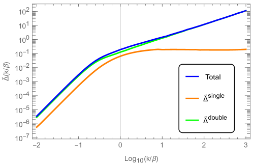
Figure 5: The calculation result of $\tilde{\Delta}(k/\beta)=N_{\rm walls}^{-1}(H_{*}/\beta)^{-1}(\beta d_{\rm DW})^{-2}\Delta(k/\beta)$. The blue line is the sum of orange (single expanding string-loop contribution, Eq. (3.84)) and green (two expanding string-loop contribution, Eq. (3.62)) lines.

The result of calculation is shown in Fig. 5. One can see that the result exhibits asymptotic power laws,

$$\Delta^{\mathrm{}}(k/\beta)\propto\begin{cases}k^{3}&(k/\beta\ll 1)\\ k&(k/\beta\gg 1)\end{cases}\,.$$ (3.88)

In addition, $\Delta^{\mathrm{}}(k/\beta)$ can be fitted by following function

$$\Delta^{\mathrm{}}(k/\beta)\simeq N_{\rm walls}\,\frac{H_{*}}{\beta}\,(\beta d_{\rm DW})^{2}\frac{a}{\left[\left(k/\beta\right)^{-3/c}+b\left(k/\beta\right)^{-1/c}\right]^{c}},$$ (3.89)

with $a\simeq 2.75302$, $b\simeq 482.381$, and $c\simeq 0.51702$. Note that one must put a UV cutoff for $k$, $k\sim\mathrm{min}\left(d_{\rm DW}^{-1},R_{c}^{-1}\right)$ (see Sec. 5), above which our calculation is not reliable. Also, $H_{*}/\beta<1$ and $\beta d_{\rm DW}<1$ work as suppression factors of the spectrum $\Delta(k/\beta)$.

The numerical plot shows that the contribution from two expanding string loops dominates the spectrum. Moreover, the dominant contribution of two expanding string loops is coming from the term proportional to $g_{a,{\rm non}}^{\prime\prime}(r,t_{d})g_{a,{\rm non}}^{\prime\prime}(r,-t_{d})$, i.e., the non overlapped region of string loops. Also, this term gives a peculiar behavior that $\Delta(k/\beta)$ linearly grows in the UV regime, which is consistent with the argument in Ref. RoperPol:2022iel since it provides a constant-source contribution in time. Intuitively, the UV regime corresponds to small string loops. Therefore, this implies that the small string loops radiate GWs even when they perfectly circular before their collisions, which is consistent with the analysis in Appendix A.

4 Present stochastic GW spectrum

We have seen so far the GW spectrum emitted from the hybrid defects of the DWs and cosmic strings. Let us here consider how it would be observed by the current GW observatories.

4.1 Production scenarios of hybrid defects

The amplitude and typical frequency of the emitted GWs depend highly on how the DWs are produced and evolved. We here present two representative scenarios; (A) scaling scenario and (B) non-thermal non-scaling scenario. In both scenarios, we assume that the pre-existing string network is diluted away by the cosmic inflation. For the scenario (A), the phase transition to produce the walls takes place either of thermal or non-thermal effects. Afterwards, due to the free random motion of the walls and their reconnection, the walls evolve into the scaling regime, in which the number of the DWs within one Hubble patch becomes of the order of unity. Eventually, the string loops are nucleated and start to expand. In this scenario, the spectrum is insensitive to the detailed way of the wall production as long as they reach the scaling regime.

For the scenario (B), on the other hand, the fields constituting the walls are decoupled from the thermal bath of the universe before the stage of the production of the walls. Thus the fields feel Hubble friction, which prevents them from rolling down in the potential. The phase transition to produce the walls takes place when the Hubble friction is balanced with the negative curvature of the potential. The typical width of the created walls can be as large as the Hubble length scale at that time while the curvature radius of the DWs depends on how the fluctuation of the field was produced; For instance, the random kick during the inflation produces scale-invariant fluctuation. Here we do not specify the curvature radius since it is beyond the scope of this paper, but assume it to be larger than $1/\beta$ for viability of our calculation as stated above. Subsequently, string loops are supposed to be nucleated well before the walls evolve into the scaling regime. In this scenario, the GW spectrum can be amplified compared to scenario (A) because of two reasons: the wall width $d_{\mathrm{DW}}$ (square of which the spectrum function $\Delta(k)$ is proportional to) can be taken closed to the Hubble length $H_{*}$ at most, and the non-scaling configuration can give large number of the walls $N_{\mathrm{walls}}$.

4.2 Redshift

The spectrum of the emitted GWs is affected by the redshift due to the Hubble expansion of the universe. The scale factor at the phase transition (string loop creation) $a_{*}$ and at the present $a_{0}$ is related by

$$\frac{a_{*}}{a_{0}}=7.97\times 10^{-16}\left(\frac{g_{*}}{100}\right)^{-\frac{1}{3}}\left(\frac{T_{*}}{100\,\mathrm{GeV}}\right)^{-1},$$ (4.1)

by using the entropy conservation during the radiation dominated era, $s_{*}a_{*}^{3}=s_{0}a_{0}^{3}$. Here, “$*$” denotes the time around when the loop creation completed and $g_{*}$ is the total number of the relativistic degrees of freedom at $T=T_{*}$. The emitted frequency $f_{*}$ and the present red-shifted frequency $f_{0}$ are related as

$$f_{0}=1.65\times 10^{-5}\ {\rm Hz}\left(\frac{f_{*}}{\beta}\right)\left(\frac{\beta}{H_{*}}\right)\left(\frac{T_{*}}{100\ {\rm GeV}}\right)\left(\frac{g_{*}}{100}\right)^{\frac{1}{6}}.$$ (4.2)

Here, $H_{*}=\sqrt{g_{*}\pi^{2}/90}\,T_{*}^{2}/M_{Pl}$ where $M_{Pl}=1/\sqrt{8\pi G}\approx 2.435\times 10^{18}$ GeV. The energy fraction of the gravitational waves at present is defined as

$$(\Omega_{\rm GW}h^{2})_{0}\equiv\frac{\rho_{\mathrm{GW,0}}}{\rho_{c}}h^{2}= 1.64\times 10^{-5}\left(\frac{g_{*}}{100}\right)^{-\frac{1}{3}}\Omega_{\rm GW*},$$ (4.3)

$$= 1.64\times 10^{-5}\left(\frac{g_{*}}{100}\right)^{-\frac{1}{3}}\kappa^{2}\left(\frac{H_{*}}{\beta}\right)^{2}\left(\frac{\alpha(t_{*})}{1+\alpha(t_{*})}\right)^{2}\Delta(k_{*}),$$ (4.4)

by using the energy conservation of the gravitational wave $(\Omega_{\rm GW}H^{2}a^{4})_{0}=(\Omega_{\rm GW}H^{2}a^{4})_{*}$, $H_{0}=2.13\times 10^{-42}h$ GeV and Eq. (3.23).

4.3 Present spectrum

Because the nucleation processes are random and their typical length scale is sufficiently small compared to the current observation scale, the signal can be regarded as stochastic and almost isotropic. Such a stochastic GW spectrum can be observed by the current and future GW observatories.

4.3.1 Scaling solution case

First, we consider the case (A), the DW became the scaling solution before the string loops are nucleated. Here we take the width of the walls as $d_{\mathrm{DW}}\sim 1/v_{\sigma}$. In this case, one should note that there is an additional contribution from the domain-wall network until the walls decay since the network continuously generates GWs to remain in the scaling regime. Such a spectrum is studied in Ref. Dunsky:2021tih and found to be of the order of

$$\left.\left(\Omega_{\mathrm{GW}}h^{2}\right)_{0}\right|_{\text{wall network}}\lesssim 10^{-4}\times\left(\frac{G\sigma}{H_{*}}\right)^{2}$$ (4.5)

at most. On the other hand, in the scaling scenario, the amplitude of the GWs calculated in Eq. (4.4) is estimated as

$$(\Omega_{\rm GW}h^{2})_{0}\lesssim 10^{-6}\,\frac{H_{*}}{v_{\sigma}}\left(\frac{\alpha(t_{*})}{1+\alpha(t_{*})}\right)^{2}\,,$$ (4.6)

which approaches

$$\begin{cases}\displaystyle 10^{-6}\,\frac{H_{*}}{v_{\sigma}}&\alpha(t_{*})\gg 1\\[8.61108pt] \displaystyle 10^{-6}\,\frac{H_{*}}{v_{\sigma}}\left(\frac{G\sigma}{H_{*}}\right)^{2}&\alpha(t_{*})\ll 1\,,\end{cases}$$ (4.7)

where we have substituted $k_{\mathrm{max}}\sim 1/d_{\mathrm{DW}}$ and have used that $\alpha(t_{*})\sim G\sigma/H_{*}$ at the scaling regime. These expressions are much smaller than Eq. (4.5) in both region $\alpha(t_{*})\gtrless 1$. Therefore, in the scenario (A), the hybrid defects do not give significant amount of the GWs, and hence the main contribution to the GW spectrum comes from the wall network, Eq. (4.5).

4.3.2 Non-thermal and non-scaling case

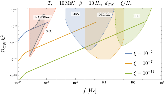
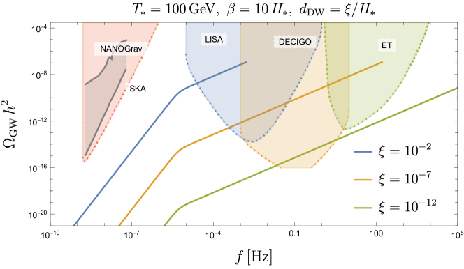
Figure 6: Present GW spectrum produced by expansion of string loops for the case of non-thermal production and non-scaling configuration of DWs. The string loops are assumed to be nucleated well before that the DWs follow the scaling regime. Each curve corresponds to different choices of $\xi$, which parameterizes the DW width (see the text). The DW VEV is taken so that $\alpha\sim 1$ for each line. The sensitivity curves of LISA, DECIGO, ET, and SKA are also shown. We also show the NANOGrav 15-yr signal as gray region. One can see that the blue curve in the upper panel can explain the NANOGrav signal. For other parameters, we expect that they will be tested by future GW observatories.

Next, we consider the case (B), that is, the walls are produced non-thermally and do never reach the scaling regime. Because the typical width of the produced walls is around the Hubble length at the production stage, we can take the width of the walls as $d_{\mathrm{DW}}\sim d_{H}|_{\text{wall production}}$, which we parameterize as $d_{\mathrm{DW}}=\xi/H_{*}$ with $\xi\leq 1$. Moreover, due to the non-scaling regime, $N_{\mathrm{walls}}$ is not necessarily $\mathcal{O}(1)$, but is taken as $N_{\mathrm{walls}}=d_{H_{*}}/d_{\mathrm{DW}}$ as the most optimistic (densest) case. If the DWs are immediately produced since the fields start to roll down in the potential and the string loops are nucleated just after the wall production, then $\xi$ would be $\mathcal{O}(1)$. Taking into account some time lag, we take some benchmark values of $\xi(<1)$. The maximum value of the amplitude of the GWs in Eq. (4.4) is estimated as

$$(\Omega_{\rm GW}h^{2})_{0}\lesssim 10^{-6}\left(\frac{H_{*}}{\beta}\right)^{2}\left(\frac{\alpha(t_{*})}{1+\alpha(t_{*})}\right)^{2}k_{*}\,d_{\mathrm{DW}}\,$$ (4.8)

from which one can expect significant amount of the GWs.

Fig. 6 shows the GW spectrum emitted from the hybrid defects with $T_{*}=10\,\mathrm{MeV}$ (top) and $T_{*}=100\,\mathrm{GeV}$ (bottom). The wall tension is taken so that the energy fraction $\alpha(t_{*})$ exceeds the order of unity, $\sigma\sim(d_{\mathrm{DW}}/d_{H_{*}})T_{*}^{2}M_{\mathrm{Pl}}$. We overlay the signal reported by the NANOGrav collaboration based on 15-year data set NANOGrav:2023gor as gray region and projected sensitivity curves of planned future observatories: DECIGO Kawamura:2020pcg (orange), Einstein Telescope (ET) Maggiore:2019uih (green), LISA Bartolo:2016ami (blue), and Square Kilometer Array (SKA) Janssen:2014dka (red). The sensitivity curves are taken from Ref. Schmitz:2020syl . Note that we put an cutoff for higher frequency region at $f_{*}=1/d_{\mathrm{DW}}$. For other possible UV cutoffs, see Sec. 5. Remarkably, the NANOGrav signal may be explained by the GW spectrum from the hybrid defects when $T_{*}=10\,\mathrm{MeV}$, $\beta=10H_{*}$, $d_{\mathrm{DW}}=10^{-2}/H_{*}$, and $\sigma\simeq(10^{4}\,\mathrm{GeV})^{3}$ (blue curve in the top panel).

Note that in this scenario (B), the domain-wall network does not emit sufficient amount of GWs because the walls are not in the scaling regime. Thus, the hybrid defects give the leading contribution.

5 Discussion and conclusion

In this paper, we analytically calculated the GW spectrum emitted from hybrid defects of DW and cosmic string, especially expanding string loops on the DWs. The derived spectrum agrees with the universal behavior $f^{3}$ ($f$: frequency) in the IR regime below $\beta$ whereas it becomes the linear behavior in the UV regime, exhibiting clear contrast to any other GW sources. This is not counter-intuitive because the expanding loops can radiate GWs even when they are perfectly circular before the collisions. Indeed, the circular-shape loop only has the $O(2)$ symmetry, which does not prevent the GW emission but has the non-zero and time-dependent quadrupole moment of the energy density. Moreover, it turned out that the pulsar timing data in the $\mathcal{O}(1-10)$ nHz frequency band recently reported by NANOGrav, EPTA, PPTA, and CPTA groups can be attributed to the predicted GW spectrum from the hybrid defects with appropriate parameters. This GW spectrum is also detectable by future GW observatories such as DECIGO, Einstein Telescope, LISA, and Square Kilometer Array.

Note that our calculation has three UV cutoffs, corresponding to the initial radius of the nucleated loops $R_{c}$, the DW width $d_{\mathrm{DW}}$, and the string width $d_{\mathrm{st}}$. In the $f_{*}\gtrsim R_{c}^{-1}$ regime, we should take into account the finite size of the nucleated loops and modify the geometric consideration of the past light cones due to the finite speed of the expanding loops. For $f_{*}\gtrsim d_{\mathrm{st}}^{-1}$, we have to take into account microscopic degrees of freedom of the strings, which may modify the spectrum in such a regime. For $f_{*}\gtrsim d_{\mathrm{DW}}^{-1}$, our thin-wall approximation breaks down. In order for the nucleated loops to expand, $R_{c}>d_{\mathrm{st}}$ is required by definition, leading to the UV cutoff $f_{*}=\mathrm{min}(d_{\mathrm{DW}}^{-1},R_{c}^{-1})$. Since we considered the non-thermal scenario for the production of the DWs in order to provide significant amount of GW, $d_{\mathrm{DW}}$ is typically the largest length scale among them, so that we put the cutoff $f_{*}=d_{\mathrm{DW}}^{-1}$ in Fig. 6.

While our result should be reliable as long as the assumptions we made are met, it is still important to check the agreement in a different way, such as field-theoretic numerical simulations. It is also important to calculate the macroscopic parameters from the field-theoretic point of view, which would be helpful in order to distinguish/exclude models of particle physics. Furthermore, the envelope approximation that we rely on through the calculation might be got rid of using a similar strategy adopted in the bubble nucleation case Jinno:2017fby , which allows us to obtain more precise result. As an application, our calculation might be applied to decaying DWs triggered by primordial black holes Stojkovic:2005zh , which can be an alternative probe for them.

Appendix A GW from circular shape loop

One may consider that the expanding uncollided string loop with the circular shape does not radiate GW due to the symmetry. However, this is not the case. Let us calculate the quadrupole of the single loop explicitly. The produced GW in the TT gauge is proportional to the second time derivative of the quadrupole $Q_{ij}$ of the energy density,

$$h_{ij}^{\mathrm{TT}} \propto(P_{ik}P_{jl}-\frac{1}{2}P_{ij}P_{kl})\ddot{Q}^{kl},$$ (A.1)

$$Q_{ij} =\int d^{3}x\,\rho^{s}(x)\left[x_{i}x_{j}-\frac{1}{3}\delta_{ij}|\vec{x}|^{2}\right],$$ (A.2)

$$P^{ij} =\delta^{ij}-\hat{n}_{\rm obs}^{i}\hat{n}_{\rm obs}^{j},$$ (A.3)

where $\rho^{s}(x)$ is given by Eq. (3.21) and $\rho^{s}(x)=0$ off the wall. Here, $\hat{n}_{\rm obs}^{i}$ represents the unit vector pointing to an observer. The DW is located on the $x-z$ plane. Assuming that the hole is nucleated at $t=0$, leading to $r_{s}(t)\simeq t$, then we get

$$Q_{ij} =d_{\mathrm{DW}}\int_{0}^{2\pi}d\phi\int_{t}^{t+\ell_{s}}drr\,\frac{\kappa\rho_{\mathrm{re}}t}{2\ell_{s}}\left[x_{i}x_{j}-\frac{1}{3}\delta_{ij}r^{2}\right]$$ (A.4)

$$=\int_{0}^{2\pi}d\phi\,\frac{\kappa\rho_{\mathrm{re}}t}{8\ell_{s}}d_{\mathrm{DW}}\left[(t+\ell_{s})^{4}-t^{4}\right]\left[\begin{pmatrix}\cos^{2}\phi&0&\cos\phi\sin\phi\\ 0&0&0\\ \cos\phi\sin\phi&0&\sin^{2}\phi\end{pmatrix}-\frac{1}{3}\delta_{ij}\right]$$ (A.5)

$$=\frac{\kappa\rho_{\mathrm{re}}}{2}d_{\mathrm{DW}}t^{4}\begin{pmatrix}\displaystyle+\frac{1}{6}&0&0\\ 0&\displaystyle-\frac{1}{3}&0\\ 0&0&\displaystyle+\frac{1}{6}\end{pmatrix}\,.$$ (A.6)

The direction of the observer is set as $\hat{n}_{\rm obs}=(\sin\theta_{\rm obs}\cos\phi_{\rm obs},\cos\theta_{\rm obs},\sin\theta_{\rm obs}\sin\phi_{\rm obs})$. The TT-projection acts on the quadrupole as

$$h^{\rm TT}_{ij}\propto \frac{\kappa\rho_{\mathrm{re}}}{2}d_{\mathrm{DW}}t^{2}\sin^{2}\theta_{\rm obs}\begin{pmatrix}\displaystyle\tilde{h}_{11}&\tilde{h}_{12}&\tilde{h}_{13}\\ \tilde{h}_{12}&\displaystyle\tilde{h}_{22}&\tilde{h}_{23}\\ \tilde{h}_{13}&\tilde{h}_{23}&\displaystyle\tilde{h}_{33}\end{pmatrix}\,,$$ (A.7)

where

$$\tilde{h}_{11}= \frac{3}{4}[1-3\cos(2\phi_{\rm obs})-2\cos(2\theta_{\rm obs})\cos^{2}\phi_{\rm obs}],$$ (A.8)

$$\tilde{h}_{12}= 3\cos\theta_{\rm obs}\sin\theta_{\rm obs}\cos\phi_{\rm obs},$$ (A.9)

$$\tilde{h}_{13}= -\frac{3}{4}\sin(2\phi_{\rm obs})[3+\cos(2\theta_{\rm obs})],$$ (A.10)

$$\tilde{h}_{22}= -3\sin^{2}\theta_{\rm obs},$$ (A.11)

$$\tilde{h}_{23}= 3\cos\theta_{\rm obs}\sin\theta_{\rm obs}\sin\phi_{\rm obs},$$ (A.12)

$$\tilde{h}_{33}= \frac{3}{4}[1+3\cos(2\phi_{\rm obs})-2\cos(2\theta_{\rm obs})\sin^{2}\phi_{\rm obs}].$$ (A.13)

Therefore, $h^{\rm TT}_{ij}\neq 0$, and hence the circular-shape loop does radiate GW.

From the expression of $Q_{ij}$, one can roughly deduce the GW spectrum $\Delta(k/\beta)$ radiated from expanding loops based on a simple model. Let us assume that all of the string loops have roughly the same radius $r_{s}(t)$. The radiated GW energy per unit time is expressed with the quadrupole as

$$\frac{dE_{\mathrm{GW}}}{dt}=\frac{G}{5}\left(\dddot{Q}_{ij}\right)^{2}\,.$$ (A.14)

Since the time scale of the decay process of the DWs is given by $\beta^{-1}$, the GW energy radiated from each loop during the process is estimated as

$$\Delta E_{\mathrm{GW}}\sim\frac{G}{\beta}\left(\kappa\rho_{re}\,d_{\mathrm{DW}}\,t\right)^{2}\,.$$ (A.15)

Summing this over multiple loops on the DW, the total GW energy is given as

$$\sum_{\text{loops}}\Delta E_{\mathrm{GW}} \sim G\sum_{a,b}\dddot{Q}_{ij}^{a}\dddot{Q}_{ij}^{b}$$ (A.16)

$$\sim G\sum_{a}\left(\dddot{Q}_{ij}^{a}\right)^{2}+G\sum_{a\neq b}\dddot{Q}_{ij}^{a}\dddot{Q}_{ij}^{b}$$ (A.17)

where $a,b$ label the string loops. In the first term, the summation gives a factor $\sim 1/(\beta r_{s}(t))^{2}$, corresponding to the number of the loops within the relevant system area $1/\beta^{2}$. In the second term, the summation gives the number of pairs of the loops that are nucleated within the time interval $r_{s}(t)$ (otherwise they cannot communicate with each other causally), which is given as

$$\frac{1}{(\beta r_{s}(t))^{4}}\beta r_{s}(t)\sim\frac{1}{(\beta r_{s}(t))^{3}}\,.$$ (A.18)

Noting $r_{s}(t)\sim t$, we get

$$\sum_{\text{loops}}\Delta E_{\mathrm{GW}}\sim\frac{G}{\beta^{3}}\left(\kappa\rho_{re}\,d_{\mathrm{DW}}\right)^{2}\left[1+\frac{1}{\beta t}\right]\,.$$ (A.19)

Translating this into the spectrum function $\Delta$ with the loop radius $r_{s}\sim t$ identified with the inverse of the frequency $1/k$, roughly we get

$$\Delta(k)\sim\frac{H_{*}}{\beta}(\beta\,d_{\mathrm{DW}})^{2}\left[1+\frac{k}{\beta}\right]$$ (A.20)

per one DW. The first term does not depend on the loop radius and agrees with the flat UV behavior of $\Delta^{\mathrm{single}}(k)$ in Eq. (3.84) and in Fig. 5 while the second term is proportional to $k$ linearly and agrees with $\Delta^{\mathrm{double}}(k)$ in the UV regime.

Appendix B (Next) Leading $k$-cancellation

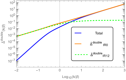
Figure 7: The spectrum $\tilde{\Delta}^{\rm double}(k/\beta)=N_{\rm walls}^{-1}(H_{*}/\beta)^{-1}(\beta d_{\rm DW})^{-2}\Delta^{\rm double}(k/\beta)$ of Eq. (3.68) (green line) and Eq. (3.76) (orange line). The blue line is the sum of Eq. (3.68) and Eq. (3.76). The positive value is shown by solid line. For the negative value, its absolute value is shown by dashed line.

Here, the numerical calculation result of Eqs. (3.68) and (3.76) is shown in Fig. 7. The result shows that the dependence of $k^{1}$ (and $k^{2}$) is canceled in small $k$ region. Similarly, the numerical calculation result of $\Delta^{\rm single}(k/\beta)$ is shown in Fig. 8. Here, the dimensionless quantity $\Delta^{\rm single}(k/\beta)$ is decomposed as

$$\Delta^{\rm single}_{0}(k/\beta)= \frac{3}{4\pi}\beta k^{3}\int_{0}^{\infty}dt_{d}\cos(kt_{d})\int_{t_{d}}^{\infty}dr\frac{C_{\rm DW}(r)}{r^{3}\mathcal{I}(r,t_{d})}j_{0}(kr)F_{0}^{\prime\prime}(r,t_{d}),$$ (B.1)

$$\Delta^{\rm single}_{1}(k/\beta)= \frac{3}{4\pi}\beta k^{3}\int_{0}^{\infty}dt_{d}\cos(kt_{d})\int_{t_{d}}^{\infty}dr\frac{C_{\rm DW}(r)}{r^{3}\mathcal{I}(r,t_{d})}\frac{j_{1}(kr)}{kr}F_{1}^{\prime\prime}(r,t_{d}),$$ (B.2)

$$\Delta^{\rm single}_{2}(k/\beta)= \frac{3}{4\pi}\beta k^{3}\int_{0}^{\infty}dt_{d}\cos(kt_{d})\int_{t_{d}}^{\infty}dr\frac{C_{\rm DW}(r)}{r^{3}\mathcal{I}(r,t_{d})}\frac{j_{2}(kr)}{(kr)^{2}}F_{2}^{\prime\prime}(r,t_{d}).$$ (B.3)

Then, the linear $k$ dependence is cancelled in large $k$ region in this case.

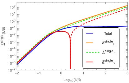
Figure 8: The quantity $\tilde{\Delta}^{\rm single}(k/\beta)=N_{\rm walls}^{-1}(H_{*}/\beta)^{-1}(\beta d_{\rm DW})^{-2}\Delta^{\rm single}(k/\beta)$ is calculated by summing up each $j_{i}(kr)$ component (blue line). The positive value is shown by solid line. The negative value is taken its absolute value and shown by dashed line. The sign of $\Delta^{\rm single}_{2}(k/\beta)$ is positive for $\log_{10}(k/\beta)\lesssim 0.4$ and negative for $\log_{10}(k/\beta)\gtrsim 0.4$. The linear $k$ dependence of $\Delta^{\rm single}_{i}(k/\beta)$ is canceled by summing up.

References

- (1) LIGO Scientific, Virgo collaboration, Observation of Gravitational Waves from a Binary Black Hole Merger, Phys. Rev. Lett. 116 (2016) 061102 [1602.03837].
- (2) LIGO Scientific, Virgo collaboration, GW150914: The Advanced LIGO Detectors in the Era of First Discoveries, Phys. Rev. Lett. 116 (2016) 131103 [1602.03838].
- (3) LIGO Scientific, Virgo collaboration, GW150914: First results from the search for binary black hole coalescence with Advanced LIGO, Phys. Rev. D 93 (2016) 122003 [1602.03839].
- (4) LIGO Scientific, Virgo collaboration, Properties of the Binary Black Hole Merger GW150914, Phys. Rev. Lett. 116 (2016) 241102 [1602.03840].
- (5) LIGO Scientific, Virgo collaboration, GW170817: Observation of Gravitational Waves from a Binary Neutron Star Inspiral, Phys. Rev. Lett. 119 (2017) 161101 [1710.05832].
- (6) A. Kosowsky, M. S. Turner and R. Watkins, Gravitational radiation from colliding vacuum bubbles, Phys. Rev. D 45 (1992) 4514.
- (7) A. Kosowsky and M. S. Turner, Gravitational radiation from colliding vacuum bubbles: envelope approximation to many bubble collisions, Phys. Rev. D 47 (1993) 4372 [astro-ph/9211004].
- (8) M. Kamionkowski, A. Kosowsky and M. S. Turner, Gravitational radiation from first order phase transitions, Phys. Rev. D 49 (1994) 2837 [astro-ph/9310044].
- (9) C. Grojean and G. Servant, Gravitational Waves from Phase Transitions at the Electroweak Scale and Beyond, Phys. Rev. D 75 (2007) 043507 [hep-ph/0607107].
- (10) C. Caprini, R. Durrer, T. Konstandin and G. Servant, General Properties of the Gravitational Wave Spectrum from Phase Transitions, Phys. Rev. D 79 (2009) 083519 [0901.1661].
- (11) C. Caprini et al., Science with the space-based interferometer eLISA. II: Gravitational waves from cosmological phase transitions, JCAP 04 (2016) 001 [1512.06239].
- (12) C. Caprini and D. G. Figueroa, Cosmological Backgrounds of Gravitational Waves, Class. Quant. Grav. 35 (2018) 163001 [1801.04268].
- (13) C. Caprini et al., Detecting gravitational waves from cosmological phase transitions with LISA: an update, JCAP 03 (2020) 024 [1910.13125].
- (14) P. Athron, C. Balázs, A. Fowlie, L. Morris and L. Wu, Cosmological phase transitions: From perturbative particle physics to gravitational waves, Prog. Part. Nucl. Phys. 135 (2024) 104094 [2305.02357].
- (15) A. Vilenkin, Gravitational radiation from cosmic strings, Phys. Lett. B 107 (1981) 47.
- (16) F. S. Accetta and L. M. Krauss, The stochastic gravitational wave spectrum resulting from cosmic string evolution, Nucl. Phys. B 319 (1989) 747.
- (17) R. R. Caldwell and B. Allen, Cosmological constraints on cosmic string gravitational radiation, Phys. Rev. D 45 (1992) 3447.
- (18) A. Vilenkin and E. S. Shellard, Cosmic Strings and Other Topological Defects. Cambridge University Press, 7, 2000.
- (19) T. W. B. Kibble, G. Lazarides and Q. Shafi, Walls Bounded by Strings, Phys. Rev. D 26 (1982) 435.
- (20) A. Vilenkin and A. E. Everett, Cosmic Strings and Domain Walls in Models with Goldstone and PseudoGoldstone Bosons, Phys. Rev. Lett. 48 (1982) 1867.
- (21) A. E. Everett and A. Vilenkin, Left-right Symmetric Theories and Vacuum Domain Walls and Strings, Nucl. Phys. B 207 (1982) 43.
- (22) J. Preskill and A. Vilenkin, Decay of metastable topological defects, Phys. Rev. D 47 (1993) 2324 [hep-ph/9209210].
- (23) M. Kawasaki and K. Nakayama, Axions: Theory and Cosmological Role, Ann. Rev. Nucl. Part. Sci. 63 (2013) 69 [1301.1123].
- (24) M. Eto, Y. Hamada and M. Nitta, Composite topological solitons consisting of domain walls, strings, and monopoles in O(N) models, JHEP 08 (2023) 150 [2304.14143].
- (25) D. I. Dunsky, A. Ghoshal, H. Murayama, Y. Sakakihara and G. White, GUTs, hybrid topological defects, and gravitational waves, Phys. Rev. D 106 (2022) 075030 [2111.08750].
- (26) M. Gleiser and R. Roberts, Gravitational waves from collapsing vacuum domains, Phys. Rev. Lett. 81 (1998) 5497 [astro-ph/9807260].
- (27) J. Preskill, S. P. Trivedi, F. Wilczek and M. B. Wise, Cosmology and broken discrete symmetry, Nucl. Phys. B 363 (1991) 207.
- (28) T. Hiramatsu, M. Kawasaki and K. Saikawa, On the estimation of gravitational wave spectrum from cosmic domain walls, JCAP 02 (2014) 031 [1309.5001].
- (29) K. Saikawa, A review of gravitational waves from cosmic domain walls, Universe 3 (2017) 40 [1703.02576].
- (30) N. Kitajima, J. Lee, K. Murai, F. Takahashi and W. Yin, Gravitational waves from domain wall collapse, and application to nanohertz signals with QCD-coupled axions, Phys. Lett. B 851 (2024) 138586 [2306.17146].
- (31) R. Jinno and M. Takimoto, Gravitational waves from bubble collisions: An analytic derivation, Phys. Rev. D 95 (2017) 024009 [1605.01403].
- (32) R. Jinno and M. Takimoto, Gravitational waves from bubble dynamics: Beyond the Envelope, JCAP 01 (2019) 060 [1707.03111].
- (33) S. Blasi, R. Jinno, T. Konstandin, H. Rubira and I. Stomberg, Gravitational waves from defect-driven phase transitions: domain walls, JCAP 10 (2023) 051 [2302.06952].
- (34) S. Blasi and A. Mariotti, QCD Axion Strings or Seeds?, 2405.08060.
- (35) NANOGrav collaboration, The NANOGrav 15 yr Data Set: Evidence for a Gravitational-wave Background, Astrophys. J. Lett. 951 (2023) L8 [2306.16213].
- (36) EPTA, InPTA: collaboration, The second data release from the European Pulsar Timing Array - III. Search for gravitational wave signals, Astron. Astrophys. 678 (2023) A50 [2306.16214].
- (37) H. Xu et al., Searching for the Nano-Hertz Stochastic Gravitational Wave Background with the Chinese Pulsar Timing Array Data Release I, Res. Astron. Astrophys. 23 (2023) 075024 [2306.16216].
- (38) D. J. Reardon et al., Search for an Isotropic Gravitational-wave Background with the Parkes Pulsar Timing Array, Astrophys. J. Lett. 951 (2023) L6 [2306.16215].
- (39) M. Hindmarsh and T. W. B. Kibble, Monopoles on strings, Phys. Rev. Lett. 55 (1985) 2398.
- (40) C. Caprini, R. Durrer and G. Servant, Gravitational wave generation from bubble collisions in first-order phase transitions: An analytic approach, Phys. Rev. D 77 (2008) 124015 [0711.2593].
- (41) A. Roper Pol, C. Caprini, A. Neronov and D. Semikoz, Gravitational wave signal from primordial magnetic fields in the Pulsar Timing Array frequency band, Phys. Rev. D 105 (2022) 123502 [2201.05630].
- (42) S. Kawamura et al., Current status of space gravitational wave antenna DECIGO and B-DECIGO, PTEP 2021 (2021) 05A105 [2006.13545].
- (43) M. Maggiore et al., Science Case for the Einstein Telescope, JCAP 03 (2020) 050 [1912.02622].
- (44) N. Bartolo et al., Science with the space-based interferometer LISA. IV: Probing inflation with gravitational waves, JCAP 12 (2016) 026 [1610.06481].
- (45) G. Janssen et al., Gravitational wave astronomy with the SKA, PoS AASKA14 (2015) 037 [1501.00127].
- (46) K. Schmitz, New Sensitivity Curves for Gravitational-Wave Signals from Cosmological Phase Transitions, JHEP 01 (2021) 097 [2002.04615].
- (47) D. Stojkovic, K. Freese and G. D. Starkman, Holes in the walls: Primordial black holes as a solution to the cosmological domain wall problem, Phys. Rev. D 72 (2005) 045012 [hep-ph/0505026].