Constraining gravity by Pulsar SAX J1748.9-2021 observations
Abstract
We discuss spherically symmetric dynamical systems in the framework of a general model of gravity, i.e. , where is a dimensional quantity in squared length units [L2]. We initially assume that the internal structure of such systems is governed by the Krori-Barua ansatz, alongside the presence of fluid anisotropy. By employing astrophysical observations obtained from the pulsar SAX J1748.9-2021, derived from bursting X-ray binaries located within globular clusters, we determine that is approximately equal to km2. In particular, the model can create a stable configuration for SAX J1748.9-2021, encompassing its geometric and physical characteristics. In gravity, the Krori-Barua approach links and , which represent the components of the pressures, to (), representing the density, semi-analytically. These relations are described as and . Here, the expression and represent the radial and tangential sound speeds, respectively. Meanwhile, pertains to the surface density and is derived using the parameters of the model. Notably, within the frame of gravity where is negative, the maximum compactness, denoted as , is inherently limited to values that do not exceed the Buchdahl limit. This contrasts with general relativity or with with positive , where has the potential to reach the limit of the black hole asymptotically. The predictions of such model suggest a central energy density which largely exceeds the saturation of nuclear density, which has the value g/cm3. Also, the density at the surface surpasses . We obtain the relation between mass and radius represent it graphically, and show that it is consistent with other observational data.
I Introduction
Experiments measuring the perihelion advance of Mercury, the gravitational Doppler effect, and light deflection, all of which are used to evaluate the accuracy of Einstein’s general relativity (GR) at solar-system scales, have demonstrated exceptionally high precision, as reported in Will (2014). Additionally, GR has undergone tests in extreme gravitational conditions: For example, detecting gravitational waves produced by the collision of compact celestial objects Abbott et al. (2018, 2019). As a consequence, GR has risen as the most successful and widely accepted theory for explaining gravitational phenomena. However, Einstein’s theory presents shortcomings at UV scales for the lack of a viable quantum gravity, and at IR scales because significant issues related to observed Universe remain unanswered. In fact, to account for cosmic acceleration within the framework of GR, we need to introduce dark energy, which is an unusual form of matter-energy characterized by a substantial negative pressure. Furthermore, a huge amount of dark matter is required to address dynamics of cosmic structures like galaxies and clusters of galaxies. In both cases, at the moment, there is no answer at fundamental level explaining such a dark side.
In recent decades, numerous alternative gravitational theories have arisen, aiming to explain the expansion that accelerates Universe and cosmic structure dynamics. Specifically, GR can be modified or extended at UV and IR scales in order to achieve a comprehensive explanation of the early inflationary era involving dark energy, at late epochs. citeStarobinsky:1980te, Capozziello:2002rd, Carroll:2003wy, Hu:2007nk, Nojiri:2006ri, Amendola:2006we, Appleby:2007vb, Odintsov:2020nwm, Koyama:2015vza,Nojiri:2003ft, Nojiri:2007cq, Cognola:2007zu, Oikonomou:2020qah, Oikonomou:2020oex.
A straightforward method for improving GR is substituting the scalar curvature with , giving rise to what is known as gravity. Related models have been explored as potential explanations for dynamics of both early and late Universe. Comprehensive reviews on this topic are Sotiriou and Faraoni (2010); De Felice and Tsujikawa (2010); Capozziello and De Laurentis (2011); Nojiri and Odintsov (2011); Clifton et al. (2012); Nojiri et al. (2017). Conversely, at astrophysical scales, modifications of GR impact also the characteristics of compact stars. In fact, in the context of gravity, commonly known as the Starobinsky model Starobinsky (1980), and using a non-perturbative methodology, there is a significant increase in the maximum mass of compact stars on the diagram of mass and radius, primarily attributable to the quadratic term Yazadjiev et al. (2014); Astashenok et al. (2015); Yazadjiev and Doneva (2015a); Sbisà et al. (2020); Astashenok et al. (2020); Astashenok et al. (2021a, b); Nobleson et al. (2022); Jiménez et al. (2022). Researches indicate that in the context of -squared gravity, the secondary component of the GW190814 event, as reported by the LIGO-Virgo collaboration in Abbott et al. (2020), can be effectively characterized as a NS Astashenok et al. (2020); Astashenok et al. (2021a); Nashed and Saridakis (2020); Astashenok et al. (2021b). In particular, the physical properties of neutron stars (NSs) have been examined both for non-rotating Astashenok and Odintsov (2020a) and rotating Astashenok and Odintsov (2020b) systems, within the context of gravity coupled with an axion scalar field. In Olmo et al. (2020) thoroughly review stellar structure models within modified gravity theories, and develop in metric and metric-affine approaches.
It has been shown in Ref. Boehmer et al. (2008) that the flat rotation curves of galaxies can be explained by only small departures from GR. Specifically, they found that a gravitational Lagrangian taking the form represents a relatively natural modification of Einstein gravity, with the dimensionless parameter being communicated in terms of the tangential speed. In addition, there has been interest in this power-law model lately as a potential solution to the clustered galactic dark matter issue Sharma et al. (2021), where the parameter is constrained to be of the order of . In this context, Ref. Sharma et al. (2021) was used to calculate the light deflection angle using the rotational velocity profile of typical nearby galaxies in the gravitational background of . Additional investigations of the consequences of power law can be found in. Capozziello et al. (2006); Nashed (2018); Capozziello et al. (2007); Martins and Salucci (2007); Nashed and Nojiri (2020); Jaryal and Chatterjee (2021); Sharma and Verma (2022).
Conversely, it has been demonstrated that the parameter , in the context of theory, possesses a substantial influence on the mass and radius plots of isotropic NSs Astashenok et al. (2020); Capozziello et al. (2016).Although isotropic perfect fluids are commonly used to describe the matter inside compact stars, there are good reasons to take anisotropies in extremely dense matter into consideration Chaichian et al. (2000); Ferrer et al. (2010); Horvat et al. (2011); Doneva and Yazadjiev (2012); Silva et al. (2015); Yagi and Yunes (2015); Ivanov (2017); Isayev (2017); Biswas and Bose (2019); Maurya et al. (2019); Pretel (2020); Rahmansyah et al. (2020); Das et al. (2021a, b); Deb et al. (2021); Rahmansyah and Sulaksono (2021); Bordbar and Karami (2022). These studies demonstrate that the existence of anisotropy can either raise or decrease the maximal-mass threshold, thereby offering the potential to attain more massive compact stars that align with astronomical observations.
Folomeev conducted a comprehensive investigation of the impact of anisotropies on the internal structure of NSs, employing a completely autonomous non-perturbative method inside the Starobinsky mode. This study considered three distinct types of realistic equations of state (EoSs) Folomeev (2018). The incorporation of anisotropic pressure has been shown to facilitate the utilization of stiffer equations of state (EoSs) to represent configurations that meet observational criteria effectively. Furthermore, Ref.Panotopoulos et al. (2021) delved into the exploration of anisotropic quark stars within -squared gravity, and more recently, in Nashed et al. (2021) examined anisotropic compact stars in relation to theories of higher-order curvature such as .According to Farasat Shamir and Malik (2019); Nashed and El Hanafy (2023); Malik (2022); Malik et al. (2022b), a study of compact anisotropic structures in the Starobinsky form and within generalised modified gravity has been conducted. The gravitational collapse of an anisotropic system with heat flow was investigated in Ref. Usman and Shamir (2022) using the Karmarkar condition and taking a logarithmic modification of the standard Starobinsky model into account. For a comparative analysis of self-consistent charged anisotropic spheres in an embedded spacetime framework with the Karmarkar condition applied, see Ref. Ahmad et al. (2021).
To the best of our information, there is no investigation into anisotropic compact stars within the framework of the gravity model. As we will see below, this model is particularly suitable to investigate small deviations with respect to GR. With this objective at the forefront, we aim to formulate the equations that govern the stellar structure in this gravitational model and explore the impact of compact star anisotropy. For this goal,We’ll make use of the so-called Krori-Barua (KB) ansatz to close the system of differential equations.
The structure of the paper is the following: In Section II, we offer a concise overview of theory. In Section III, we introduce the specific model, namely , and derive the form of the system of differential equations, which is presented in detail in the Supplementary Material. For the sake of computational convenience, we employ the KB ansatz and deduce the expressions for density, radial pressure, and tangential pressure, as detailed in the Supplementary Material. Utilizing matching conditions, we determine the model parameters.
In Section IV, pulsar’s mass and radius from astrophysical observations of SAX J1748.9-2021 are used to derive constraints on the model parameter . In Section V,e examine the physical quantity deviations from GR and provide numerical results. Finally, in Section VI, we summarize our results. It is worth noticing that we use geometrical units and the spacetime signature for our computations. However, final results are reported in physical units.
II The Theoretical framework
II.1 gravity in metric formalism
In this section, we provide a concise overview of gravity adopting the metric formalism. The action is
| (1) |
In this study, the Ricci scalar in this case is denoted by , the matter action is denoted by , and the determinant of is . The equation of motion is obtained as follows when we change the action with respect to the metric:
| (2) |
The gravitational coupling is , with the Newton constant and the speed of light. Additionally, we have the matter energy-momentum tensor denoted as .
Furthermore, we define as the derivative of with respect to , and the covariant derivative connected to the metric’s Levi-Civita connection. Here is the d’Alembert operator. Finally, is the Ricci tensor.
In GR, for a stellar fluid is defined by its energy density and pressure, which are , where . However, in gravity, both the metric tensor and the Ricci scalar are non-trivial. Consequently, is now prescribed by a second order differential equation which can be derived from Eq. (2) as:
| (3) |
which means that in comparison to GR, where leads to , if nonlinear functions of are taken into account, additional curvature components must also be taken into consideration even when standard matter is absent. In other words, a curvature fluid has to be taken into account Capozziello (2002); Capozziello and De Laurentis (2011).
II.2 Spherical symmetry
To investigate the internal composition of a stellar in an equilibrium, we analyze a spherically symmetric system where the spacetime is characterized by the metric
| (4) |
where the spacetime is given by Schwarzschild-like coordinates . Here, and are function of only. We assume that the distribution of stellar matter is an anisotropic perfect fluid, i.e., it can be prescribed by:
| (5) |
where is the four-velocity of the fluid with the normalization condition ; is a unit radial four-vector satisfying the condition . Here, the energy density is represented by , the tangential pressure by , the radial pressure by , and the anisotropy factor by .
According to the above metric, we can express as , and as . As a result, the energy-momentum tensor (5) trace has the following form:
| (6) |
The conservation law of momentum and energy can be obtained from the divergence of Equation (5) which yields:
| (7) |
Here ′ denotes the derivative W.r.t.. Furthermore, it is
| (8) |
Hence, the energy-momentum tensor (5) and the line element (4) provide, from the field equations (2), the following non-zero components:
| (9) |
| (10) |
| (11) |
The equation governing the evolution of scalar curvature (3) now becomes
| (12) |
III The gravity model
Let us now adopt the following model:
| (13) |
where represents a parameter with dimensions [L2], with a length. When the dimensional parameter is set to zero, the standard Einstein GR is recovered. Conversely, for small non-zero , the expression can be recast as
| (14) |
For these reasons, Eq. (13) is a general model capable of representing both small and large deviations with respect to GR.
Upon inserting the expression for as provided in Eq. (13) into Eqs. (9) through (11), we derive a lengthy system, which is reported in the Supplementary Material. One can readily observe that when considering , the matter density and pressure components undergo modifications and ultimately converge to the GR solution, as demonstrated in previous works Nashed and Capozziello (2020); Roupas and Nashed (2020). Nevertheless, the system in Eqs. ( 1), ( 2), and ( 3), presented in the Supplementary Material, encompasses five unknown functions necessitating the imposition of two extra constraints to define it. A possible approach is assuming suitable EoS to establish connections between radial and tangential pressures and density. However, this approach may not be practical due to the presence of a challenging fourth-order differential equation within the system.
An alternative approach is considering reasonable assumptions for the metric potentials and . We will adopt this method and consider the so called Krori-Barua (KB) spacetime to investigate stellar models in the frame of theory of gravity.
III.1 The Krori-Barua framework
Let us introduce the metric potentials of the KB form, as described in Krori and Barua (1975):
| (15) |
here, represents the radius of the star, and the parameters are dimensionless and can be determined by satisfying junction conditions. Equation (15) ensures a singularity-free solution across the whole interior of the star. The ansatz of KB has been applied in diverse gravitational theories, including GR. However, in the present investigation, we employ observational constraints derived from the pulsar SAX J1748.9-2021 to estimate the model parameter . By employing Eq. (15) and Eqs. ( 1), ( 2), and ( 3) presented in the Supplementary Material, we can expressed the components of the energy-momentum tensor.
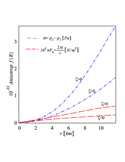
Moreover, we present the notion of the anisotropic which is defined as , which arises due to the pressure difference, equivalently represented by anisotropy . Significantly, the anisotropy becomes zero at the central point. In the strong anisotropy situation, , for , it necessitates that across the star’s interior. Conversely, in mild anisotropy case, i.e., , it requires that throughout the interior of the star.
III.2 Matching Conditions
For a stellar system, we can suppose that the vacuum solutions of GR correspond to those of given in Eq. (13). This means that the external solution simply aligns with Schwarzschild spacetime. Thus, we choose to represent vacuum space as:
| (16) |
In this context, describes star’s mass. Applying the junction conditions we get:
| (17) |
with represents compactness described as:
| (18) |
By adopting Eq. (15) and using from Eqs. (4) in the Supplementary Material, we can establish the specified surface limits. This allows us to express the model parameters in terms of and .The pulsar mass and radius can be constrained by astrophysical observations, which, in turn, determine the compactness; consequently, the next step is observationally constraining the parameter .
IV Constraints and stability considerations from SAX J1748.9-2021 observations
In this section, we utilize observational limitations, with a specific focus on and of stellar SAX J1748.9-2021, to determine the value of the parameter in the frame of theory of gravity. Furthermore, we subject the obtained solution to a thorough evaluation of its stability based on different physical limits. As mentioned earlier in the Introduction, accurate observational data plays a vital role in limiting the parameter space. To begin, our selection criteria are presented for the pulsar SAX J1748.9-2021 aiming to limit theory of gravity. This choice is based on the availability of time-resolved spectroscopic data from EXO 1745-248 during thermonuclear bursts, which has yielded precise measurements for the pulsar () and ( km) (Özel et al., 2009). By leveraging and of the pulsar SAX J1748.9-2021, we narrow of model. This parameter space comprises the set of parameters [, , , ].
IV.1 The material component
Referring to equations presented in the Supplementary Material, and taking into account numerical estimation for the model parameters, we generate plots illustrating , and as functions dependent on . These plots are reported in Figures 10(a)–0(c). The density and pressure profiles clearly adhere to the stability criteria within the material sector, which we are going to discuss below. They reach their maximum values at the core, maintain positivity, and are free of singularities throughout the star’s interior. They exhibit a monotonic decrease towards the star surface. Furthermore, we generate a figure representing the difference between pressures (i.e., anisotropy), as illustrated in plot 10(d). Such graph demonstrates that adheres the requirement of stability, as it reaches zero at the core and steadily grows in a monotonic way towards the star surface. It’s important to note that the strong anisotropy criteria, as analyzed in this study, introduces an extra positive force, proportional to , which impacts the material’s overall performance and influences hydrodynamic equilibrium. Such force acts against the force of gravity, playing a pivotal role in adjusting the size of the star, which enables it to support a larger mass compared to scenarios with isotropy or mild anisotropy. A more thorough explanation of this impact can be found in Subsection IV.7.
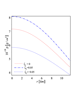
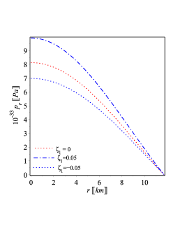
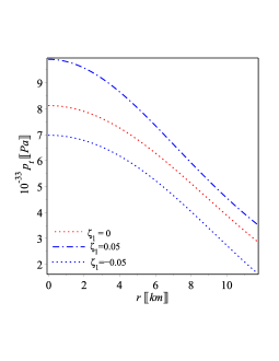
It is worth providing numerical values for physical quantities associated with the pulsar SAX J1748.9-2021, as predicted by the current model.
For instance, with , the core density is approximately g/cm3, that roughly 3 times , and both and , are approximately dyn/cm2. At the star boundary, we show g/cm3, that times g/cm3, dyn/cm2, and dyn/cm2.
When , g/cm3, that 2.16 times g/cm3, and pressure components at the center are approximately dyn/cm2. At boundary, we get g/cm3, that times g/cm3, dyn/cm2, dyn/cm2.
In this context, it is noteworthy that the stellar model under consideration doesn’t eliminate the chance that the pulsar SAX J1748.9-2021 has a core composed by neutrons. As indicated in Section III, the KB ansatz (15) has been employed as an alternative to EoSs in order to close the system presented in the Supplementary Material. Furthermore, we demonstrate that the KB efficiently establishes relations between the components of the energy-momentum tensor. In order to realize this, we present and subsequently expand the power series of Eqs. ( 4) presented in the Supplementary Material up to . It is evident that the procedure leads to the following relations:
| (19) |
The constants denoted as are entirely determined in the model parameter space, which is , as detailed in the Supplementary Material. Remarkably, we can express the equations above in a more physically meaningful way as follows:
| (20) |
In this context, we can interpret the following physical parameters as follows: represents the sound of speed in the direction, is the density (specifically, the surface density satisfying the boundary condition ), denotes the speed of sound in the tangential direction, and represents another density. It is worth noticing that the condition applies to , but not necessarily to , since may not vanish on the surface. These parameters encompass two special cases: For hadron matter, the equation of state (EoS), which is maximally compact, where =, and the EoS based on the MIT which represents the bag model of quark matter, where =. For instance, when , using Eqs. ( 4) as detailed in the Supplementary Material, we obtain the following values: , , g/cm3, and g/cm3. Likewise, for , we obtain the following values: , , g/cm3, and g/cm3.
IV.2 The geometric component
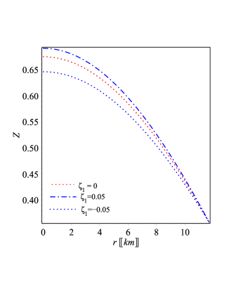
The function of the gravitational redshift, corresponding to our ansatz is as follows:
| (21) |
We creat a figure of the pulsar’s SAX J1748.9-2021 redshift function as reported in Fig. 21(a). In the GR case, i.e., , at the core is approximately , and at the boundary . If , at yields less than GR. Importantly, this value remains below the maximum limit , as discussed in (Buchdahl, 1959a; Ivanov, 2002; Barraco et al., 2003; Böhmer and Harko, 2006). Likewise, for , we observe that the upper limit of at the center is which remains below the maximum limit.
It effectively conveys that the redshift distributions in the frame of satisfy stability limits in both cases discussed. It effectively communicates that the value of and has a finite value within the star’s interior, decreasing monotonically towards the boundary, and has a positive redshift and its first derivative is negative as demonstrated in Fig. 21(a).
IV.3 Limits on the mass radius relation from SAX J1748.9-2021 observations
In the following analysis, we utilize the value of mass and the value of radius evaluated from observation of the stellar SAX J1748.9-2021, which are reported as and km according to (Özel et al., 2009), to impose constraints on the parameter within the framework of theory.
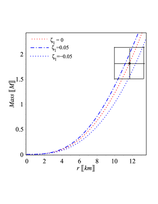
Mass distribution, within the radius of the stellar is given as:
| (22) |
Recalling the density profile presented in the Supplementary Material, for the , we show in the Fig. 21(b) that:
-
•
When , for km and . This determines the constant parameters to be [, , , , ].
-
•
For , for km and . This determines the constant parameters ro be [, , , , ].
-
•
For , the constant parameters are [, , ].
This imposes limits on km2. Generally, as represented in Fig. 21(b), the inclusion of gravity results in variations in the stellar mass. In the analysis that follows, we’ll utilize the specified numerical values to evaluate how robust current stellar is under different stability conditions.
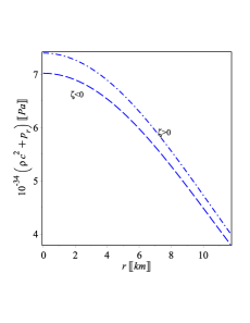
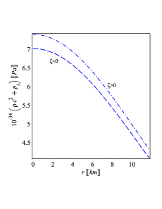
IV.4 The Zeldovich condition
An important criterion to confirm the pulsar’s stability is provided by the study of Zeldovich (Zeldovich and Novikov, 1971). According to this criterion, will never be higher than the core energy density, which means that,
| (23) |
Referring back to Eqs. ( 4) as detailed in the Supplementary Material, we can derive and as:
| (24) |
Utilizing the previous numerical values for the pulsar SAX J1748.9-2021, as discussed in Subsection IV.3, we can assess the Zeldovich inequality (23). For , the inequality becomes , which is less than 1. Similarly, for , the inequality reads , also less than 1. This ensures the validation of the condition of Zeldovich.
IV.5 The conditions of energy
It is advantageous to express Eqs. (2) as:
| (25) |
In this context, we use the notation to represent the Einstein tensor, which accounts for the correction arising from gravity De Felice and Tsujikawa (2010); Capozziello and De Laurentis (2011) as:
| (26) |
The energy-momentum tensor can be written as .
The focusing theorem and the Raychaudhuri equation imply the following inequalities for the tidal tensor: and , where signifies an arbitrary future-directed null vector and represents an arbitrary timelike vector. It is worth noticing that, within theory, the could be expressed as , as can be inferred from Eq. (25). With this consideration in mind, the energy conditions (ECs) can be extended to gravity in the following way Capozziello et al. (2015):
-
1.
, , and , which corresponds to the Weak Energy Condition (WEC).
-
2.
, and , which corresponds to the Null Energy Condition (NEC).
-
3.
, , , which corresponds to the Strong Energy Condition (SEC).
-
4.
, , , which corresponds to the Dominant Energy Conditions (DEC).
Figure 3 provides a visual representation of the ECs when . These figures confirm that the current model of pulsar SAX J1748.9-2021 verifies all the conditions listed above.
IV.6 Causality conditions
The condition of causality is consider as one of the fundamental aspects which states that the sound speed should not exceed the light speed. Referring to Eqs. (20), and can be fixed as:
| (27) |
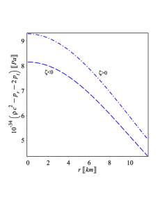
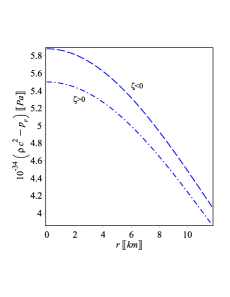
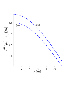
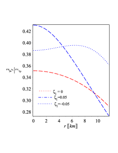
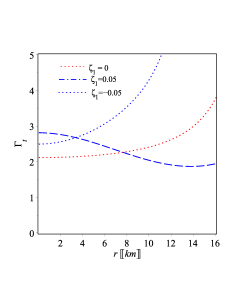
Utilizing Eqs. ( 4) in the Supplementary Material, we can determine the gradients of density and pressure components, as provided by Eqs. ( 7) in the Supplementary Material. We represent and of pulsar SAX J1748.9-2021 when , as in Figs. 43(a) and 3(b). These figures show and , satisfying the causality and stability conditions. Moreover, Fig. 43(c), illustrates that throughout the interior of pulsar SAX J1748.9-2021 (Herrera, 1992).
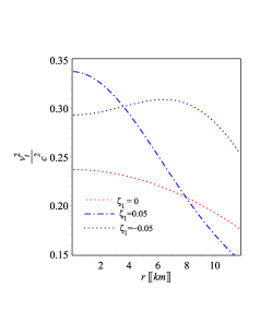
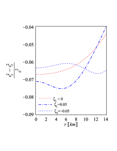
It is important to notice that the sound speed exhibits variations with , as reported in Figs. 43(a) and 3(b). Specifically, when , we observe and . Conversely, for , the intervals are and . The maximum limits correspond to speed sound at , align perfectly the values derived in IV.1 from the induced EoSs (20), specifically () and ().
IV.7 The adiabatic and the equilibrium of hydrodynamic forces
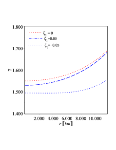
In Newtonian gravity, it’s widely accepted that there is no maximum limit on the mass of a stable configuration when the adiabatic index for a specific EoS increases . Conversely, within Newtonian gravity, it is necessary for a stable configuration that . Nevertheless, it has been shown that a star can withstand radial perturbations in a fully relativistic anisotropic neutron star model, even when . To account for this, we define the adiabatic index (Chandrasekhar, 1964; Chan et al., 1993) as follows:
| (28) |
Obviously, in the case of isotropy (), we obtain . In the mildly anisotropic case (), which is similar to the Newtonian theory, we have , consistent with the standard stability requirement. On the other hand, when strong anisotropy is involved (), similar to what is considered in this study, we find Chan et al. (1993); Heintzmann and Hillebrandt (1975).
By utilizing the field equations and Eqs. ( 4), and the gradients given by Eq. ( 7) presented in the Supplementary Material, we demonstrate that our gravity offers a stable anisotropic model for the pulsar SAX J1748.9-2021 when , as illustrated in Figure 5.”
Next, we examine the hydrodynamic equilibrium of the current model using the Tolman-Oppenheimer-Volkoff (TOV) equation, which is defined as follows:
| (29) |
Here , , and represent the typical gravitational, hydrostatic, and anisotropic forces, respectively, in additional to the force of originating from the component. These forces defined as:
| (30) |
Within the formula for the gravitational force, denoted as , we have introduced the quantity , in addition to which denotes the gravitational mass of a system that is isolated within the 3-space volume (at constant time ). This can be described by the Tolman mass formula within the framework of gravity. gravity, as described by Tolman in his 1930 work (Tolman, 1930).
| (31) | |||||
Consequently, the gravitational force can be expressed as . Utilizing the field equations ( 4) together with the gradients ( 7) in the Supplementary Material, we can demonstrate that gravity complies with (29), giving a stable model for the pulsar SAX J1748.9-2021 when , including (), as shown in Fig. 6.
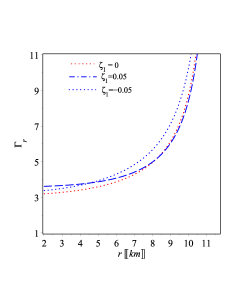
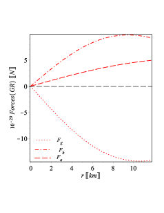
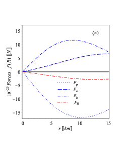
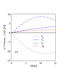
Note that () introduces positive extra force which counters the field of gravity. This is an important to enlarge the star’s size. As evident Figs. 65(b) and 65(c) demonstrate such phenomena with the additional force creating from theory when . This investigation aligns with the previously obtained results for the star SAX J1748.9-2021 in Subsection IV.3, which yielded () and ().
V Mass-radius relation and equation of state
It is worth noticing that our study refrains from imposing specific EoS assumptions; rather, we use the ansatz of KB as outlined in Eqs. (15). Nevertheless, the resulting EoSs in Eqs.(20) show how pressures and density are related in this ansatz, and they are mainly valid at the core because of the power series assumptions that underlie it. By creating a range of density and pressure values that span from the core to the surface and take taking into account the model parameter’s , we confirm the accuracy of these equations. . We construct these sequences, as shown in Fig.7., using the numerical values given in Section IV.3 for the pulsar SAX J1748.9-2021 and the equation of motions of theory of gravity, which are specifically described in Eqs. ( 4), given in the Supplementary Material.
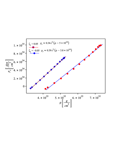
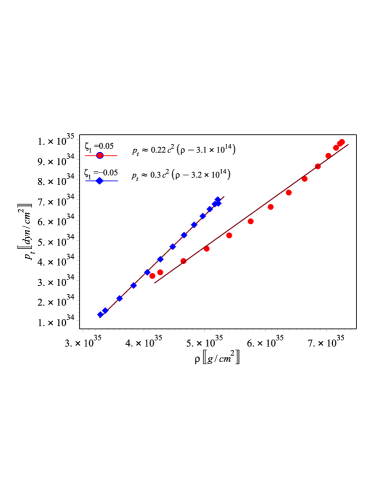
It is noteworthy that the linear best fit, in the both cases of positive/negative of , induces slight alterations in the surface density and sound speeds. Consequently, we suggest that a higher polynomial, namely , could offer a more accurate fit, yielding non-linear equations of state.
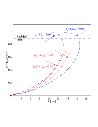
As stated in Buchdahl (1959b), Buchdahl constructed a critical constraint on stable stellar configurations that places an upper limit on the , i.e., . Notably, such boundary was initially developed for spherically symmetric isotropic (or slightly anisotropic) solutions inside GR.However, subsequent investigations have revealed that such constraints could be violated by an abundance of at least a single or many of these presumptions. With regard to stronger anisotropic models that are more realistic, the compactness can approach the limit of black hole, i.e., , also within the framework of GR, as demonstrated in Alho et al. (2022a). intriguingly, other limits impose more strict limits on in cases featuring strong anisotropy, as indicated in Alho et al. (2022b); Roupas and Nashed (2020); Raposo et al. (2019); Cardoso and Pani (2019). A similar conclusion has been reached when exploring scenarios involving nonminimal coupling between matter and geometry (Nashed and Hanafy, 2022).
Within this context, it is worthwhile to look into this constraint in the context of of gravity, as this study does. For generalized theory of gravity, the Buchdahl limit is expressed as detailed in Goswami et al. (2015).
In this study where, , for the compactness, we express the modified Buchdahl upper limit as
| (32) |
We repeat that where being the radius of the NS km. Clearly Eq.(32) reduces to Buchdahl’s GR if Buchdahl (1959b).
The Buchdahl limit for the pulsar SAX J1748.9-2021 can be computed as follows: We find for , and for , which different from GR.
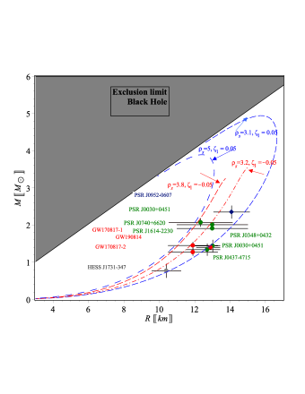
We provide the corresponding MR relation in Fig. 87(b) when ,where the matching condition (17) determines ; that is, . This refers to the optimal EoS that was previously derived in this section. Consequently, we use and the boundary density g/cm3. This results in a maximal mass with km. With and a boundary density of g/cm3, the maximum mass is obtained at a radius of km. Furthermore, we employ alternative boundary density values that yield a better fit with other pulsars while remaining consistent with the pulsar SAX J1748.9-2021, as shown in Fig. 87(b). Based on and the boundary density g/cm3, the maximum mass is found at radius km. With and g/cm3, the maximum mass at radius km is . The MR curves clearly do not extend to the limit of black hole for positive cases, as depicted by the grey region in Fig. 87(b).
VI Discussion and Conclusions
Several captivating and noteworthy discoveries emerge as soon as we delve into the realm of NSs within the framework of theory of gravity. In our exploration, we placed our primary emphasis on the particular model put forth as , and scrutinized its ramifications on the structural integrity and stability characteristics of neutron stars. To summarize our results:
-
•
We investigated how gravity (with ) models alters the conventional understanding of neutron stars as described by GR. Examining the function, we discovered that such adjustments can wield a substantial influence on the composition and dynamics of neutron stars. Our examination delved with the more practical setting of an anisotropic fluid behavior, assuming that the KB ansatz is followed by the inner region of the spherically symmetric stellar model. Concretely, we employed precise measurements derived from the radius and mass of star SAX J1748.9-2021, which boasts a mass of and a radius within the range of km. These measurements served as valuable constraints on the parameter space of our current model, specifically influencing the value of .
-
•
One of our central concerns revolved around assessing the stability of neutron star configurations within the context of gravity. We conducted an exhaustive analysis of various stability criteria, including the Zeldovich condition, energy conditions, and the speed of sound. Our results showed that theory of gravity can verify these stipulations for certain parameter ranges. As we investigated, the allowable zone of theory parameter, is given by . Different criteria of stability applied to our model from the viewpoint of geometry and matter confirmed its validity. Regarding the central density of pulsar SAX J1748.9-2021, our predictions are: When , g/cm3, that is 2.8 times the nuclear density (). Conversely, for , g/cm3, that is 2.5 times the nuclear density.
-
•
In the frame of theory, we derived the MR curve for NSs. Our results confirmed that NS mass and radius might be differ from the predictions of GR relying on how the form of . Such differences have critical consequences on the astrophysical observations and could be employ to calculate the validity of . More specific, we calculate the maximal mass corresponding to a radius of km when and a surface density of g/cm3. On the other hand, we derive the maximal mass of with a corresponding radius km when and a surface density g/cm3. Such findings are consistent with the properties of pulsar SAX J1748.9-2021 Nashed (2023).
-
•
We discussed the anisotropic properties and causality criteria of NSs in the frame of . Our discoveries revealed that, even in the presence of modifications, the speed of sound remains consistent with causality constraints. We observed that the combined effects of strong anisotropy and gravity, particularly when is negative, act to counteract gravitational collapse and successfully lower the pulsar fluid’s sound speed. Such results of maximal , is , at the center of the neutron star. This finding aligns more closely with the soft EoSs predicted by gravitational wave observations, indicating a better agreement with astrophysical reality.
-
•
In this study we show that the effect of anisotropy and within KB ansatz the pulsar could have exceed mass than that of GR. This case is similar to the isotropic case presented in Astashenok et al. (2021c) where the authors show that the maximum baryonic mass can exceed gravitational mass for for static NSs in the frame of .
In conclusion, our investigation implies that gravity offers a fresh and captivating perspective for comprehending neutron stars. Although this realm of study continues to evolve, our results suggest that the gravity frameworks can align with both theoretical stability criteria and empirical observations. The future exploration of this domain holds the promise of fine-tuning and scrutinizing these models more rigorously, potentially unveiling new revelations about the fundamental characteristics of gravity and the dynamics of compact objects such as neutron stars.
Acknowledgements
SC acknowledges the Istituto Nazionale di Fisica Nucleare (INFN) Sez. di Napoli, Iniziative Specifiche QGSKY and MOONLIGHT2 for the support. This paper is based upon work from COST Action CA21136 Addressing observational tensions in cosmology with systematics and fundamental physics (CosmoVerse) supported by COST (European Cooperation in Science and Technology).
References
- Will (2014) C. M. Will, Living reviews in relativity 17, 1 (2014).
- Abbott et al. (2018) B. P. Abbott et al., Physical review letters 121, 129902 (2018).
- Abbott et al. (2019) B. P. Abbott, R. Abbott, T. Abbott, F. Acernese, K. Ackley, C. Adams, T. Adams, P. Addesso, R. X. Adhikari, V. B. Adya, et al., Physical review letters 123, 011102 (2019).
- Starobinsky (1980) A. A. Starobinsky, Physics Letters B 91, 99 (1980).
- Capozziello (2002) S. Capozziello, International Journal of Modern Physics D 11, 483 (2002).
- Carroll et al. (2004) S. M. Carroll, V. Duvvuri, M. Trodden, and M. S. Turner, Phys. Rev. D 70, 043528 (2004), eprint astro-ph/0306438.
- Hu and Sawicki (2007) W. Hu and I. Sawicki, Phys. Rev. D 76, 064004 (2007), eprint 0705.1158.
- Nojiri and Odintsov (2006) S. Nojiri and S. D. Odintsov, eConf C0602061, 06 (2006), eprint hep-th/0601213.
- Amendola et al. (2007) L. Amendola, R. Gannouji, D. Polarski, and S. Tsujikawa, Phys. Rev. D 75, 083504 (2007), eprint gr-qc/0612180.
- Appleby and Battye (2007) S. A. Appleby and R. A. Battye, Phys. Lett. B 654, 7 (2007), eprint 0705.3199.
- Odintsov and Oikonomou (2020) S. D. Odintsov and V. K. Oikonomou, Phys. Rev. D 101, 044009 (2020), eprint 2001.06830.
- Koyama (2016) K. Koyama, Rept. Prog. Phys. 79, 046902 (2016), eprint 1504.04623.
- Nojiri and Odintsov (2003) S. Nojiri and S. D. Odintsov, Phys. Rev. D 68, 123512 (2003), eprint hep-th/0307288.
- Nojiri and Odintsov (2008) S. Nojiri and S. D. Odintsov, Phys. Rev. D 77, 026007 (2008), eprint 0710.1738.
- Cognola et al. (2008) G. Cognola, E. Elizalde, S. Nojiri, S. D. Odintsov, L. Sebastiani, and S. Zerbini, Phys. Rev. D 77, 046009 (2008), eprint 0712.4017.
- Oikonomou (2021a) V. K. Oikonomou, Phys. Rev. D 103, 044036 (2021a), eprint 2012.00586.
- Oikonomou (2021b) V. K. Oikonomou, Phys. Rev. D 103, 124028 (2021b), eprint 2012.01312.
- Sotiriou and Faraoni (2010) T. P. Sotiriou and V. Faraoni, Reviews of Modern Physics 82, 451 (2010).
- De Felice and Tsujikawa (2010) A. De Felice and S. Tsujikawa, Living Reviews in Relativity 13, 1 (2010).
- Capozziello and De Laurentis (2011) S. Capozziello and M. De Laurentis, Phys. Rept. 509, 167 (2011), eprint 1108.6266.
- Nojiri and Odintsov (2011) S. Nojiri and S. D. Odintsov, Phys. Rept. 505, 59 (2011), eprint 1011.0544.
- Clifton et al. (2012) T. Clifton, P. G. Ferreira, A. Padilla, and C. Skordis, Physics reports 513, 1 (2012).
- Nojiri et al. (2017) S. Nojiri, S. Odintsov, and V. Oikonomou, Physics Reports 692, 1 (2017).
- Yazadjiev et al. (2014) S. S. Yazadjiev, D. D. Doneva, K. D. Kokkotas, and K. V. Staykov, JCAP 06, 003 (2014), eprint 1402.4469.
- Astashenok et al. (2015) A. V. Astashenok, S. Capozziello, and S. D. Odintsov, Phys. Lett. B 742, 160 (2015), eprint 1412.5453.
- Yazadjiev and Doneva (2015a) S. S. Yazadjiev and D. D. Doneva (2015a), eprint 1512.05711.
- Sbisà et al. (2020) F. Sbisà, P. O. Baqui, T. Miranda, S. E. Jorás, and O. F. Piattella, Phys. Dark Univ. 27, 100411 (2020), eprint 1907.08714.
- Astashenok et al. (2020) A. V. Astashenok, S. Capozziello, S. D. Odintsov, and V. K. Oikonomou, Phys. Lett. B 811, 135910 (2020), eprint 2008.10884.
- Astashenok et al. (2021a) A. V. Astashenok, S. Capozziello, S. D. Odintsov, and V. K. Oikonomou, Phys. Lett. B 816, 136222 (2021a), eprint 2103.04144.
- Astashenok et al. (2021b) A. V. Astashenok, S. Capozziello, S. D. Odintsov, and V. K. Oikonomou, EPL 134, 59001 (2021b), eprint 2106.01234.
- Nobleson et al. (2022) K. Nobleson, A. Ali, and S. Banik, Eur. Phys. J. C 82, 32 (2022).
- Jiménez et al. (2022) J. C. Jiménez, J. M. Z. Pretel, E. S. Fraga, S. E. Jorás, and R. R. R. Reis, JCAP 07, 017 (2022), eprint 2112.09950.
- Abbott et al. (2020) R. Abbott, T. Abbott, S. Abraham, F. Acernese, K. Ackley, C. Adams, R. X. Adhikari, V. Adya, C. Affeldt, M. Agathos, et al., The Astrophysical Journal Letters 896, L44 (2020).
- Nashed and Saridakis (2020) G. G. L. Nashed and E. N. Saridakis, Phys. Rev. D 102, 124072 (2020), eprint 2010.10422.
- Astashenok and Odintsov (2020a) A. V. Astashenok and S. D. Odintsov, Mon. Not. Roy. Astron. Soc. 493, 78 (2020a), eprint 2001.08504.
- Astashenok and Odintsov (2020b) A. V. Astashenok and S. D. Odintsov, Mon. Not. Roy. Astron. Soc. 498, 3616 (2020b), eprint 2008.11271.
- Olmo et al. (2020) G. J. Olmo, D. Rubiera-Garcia, and A. Wojnar, Physics Reports 876, 1 (2020).
- Boehmer et al. (2008) C. G. Boehmer, T. Harko, and F. S. N. Lobo, Astropart. Phys. 29, 386 (2008), eprint 0709.0046.
- Sharma et al. (2021) V. K. Sharma, B. K. Yadav, and M. M. Verma, Eur. Phys. J. C 81, 109 (2021), eprint 2011.02878.
- Capozziello et al. (2006) S. Capozziello, V. F. Cardone, and A. Troisi, Phys. Rev. D 73, 104019 (2006), eprint astro-ph/0604435.
- Nashed (2018) G. G. L. Nashed, Adv. High Energy Phys. 2018, 7323574 (2018).
- Capozziello et al. (2007) S. Capozziello, V. F. Cardone, and A. Troisi, Mon. Not. Roy. Astron. Soc. 375, 1423 (2007), eprint astro-ph/0603522.
- Martins and Salucci (2007) C. F. Martins and P. Salucci, Mon. Not. Roy. Astron. Soc. 381, 1103 (2007), eprint astro-ph/0703243.
- Nashed and Nojiri (2020) G. G. L. Nashed and S. Nojiri, Phys. Rev. D 102, 124022 (2020), eprint 2012.05711.
- Jaryal and Chatterjee (2021) S. C. Jaryal and A. Chatterjee, Eur. Phys. J. C 81, 273 (2021), eprint 2102.08717.
- Sharma and Verma (2022) A. K. Sharma and M. M. Verma, Astrophys. J. 926, 29 (2022).
- Capozziello et al. (2016) S. Capozziello, M. De Laurentis, R. Farinelli, and S. D. Odintsov, Phys. Rev. D 93, 023501 (2016), eprint 1509.04163.
- Chaichian et al. (2000) M. Chaichian, S. S. Masood, C. Montonen, A. Perez Martinez, and H. Perez Rojas, Phys. Rev. Lett. 84, 5261 (2000), eprint hep-ph/9911218.
- Ferrer et al. (2010) E. J. Ferrer, V. de la Incera, J. P. Keith, I. Portillo, and P. L. Springsteen, Phys. Rev. C 82, 065802 (2010), eprint 1009.3521.
- Horvat et al. (2011) D. Horvat, S. Ilijic, and A. Marunovic, Class. Quant. Grav. 28, 025009 (2011), eprint 1010.0878.
- Doneva and Yazadjiev (2012) D. D. Doneva and S. S. Yazadjiev, Phys. Rev. D 85, 124023 (2012), eprint 1203.3963.
- Silva et al. (2015) H. O. Silva, C. F. Macedo, E. Berti, and L. C. Crispino, Classical and Quantum Gravity 32, 145008 (2015).
- Yagi and Yunes (2015) K. Yagi and N. Yunes, Phys. Rev. D 91, 123008 (2015), eprint 1503.02726.
- Ivanov (2017) B. Ivanov, The European Physical Journal C 77, 1 (2017).
- Isayev (2017) A. Isayev, Physical Review D 96, 083007 (2017).
- Biswas and Bose (2019) B. Biswas and S. Bose, Physical Review D 99, 104002 (2019).
- Maurya et al. (2019) S. K. Maurya, A. Banerjee, M. K. Jasim, J. Kumar, A. K. Prasad, and A. Pradhan, Phys. Rev. D 99, 044029 (2019), eprint 1811.09890.
- Pretel (2020) J. M. Pretel, The European Physical Journal C 80, 726 (2020).
- Rahmansyah et al. (2020) A. Rahmansyah, A. Sulaksono, A. B. Wahidin, and A. M. Setiawan, Eur. Phys. J. C 80, 769 (2020).
- Das et al. (2021a) S. Das, S. Ray, M. Khlopov, K. Nandi, and B. K. Parida, Annals of Physics 433, 168597 (2021a).
- Das et al. (2021b) S. Das, K. N. Singh, L. Baskey, F. Rahaman, and A. K. Aria, General Relativity and Gravitation 53, 1 (2021b).
- Deb et al. (2021) D. Deb, B. Mukhopadhyay, and F. Weber, Astrophys. J. 922, 149 (2021), eprint 2108.12436.
- Rahmansyah and Sulaksono (2021) A. Rahmansyah and A. Sulaksono, Phys. Rev. C 104, 065805 (2021).
- Bordbar and Karami (2022) G. H. Bordbar and M. Karami, The European Physical Journal C 82, 74 (2022).
- Folomeev (2018) V. Folomeev, Physical Review D 97, 124009 (2018).
- Panotopoulos et al. (2021) G. Panotopoulos, T. Tangphati, A. Banerjee, and M. K. Jasim, Phys. Lett. B 817, 136330 (2021), eprint 2104.00590.
- Nashed et al. (2021) G. Nashed, S. D. Odintsov, and V. Oikonomou, The European Physical Journal C 81, 528 (2021).
- Shamir and Malik (2021) M. F. Shamir and A. Malik, Chin. J. Phys. 69, 312 (2021).
- Malik et al. (2022a) A. Malik, A. Ashraf, U. Naqvi, and Z. Zhang, Int. J. Geom. Meth. Mod. Phys. 19, 2250073 (2022a).
- Farasat Shamir and Malik (2019) M. Farasat Shamir and A. Malik, Commun. Theor. Phys. 71, 599 (2019).
- Nashed and El Hanafy (2023) G. G. L. Nashed and W. El Hanafy (2023), eprint 2306.13396.
- Malik (2022) A. Malik, New Astron. 93, 101765 (2022).
- Malik et al. (2022b) A. Malik, I. Ahmad, and Kiran, Int. J. Geom. Meth. Mod. Phys. 19, 2250028 (2022b).
- Usman and Shamir (2022) A. Usman and M. F. Shamir, New Astron. 91, 101691 (2022).
- Ahmad et al. (2021) M. Ahmad, G. Mustafa, and M. F. Shamir, Int. J. Mod. Phys. A 36, 2150203 (2021).
- Nashed and Capozziello (2020) G. G. Nashed and S. Capozziello, The European Physical Journal C 80, 1 (2020).
- Roupas and Nashed (2020) Z. Roupas and G. G. Nashed, The European Physical Journal C 80, 1 (2020).
- Krori and Barua (1975) K. D. Krori and J. Barua, Journal of Physics A 8, 508 (1975).
- Özel et al. (2009) F. Özel, T. Güver, and D. Psaltis, The Astrophysical Journal 693, 1775 (2009).
- Yazadjiev and Doneva (2015b) S. S. Yazadjiev and D. D. Doneva (2015b), eprint 1512.05711.
- Buchdahl (1959a) H. A. Buchdahl, Physical Review 116, 1027 (1959a).
- Ivanov (2002) B. V. Ivanov, Physical Review D 65, 104011 (2002).
- Barraco et al. (2003) D. E. Barraco, V. H. Hamity, and R. J. Gleiser, Physical Review D 67, 064003 (2003).
- Böhmer and Harko (2006) C. Böhmer and T. Harko, Classical and Quantum Gravity 23, 6479 (2006).
- Legred et al. (2021) I. Legred, K. Chatziioannou, R. Essick, S. Han, and P. Landry, Phys. Rev. D 104, 063003 (2021), eprint 2106.05313.
- Zeldovich and Novikov (1971) Y. B. Zeldovich and I. D. Novikov, Relativistic astrophysics. Vol. 1: Stars and relativity, Chicago: University of Chicago Press (1971).
- Capozziello et al. (2015) S. Capozziello, F. S. N. Lobo, and J. P. Mimoso, Phys. Rev. D 91, 124019 (2015), eprint 1407.7293.
- Herrera (1992) L. Herrera, Phys. Lett. A 165, 206 (1992).
- Chandrasekhar (1964) S. Chandrasekhar, Astrophys. J. 140, 417 (1964), [Erratum: Astrophys.J. 140, 1342 (1964)].
- Chan et al. (1993) R. Chan, L. Herrera, and N. Santos, Monthly Notices of the Royal Astronomical Society 265, 533 (1993).
- Heintzmann and Hillebrandt (1975) H. Heintzmann and W. Hillebrandt, Astronomy and Astrophysics 38, 51 (1975).
- Tolman (1930) R. C. Tolman, Physical Review 35, 896 (1930).
- Buchdahl (1959b) H. A. Buchdahl, Phys. Rev. 116, 1027 (1959b), URL https://link.aps.org/doi/10.1103/PhysRev.116.1027.
- Alho et al. (2022a) A. Alho, J. Natário, P. Pani, and G. Raposo, Phys. Rev. D 106, L041502 (2022a), eprint 2202.00043.
- Alho et al. (2022b) A. Alho, J. Natário, P. Pani, and G. Raposo, Phys. Rev. D 105, 044025 (2022b), [Erratum: Phys.Rev.D 105, 129903 (2022)], eprint 2107.12272.
- Raposo et al. (2019) G. Raposo, P. Pani, M. Bezares, C. Palenzuela, and V. Cardoso, Phys. Rev. D 99, 104072 (2019), eprint 1811.07917.
- Cardoso and Pani (2019) V. Cardoso and P. Pani, Living Rev. Rel. 22, 4 (2019), eprint 1904.05363.
- Nashed and Hanafy (2022) G. Nashed and W. E. Hanafy, The European Physical Journal C 82, 679 (2022).
- Goswami et al. (2015) R. Goswami, S. D. Maharaj, and A. M. Nzioki, Phys. Rev. D 92, 064002 (2015), eprint 1506.04043.
- Nashed (2023) G. G. L. Nashed, Astrophys. J. 950, 129 (2023), eprint 2306.10273.
- Astashenok et al. (2021c) A. V. Astashenok, S. Capozziello, S. D. Odintsov, and V. K. Oikonomou, EPL 136, 59001 (2021c), eprint 2111.14179.