A multiscale hybrid Maxwellian-Monte-Carlo Coulomb collision algorithm for particle simulations

Abstract

Coulomb collisions in particle simulations for weakly coupled plasmas are modeled by the Landau-Fokker-Planck equation, which is typically solved by Monte-Carlo (MC) methods. One of the main disadvantages of MC is the timestep accuracy constraint ν$\Delta$t $\ll$ 1 to resolve the collision frequency ν. The constraint becomes extremely stringent for self-collisions in the presence of high charge state species and for inter-species collisions with large mass disparities (such as present in Inertial Confinement Fusion hohlraums), rendering long-time-scale simulations prohibitively expensive or impractical. To overcome these difficulties, we explore a hybrid Maxwellian-MC (HMMC) model for particle simulations. Specifically, we devise a collisional algorithm that describes weakly collisional species with particles, and highly collisional species and fluid components with Maxwellians. We employ the Lemons method for particle-Maxwellian collisions, enhanced with a more careful treatment of low-relative-speed particles, and a five-moment model for Maxwellian-Maxwellian collisions. Particle-particle binary collisions are dealt with classic Takizuka-Abe MC, which we extend to accommodate arbitrary particle weights to deal with large density disparities without compromising conservation properties. HMMC is strictly conservative and significantly outperforms standard MC methods in situations with large mass disparities among species or large charge states, demonstrating orders of magnitude improvement in computational efficiency. We will substantiate the accuracy and performance of the proposed method with several examples of varying complexity, including both zero-dimensional relaxation and one-dimensional transport problems, the latter using a hybrid kinetic-ion/fluid-electron model.

1 Introduction

In numerous laboratory and natural plasma applications, such as magnetic and inertial fusion, space plasmas, and low-temperature plasma discharges, there is a growing demand for reliable, long-time-scale kinetic simulations that accurately account for Coulomb collisions. Our focus is on Coulomb collisions in fully ionized, non-relativistic, weakly coupled plasmas, which are typically described by the Landau-Fokker-Planck (LFP) equation [1].

Conventional collisional approaches typically fall into two main categories: particle-based and grid-based methods. Particle-based collision methods are particularly attractive for implementation in particle-in-cell (PIC) algorithms owing to their flexibility and widespread use. Among these, particle-pairing methods utilizing Monte Carlo (MC) techniques [2, 3] are most widely adopted. The MC method offers several advantages, including a linear cost scaling with the number of particles $N_{p}$, straightforward implementations, automatic preservation of positivity, and the strict conservation of mass, momentum, and energy. Integration with PIC methods are typically achieved through first-order operator splitting, resulting in robust PIC-MC simulation algorithms.

However, standard MC methods exhibit several limitations. Their temporal convergence rate is typically slow ($\sim\sqrt{\Delta t}$) [4, 5]. Their random character introduces additional noise in already noisy particle simulations, exacerbating errors. Another drawback of MC is the timestep constraint ($\nu\Delta t\ll 1$) to resolve all collision frequencies $\nu$ for accuracy [4, 5]. The timestep constraint becomes particularly challenging for self-collisions involving high-Z species (as $\nu\propto Z^{4}$), and for inter-species collisions with significant mass disparities (as $\nu\propto m_{\alpha\beta}^{-1}$ where the reduced mass $m_{\alpha\beta}$ will be approximately equal to the smaller mass), rendering such simulations prohibitively expensive. These challenges have motivated researchers to investigate alternative approaches for disparate-mass collisions based on Langevin stochastic models for particle-Maxwellian collisions [6, 7, 8].

Other authors have attempted to accelerate MC for Coulomb collisions either by considering splitting the distribution function into one or several Maxwellian components plus a kinetic one [9, 10, 7, 11, 12], or by using multilevel MC methods [13]. The method most closely related to this study is the so-called hybrid MC method, introduced by Caflisch [10] and later improved by Ricketson [11]. In these approaches, the particle distribution function is decomposed into a Maxwellian component (described analytically) plus a perturbation (described with particles). As in our proposed algorithm, the computational speedup follows from the fact that the Maxwellian self-collisions are null, and no longer introduce a fast timescale. However, the actual implementation of these approaches is cumbersome, as they explicitly need to thermalize/dethermalize particles to keep the Maxwellian component a Maxwellian during the collisional evolution.

Other authors have proposed deterministic particle collisional algorithms that sidestep MC altogether, avoiding random noise [14, 15, 16, 17, 18]. These methods employ a gradient-flow formulation to derive equations of motion for the particles, which encode the collisional process with high fidelity and preserve all collisional invariants (mass, momentum, and energy) with implicit timestepping [16] while guaranteeing an H-theorem for entropy generation. As a result, they result in noise-free particle collision simulations. However, these methods remain expensive, of $\mathcal{O}(N_{p}^{2})$, are typically implemented explicitly in time (breaking energy conservation), and so far require a velocity-space mesh for initialization due to the particle regularization employed, which is subject to the curse of dimensionality. Random batching [15, 18] can significantly ameliorate the computational scaling to $\mathcal{O}(N_{p}^{2}/R)$, with $R$ the number of random batches, without formal loss of conservation properties. However, accuracy considerations require that $R$ scale sublinearly with $N_{p}$ [15], as well as a sufficiently small timestep to recover collision statistics. Therefore, despite significant acceleration, at present the approach scales superlinearly with $N_{p}$ and is not multiscale in time, needing to resolve all collisional time scales present.

Coulomb collisional methods utilizing a velocity grid have also been extensively explored (see Ref. [19] and references therein for a good survey). Implicit time integration enables stepping over stiff collisional timescales, with the potential of significant efficiency gains while preserving all relevant conservation properties, either directly with the LFP formulation [20, 21, 22, 23, 24] or the equivalent Rosenbluth-Fokker-Planck one [19, 25, 26, 27, 28]. Conservation in the Landau form arises from symmetry, and is straightforward to enforce, but the method is $\mathcal{O}(N^{2}),$ with $N$ the total number of mesh points. In contrast, the Rosenbluth form can be made $\mathcal{O}(N)$, but ensuring the conservation laws and constraints for long-term accuracy necessitates specialized techniques, which can be intricate [19, 25, 26, 27, 28]. Acceleration techniques are indispensable to improve the convergence rate of nonlinear iterative solvers required by the resulting nonlinear algebraic systems, especially when dealing with stiff timescales, a task that presents its own set of challenges [28]. In addition to the temporal integration challenges, attempting to solve the LFP equation on a three-dimensional velocity grid quickly leads to the so-called curse of dimensionality of tensor-product meshes in high-dimensions when coupled with Vlasov’s equation, rendering it expensive for long-time applications on even today’s fastest supercomputers. Grid-based collisional methods can be combined with PIC simulations [23] to avoid random MC noise. However, the frequent interpolations between the phase-space grid and the particles can lead to numerical diffusion [29] unless specialized interpolation techniques are employed [30].

This study proposes a hybrid Maxwellian-MC (HMMC) Coulomb-collision approach in which colliding species can be described by either particles or Maxwellians, the latter being an appropriate description under the assumption of sufficiently fast self-collisions. As in earlier hybrid MC approaches [10, 11], treating fast-colliding species as a Maxwellian eliminates the fastest self-collisional timescales of the system, resulting in significant algorithmic speedups. However, unlike those earlier studies, our approach does not require particle (de)thermalization because we only use the Maxwellian ansatz when the collisionality regime warrants it. The approach considers all types of collisions: among particles, among Maxwellians, and between particles and Maxwellians. It scales as $\mathcal{O}(N_{p})$ and strictly conserves all collisional invariants. Our approach offers a completely general multiscale solution for arbitrary particle systems undergoing Coulombian interactions, but is particularly suitable for hybrid fluid-PIC algorithms (where electrons are commonly modeled by a fluid species) and for systems featuring high-Z ion species because the self-collision frequency scales as $Z^{4}$, and classical MC methods quickly become expensive.

Since our approach considers coexisting particle and fluid species, collisions between particles, between particles and Maxwellians, and between Maxwellians need an appropriate treatment. Here, we employ the Takizuka-Abe (TA) MC method [2] for particle-particle binary collisions, the Lemons method [7] for particle-Maxwellian collisions, and the 5-moment model for collisions between Maxwellian species [31, 32]. Importantly, we enhance the Lemons method with a more careful treatment of low-relative-speed particles, without which the method may either produce erroneous results or be very inefficient [5]. Moreover, we also extend the standard TA method to accommodate arbitrary particle weights without compromising conservation properties. This can be particularly useful for collisions between species with large density disparities. Previous studies on variable-weight Coulomb collision schemes were often developed in an ad-hoc manner, with a primary focus on conserving momentum and energy on average [33, 34, 35, 36]. However, there are notable exceptions to this trend. Shanny et al. derived their scheme specifically for simulating electrons in electron-ion collisions [37]. Tanaka et al., on the other hand, introduced a correction step aimed at achieving exact momentum and energy conservation. However, they did not provide a detailed derivation of their proposed particle pairing scheme [38]. The proposed method is strictly conservative in mass, momentum, and energy, and as we will show significantly outperforms classical MC methods, with orders of magnitude improvement vs. TA in computational efficiency. We will substantiate the accuracy and performance of the proposed method with several examples of varying complexity, including both relaxation and transport problems.

This paper is organized as follows. Section 2 introduces the three models utilized in this study for particle-particle, particle-Maxwellian, and Maxwellian-Maxwellian collisions. In Sec. 3, HMMC is demonstrated with various difficult benchmarks, including zero-dimensional multi-species relaxation and one-dimensional multi-species transport in an Inertial Confinement Fusion (ICF) hohlraum-like environment. Finally, we summarize the study and conclude in Sec. 4.

2 Methodology

We aim for a versatile multiscale collisional particle algorithm that allows any highly collisional species to be represented as a Maxwellian during the collision process. This, in turn, requires suitable algorithmic solutions to deal with particle-particle, particle-Maxwellian, and Maxwellian-Maxwellian collisions.

For particle-particle collisions, we consider the well-known TA algorithm. However, the conventional TA model encounters challenges when dealing with collisions between species with significant density disparities. This often occurs in scenarios where a species is moving into an empty space or when the system contains a minority species. The TA algorithm assumes a uniform particle weight between collision pairs, which can lead to either an excessive number of particles for the high-density species or an inadequate number for the low-density ones, resulting in efficiency issues or enhanced noise, respectively. To circumvent these difficulties, non-uniform weight schemes are preferred [33, 34, 35, 36]. In this study, we devised a new particle pairing scheme for non-uniform TA collisions, incorporating a correction step to ensure exact conservation of momentum and energy. This approach addresses the shortcomings of the conventional TA model and enhances the accuracy and efficiency of particle-particle collision treatments in strongly non-uniform plasma systems.

Particle-Maxwellian collisions are dealt with an improved version of the Lemons algorithm [7]. The Lemons method, formulated in spherical coordinates, has proven to be more efficient than Cartesian Langevin equations [5] in scenarios where a light particle species collides with a heavy Maxwellian species, making it a more palatable choice. Additionally, we have fixed a failure mode that we uncovered in the treatment of low-relative-speed particles in the standard Lemons algorithm that renders the method accurate for virtually any particle-Maxwellian interaction.

Maxwellian-Maxwellian collisions are modeled with a five-moment model describing the evolution of the Maxwellian moments. The 5-moment equations are derived exactly by moment integration of the LFP equation when assuming the Maxwellian remains so dynamically, and can be shown to preserve all conservation properties exactly [31, 32]. The 5-moment model eliminates self-collisional timescales from the formulation, which is particularly advantageous when dealing with stiff self-colliding species.

In the following sub-sections, we discuss first the Maxwellian-Maxwellian collision method, next the improved Lemons method, and last the extended TA method. We also discuss the special case of hybrid kinetic-ion/fluid-electron algorithms [39], which is a common model of choice for various applications, and demands a specialized treatment of the fluid electron system to ensure strict conservation properties of collisional invariants [6]. Finally, we briefly comment on the algorithmic orchestration such that conservation properties are preserved during the whole collisional step.

2.1 Maxwellian-Maxwellian collisions: 5-moment model

A three-dimensional Maxwellian distribution function is fully determined by its first five moments ($n,\boldsymbol{u},T$), and may be written as:

$$\varphi(\mathbf{v})=n\left(\frac{m}{2\pi kT}\right)^{3/2}\exp\left(-\frac{m(\mathbf{v}-\mathbf{u})^{2}}{2kT}\right),$$

where the five moments are defined as:

$$n =\int\varphi(\mathbf{v})d\mathbf{v},$$

$$\mathbf{u} =\frac{1}{n}\int\varphi(\mathbf{v})\mathbf{v}d\mathbf{v},$$

$$T =\frac{m}{3kn}\int\varphi(\mathbf{v})(\mathbf{v}-\mathbf{u})^{2}d\mathbf{v}.$$

Here, $m$ is mass, $k$ is the Boltzmann constant. If we further assume that the Maxwellian is preserved during the collision process (so-called 5-moment approximation), then the evolution equations for the moments undergoing Coulomb collisions can be exactly formulated. This is done by taking the moments of the Landau-Fokker-Planck equation, resulting in the following equations of motion for the moments of the Maxwellian distribution [31, 32]:

$$\frac{dn_{\alpha}}{dt} =0,$$ (1)

$$\frac{d\mathbf{u}_{\alpha}}{dt} =\sum_{\beta}\nu_{\alpha\beta}(\mathbf{u}_{\beta}-\mathbf{u}_{\alpha})\Phi_{\alpha\beta},$$ (2)

$$\frac{3}{2}k\frac{dT_{\alpha}}{dt} =\sum_{\beta}\frac{m_{\alpha}}{m_{\alpha}+m_{\beta}}\nu_{\alpha\beta}\left[3k(T_{\beta}-T_{\alpha})\Psi_{\alpha\beta}+m_{\beta}(\mathbf{u}_{\beta}-\mathbf{u}_{\alpha})^{2}\Phi_{\alpha\beta}\right],$$ (3)

where

$$\nu_{\alpha\beta} =\frac{1}{3}\frac{n_{\beta}m_{\beta}}{m_{\alpha}+m_{\beta}}\left(\frac{2\pi kT_{\alpha\beta}}{m_{\alpha\beta}}\right)^{-3/2}\frac{e_{\alpha}^{2}e_{\beta}^{2}}{\varepsilon_{0}^{2}m_{\alpha\beta}^{2}}\mathrm{ln}\Lambda,$$

$$m_{\alpha\beta} =\frac{m_{\alpha}m_{\beta}}{m_{\alpha}+m_{\beta}},$$

$$T_{\alpha\beta} =\frac{m_{\beta}T_{\alpha}+m_{\alpha}T_{\beta}}{m_{\alpha}+m_{\beta}},$$

$$\Phi_{\alpha\beta} =\frac{3}{2u_{\alpha\beta}^{2}}\left(\frac{\sqrt{\pi}}{2}\frac{\phi(u_{\alpha\beta})}{u_{\alpha\beta}}-\exp(-u_{\alpha\beta}^{2})\right),$$

$$\Psi_{\alpha\beta} =\exp(-u_{\alpha\beta}^{2}),$$

$$u_{\alpha\beta} =\frac{|\mathbf{u}_{\alpha}-\mathbf{u}_{\beta}|}{\sqrt{2kT_{\alpha\beta}/m_{\alpha\beta}}},$$

and $\phi(x)=\frac{2}{\sqrt{\pi}}\int_{0}^{x}e^{-y^{2}}dy$ is the error function. To facilitate a conservative discretization of the energy equation, we reformulate Eq. 3 in terms of the energy $\varepsilon_{\alpha}=\frac{1}{2}m_{\alpha}u_{\alpha}^{2}+\frac{3}{2}kT_{\alpha}$ as:

$$\frac{d\varepsilon_{\alpha}}{dt}=\sum_{\beta}\frac{m_{\alpha}\mathbf{u}_{\alpha}+m_{\beta}\mathbf{u}_{\beta}}{m_{\alpha}+m_{\beta}}m_{\alpha}\nu_{\alpha\beta}(\mathbf{u}_{\beta}-\mathbf{u}_{\alpha})\Phi_{\alpha\beta}+\frac{m_{\alpha}3k(T_{\beta}-T_{\alpha})}{m_{\alpha}+m_{\beta}}\nu_{\alpha\beta}\Psi_{\alpha\beta}.$$ (4)

We employ the following time-centered discretization of Eqs. 2 and 4:

$$\frac{\mathbf{u}_{\alpha}^{n+1}-\mathbf{u}_{\alpha}^{n}}{\Delta t} =\sum_{\beta}\left(\nu_{\alpha\beta}(\mathbf{u}_{\beta}-\mathbf{u}_{\alpha})\Phi_{\alpha\beta}\right)^{n+1/2},$$

$$\frac{\varepsilon_{\alpha}^{n+1}-\varepsilon_{\alpha}^{n}}{\Delta t} =\sum_{\beta}\left(\frac{m_{\alpha}\mathbf{u}_{\alpha}+m_{\beta}\mathbf{u}_{\beta}}{m_{\alpha}+m_{\beta}}m_{\alpha}\nu_{\alpha\beta}(\mathbf{u}_{\beta}-\mathbf{u}_{\alpha})\Phi_{\alpha\beta}+\frac{m_{\alpha}3k(T_{\beta}-T_{\alpha})}{m_{\alpha}+m_{\beta}}\nu_{\alpha\beta}\Psi_{\alpha\beta}\right)^{n+1/2},$$

with the right-hand-side computed with all quantities averaged between times $n$ and $n+1$. It is straightforward to see that conservation of momentum and energy follow by symmetry:

$$\sum_{\alpha}(\mathbf{u}_{\alpha}^{n+1}-\mathbf{u}_{\alpha}^{n}) =0,$$

$$\sum_{\alpha}(\varepsilon_{\alpha}^{n+1}-\varepsilon_{\alpha}^{n}) =0.$$

Since the formulae were first derived by Burgers [31], hereafter we call it the Burgers method.

2.2 Particle-Maxwellian collisions: improved Lemons method

The Lemons algorithm [7] is a "particle-moment" collision algorithm designed for Coulomb collisions. This method involves a set of stochastic differential equations (SDE) that account for particle collisions with a "fluid" species characterized by a Maxwellian distribution. During each timestep, particles are scattered once with a "fluid" species within a cell. The scattering process is determined using finite difference solutions to stochastic differential equations that incorporate Spitzer’s velocity space diffusion coefficients. A scattering event is characterized by changes in the deflective angle $d\theta$, azimuthal angle $d\phi$ , and relative speed $d\omega$ (note that $\omega=|\mathbf{v}_{t}-\mathbf{v}_{f}|$, with $\mathbf{v}_{t}$ the test particle velocity and $\mathbf{v}_{f}$ the fluid drift velocity; the angles ($\theta,\phi$) are defined with $\omega$ aligned with the $z$-coordinate). The time evolution of those quantities is governed by:

$$d\theta =\sqrt{2\gamma dt}N_{\theta}(0,1),$$ (5)

$$d\phi =2\pi U_{\phi}(0,1),$$ (6)

$$d\omega =-\beta\omega dt+\sqrt{\delta^{2}dt}N_{\omega}(0,1),$$ (7)

where $N_{\theta}(0,1)$ and $N_{\omega}(0,1)$ are normal random variables with zero mean and unit variance, $U_{\phi}(0,1)$ is a uniform random variable distributed between zero and one. The coefficients $\gamma$, $\beta$ and $\delta^{2}$ are found from matching Chandrasekhar’s classical formulas [40]:

$$\frac{d}{dt}\left\langle v_{z}\right\rangle =-l_{f}^{2}A_{D}(1+\frac{m_{t}}{m_{f}})G(\hat{\omega}),$$ (8)

$$\frac{d}{dt}\left(\left\langle v_{z}^{2}\right\rangle-\left\langle v_{z}\right\rangle^{2}\right) =\frac{A_{D}}{\omega_{0}}G(\hat{\omega}),$$ (9)

$$\frac{d}{dt}\left(\left\langle v_{\perp}^{2}\right\rangle-\left\langle v_{\perp}\right\rangle^{2}\right) =\frac{A_{D}}{\omega_{0}}[\phi(\hat{\omega})-G(\hat{\omega})],$$ (10)

where $\left\langle v_{z}\right\rangle$ denotes expectation value over the particle distribution, subscript $z$ denotes the direction of the relative velocity, subscript $\perp$ denotes direction perpendicular to the relative velocity, subscript $f$ and $t$ denote field and test particles respectively, $\hat{\omega}=\omega l_{f}$ with $l_{f}=\sqrt{m_{f}/2T_{f}}=1/v_{th,f}$ the inverse thermal velocity of the fluid, $\phi(x)$ is the error function, and:

$$G(x) =\frac{\phi(x)-x\phi^{\prime}(x)}{2x^{2}},$$ (11)

with $\phi^{\prime}(x)=d\phi(x)/dx$, $A_{D}=8\pi n_{f}q_{t}^{2}q_{f}^{2}\ln\Lambda/m_{t}^{2}$, and $\ln\Lambda$ the Coulomb logarithm. By expressing the dynamic friction and diffusion coefficients through equations 5-7 and comparing those with Eqs. 8-10, one finds that:

$$\gamma =\frac{A_{D}}{2\omega^{3}}[\phi(\hat{\omega})-G(\hat{\omega})],$$ (12)

$$\beta =\frac{A_{D}}{2\omega^{3}}\left\{G(\hat{\omega})\left[\left(1+\frac{m_{t}}{m_{f}}\right)2\hat{\omega}^{2}+1\right]-\phi(\hat{\omega})\right\},$$ (13)

$$\delta^{2} =\frac{A_{D}G(\hat{\omega})}{\omega}.$$ (14)

We discretize Eqs. 5-7 in time as:

$$\theta^{n+1} =\theta^{n}+\sqrt{2\gamma^{n}\Delta t}N_{\theta}(0,1),$$ (15)

$$\phi^{n+1} =\phi^{n}+2\pi U_{\phi}(0,1),$$ (16)

$$\omega^{n+1} =e^{-\beta^{n}\Delta t}\omega^{n}+\sqrt{(\delta^{n})^{2}\Delta t}N_{\omega}(0,1)+\frac{1}{2}\delta^{n}\delta^{\prime n}\Delta t\left(N_{\omega}(0,1)^{2}-1\right),$$ (17)

where $\gamma^{n}$, $\beta^{n}$, and $\delta^{n}$ are obtained by evaluating Eqs. 12-14 using the timestep $n$ quantities. Here, we employ the Milstein scheme [41] for the speed ($\omega$) update, which is a first-order strong-convergence temporal scheme. In Eq. 17,

$$\delta\delta^{\prime}=-\frac{A_{D}}{4\omega^{3/2}}\left(\phi^{\prime\prime}(\hat{\omega})+6G(\hat{\omega})\right)$$ (18)

with $\phi^{\prime\prime}(x)=-\frac{4x}{\sqrt{\pi}}e^{-x^{2}}$, and we have analytically integrated the deterministic (friction) term. We use the same normal random number for the two normal distributions in Eq. 17. The exponential integration prevents negative values from the deterministic term for any timestep, and allows relatively large timesteps without resulting in negative values from the random term. If that happens and $\omega^{n+1}<0$ for a given particle, we invoke the low-relative-speed particle treatment, which we describe next.

2.2.1 Low-relative-speed particle treatment in Lemons

We note that $\gamma$, $\beta$ and $\delta^{2}$ are singular as $\omega\rightarrow 0$. The solution provided by Lemons in Ref. [7] is to Taylor-expand for sufficiently small $\omega$ to find the leading-order terms in $\beta$ (from Eq. 13), which are then plugged into Eq. 7. Neglecting the second diffusion term in Eq. 7, we find:

$$d\omega=\frac{2A_{D}l_{f}dt}{3\sqrt{\pi}\omega},$$ (19)

which can be used to update $\omega$ as:

$$\omega(t+\Delta t)=\sqrt{\omega^{2}+\frac{4}{3\sqrt{\pi}}A_{D}l_{f}\Delta t}.$$ (20)

As noted in Ref. [7], Eq. 20 differs from the deterministic part in Eq. 7 when:

$$\omega^{2}\leq\frac{4}{3\sqrt{\pi}}A_{D}l_{f}\Delta t,$$ (21)

which provides a means to define when the $\omega$ is sufficiently small.

However, the small-$\omega$ limit holds true only under certain conditions: 1) the argument of the error and Chandrasekhar functions (i.e., $\hat{\omega}\equiv\omega l_{f}=\omega/v_{th,f}$) must also be small; and 2) it must also be small enough so that the physical response of the particle is acceleration (not deceleration). Condition 1) may become invalid when $l_{f}$ is large (i.e., for small fluid thermal velocity). But more importantly, Equation 20 always accelerates the particle, which is unphysical and eventually breaks the smallness of $\omega$ regardless of its initial value.

To fix this inconsistency, we draw inspiration from the classical TA MC algorithm [2], which proposes that scattering becomes isotropic when $\sigma^{2}=\frac{e_{\alpha}^{2}e_{\beta}^{2}n_{L}\ln\Lambda}{8\pi\epsilon_{0}m_{\alpha\beta}^{2}\omega^{3}}\Delta t>1$ (see e.g. Eq. 27 in the next section). This insight agrees with MC simulations conducted in Ref. [3], which demonstrate that isotropic scattering occurs when $s\equiv 2\sigma^{2}\gtrsim 4$, which is the criterion we adopt in this study. This condition defines a smallness threshold for $\omega$, given by:

$$\omega^{3}\lesssim\frac{e_{\alpha}^{2}e_{\beta}^{2}n_{L}\ln\Lambda}{16\pi\epsilon_{0}m_{\alpha\beta}^{2}\omega^{3}}\Delta t,$$

below which we perform isotropic scattering, thereby avoiding the singularity of Eq. 7.

To prevent the particles from always accelerating in the small-$\omega$ regime (as would be dictated by Eq. 20), we derive a more appropriate formula for determining the relative velocity by considering the averaged $\omega^{2}$. We may write:

$$d\omega^{2} =(\omega+d\omega)^{2}-\omega^{2}$$

$$=2\omega d\omega+(d\omega)^{2}$$

$$=2\omega\left(-\beta\omega dt+\sqrt{\delta^{2}dt}N_{\omega}(0,1)\right)+\left(-\beta\omega dt+\sqrt{\delta^{2}dt}N_{\omega}(0,1)\right)^{2}$$

$$=-2\beta\omega^{2}dt+2\omega\sqrt{\delta^{2}dt}N_{\omega}(0,1)+\delta^{2}dt[N_{\omega}(0,1)]^{2},$$

where we have neglected higher-order $dt$-terms. By taking the average of the above equation, we get

$$<d\omega^{2}> =-2\beta\omega^{2}dt+\delta^{2}dt$$

$$=-2A_{D}l_{f}\left(\frac{m_{t}}{m_{f}}\hat{\omega}G(\hat{\omega})-\frac{e^{-\hat{\omega}^{2}}}{\sqrt{\pi}}\right)dt.$$ (22)

Since low-relative-speed particles will experience a large number of small-angle collisions, the accumulated effect can be modeled as isotropic scattering [3]. By approximating $<d\omega^{2}>/dt\approx d\omega^{2}/dt$, we aim at counting the average energy exchange between the particle and the field distribution, and finally get:

$$\frac{d\omega^{2}}{dt}=-2A_{D}l_{f}\left(\frac{m_{t}}{m_{f}}\hat{\omega}G(\hat{\omega})-\frac{e^{-\hat{\omega}^{2}}}{\sqrt{\pi}}\right)=S.$$ (23)

In this study, we solve Eq. 23 with a predictor-corrector scheme, written as:

$$\frac{(\omega^{2})^{*}-(\omega^{2})^{n}}{\Delta t} =S^{n},$$ (24)

$$\frac{(\omega^{2})^{**}-(\omega^{2})^{*}}{\Delta t} =S^{*},$$ (25)

where the superscript * indicates the predicted solution using the $S$ (the right hand side of Eq. 23) evaluated at time level $n$, while the corrected solution (indicated by the superscript **) is obtained from $S$ evaluated using $\omega^{*}$. The final solution is found as the temporal average of the two:

$$\omega^{n+1}=\frac{\omega^{*}+\omega^{**}}{2}.$$ (26)

After the collision process, the coordinate reference is changed back from the $z$-aligned $\omega$ to the lab frame [7].

The collisional evolution of the background Maxwellian distribution of species $\alpha$, characterized by ($n_{\alpha},\boldsymbol{u}_{\alpha},T_{\alpha}$), resulting from Lemons collisions with particles of species $\beta$ is determined through conservation of momentum and energy as [6]:

$$m_{\alpha}n_{\alpha}(\mathbf{u}_{\alpha}^{n+1}-\mathbf{u}_{\alpha}^{n}) =\mathbf{M}_{\beta}^{n+1}-\mathbf{M}_{\beta}^{n},$$

$$m_{\alpha}n_{\alpha}(\varepsilon_{\alpha}^{n+1}-\varepsilon_{\alpha}^{n}) =E_{\beta}^{n+1}-E_{\beta}^{n},$$

where $\mathbf{M}_{\beta}=\sum_{\beta}m_{\beta}\mathbf{v}_{\beta}$ and $E_{\beta}=\frac{1}{2}\sum_{\beta}m_{\beta}v_{\beta}^{2}$ are the total momentum and energy of the species $\beta$, and as before:

$$\varepsilon_{\alpha}=\frac{1}{2}m_{\alpha}u_{\alpha}^{2}+\frac{3}{2}kT_{\alpha}.$$

2.3 Particle-particle collisions with variable weights: extended TA method

In this section, we present a derivation of the TA scheme. Our derivation follows a similar approach to the one undertaken by Shanny et al. [37] for the electron species in electron-ion collisions. While the TA method originally extended Shanny’s work to multi-component plasmas, existing literature lacks a detailed algorithmic derivation. However, we emphasize the significance of this derivation as it sheds light on the rationale behind particle pairing choices (which will inform our method for the variable weight scheme) and elucidates the necessary conditions for ensuring the method’s accuracy.

The TA method [2] is a Monte-Carlo method that employs a particle-pairing scheme for simulating Coulomb collisions of the Landau-Fokker-Planck operator. In its original form, a cumulative scattering event (between particles of species $\alpha$ and $\beta$ with a relative velocity $u$) has a deflective angle $\theta$, the tangent of which satisfies a normal distribution

$$f(\delta)=\frac{1}{\sigma\sqrt{2\pi}}e^{-\frac{\delta^{2}}{2\sigma^{2}}},$$ (27)

where $\delta=\tan(\Theta/2)$ and the variance $\sigma^{2}$ is given by:

$$\sigma^{2}=\frac{q_{\alpha}^{2}q_{\beta}^{2}n_{L}\ln\Lambda}{8\pi\epsilon_{0}m_{\alpha\beta}^{2}u^{3}}\Delta t.$$ (28)

Here $e_{\alpha}$, $e_{\beta}$ are the charge number of species $\alpha$ and $\beta$ respectively, $n_{L}$ is the lower number density between $n_{\alpha}$ and $n_{\beta}$, $\ln\Lambda$ is the Coulomb logarithm, $\epsilon_{0}$ is the vacuum permittivity, $m_{\alpha\beta}=m_{\alpha}m_{\beta}/(m_{\alpha}+m_{\beta})$, $u=|\mathbf{u}|$, and $\mathbf{u}=\mathbf{v}_{\alpha}-\mathbf{v}_{\beta}$ is the relative velocity of the paired particles. In a center of mass coordinate system where the relative velocity is $(0,0,u)$ (see Eq. 2 of Ref. [2]), the change of velocity can be expressed as:

$$\Delta u_{x} =u\sin(\Theta)\cos(\Phi),$$

$$\Delta u_{y} =u\sin(\Theta)\sin(\Phi),$$ (29)

$$\Delta u_{z} =-u(1-\cos\Theta),$$

where $\Theta$ is a normal random number sampled from the PDF of Eq. 27, and $\Phi$ is a uniform random number in $(0,2\pi)$. Based on the velocity change, one can derive the LFP equation, which may be written as

$$\frac{df_{\alpha}}{dt}=-\nabla_{v}\cdot\mathbf{j}_{\alpha},$$

where the components of the collisional flux of species $\alpha$ in velocity space are given by:

$$j_{\alpha,i}=\frac{1}{m_{\alpha}}F_{i}^{\alpha/\beta}f_{\alpha}-D_{ik}^{\alpha/\beta}\frac{\partial f_{\alpha}}{\partial v_{k}},$$

with:

$$\frac{1}{m_{\alpha}}F_{i}^{\alpha/\beta} =\left\langle\Delta v_{i}\right\rangle^{\alpha/\beta}-\frac{1}{2}\frac{\partial}{\partial v_{k}}\left\langle\Delta v_{i}\Delta v_{k}\right\rangle^{\alpha/\beta},$$

$$D_{ik}^{\alpha/\beta} =\frac{1}{2}\left\langle\Delta v_{i}\Delta v_{k}\right\rangle^{\alpha/\beta}.$$

Here, $\left\langle\Delta v\right\rangle$ denotes the ensemble average of the rate of change of velocity [42], defined as:

$$\left\langle\Delta v\right\rangle=\frac{1}{\Delta t}\int F(v,\Delta v)\Delta vd\Delta v,$$

where $F(v,\Delta v)$ is the probability that the velocity of a particle changes from $v$ to $v+\Delta v$ as a result of collisions in the time $\Delta t$. Since the velocity change is given as $\Delta\mathbf{v}_{\alpha}=\frac{m_{\alpha\beta}}{m_{\alpha}}\Delta\mathbf{u}$, consistency with the LFP equation demands:

$$\left\langle\Delta v_{x}\right\rangle^{\alpha/\beta} =\left\langle\Delta v_{y}\right\rangle^{\alpha/\beta}=0=\left\langle\Delta v_{x}\right\rangle_{LFP}^{\alpha/\beta}=\left\langle\Delta v_{y}\right\rangle_{LFP}^{\alpha/\beta},$$ (30)

$$\left\langle\Delta v_{z}\right\rangle^{\alpha/\beta} =\frac{m_{\alpha\beta}}{m_{\alpha}}\left\langle\Delta u_{z}\right\rangle=-\frac{m_{\alpha\beta}}{m_{\alpha}}u\left\langle\frac{2\tan^{2}\Theta/2}{1+\tan^{2}\Theta/2}\right\rangle\approx-\frac{e_{\alpha}^{2}e_{\beta}^{2}n_{\beta}\ln\Lambda}{4\pi\epsilon_{0}m_{\alpha\beta}m_{\alpha}u^{2}}=\left\langle\Delta v_{z}\right\rangle_{LFP}^{\alpha/\beta},$$ (31)

$$\left\langle\Delta v_{x}\Delta v_{x}\right\rangle^{\alpha/\beta} =\left(\frac{m_{\alpha\beta}}{m_{\alpha}}\right)^{2}u^{2}\left\langle\frac{4\tan^{2}\Theta/2}{(1+\tan^{2}\Theta/2)^{2}}\right\rangle\left\langle\cos^{2}\theta\right\rangle\approx\frac{e_{\alpha}^{2}e_{\beta}^{2}n_{\beta}\ln\Lambda}{4\pi\epsilon_{0}m_{\alpha}^{2}u}=\left\langle\Delta v_{x}\Delta v_{x}\right\rangle_{LFP}^{\alpha/\beta},$$ (32)

$$\left\langle\Delta v_{y}\Delta v_{y}\right\rangle^{\alpha/\beta} =\left(\frac{m_{\alpha\beta}}{m_{\alpha}}\right)^{2}u^{2}\left\langle\frac{4\tan^{2}\Theta/2}{(1+\tan^{2}\Theta/2)^{2}}\right\rangle\left\langle\sin^{2}\theta\right\rangle\approx\frac{e_{\alpha}^{2}e_{\beta}^{2}n_{\beta}\ln\Lambda}{4\pi\epsilon_{0}m_{\alpha}^{2}u}=\left\langle\Delta v_{y}\Delta v_{y}\right\rangle_{LFP}^{\alpha/\beta},$$ (33)

$$\left\langle\Delta v_{z}\Delta v_{z}\right\rangle^{\alpha/\beta} =\left(\frac{m_{\alpha\beta}}{m_{\alpha}}\right)^{2}u^{2}\left\langle\frac{4\tan^{4}\Theta/2}{(1+\tan^{2}\Theta/2)^{2}}\right\rangle\approx 0=\left\langle\Delta v_{y}\Delta v_{y}\right\rangle_{LFK}^{\alpha/\beta},$$ (34)

$$\left\langle\Delta v_{x}\Delta v_{y}\right\rangle^{\alpha/\beta} =\left\langle\Delta v_{x}\Delta v_{z}\right\rangle^{\alpha/\beta}=\left\langle\Delta v_{y}\Delta v_{z}\right\rangle^{\alpha/\beta}=0=\left\langle\Delta v_{x}\Delta v_{y}\right\rangle_{LFK}^{\alpha/\beta}=\left\langle\Delta v_{x}\Delta v_{z}\right\rangle_{LFP}^{\alpha/\beta}$$

$$=\left\langle\Delta v_{y}\Delta v_{z}\right\rangle_{LFP}^{\alpha/\beta}.$$ (35)

We observe that the numerical change of the first and second moments approximately reproduce those of the Landau-Fokker-Planck operator when two key conditions are met: a) $\tan^{2}\Theta/2\ll 1$ (from Eqs. (from Eqs. 31-33), which implies that the angles sampled $\Theta$ from the normal distribution (Eq. 27) must be small (e.g., $\tan 0.1\approx 0.1$), and b) $\left\langle\tan^{4}\Theta/2\right\rangle\approx 0$ (from Eq. 34), which, since $\left\langle\tan^{4}\Theta/2\right\rangle=3\sigma^{4}$, it suggests that $\sigma^{2}\ll 1$. It is worth noting that for species $\alpha$ colliding with species $\beta$, the coefficients are proportional to $n_{\beta}$, and vice-versa.

For an MC implementation, the crucial point is to reproduce that the diffusion coefficients of the ’test’ species be a function of the ’target’ (or ’field’) species density, which necessitates a suitable particle-paring scheme. The basic idea is then to first pick a density for the variance of the normal distribution function (Eq. 27). We then choose the number of particles of each species to collide according to the collision probability. The collision probability is chosen such that, after performing the collisions, the rate of change of velocity moments on average should approximately recover the Fokker-Planck coefficients, and it will depend on the type of collisions and the species. We discuss the classical same-weight TA treatment next, and extend to the variable-weight case after.

2.3.1 Classical TA particle-pairing scheme

We first describe the classical TA method for pairing colliding particles. Given two species $\alpha$ and $\beta$, each comprising $N_{\alpha}$ and $N_{\beta}$ particles within a cell, and corresponding densities $n_{\alpha}=\gamma N_{\alpha}$ and $n_{\beta}=\gamma N_{\beta}$ , where $\gamma$ is a constant particle weight (with all particle weights being equal for the time being), the process is as follows.

For self-collisions, when there is an even number of particles, pairs are randomly selected until all particles have collided. These collisions employ the method previously described, with $n_{L}$ representing the species density. In the case of an odd number of particles (assuming three or more), three particles, denoted as $p_{1}$, $p_{2}$ and $p_{3}$, are randomly selected. Three pairs are formed: $p_{1}$-$p_{2}$, $p_{2}$-$p_{3}$, and $p_{3}$-$p_{1}$, each collision being conducted via Eq. 28, with $n_{L}$ chosen as half the density of the colliding species. Subsequently, the remaining even number of particles are paired and collided accordingly.

For inter-species particle pairing, assuming that $N_{\alpha}\leq N_{\beta}$ and $N_{\beta}=IN_{\alpha}+r$, where I and $r<N_{\alpha}$ are positive integers, the process involves looping through the species-$\alpha$ particles $I$ times with each species-$\alpha$ particle pairing with a species-$\beta$ particle via random sampling without replacement. Following this, the remaining $r$ particles of species $\beta$ are paired with species-$\alpha$ particles using the same random sampling method. Collisions are conducted via Eq. 28, where $n_{L}$ is determined by the lower density of the colliding species.

The rationale that TA’s pairing scheme effectively reproduces the diffusion coefficients that account for the density of the colliding species can be understood as follows. We take the inter-species collision as an example,

$$\left\langle\Delta v_{z}\right\rangle^{\alpha/\beta} =\frac{m_{\alpha\beta}}{m_{\alpha}}\left\langle\Delta u_{z}\right\rangle^{\alpha},$$

$$=-\frac{m_{\alpha\beta}}{m_{\alpha}\Delta t}u\left(1-\overline{\cos(\Theta)}\right)P_{c}^{\alpha}$$

$$=-\frac{m_{\alpha\beta}}{m_{\alpha}\Delta t}u\overline{\left(\frac{2\tan^{2}\Theta/2}{1+\tan^{2}\Theta/2}\right)}\frac{N_{\beta}}{N_{\alpha}}$$

$$\simeq-\frac{m_{\alpha\beta}}{m_{\alpha}}u\left(\frac{q_{\alpha}^{2}q_{\beta}^{2}n_{\alpha}\ln\Lambda}{4\pi\epsilon_{0}m_{\alpha\beta}^{2}u^{3}}\right)\frac{N_{\beta}}{N_{\alpha}}$$

$$=-\frac{q_{\alpha}^{2}q_{\beta}^{2}n_{\beta}\ln\Lambda}{4\pi\epsilon_{0}m_{\alpha\beta}m_{\alpha}u^{2}},$$ (36)

which is the correct FP coefficient. Here $P_{c}^{\alpha}=\frac{N_{\beta}}{N_{\alpha}}=\frac{n_{\beta}}{n_{\alpha}}$ is the average probability of each collision, and the overbar denotes averaged result over all possible scattering events, defined here as $\overline{g(\delta)}=\int g(\delta)f(\delta)d\delta$ according the distribution of Eq. 27. We have used $\overline{\tan^{2}\Theta/2}=\sigma^{2}$ , and $\sigma^{2}\ll 1$ for the fourth step. As a result, we obtain approximately the correct FP coefficient. It is apparent that the ensemble-average of collisions involving species-$\alpha$ particles colliding with species-$\beta$ ones yields coefficients proportional to $n_{\beta}$, and vice-versa. For the special case of self-collisions, most particles will collide once with average collision probability unity, resulting in coefficients proportional to the species density. In instances where the number of particles is odd, a few particles collide twice with variance $\sigma^{2}/2$. This results in the correct FP coefficients, proportional to the species density.

2.3.2 Arbitrary particle-weight particle-pairing scheme

The generalization of the TA pairing scheme to non-uniform weights is relatively straightforward. Notably, our arbitrary-particle-weight approach is different from Higginson’s [36], as we avoid employing repeated collisions for species of low-number particles, and we incorporate corrections to ensure exact momentum and energy conservation.

Algorithm 1 Variable-weight TA algorithm for a species $\alpha$ colliding with species $\beta$ within a cell. In total, the algorithm will be performed over all cells and loop over species. $N$ denotes the number of particles. We assume $n_{\alpha}\leq n_{\beta}.$

1:Shuffle all particles in species $\alpha,\beta$

2:procedure Coulomb collisions($\alpha,\beta$)$\triangleright$ Compute the particle Coulomb collisions between species $\alpha$ and $\beta$

3:     $N_{\alpha}^{c}\leftarrow N_{\alpha}$

4:     $\tilde{N}_{\beta}^{c}\leftarrow N_{\beta}n_{\alpha}/n_{\beta}$

5:     $N_{\beta}^{c}\leftarrow\mathrm{int}(\tilde{N}_{\beta}^{c}$)$\triangleright$ int() is the integer part of the enclosed number

6:     $R_{\beta}^{c}\leftarrow\tilde{N}_{\beta}^{c}-N_{\beta}^{c}$

7:     if $R_{\beta}^{c}>0$ then

8:         $N_{\beta}^{c}=N_{\beta}^{c}+1$

9:     end if

10:     $N_{c}=\mathrm{max}(N_{\alpha}^{c},N_{\beta}^{c})$$\triangleright$ $N_{\alpha}\leq N_{c}\leq N_{\beta}$

11:     $i\leftarrow 1$

12:     $j\leftarrow 1$

13:     $k\leftarrow 1$

14:     while $k\leq N_{c}$ do

15:         $\Delta\mathbf{u}\leftarrow$ Eq. 29

16:         if $k\leq N_{\alpha}^{c}$ then

17:              $\mathbf{v}_{i}^{p}\leftarrow\mathbf{v}_{i}+(m_{\alpha\beta}/m_{\alpha})\Delta\mathbf{u}$

18:         end if

19:         if $k\leq N_{\beta}^{c}$ then

20:              if $k==N_{\beta}^{c}$ then

21:                  $r\leftarrow U(0,1)$ $\triangleright$ $U(0,1)$ is a uniform random number between 0 and 1

22:                  if $r\geq R_{\beta}^{c}$ then

23:                       continue $\triangleright$ no collision update for the particle $j$

24:                  end if

25:              end if

26:              $\mathbf{v}_{j}^{p}\leftarrow\mathbf{v}_{j}-(m_{\alpha\beta}/m_{\beta})\Delta\mathbf{u}$

27:         end if

28:         $i\leftarrow i+1$

29:         $j\leftarrow j+1$

30:         $k\leftarrow k+1$

31:     end while

32:end procedure

Suppose we have two species with non-uniformly weighted $N_{\alpha}$ and $N_{\beta}$ particles, where $n_{\alpha}=\sum_{i=1}^{N_{\alpha}}\gamma_{i}$, $n_{\beta}=\sum_{j=1}^{N_{\beta}}\gamma_{j}$ (assuming the cell volume to be unity for simplicity). Algorithm 1 details the extended particle pairing scheme between two species. In our implementation, we randomly choose the number of species-$\beta$ particles without replacement such that $\sum_{i=1}^{N_{\beta}^{c}}\gamma_{i}=n_{\alpha}$ (see the Algorithm for details), and make them collide with randomly selected species-$\alpha$ particles. Note that all $N_{\alpha}$ species-$\alpha$ particles collide once, and only $N_{\beta}^{c}$ species-$\beta$ particles collide. Collisions are always made pair-wise following velocity update of the TA algorithm; however, it may happen that only one particle updates its velocity during a pair collision.

We show next that our variable-weight algorithm reproduces the FP transport coefficients rigorously. Similarly to Ref. [36], instead of taking the lower density in Eq. 28, we opt for the higher density, $n_{H}$, such that

$$\sigma^{2}=\frac{e_{\alpha}^{2}e_{\beta}^{2}n_{H}\ln\Lambda}{8\pi\epsilon_{0}m_{\alpha\beta}^{2}u^{3}}\Delta t.$$ (37)

We allow all of the lower-density particles to collide. Following Eq.36, assuming $n_{\alpha}<n_{\beta}$ (so that $n_{H}=n_{\beta})$, we extend the derivation of the FP coefficient for the arbitrary particle-weight case as:

$$\left\langle\Delta v_{z}\right\rangle^{\alpha/\beta} =\frac{m_{\alpha\beta}}{m_{\alpha}}\left\langle\Delta u_{z}\right\rangle^{\alpha},$$

$$=-\frac{m_{\alpha\beta}}{m_{\alpha}\Delta t}u\left(1-\overline{\cos(\Theta)}\right)P_{c}^{\alpha}$$

$$=-\frac{m_{\alpha\beta}}{m_{\alpha}\Delta t}u\overline{\left(\frac{2\tan^{2}\Theta/2}{1+\tan^{2}\Theta/2}\right)}\times 1$$

$$\simeq-\frac{m_{\alpha\beta}}{m_{\alpha}}u\left(\frac{e_{\alpha}^{2}e_{\beta}^{2}n_{\beta}\ln\Lambda}{4\pi\epsilon_{0}m_{\alpha\beta}^{2}u^{3}}\right)$$

$$=-\frac{e_{\alpha}^{2}e_{\beta}^{2}n_{\beta}\ln\Lambda}{4\pi\epsilon_{0}m_{\alpha\beta}m_{\alpha}u^{2}},$$ (38)

where we have used $P_{c}^{\alpha}=1$, as all species-$\alpha$ particles collide exactly once. In contrast, for species $\beta$ we obtain:

$$\left\langle\Delta v_{z}\right\rangle^{\beta/\alpha} =\frac{m_{\alpha\beta}}{m_{\beta}}\left\langle\Delta u_{z}\right\rangle^{\beta},$$

$$=-\frac{m_{\alpha\beta}}{m_{\beta}\Delta t}u\left(1-\overline{\cos(\Theta)}\right)P_{c}^{\beta}$$

$$=-\frac{m_{\alpha\beta}}{m_{\beta}\Delta t}u\overline{\left(\frac{2\tan^{2}\Theta/2}{1+\tan^{2}\Theta/2}\right)}\times\frac{n_{\alpha}}{n_{\beta}}$$

$$\simeq-\frac{m_{\alpha\beta}}{m_{\beta}}u\left(\frac{e_{\alpha}^{2}e_{\beta}^{2}n_{\alpha}\ln\Lambda}{4\pi\epsilon_{0}m_{\alpha\beta}^{2}u^{3}}\right)$$

$$=-\frac{e_{\alpha}^{2}e_{\beta}^{2}n_{\beta}\ln\Lambda}{4\pi\epsilon_{0}m_{\alpha\beta}m_{\beta}u^{2}},$$ (39)

where we have used $P_{c}^{\beta}=n_{\alpha}/n_{\beta}$ to achieve the correct FP coefficient. Other FP coefficients can be derived similarly.

We note that, while the total momentum and energy are conserved on average as the change in momentum and energy of each $\alpha$ particle is counterbalanced by the average changes in the paired $\beta$ particles, the total momentum and energy are not exactly conserved for any timestep. To ensure exact momentum conservation, we implement a correction step proposed by Tanaka et al. [38]:

$$\mathbf{v}_{i}^{p\prime}=\mathbf{V}_{0}+\alpha(\mathbf{v}_{j}^{p}-\mathbf{V}_{0}^{p}),$$ (40)

where $\mathbf{V}_{0}=\sum_{i}m_{i}\mathbf{v}_{i}/\sum_{i}m_{i}$, and the superscript p denotes post-collision quantities. The momentum conservation is exactly satisfied by summing over all particles, i.e., $\sum_{i}m_{i}v_{i}^{p\prime}=\sum_{i}m_{i}V_{0}$. The correction factor $\alpha$ is found by enforcing the energy conservation:

$$\sum_{i}w_{i}m_{i}\left(v_{i}^{p\prime}\right)^{2}/2=E_{tot},$$ (41)

where $E_{tot}$ is the total energy before collisions. By substituting $v_{i}^{p\prime}$ into Eq. 40, we find that:

$$\alpha=\frac{E_{tot}-0.5\sum_{i}m_{i}(V_{0})^{2}}{E_{tot}^{p}-0.5\sum_{i}m_{i}(V_{0}^{p})^{2}}.$$ (42)

2.4 Collisional coupling with a fluid-electron component in a hybrid kinetic-ion/fluid-electron model

In many instances, hybrid kinetic-ion/fluid-electron formulations are of interest (and in fact will be used in one of our numerical tests). These formulations neglect electron kinetic-scale effects and model the electrons as a simplified fluid that is discretized on a spatial mesh [43, 39]. The electric field is found from the electron momentum equation (Ohm’s law), where electron inertia is typically neglected and a scalar electron pressure ($p_{e}$) is used. For instance, in the electrostatic limit, the Ohm’s law reads:

$$\boldsymbol{E}=-\frac{\boldsymbol{\nabla}p_{e}-\boldsymbol{S}_{\boldsymbol{P}}}{en_{e}}.$$ (43)

The scalar electron pressure is evolved from:

$$\partial_{t}p_{e}+\gamma_{h}\boldsymbol{\nabla}\cdot\left(\boldsymbol{u}_{e}p_{e}\right)+\left(\gamma_{h}-1\right)\left(\boldsymbol{\nabla}\cdot\boldsymbol{q}_{e}-\boldsymbol{u}_{e}\cdot\boldsymbol{\nabla}p_{e}-S_{E}\right)=0.$$ (44)

Here, $n_{e}=\tfrac{1}{e}\sum_{\alpha}Z_{\alpha}n_{\alpha}$ is the quasineutral electron density, $\boldsymbol{u}_{e}=\tfrac{1}{en_{e}}\sum_{\alpha}Z_{\alpha}n_{\alpha}\boldsymbol{u}_{\alpha}$ is the ambipolar electron bulk velocity, $\gamma_{h}=5/3$ is the ratio of specific heats, and $\boldsymbol{S}_{\boldsymbol{P}}$ and $S_{E}$ are momentum and energy sources due to collisions with the kinetic ion particles. The electron pressure is $p_{e}=n_{e}kT_{e}$, with $T_{e}$ the electron temperature.

The heat flux $\boldsymbol{q}_{e}$ and the particle source terms are dependent on the choice of closure for the electron fluid equations. We use the collisional Braginskii-like [44] closure of Ref. [45] that is valid for multiple species of ions, and has good accuracy for arbitrary values of the parameter:

$$Z_{\textrm{eff}}=\frac{\sum_{\alpha}Z_{\alpha}^{2}n_{\alpha}}{en_{e}}.$$ (45)

The electron heat flux is calculated as  [45]:

$$\boldsymbol{q}_{e}=\beta_{0}p_{e}\left(\boldsymbol{u}_{e}-\langle\boldsymbol{u}_{\alpha}\rangle\right)-\kappa\boldsymbol{\nabla}T_{e},$$ (46)

where $\langle\boldsymbol{u}_{\alpha}\rangle$ is the collision-frequency averaged velocity, given by:

$$\langle\boldsymbol{u}_{\alpha}\rangle=\frac{\sum_{\alpha}\nu_{e\alpha}\boldsymbol{u}_{\alpha}}{\sum_{\alpha}\nu_{e\alpha}},$$ (47)

and

$$\nu_{e\alpha}=\frac{n_{\alpha}Z_{\alpha}^{2}e^{4}\ln{\Lambda}}{6\sqrt{2}\pi^{3/2}\left(kT_{e}\right)^{3/2}\sqrt{m_{e}}\epsilon_{0}^{2}}.$$ (48)

The heat conductivity is given by:

$$\kappa=\frac{\gamma_{0}p_{e}}{m_{e}\sum_{\alpha}\nu_{e\alpha}},$$ (49)

where the coefficients $\beta_{0}$, $\gamma_{0}$ are defined as

$$\beta_{0}=\frac{30Z_{\textrm{eff}}\left(11Z_{\textrm{eff}}+15\sqrt{2}\right)}{217Z_{\textrm{eff}}^{2}+604\sqrt{2}Z_{\textrm{eff}}+288},$$ (50)

$$\gamma_{0}=\frac{25Z_{\textrm{eff}}\left(433Z_{\textrm{eff}}+180\sqrt{2}\right)}{4\left(217Z_{\textrm{eff}}^{2}+604\sqrt{2}Z_{\textrm{eff}}+288\right)}.$$ (51)

Section 2.2 above describes the methods used to collide the ion species with the electron fluid, where the ions can be treated as either particles or Gaussians, depending on their collisionality. As described, the methods can account for the ion species colliding with a bulk Maxwellian electron fluid with a given density $n_{e}$, temperature $T_{e}$, and drift velocity $\boldsymbol{u}_{e}$. However, we must also include collisional effects in the ion species due to the non-Maxwellian part of the electron distribution function that was already used in the derivation of Eq. 46. This correction is done here following a similar approach to that used in Ref. [sherlock_2008_monte, 46]. Firstly, the collisional friction between particle ions and electrons is calculated using the closure of Ref. [45] as:

$$\boldsymbol{F}_{\alpha e}=-m_{e}n_{e}\nu_{e\alpha}\left(\boldsymbol{u}_{\alpha}-\langle\boldsymbol{u}_{\alpha}\rangle\right)+\alpha_{0}m_{e}n_{e}\nu_{e\alpha}\left(\boldsymbol{u}_{e}-\langle\boldsymbol{u}_{\alpha}\rangle\right)+\beta_{0}\frac{n_{e}\nu_{e\alpha}\boldsymbol{\nabla}T_{e}}{\sum_{\beta}\nu_{e\beta}},$$ (52)

where

$$\alpha_{0}=\frac{4\left(16Z_{\textrm{eff}}^{2}+61\sqrt{2}Z_{\textrm{eff}}+72\right)}{217Z_{\textrm{eff}}^{2}+604\sqrt{2}Z_{\textrm{eff}}+288}.$$ (53)

This expression contains both the bulk-Maxwellian contribution ($f_{0}$) as well as the $\delta f$ contributions. To avoid double counting the bulk-ion/Maxwellian-electron contribution, which is already taken care of in the standard collisional step in Sec. 2.2, the Maxwellian-electron contribution is subtracted and the remainder friction force is cast into a species independent form (by dividing by $Z_{\alpha}^{2}e^{2}n_{\alpha}$) as

$$\boldsymbol{\delta F}=\frac{\boldsymbol{F}_{\alpha e}-m_{e}n_{e}\nu_{e\alpha}\left(\boldsymbol{u}_{e}-\boldsymbol{u}_{\alpha}\right)}{Z_{\alpha}^{2}e^{2}n_{\alpha}}=\frac{\nu_{e\alpha}}{Z_{\alpha}^{2}e^{2}n_{\alpha}}\left[\left(\alpha_{0}-1\right)m_{e}n_{e}\left(\boldsymbol{u}_{e}-\langle\boldsymbol{u}_{\alpha}\rangle\right)+\beta_{0}n_{e}\frac{\boldsymbol{\nabla}T_{e}}{\sum_{\beta}\nu_{e\beta}}\right].$$ (54)

This expression, which is computed on the mesh, can then be used to correct the velocity of the ion particles using

$$\frac{d\boldsymbol{v}_{p}}{dt}=\frac{q_{p}^{2}}{m_{p}}\boldsymbol{\delta F}\left(\boldsymbol{x}_{g}\right)S_{0}\left(\boldsymbol{x}_{g}-\boldsymbol{x}_{p}\right),$$ (55)

for particle $p$ at position $\boldsymbol{x}_{p}$ with charge $q_{p}$ and mass $m_{p}$. Here $\boldsymbol{x}_{g}$ is the position of the cell centers and $S_{0}$ is the nearest-grid-point (top hat) interpolation function.

Finally, electron sources $\boldsymbol{S}_{P}$ and $S_{E}$ due to collisions with kinetic ions are computed as [6]:

$$\boldsymbol{S}_{P}=-\frac{\sum_{p}m_{p}\left(\mathbf{v}_{p}^{\prime}-\mathbf{v}_{p}\right)}{\Delta t\Delta V},$$ (56)

$$S_{E}=-\frac{\sum_{p}\frac{1}{2}m_{p}\left(\left(v_{p}^{\prime}\right)^{2}-\left(v_{p}\right)^{2}\right)}{\Delta t\Delta V},$$ (57)

where the sum is performed over all particles within a given cell of volume $\Delta V$, $\boldsymbol{v}_{p}$ are the pre-collision velocities, and $\boldsymbol{v}_{p}^{\prime}$ are the post-collision velocities. As these sources are directly calculated from the total ion momentum and energy changes, using them in the electron equations (43, 44) ensures total conservation of momentum and energy.

2.5 Hybrid Maxwellian-MC algorithm orchestration

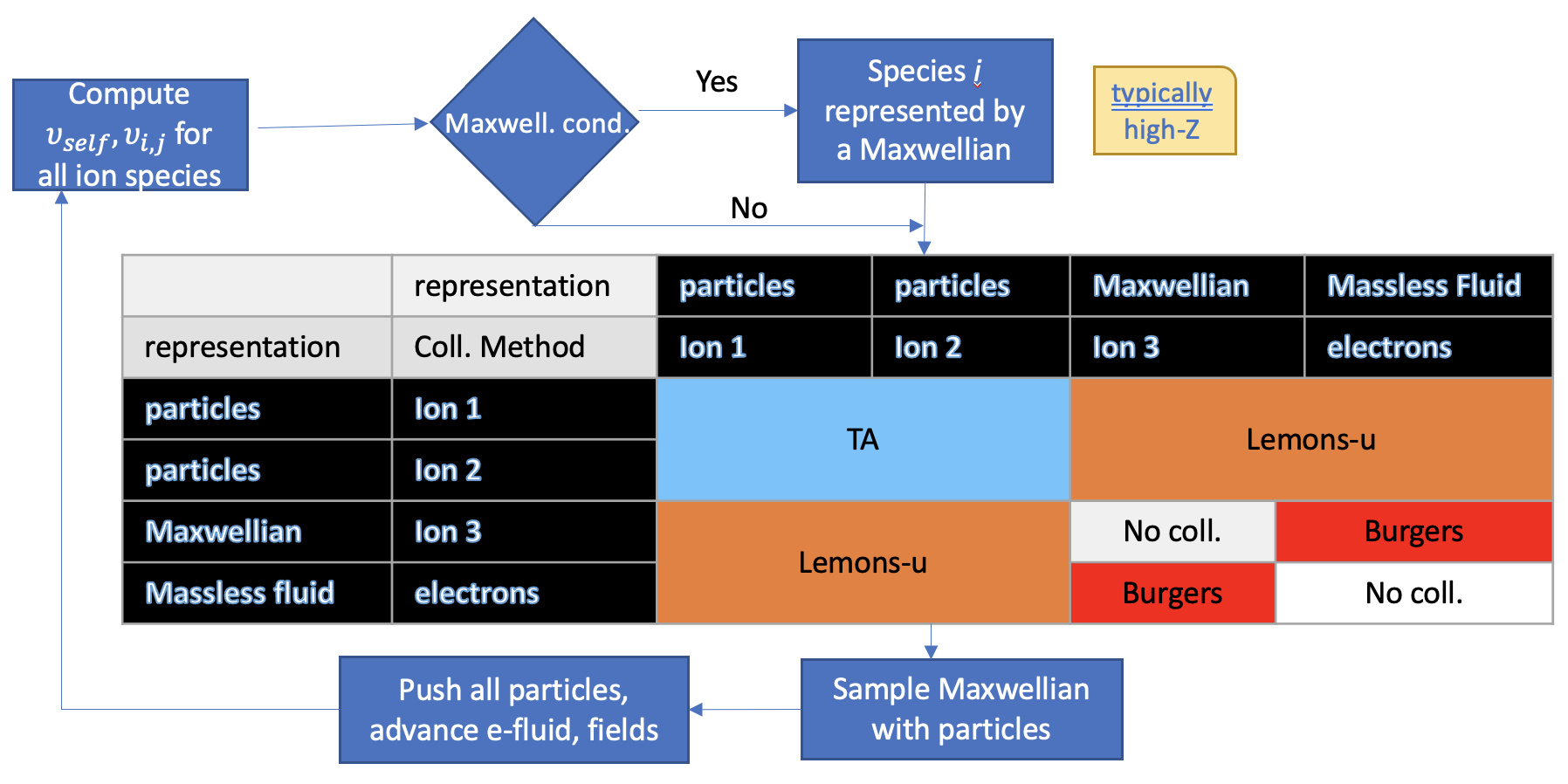
Figure 1: Flowchart of an HMMC step coupled with other parts of the hybrid model. For the purposes of illustration, the flowchart assumes two kinetic ion species, a Maxwellian ion species, and a massless electron fluid species.

Figure 1 illustrates the operation of the hybrid particle-Maxwellian collisions model, which comprises three types of collisions: Maxwellian-Maxwellian, particle-Maxwellian, and particle-particle. This algorithm can deal with any plasma collisionality, but is particularly advantageous for plasma systems featuring a combination of weakly and strongly collisional species, where one or more species can be effectively represented by Maxwellian distribution functions. The criterion for selecting the Maxwellian approximation is the magnitude of the self-collision frequency becoming stiff, i.e. $\nu_{self}\Delta t>1$, except when the number of particles in that cell is too low for a Maxwellian reconstruction (we typically use four particles as the threshold), in which case we revert back to TA.

The algorithm functions as follows: it iterates through species pairs for collision events. For each pair, the appropriate collision model is selected from the three considered in this study. If a species is deemed to follow a Maxwellian distribution, the advancement of its first five moments due to collisions is determined. Upon completion of all collision pairs, an additional step samples particles from the post-collision Maxwellian distributions. These particle samples are subsequently utilized for the Vlasov transport step.

As described in the previous section, conservation of mass, momentum, and energy are strictly enforced for each collisional process considered in the algorithm. As a result, the total mass, momentum, and energy conservation is conserved exactly (in practice, to numerical round-off error) after all collisional processes have been performed.

3 Numerical experiments

We have implemented the HMMC algorithm in C++, leveraging the parallelization strategies offered by the Cabana [47] and Kokkos [48] libraries. We conduct a comprehensive evaluation of our proposed HMMC method and its components with a series of numerical tests intended to highlight its advantages, capabilities, and potential advancements over existing approaches. Our numerical experiments start with a two-species relaxation test intended to validate the extended TA model with non-equal weights introduced earlier in this study (see Sec. 2.3).

We continue with particle-Maxwellian collisions, where we compare the standard Lemons method [7] with the enhanced one proposed in this study, with a focus on particles exhibiting low relative and thermal speeds. Given their prolonged collision times with the Maxwellian distribution, these low-relative speed particles are expected to undergo significant scattering angles, leading to isotropic scattering. This behavior necessitates a distinct modeling approach from that for particles with higher relative speed.

Subsequently, we test the full hybrid method (i.e., considering all possible collisional processes) to a challenging relaxation problem involving He-C-Au-e interactions. This scenario, which is inspired by conditions usually encountered in ICF hohlraums, includes realistic high-mass-ratios and high-Z species in a stiff and self-consistently coupled system relaxing collisionally.

Finally, we consider the coupling of our HMMC approach with a fully self-consistent PIC-ion/fluid-electron model to simulate a 1D plasma interpenetration problem in typical ICF hohlraum conditions, inspired by recent experiments conducted by Le Pape et al. [49], demonstrating the ability of the HMMC method to capture transport in realistic plasma scenarios.

3.1 Overview of the iFP Vlasov-Fokker-Planck Code

For verification of the HMMC algorithm, we compare our results against simulations obtained with the plasma kinetic code iFP [26, 27, 28]. iFP is an Eulerian Vlasov-Fokker-Planck code that solves for the ion distribution functions on a phase-space grid. The iFP code is one-dimensional in physical space and two-dimensional in velocity-space ($v_{\parallel},v_{\bot}$), a valid configuration under a 1D electrostatic approximation without loss of generality. Electrons are modeled as quasineutral and ambipolar fluid with zero charge and current density, possessing their own temperature. iFP solves for the fully Landau-Fokker-Planck collisional model, using the Rosenbluth formulation for optimal performance. To further reduce computational cost, iFP employs mesh adaptivity in the physical space through a mesh-motion scheme that optimizes the grid to resolve features such as gradients of the moment quantities. Additionally, iFP utilizes a mesh-transformation strategy in velocity-space, where each species’ velocity-space mesh is shifted based on its bulk velocity and scaled according to its thermal speed. iFP has been designed to conserve mass, momentum, and energy exactly (in practice, to nonlinear tolerance) for both Vlasov and collision-operator components, making it uniquely suited for verification purposes. In the tests that follow, unless otherwise specified, iFP employs a velocity-space grid resolution $[N_{v_{\parallel}},N_{v_{\bot}}]=[256,128]$, with domain extent [$v_{\parallel,\min},v_{\parallel,\max}]=[-7v_{th},7v_{th}]$, [$v_{\bot,\min},v_{\bot,\max}]=[0,7v_{th}]$.

3.2 Unequal-weight MC algorithm

To assess the unequal-particle-weight TA method, we follow Ref. [36] and consider a two-species relaxation problem with initial conditions outlined in Table 1.

Table 1: Initial conditions for the two-species relaxation test. The problem is set to have a density ratio of 10.

	species 1	species 2
mass	1	20.0
Z number	1	20.0
density	0.1	1.0
drift velocity	0.0	10.0
thermal velocity (x)	1.0	0.2236
thermal velocity (y)	1.0	0.2236
thermal velocity (z)	1.0	0.2236

The results are presented in Figure 2. Four runs with varying numbers of particles are conducted: $N_{1}=N_{2}=300$, $N_{1}=10^{4}$ and $N_{2}=10^{3}$, $N_{1}=N_{2}=10^{4}$, and $N_{1}=10^{4}$ and $N_{2}=10^{5}$. Given a density ratio between the two species $n_{2}/n_{1}=10$, the weight ratios for the four particle-number configurations are $w_{2}/w_{1}=10,100,10,1$, respectively. The run with $N_{1}=N_{2}=300$ is the noisiest, as expected. However, there is excellent agreement between runs with different particle weights. Figure 3 shows the history of the conservation properties of the various particle weighting numerical experiments. For all cases, the noise level of the conservation of energy and momentum is at or better than $10^{-10}$, improving with the number of sample particles, as expected. If the conservation error is normalized to the number of particles, the average error is $\lesssim 10^{-14}$, of order the double-precision round-off error.

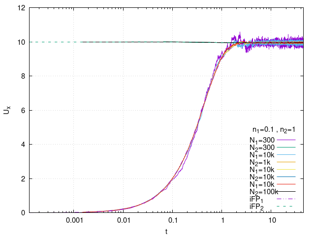
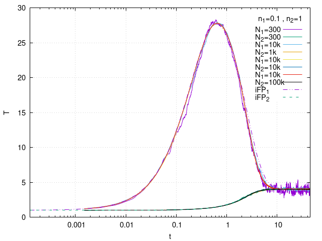
Figure 2: Comparison of the two-species relaxation test results using the TA algorithm with non-equal particle weights for various particle-number choices and with iFP. All simulations are in excellent agreement.

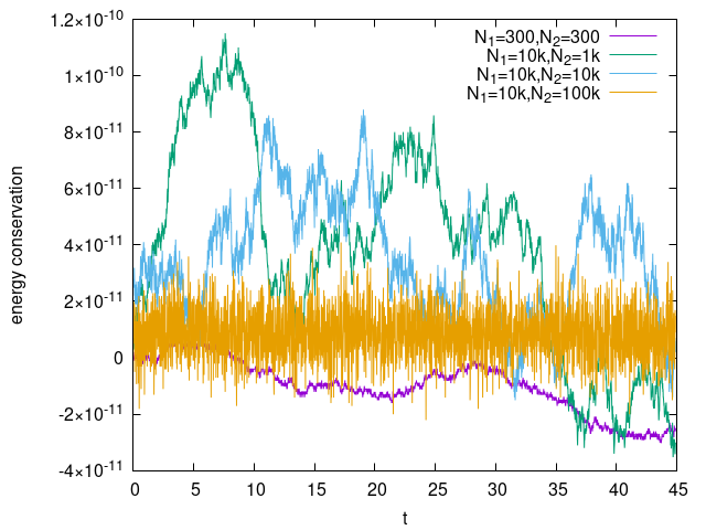
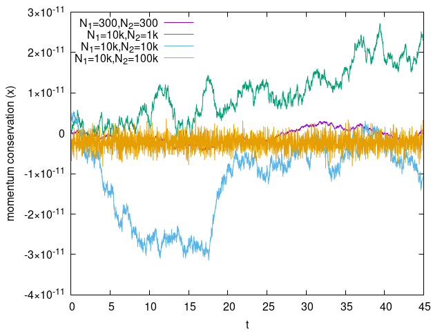
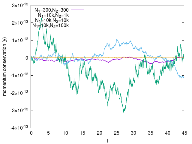
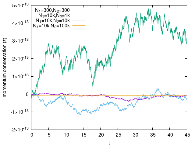
Figure 3: Conservation properties of non-equal weight TA method. Errors (relative to the initial values) of conservation of energy (top-left) and x-momentum (top-right) are at the $10^{-11}$ level. Errors in the other two momenta (y and z directions, which have zero initial momentum) are conserved to $<10^{-13}$.

3.3 Improved particle-Maxwellian (fluid) Lemons algorithm

In Ref. [7], the Lemons method (also known as “particle-moment” method) was tested with two test problems: a single-component plasma, and two equal density, equal mass Maxwellian components with different initial temperatures. In the reference, they were able to use a timestep about 10% of the relaxation time, which is much larger than that allowed by the classic TA method. Such performance gain was attributed to the fact that the method deals with collisions of test particles with the target Maxwellian distribution instead of colliding individual particles. However, the failure mode of the original method discussed in Sec. 2.2 cannot be detected with the two tests used in the reference.

Here, we compare the original Lemons method, our proposed improved version, and the classic TA method using a relaxation problem of a homogeneous particle-ion/fluid-electron plasma (i.e., with disparate masses). In the test, for the ion species we take $m_{i}=1$, $q_{i}=1$, $v_{i0}=0.5$, and $T_{i0}=1$. The electron mass is 0.01, the electron charge is $q_{e}=-1$, and the electron temperature is $T_{e0}=545$. The ions have an average drift velocity of 0.5, while electrons are stationary. Both species are initialized as Maxwellians. We employ $N_{p}=1000$ for Lemons, and $N_{p}=10,000$ for TA. The results are shown in Fig. 4. Clearly, the original Lemons method fails to capture the right behavior of the temperature relaxation, and features significant fluctuations due to enhanced particle noise. The improved Lemons method not only agrees very well with TA, but uses 10 times fewer particles and 100 times larger timesteps. The overall efficiency gain of Lemons vs. TA for this case is about $10^{3}$.

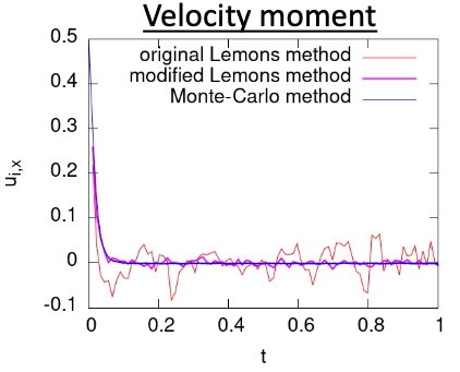
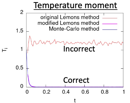
Figure 4: Comparison of two-species (ion, electrons) momentum and temperature relaxation simulations using Lemons, improved Lemons, and TA methods. Incorrect results are obtained with the original Lemons method using $\Delta t=0.014$. The improved Lemons method produces correct results using the same timestep, as assessed by comparison with a temporally resolved TA simulation using $\Delta t=1.4\times 10^{-4}$.

3.4 Full HMMC algorithm (0D)

We verify next the full HMMC algorithm self-consistently with a 0D multi-species system comprising four species: Helium, Carbon, Gold, and electrons. Simulation initial conditions are as described in Table 2. In this setup, the electron and Gold species are described by a fluid model, while the rest are treated as particles. The simulation incorporates all collisional interactions among species.

In this system, Gold self-collisions exhibit the fastest timescales, owing to its high atomic number ($\nu\propto Z^{4}$). Specifically, the Gold self-collision frequency is approximately one to two orders of magnitude faster than any other collision timescales in the system. This poses a stiffness challenge if resolved temporally in the simulation, as required by the TA method for accuracy [5]. To avoid this, we represent the Gold species as a Maxwellian distribution, while the other two ion species are treated with particles.

Figure 5 presents the results of momentum and energy relaxation for the four species from the hybrid model, demonstrating very good agreement with iFP. Figure 6 demonstrates strict conservation of momentum and energy of HMMC to near double precision when the error is normalized by the number of particles. In terms of efficiency, for this simulation HMMC is about 100$\times$ faster than the TA method when it is resolving the fastest collisional time scales (assuming $\nu\Delta t_{TA}=0.01$, as needed for accuracy [5]).

Table 2: Initial condition for the 4-species relaxation. The problem is set to have a density ratio of 10.

	Helium	Carbon	Gold	e-fluid
mass	4	12	197	1/1837
Z number	2	6	30	1
density	1.0	0.1	1.0	32.6
drift velocity	0.0	0.6462	0.9693	0.9329
thermal velocity (x)	1.5811	1.5275	0.07125	42.8602
thermal velocity (y)	1.5811	1.5275	0.07125	42.8602
thermal velocity (z)	1.5811	1.5275	0.07125	42.8602

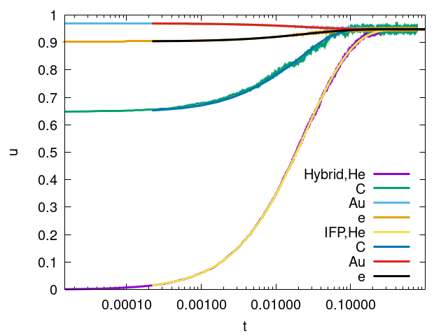
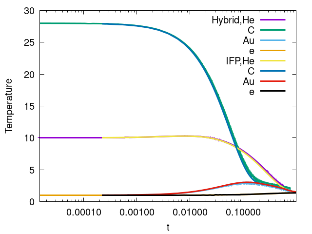
Figure 5: Comparison of hybrid collision algorithm with the iFP for a four-species relaxation problem. Here the Gold species is represented by a drift Maxwellian distribution. The number of particles used for the kinetic species He and C are $10^{5}$ and $10^{4}$, respectively.

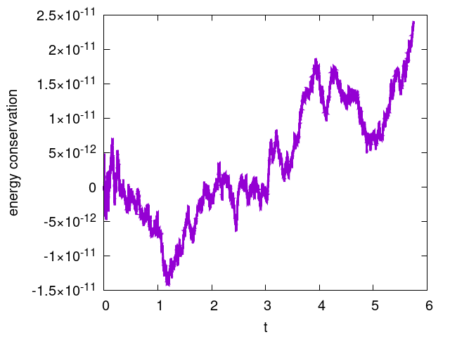
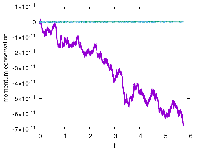
Figure 6: Conservation properties of HMMC algorithm. Errors of conservation of energy (left) and the x component of momentum (right, magenta) is realized to to $10^{-11}$ level. The y and z components of momentum (cyan) are conserved to $10^{-14}$ level.

3.5 A 1D multispecies plasma interpenetration problem in a hohlraum-like environment

Our final demonstration tests the collective behavior of multi-species relaxation and transport in a plasma interpenetration problem inspired by the recent experiments of Le Pape et. al. [49]. In this experiment, a high-density carbon puck (density $3.45\mathrm{g/cc}$, radius $600\mu\mathrm{m}$) is centered within a circular gold band (density $19.3\mathrm{g/cc}$, inner radius $1600\mu\mathrm{m}$, thickness $25\mu\mathrm{m}$), with a low-density helium gas fill ($0.15\mathrm{mg/cc}$) present between. The carbon and inner gold surfaces are subjected to a laser-driven ablation via $351\mathrm{nm}$ laser light, which is intended to simulate the plasma environment within an indirect-drive inertial confinement fusion (ICF) hohlraum. The carbon and gold produce coronal plasma blowoff which counterpropagates and collides in the middle of the domain, compressing the helium fill. This is a very stringent numerical test due to the scale separation present, and the sensitivity of the species interpenetration and temperature transport to the accuracy of the collisional process.

Here, we model a planar-geometry surrogate of the Le Pape experiment with static boundary conditions (non-moving, non-time-dependent), which is intended to replicate the experimental plasma conditions. The initial and boundary conditions are chosen to mimic the plasma state in the coronal blowoff below the critical density, soon after the laser drive starts. We choose representative average ionization states for the ion species to be $Z_{He}=2.0$, $Z_{C}=6.0$, $Z_{Au}=32.0$. The boundaries are located at $0\mu\mathrm{m}$ (carbon) and $1000\mu\mathrm{m}$ (gold). The initial/boundary parameters are chosen for carbon, gold, and helium to be $n_{C,0}=2\times 10{}^{26}\mathrm{m}^{-3}$, $T_{C,0}=2\mathrm{keV}$,$u_{\parallel,C,0}=250\mathrm{km/s}$, $n_{Au,0}=2\times 10{}^{26}\mathrm{m}^{-3}$, $T_{Au,0}=0.75\mathrm{keV}$, $u_{\parallel,Au,0}=-1.5\mathrm{km/s}$, $n_{He,0}=2.25\times 10{}^{25}\mathrm{m}^{-3}$, $T_{He,0}=26.83\mathrm{eV}$, and $u_{\parallel,He,0}=0\mathrm{km/s}$. The carbon and gold number density initial spatial profiles are computed using a hyperbolic cosine switch,

$$n_{C,Au}(x)=n_{C,Au,0}\frac{1}{\left[\cosh\left(\frac{x-x_{C,Au,0}}{\lambda}\right)\right]^{2}},$$ (58)

with $\lambda=62.5\mu\mathrm{m}$, $x_{C,0}=0\mu\mathrm{m}$ is left boundary for $C$ and $x_{C,0}=1000\mu\mathrm{m}$ right boundary for $Au$. Note that for the iFP simulations, zero particle density is not possible, so a number density floor of $4.2\times 10^{20}\mathrm{m}^{-3}$ is used to approximate near-vacuum conditions. The initial spatial profile of temperature for carbon and gold and density for helium taken to be uniform (equal to the parameters $T_{C,0}$, $T_{Au,0}$, $n_{He,0}$, respectively). For a collisionally quiescent initial condition, the initial spatial temperature profile of the helium and the electrons is set to be:

$$T_{e,He}(x)=\frac{T_{He,0}Z_{He}n_{He}+T_{C,0}Z_{C}n_{C}+T_{Au,0}Z_{Au}n_{Au}}{Z_{He}n_{He}+Z_{C}n_{C}+Z_{Au}n_{Au}},$$ (59)

and the initial bulk velocity profiles of all ion species are computed as:

$$u_{\parallel,C,Au,He}(x)=\frac{u_{\parallel,He,0}n_{He}+u_{\parallel,C,0}n_{C}+u_{\parallel,Au,0}n_{Au}}{n_{He}+n_{C}+n_{Au}}.$$ (60)

The electrons are solved as a quasineutral/ambipolar fluid, thus their number density and bulk velocity are determined at all times from the conditions:

$$n_{e} =\sum_{\alpha\in[C,Au,He]}Z_{\alpha}n_{\alpha},$$ (61)

$$u_{\parallel,e} =\frac{\sum_{\alpha\in[C,Au,He]}Z_{\alpha}n_{\alpha}u_{\parallel,\alpha}}{n_{e}}.$$

Our HMMC collisional algorithm has been implemented in a 1D hybrid particle-in-cell code solving the exact same set of equations as iFP [26]. The hybrid particle in cell code is operator-split, performing a collision timestep first (using HMMC), followed by a standard leap-frog field/particle advance. The average number of particles per cell is 1070, 594, and 594 for the He, C, and Au species, respectively. We employ 64 uniform cells and $\Delta t=0.00234$ ps in the hybrid simulation.

Figure 7 presents a comparison between the HMMC simulation and iFP. We plot the first three moments (density, momentum, and pressure) obtained from the simulations. Despite the different discretizations and timestepping solvers in the two approaches, we observe an overall excellent agreement between them throughout the span of the simulation (0.42 ns, which is a very long time in these types of experiments). The most precise agreement is observed in the density, representing the zeroth moment. However, for higher moments, the agreement remains strong at early times and gradually reveals some minor differences, likely attributable to noise levels in low-density regions arising from the limited number of particles available. Overall, the level of agreement is remarkable between the two simulations, lending credibility to the HMMC approach. The speedup of HMMC vs. TA for this case is $>100\times$ assuming $\nu\Delta t_{TA}=0.01$ to resolve the fastest collisional time scales for accuracy.

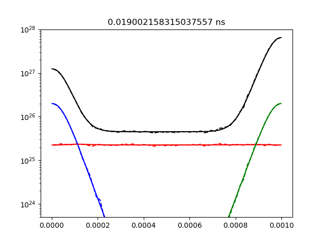
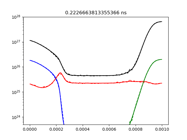
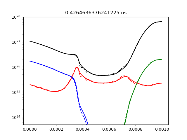
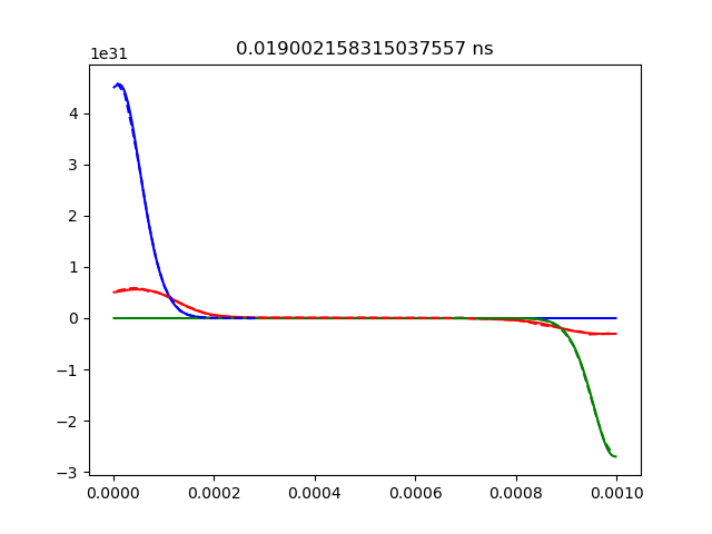
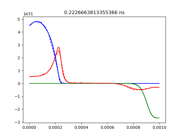
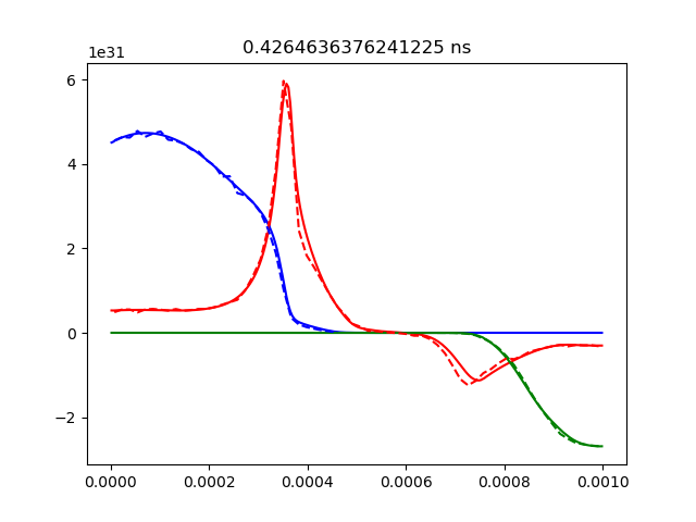
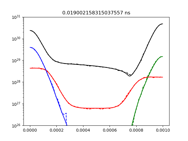
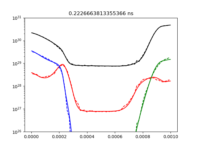
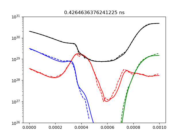
Figure 7: 1D simulation of the plasma interpenetration problem. The solid lines depict results from iFP, while the dashed lines depict the HMMC simulation. Moving from left to right, three different time snapshots are captured. From top to bottom, the three rows display density, momentum, and pressure. In the figure, black is for electrons, green is for gold, blue is for carbon, and red is for helium.

4 Discussion and summary

We have proposed a multiscale algorithm for multispecies particle collisions, HMMC, that is able to improve performance vs. classic MC methods by several orders of magnitude without loss of long-term accuracy. HMMC considers Maxwellians for highly collisional species and particles for moderately or weakly collisional ones, and implements a multitiered collisional strategy comprising particle-particle (with an extended TA algorithm), particle-Maxwellian (with an improved Lemons algorithm), and Maxwellian-Maxwellian (with a five-moment model) interactions. Each collisional interaction is strictly conservative, and as a result the whole algorithm conserves mass, momentum, and energy to numerical round-off. By considering a Maxwellian description for highly collisional species, HMMC removes the stiff self-collision timescale from the process, resulting in significant acceleration vs. classical MC (TA).

We have improved the individual component algorithms in various ways. For TA MC particle-particle collisions, we have extended the algorithm to use variable weights without loss of accuracy. For Lemons particle-Maxwellian collisions, we have fixed a failure mode in the limit of small relative velocities between the particle and the Maxwellian that enables accurate descriptions in arbitrary collisionality regimes while employing larger timesteps. Finally, we have outlined how to couple HMMC with a hybrid kinetic-ion/fluid-electron model, including the form of the collisional sources needed for strict conservation, and the form of the friction force to be applied to the ion species from the interaction with the electron fluid.

We have demonstrated HMMC with challenging relaxation (0D, with both fluid and kinetic species) and transport (1D, with a hybrid kinetic-ion/fluid-electron description) problems, inspired from realistic conditions present in ICF hohlraum environments (which typically feature many plasma species of varying ionization levels, including highly ionized ones that are particularly difficult to treat collisionally due to the $Z^{4}$ scaling of the collision frequency). In all tests, we have verified our implementation against the state-of-the-art hybrid Vlasov-Fokker-Planck code iFP, finding excellent agreement. Our HMMC algorithm has been shown to be one to two orders of magnitude faster for these applications than classical MC without accuracy impact on the simulations, underscoring its effectiveness for plasmas featuring varying collisionality regimes.

References

- [1] P. Helander and D. J. Sigmar, Collisional transport in magnetized plasmas, vol. 4. Cambridge university press, 2005.
- [2] T. Takizuka and H. Abe, “A binary collision model for plasma simulation with a particle code,” Journal of computational physics, vol. 25, no. 3, pp. 205–219, 1977.
- [3] K. Nanbu, “Theory of cumulative small-angle collisions in plasmas,” Physical Review E, vol. 55, no. 4, p. 4642, 1997.
- [4] C. Wang, T. Lin, R. Caflisch, B. I. Cohen, and A. M. Dimits, “Particle simulation of coulomb collisions: Comparing the methods of takizuka & abe and nanbu,” Journal of Computational Physics, vol. 227, no. 9, pp. 4308–4329, 2008.
- [5] B. I. Cohen, A. M. Dimits, A. Friedman, and R. E. Caflisch, “Time-step considerations in particle simulation algorithms for coulomb collisions in plasmas,” IEEE transactions on plasma science, vol. 38, no. 9, pp. 2394–2406, 2010.
- [6] M. Sherlock, “A monte-carlo method for coulomb collisions in hybrid plasma models,” Journal of Computational Physics, vol. 227, no. 4, pp. 2286–2292, 2008.
- [7] D. S. Lemons, D. Winske, W. Daughton, and B. Albright, “Small-angle coulomb collision model for particle-in-cell simulations,” Journal of Computational Physics, vol. 228, no. 5, pp. 1391–1403, 2009.
- [8] D. P. Higginson and A. J. Link, “A cartesian-diffusion langevin method for hybrid kinetic-fluid coulomb scattering in particle-in-cell plasma simulations,” Journal of Computational Physics, vol. 457, p. 110935, 2022.
- [9] D. J. Larson, “A coulomb collision model for pic plasma simulation,” Journal of Computational Physics, vol. 188, no. 1, pp. 123–138, 2003.
- [10] R. Caflisch, C. Wang, G. Dimarco, B. Cohen, and A. Dimits, “A hybrid method for accelerated simulation of coulomb collisions in a plasma,” Multiscale Modeling & Simulation, vol. 7, no. 2, pp. 865–887, 2008.
- [11] L. F. Ricketson, M. S. Rosin, R. E. Caflisch, and A. M. Dimits, “An entropy based thermalization scheme for hybrid simulations of coulomb collisions,” Journal of Computational Physics, vol. 273, pp. 77–99, 2014.
- [12] R. Caflisch, “Accelerated simulation methods for plasma kinetics,” in AIP Conference Proceedings, vol. 1786, AIP Publishing, 2016.
- [13] M. S. Rosin, L. F. Ricketson, A. M. Dimits, R. E. Caflisch, and B. I. Cohen, “Multilevel monte carlo simulation of coulomb collisions,” Journal of Computational Physics, vol. 274, pp. 140–157, 2014.
- [14] J. A. Carrillo, J. Hu, L. Wang, and J. Wu, “A particle method for the homogeneous landau equation,” Journal of Computational Physics: X, vol. 7, p. 100066, 2020.
- [15] J. A. Carrillo, S. Jin, and Y. Tang, “Random batch particle methods for the homogeneous landau equation,” arXiv preprint arXiv:2110.06430, 2021.
- [16] E. Hirvijoki, “Structure-preserving marker-particle discretizations of coulomb collisions for particle-in-cell codes,” Plasma Physics and Controlled Fusion, vol. 63, no. 4, p. 044003, 2021.
- [17] J. A. Carrillo, M. G. Delgadino, and J. S. Wu, “Convergence of a particle method for a regularized spatially homogeneous landau equation,” Mathematical Models and Methods in Applied Sciences, vol. 33, no. 05, pp. 971–1008, 2023.
- [18] R. Bailo, J. A. Carrillo, and J. Hu, “The collisional particle-in-cell method for the vlasov-maxwell-landau equations,” arXiv preprint arXiv:2401.01689, 2024.
- [19] W. T. Taitano, L. Chacón, A. Simakov, and K. Molvig, “A mass, momentum, and energy conserving, fully implicit, scalable algorithm for the multi-dimensional, multi-species rosenbluth–fokker–planck equation,” Journal of Computational Physics, vol. 297, pp. 357–380, 2015.
- [20] E. Yoon and C. Chang, “A fokker-planck-landau collision equation solver on two-dimensional velocity grid and its application to particle-in-cell simulation,” Physics of Plasmas, vol. 21, no. 3, 2014.
- [21] M. F. Adams, E. Hirvijoki, M. G. Knepley, J. Brown, T. Isaac, and R. Mills, “Landau collision integral solver with adaptive mesh refinement on emerging architectures,” SIAM Journal on Scientific Computing, vol. 39, no. 6, pp. C452–C465, 2017.
- [22] M. F. Adams, D. P. Brennan, M. G. Knepley, and P. Wang, “Landau collision operator in the cuda programming model applied to thermal quench plasmas,” in 2022 IEEE International Parallel and Distributed Processing Symposium (IPDPS), pp. 115–123, IEEE, 2022.
- [23] R. Hager, E. Yoon, S. Ku, E. F. D’Azevedo, P. H. Worley, and C.-S. Chang, “A fully non-linear multi-species fokker–planck–landau collision operator for simulation of fusion plasma,” Journal of Computational Physics, vol. 315, pp. 644–660, 2016.
- [24] E. Hirvijoki and M. F. Adams, “Conservative discretization of the landau collision integral,” Physics of Plasmas, vol. 24, no. 3, 2017.
- [25] W. T. Taitano, L. Chacon, and A. N. Simakov, “An adaptive, conservative 0d-2v multispecies rosenbluth–fokker–planck solver for arbitrarily disparate mass and temperature regimes,” Journal of Computational Physics, vol. 318, pp. 391–420, 2016.
- [26] W. T. Taitano, L. Chacon, and A. N. Simakov, “An adaptive, implicit, conservative, 1d-2v multi-species vlasov–fokker–planck multi-scale solver in planar geometry,” Journal of Computational Physics, vol. 365, pp. 173–205, 2018.
- [27] W. T. Taitano, B. D. Keenan, L. Chacón, S. E. Anderson, H. R. Hammer, and A. N. Simakov, “An eulerian Vlasov-Fokker-Planck algorithm for spherical implosion simulations of inertial confinement fusion capsules,” Computer Physics Communications, vol. 263, p. 107861, 2021.
- [28] W. T. Taitano, L. Chacón, A. N. Simakov, and S. E. Anderson, “A conservative phase-space moving-grid strategy for a 1D-2V Vlasov-Fokker-Planck Equation,” Computer Physics Communications, vol. 258, p. 107547, mar 2021.
- [29] J. Denavit, “Numerical simulation of plasmas with periodic smoothing in phase space,” Journal of Computational Physics, vol. 9, no. 1, pp. 75–98, 1972.
- [30] A. Mollén, M. F. Adams, M. G. Knepley, R. Hager, and C.-S. Chang, “Implementation of higher-order velocity mapping between marker particles and grid in the particle-in-cell code xgc,” Journal of Plasma Physics, vol. 87, no. 2, p. 905870229, 2021.
- [31] J. M. Burgers, Flow equations for composite gases, vol. 108. Academic Press New York, 1969.
- [32] M. M. Echim, J. Lemaire, and Ø. Lie-Svendsen, “A review on solar wind modeling: Kinetic and fluid aspects,” Surveys in geophysics, vol. 32, no. 1, pp. 1–70, 2011.
- [33] R. H. Miller and M. R. Combi, “A coulomb collision algorithm for weighted particle simulations,” Geophysical research letters, vol. 21, no. 16, pp. 1735–1738, 1994.
- [34] K. Nanbu and S. Yonemura, “Weighted particles in coulomb collision simulations based on the theory of a cumulative scattering angle,” Journal of Computational Physics, vol. 145, no. 2, pp. 639–654, 1998.
- [35] Y. Sentoku and A. J. Kemp, “Numerical methods for particle simulations at extreme densities and temperatures: Weighted particles, relativistic collisions and reduced currents,” Journal of computational Physics, vol. 227, no. 14, pp. 6846–6861, 2008.
- [36] D. P. Higginson, I. Holod, and A. Link, “A corrected method for coulomb scattering in arbitrarily weighted particle-in-cell plasma simulations,” Journal of Computational Physics, vol. 413, p. 109450, 2020.
- [37] R. Shanny, J. M. Dawson, and J. M. Greene, “One-dimensional model of a lorentz plasma,” The Physics of Fluids, vol. 10, no. 6, pp. 1281–1287, 1967.
- [38] A. Tanaka, K. Ibano, T. Takizuka, and Y. Ueda, “A coulomb collision model for weighted particle simulations with energy and momentum conservation,” Contributions to Plasma Physics, vol. 58, no. 6-8, pp. 451–456, 2018.
- [39] D. Winske, H. Karimabadi, A. Y. Le, N. N. Omidi, V. Roytershteyn, and A. J. Stanier, “Hybrid-kinetic approach: Massless electrons,” in Space and Astrophysical Plasma Simulation: Methods, Algorithms, and Applications, pp. 63–91, Springer, 2023.
- [40] L. Spitzer, Physics of fully ionized gases. Courier Corporation, 2006.
- [41] G. Milstein, “Approximate integration of stochastic differential equations,” Theory of Probability & Its Applications, vol. 19, no. 3, pp. 557–562, 1975.
- [42] B. Trubnikov, “Particle interactions in a fully ionized plasma,” Rev. Plasma Phys., vol. 1, 1965.
- [43] A. Stanier, L. Chacón, and G. Chen, “A fully implicit, conservative, non-linear, electromagnetic hybrid particle-ion/fluid-electron algorithm,” Journal of Computational Physics, vol. 376, pp. 597–616, 2019.
- [44] S. Braginskii, “Transport phenomena in a completely ionized two-temperature plasma,” Sov. Phys. JETP, vol. 6, no. 33, pp. 358–369, 1958.
- [45] A. N. Simakov and K. Molvig, “Electron transport in a collisional plasma with multiple ion species,” Physics of Plasmas, vol. 21, no. 2, 2014.
- [46] A. Le, A. Stanier, L. Yin, B. Wetherton, B. Keenan, and B. Albright, “Hybrid-vpic: An open-source kinetic/fluid hybrid particle-in-cell code,” Physics of Plasmas, vol. 30, no. 6, 2023.
- [47] S. M. Mniszewski, J. Belak, J.-L. Fattebert, C. F. Negre, S. R. Slattery, A. A. Adedoyin, R. F. Bird, C. Chang, G. Chen, S. Ethier, et al., “Enabling particle applications for exascale computing platforms,” The International Journal of High Performance Computing Applications, vol. 35, no. 6, pp. 572–597, 2021.
- [48] H. C. Edwards, C. R. Trott, and D. Sunderland, “Kokkos: Enabling manycore performance portability through polymorphic memory access patterns,” Journal of parallel and distributed computing, vol. 74, no. 12, pp. 3202–3216, 2014.
- [49] S. Le Pape, L. Divol, G. Huser, J. Katz, A. Kemp, J. S. Ross, R. Wallace, and S. Wilks, “Plasma Collision in a Gas Atmosphere,” Physical Review Letters, vol. 124, no. 2, p. 25003, 2020.