An EM Body Model for Device-Free Localization with Multiple Antenna Receivers: A First Study

Abstract

Device-Free Localization (DFL) employs passive radio techniques capable to detect and locate people without imposing them to wear any electronic device. By exploiting the Integrated Sensing and Communication paradigm, DFL networks employ Radio Frequency (RF) nodes to measure the excess attenuation introduced by the subjects (i.e., human bodies) moving inside the monitored area, and to estimate their positions and movements. Physical, statistical, and ElectroMagnetic (EM) models have been proposed in the literature to estimate the body positions according to the RF signals collected by the nodes. These body models usually employ a single-antenna processing for localization purposes. However, the availability of low-cost multi-antenna devices such as those used for WLAN (Wireless Local Area Network) applications and the timely development of array-based body models, allow us to employ array-based processing techniques in DFL networks. By exploiting a suitable array-capable EM body model, this paper proposes an array-based framework to improve people sensing and localization. In particular, some simulations are proposed and discussed to compare the model results in both single- and multi-antenna scenarios. The proposed framework paves the way for a wider use of multi-antenna devices (e.g., those employed in current IEEE 802.11ac/ax/be and forthcoming IEEE 802.11be networks) and novel beamforming algorithms for DFL scenarios.

I Introduction

Device-Free Localization (DFL), also known as Passive Radio Localization (PRL), is an opportunistic set of methods capable to detect, locate, and track people in a monitored area covered by ambient Radio Frequency (RF) signals. By exploiting the Integrated Sensing and Communication paradigm [1], DFL systems are able to transform each RF node of the wireless network covering the monitored area into a virtual sensor able perform sensing operations as well.

For instance, the RF signals emitted for communication purposes by a wireless network over the monitored area, can be usefully employed to estimate people location and status information from the received ElectroMagnetic (EM) field. In fact, it is well known that the presence, and the movements, of people, or objects, generically indicated as targets, induce modifications and alterations of the EM field [2] collected by each wireless device of the communication network. These perturbations not only impair the radio channel, but can be also measured and processed to estimate information about the presence, location, and status (e.g., posture, movements, size, etc.) of the targets [3].

Body models for DFL applications have been mostly evaluated for single-antenna DFL systems for both single-target [4, 5, 6, 7] and multi-targets [8] scenarios. These models have been applied to different radio channel measurements, such as Channel State Information (CSI), Received Signal Strength (RSS), Angles of Arrival (AoA) and Time of Flight (ToF) [1], and processed by different methods such as radio imaging [4], Bayesian tracking [9], fingerprinting methods [1], Compressive Sensing algorithms [10], and Machine Learning/Deep Learning (ML/DL) systems [3, 11], to evaluate the connection between targets location and the corresponding measured perturbations.

At the same time, the wide diffusion of multi-antenna WLAN devices (e.g., WiFi devices built according to the IEEE 802.11n/ac/ax standards and the forthcoming IEEE 802.11be one), and the concomitant availability of CSI extraction tools [12, 13, 14], have stimulated the research activities with the adoption of multi-antenna CSI-based processing systems for DFL applications [15, 16, 17].

Unfortunately, only a few body models deal with antenna arrays [18, 20, 19] since almost all array-based DFL systems hold the attention on the processing steps instead of focusing on the body model. However, reference [18] employs a very simple propagation model while [19] exploiting a computational-intensive Ray Tracing (RT) approach. Of course, EM simulators can be also used, but they are too complex to be of practical use for on-line DFL systems as based on RT techniques, uniform theory of diffraction (UTD), or full-wave methods as shown in [8] (and included references).

The paper extends the physical-statistical array-based model proposed by the authors in [20] to predict the body-induced propagation losses using WLAN nodes equipped with multiple antennas at the receiver node. The body model is then used, in conjunction with array processing techniques, to focus on the AoA and the position of the target. The paper is organized as follows: in Sect. II, the array-based electromagnetic body model for applications in multi-antennas DFL systems is briefly recalled and discussed. Sect. III proposes the array-based processing tools for DFL applications while Sect. IV presents some preliminary simulation results comparing the array-based model with the single-antenna one. Finally, in Sect. V, we draw some preliminary conclusions and propose future activities.

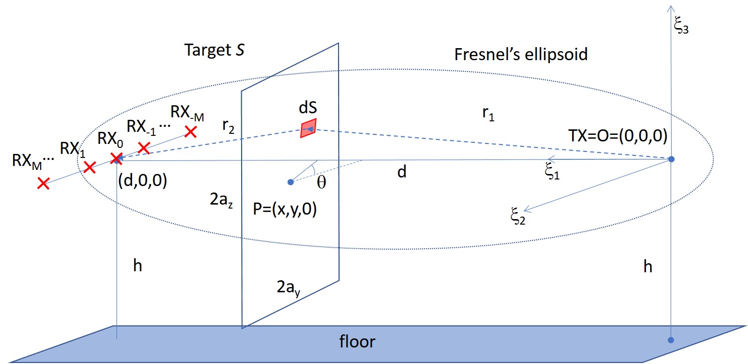
Figure 1: 3-D deployment of the radio link using an ULA-like array of $2M+1$ antennas. The segment where the array is deployed is placed at distance $d=d_{0}$ from the TX and it is orthogonal to the LoS path connecting the $TX$ node with the $RX_{0}$ one.

II EM body model with multiple antenna receiver

In this section we briefly recall the body model proposed in [20] for a single link scenario where an antenna array is used at the receiver while only one transmitter (TX) is used. Fig. 1 shows the layout for an Uniform Linear Array (ULA) of $2M+1$ isotropic receiver antennas RX_m, with$-M\leq m\leq M$ and $M$ an integer, when a single target $S$ is in the monitored area near the radio link.

The 2-D footprint of the 3-D deployment of Fig. 1 is also shown in Fig. 2, where each m-th antenna RX_m of the array is uniformly deployed at mutual distance $d_{a}$ along a segment orthogonal to the Line-of-Sight (LoS) at distance $d=d_{0}$ from the TX and horizontally placed w.r.t. the floor. The central antenna is indicated by the index $m=0$.

Without any loss of generality, we assume here that the floor has no influence on the radio propagation but it only needed to support the standing target. However, if needed, the EM influence of the floor can be easily included as shown in [21]. The target is sketched [7] as a vertical standing absorbing 2-D sheet $S$ of height $2a_{z}$ and traversal size $2a_{y}$ that is rotated of the angle $\theta$ w.r.t. the $\xi_{2}$ axis. Excluding mutual antenna coupling (approximately valid for $d_{a}>\lambda/4$), the electric field $E^{\left(m\right)}$ received by the m-th antenna of the array, is:

$$\begin{array}[]{ll}\frac{E^{\left(m\right)}}{E_{R}^{\left(m\right)}}=&1-j\frac{d_{m}}{\lambda}\intop_{S}\frac{1}{r_{1,m}r_{2,m}}\cdot\\ &\cdot\exp\left\{-j\frac{2\pi}{\lambda}\bigl{(}r_{1,m}+r_{2,m}-d_{m}\bigr{)}\right\}d\xi_{2}\,d\xi_{3},\end{array}$$ (1)

where $E_{R}^{\left(m\right)}$ is the EM field received by the same $RX_{m}$ node in the reference condition i.e. the free-space scenario characterized by the absence of any target in the link area. The term $d_{m}$ indicates the distance of the m-th antenna $RX_{m}$ of the array from the TX while $d_{1,m}$ and $d_{2,m}$ are the distances of the projection point $O_{m}^{{}^{\prime}}$ (of the barycenter $P$ of the 2-D surface $S$) from the TX and $RX_{m}$ nodes. Likewise, $r_{1,m}$ and $r_{2,m}$ are the distances of the generic elementary area $dS$ of the target $S$ from the TX and $RX_{m}$, respectively. In (1), the integration operations are performed over the squared domain $S$ having height $2a_{z}$ and traversal size $2a_{y}$.

Notice that, for $M=0$, equation (1) reduces to the single-antenna case where RX₀ coincides with the RX antenna at distance $d=d_{0}$ from the TX. The excess attenuation [7] measured by the m-th antenna of the array, that is due to the target w.r.t. the free-space scenario, is thus given by $A_{T}^{\left(m\right)}=P_{R}^{\left(m\right)}/P^{\left(m\right)}=\left|E_{R}^{\left(m\right)}/E^{\left(m\right)}\right|^{2}$ where $P_{R}^{\left(m\right)}$ and $P^{\left(m\right)}$ are the m-th received power in without and with a target in the link area, respectively. Usually, the excess attenuation is given in dB as $A_{T,dB}^{\left(m\right)}=10\,\log_{10}\left|E_{R}^{\left(m\right)}/E^{\left(m\right)}\right|^{2}$. It is worth noticing that, for short arrays, the excess attenuation due to the target is almost constant along the receiving antennas as shown in [20].

In free-space conditions, the term $E_{R}^{\left(m\right)}/E_{R}^{\left(0\right)}$ is given by:

$$\begin{array}[]{ll}\frac{E_{R}^{\left(m\right)}}{E_{R}^{\left(0\right)}}=&\frac{d_{0}}{d_{m}}\,\exp\left\{-j\frac{2\pi}{\lambda}\bigl{(}d_{m}-d_{0}\bigr{)}\right\},\end{array}$$ (2)

where $E_{R}^{\left(0\right)}$ is the electric field received by the central antenna of the array of index $m=0$ that is on the LoS at distance $d_{0}$ from the TX. Thus, (1) can be rearranged as:

$$\begin{array}[]{ll}\frac{E^{\left(m\right)}}{E_{R}^{\left(0\right)}}=&\frac{d_{0}}{d_{m}}\,\exp\left\{-j\frac{2\pi}{\lambda}\left(d_{m}-d_{0}\right)\right\}\bigl{[}1-j\frac{d_{m}}{\lambda}\intop_{S}\frac{1}{r_{1,m}r_{2,m}}\cdot\bigr{.}\\ &\bigl{.}\cdot\exp\left\{-j\frac{2\pi}{\lambda}\left(r_{1,m}+r_{2,m}-d_{m}\right)\right\}d\xi_{2}\,d\xi_{3}\bigr{]}.\end{array}$$ (3)

For additional details about the array-based model (3) and its validation with the commercial EM simulator FEKO [22], the interested reader can refer to [20].

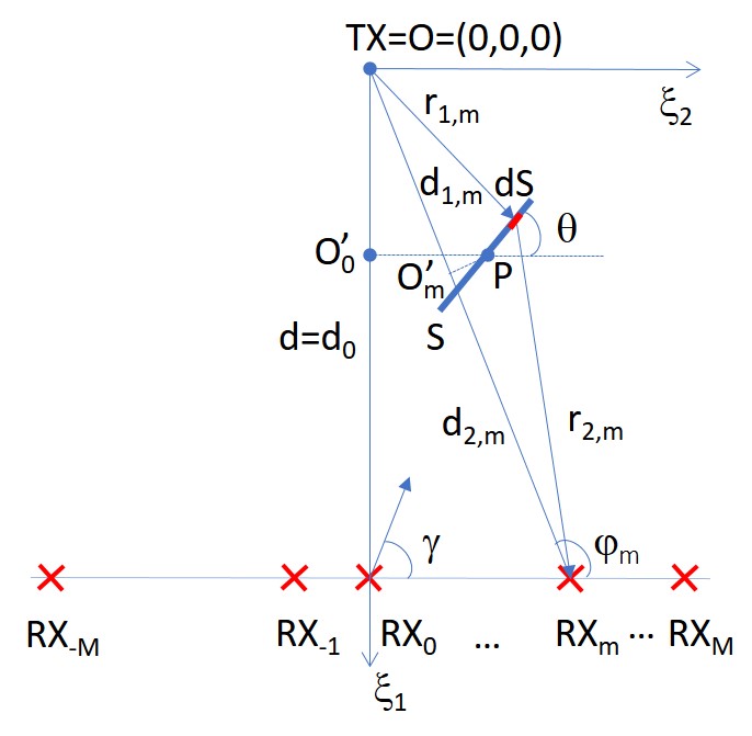
Figure 2: 2-D layout of the radio link of Fig. 1. The point $O_{m}^{{}^{\prime}}$ is the projection of the barycenter $P$ of the target $S$ over the m-th LoS path having length $d_{m}$.

III Array processing with model predictions

In the following sections, we consider the ULA-arranged layout of $2M+1$ antennas of Figs. 1 and 2. Classical array processing, such as conventional beamforming [23], is designed to steer the antenna array in one direction by forming a linear combination of each antenna contribution. Being $\left(\cdot\right)^{T}$ the vector transposition operator, the output of the beamforming processing, considering $2M+1$ antennas and the vector $\mathbf{w}=\left[w_{-M}\,...\,w_{-1}\,w_{0}\,w_{1}\,...\,w_{M}\right]^{T}$ of size $2M+1$ of linear beamforming coefficients, is thus given in general by:

$$y\left(t,\mathcal{S}\right)=\sum_{m=-M}^{+M}w_{m}^{*}\,r_{m}\left(t,\mathcal{S}\right)=\mathbf{w}^{H}\mathbf{r}\left(t,\mathcal{S}\right),$$ (4)

where $\left(\cdot\right)^{*}$ indicates the conjugate operator and $\left(\cdot\right)^{H}$ the Hermitian operator, while $r_{m}\left(t,\mathcal{S}\right)$ is the received EM field at the $RX_{m}$ antenna. The column vector $\mathbf{r}\left(t,\mathcal{S}\right)$ of size $2M+1$, collects all the received electric field terms $\mathbf{r}\left(t,\mathcal{S}\right)=\left[r_{-M}\left(t,\mathcal{S}\right)\,...r_{-1}\left(t,\mathcal{S}\right)\,r_{0}\left(t,\mathcal{S}\right)\,r_{1}\left(t,\mathcal{S}\right)\,...\,r_{M}\left(t,\mathcal{S}\right)\right]^{T}$. Focusing on passive sensing applications, two main scenarios are adopted for processing: the first one refers to the empty environment (i.e., the free-space case, namely $\mathcal{S}=0$) while, in the second scenario, the target $S$ is present in the monitored area ($\mathcal{S}=1$). According to this assumption, the m-th component of the received vector $\mathbf{r}\left(t\right)$ is defined as:

$$r_{m}\left(t,\mathcal{S}\right)=\left\{\begin{array}[]{ll}E_{R}^{\left(m\right)}+n_{m}=E_{R}^{\left(0\right)}\,\frac{E_{R}^{\left(m\right)}}{E_{R}^{\left(0\right)}}+n_{m}&\textrm{if $\mathcal{S}=0$}\\ E^{\left(m\right)}+n_{m}=E_{R}^{\left(0\right)}\,\frac{E_{R}^{\left(m\right)}}{E_{R}^{\left(0\right)}}\,\frac{E^{\left(m\right)}}{E_{R}^{\left(m\right)}}+n_{m}&\textrm{if $\mathcal{S}=1$}\end{array}\right.$$ (5)

where $n_{m}$ is the m-th component of the Additive White Gaussian Noise (AWGN) complex vector $\mathbf{n}\left(t\right)=\left[n_{-M}\left(t\right)\,...n_{-1}\left(t\right)\,n_{0}\left(t\right)\,n_{1}\left(t\right)\,...\,n_{M}\left(t\right)\right]^{T}$ of size $2M+1$, that is assumed to be spatially white with zero mean and covariance $\sigma_{n}^{2}\mathbf{I}$, while $E_{R}^{\left(m\right)}/E_{R}^{\left(0\right)}$ and $E^{\left(m\right)}/E_{R}^{\left(0\right)}$ are given by (2) and (3), respectively. We assume here that the noise distribution does not change according to the presence or absence of the target. For discussions about this topic, the interested reader can refer to [7, 9, 8]. As analyzed in the following sections, different beamforming methods correspond to different choices of the weighting vector $\mathbf{w}$.

Considering the passive radio sensing problem, we are interested in evaluating the power $P_{y}\left(\mathcal{S}\right)$ of the signal $y$ with or without target $S$. This is given by:

$$\begin{array}[]{ll}P_{y}\left(\mathcal{S}\right)&=\mathbb{E}\left[y\left(t,\mathcal{S}\right)\,y^{*}\left(t,\mathcal{S}\right)\right]\\ &=\mathbf{w}^{H}\,\mathbf{R}\left(\mathcal{S}\right)\,\mathbf{w}\end{array}$$ (6)

with $\mathbf{R}\left(\mathcal{S}\right)=\mathbf{R}=\mathbb{E}\left[\mathbf{r}\left(t\right)\,\mathbf{r}^{H}\left(t\right)\right]$ of size $\left(2M+1\right)\times\left(2M+1\right)$, being the autocorrelation matrix of $y\left(t,\mathcal{S}\right).$

III-A Impact of beamforming on body induced attenuation

In what follows, we model the received EM field $r_{m}\left(t,\mathcal{S}\right)$ in (4) using the diffraction model considerations and exploiting the equations (1)-(3) for $\mathcal{S}=1$, and (2) for $\mathcal{S}=0$. For conventional ULA scenarios, that assume planar wavefront propagation, the steering (column) vector $\mathbf{a}=\left[a_{m}\right]$ of size $2M+1$ for the considered array is given by [23]:

$$\begin{array}[]{ll}\mathbf{a}=&\left[\exp\left\{-jM\frac{2\pi}{\lambda}d_{a}\cos\gamma\right\}\right.\\ &\>\exp\left\{-j\left(M-1\right)\frac{2\pi}{\lambda}d_{a}\cos\gamma\right\}\\ &...\>1\>...\\ &\>\exp\left\{+j\left(M-1\right)\frac{2\pi}{\lambda}d_{a}\cos\gamma\right\}\\ &\left.\exp\left\{+jM\frac{2\pi}{\lambda}d_{a}\cos\gamma\right\}\right]^{T},\end{array}$$ (7)

where $\gamma$ is also known as DoA (Direction Of Arrival): this is the direction of propagation of the impinging wavefront w.r.t. the axis of the array, and $d_{a}$ is the inter-element antenna distance. According to (7), it is also $\left|\mathbf{a}\right|^{2}=\mathbf{a}^{H}\mathbf{a}=(2M+1)$. However, due to the fact that most DFL applications are employed in indoor scenarios with relatively short links compared with the usual far-field hypothesis, the planar wavefront assumption no longer holds and the new steering vector is:

$$\begin{array}[]{ll}\mathbf{a}=&\left[\frac{d_{0}}{d_{-M}}\,\exp\left\{-jM\frac{2\pi}{\lambda}d_{a}\frac{\cos\left\{\left(\gamma+\varphi_{-M}\right)/2\right\}}{\cos\left\{\left(\gamma-\varphi_{-M}\right)/2\right\}}\right\}\right.\\ &\frac{d_{0}}{d_{-M+1}}\,\exp\left\{-j\left(M-1\right)\frac{2\pi}{\lambda}d_{a}\frac{\cos\left\{\left(\gamma+\varphi_{-M+1}\right)/2\right\}}{\cos\left\{\left(\gamma-\varphi_{-M+1}\right)/2\right\}}\right\}\\ &\>...\>1...\\ &\frac{d_{0}}{d_{M-1}}\,\exp\left\{+j\left(M-1\right)\frac{2\pi}{\lambda}d_{a}\frac{\cos\left\{\left(\gamma+\varphi_{M-1}\right)/2\right\}}{\cos\left\{\left(\gamma-\varphi_{M-1}\right)/2\right\}}\right\}\\ &\left.\frac{d_{0}}{d_{M}}\,\exp\left\{+jM\frac{2\pi}{\lambda}d_{a}\frac{\cos\left\{\left(\gamma+\varphi_{M}\right)/2\right\}}{\cos\left\{\left(\gamma-\varphi_{M}\right)/2\right\}}\right\}\right]^{T},\end{array}$$ (8)

where the angle $\varphi_{m}$, formed by the LoS of the m-th array antenna with the $\xi_{2}$ axis, also verifies $\forall m=0,\pm 1,...,\pm M$ the following equation $\varphi_{m}=\arccos\left[\left(d_{0}/d_{m}\right)\,\cos\gamma-m\,\left(d_{a}/d_{m}\right)\right]$ with $\varphi_{0}=\gamma$. Moreover, it is also $\left|\mathbf{a}\right|^{2}=\sum_{m=-M}^{M}\left(d_{0}/d_{m}\right)^{2}$. It is easy to check that (8) converges to (7) for planar wavefronts i.e. when $\forall m$, it is $\varphi_{m}=\gamma$. According to (8), the received field $\mathbf{r}\left(t,\mathcal{S}\right)$ is given by:

$$\mathbf{r}\left(t,\mathcal{S}\right)=\left\{\begin{array}[]{ll}E_{R}^{\left(0\right)}\,\mathbf{a}+\mathbf{n}&\textrm{if $\mathcal{S}=0$}\\ E_{R}^{\left(0\right)}\,\textrm{diag$\left(\mathbf{a}\right)$}\,\mathbf{E}_{r}+\mathbf{n}=&\textrm{if $\mathcal{S}=1$,}\end{array}\right.$$ (9)

where the column vector $\mathbf{E}_{r}$ of size $2M+1$ represents the electric field ratio (1) received by the antenna array for $\mathcal{S}=1$. The $m$-th element of this vector is equal to $E^{\left(m\right)}/E_{R}^{\left(m\right)}$.

According to diffraction model of Sect. II, and by rearranging the terms in (9) with (8) and (1), the received field $y\left(t,\mathcal{S}\right)$ after linear beamforming becomes as in eq. (12). Similarly as for the single antenna case [7], the mean excess attenuation $A_{T}$ due to the target $S$ w.r.t. the empty environment, corresponds to the ratio between $P_{y}\left(\mathcal{S}=0\right)$ and $P_{y}\left(\mathcal{S}=1\right)$, by neglecting the noise terms:

$$\begin{array}[]{ll}A_{T}=&\frac{P_{y}\left(\mathcal{S}=0\right)}{P_{y}\left(\mathcal{S}=1\right)}=\frac{\mathbf{w}^{H}\,\mathbf{a}\,\mathbf{a}^{H}\mathbf{w}}{\mathbf{w}^{H}\,\textrm{diag}\left(\mathbf{a}\right)\,\mathbf{R}_{E}\,\textrm{diag}\left(\mathbf{a}^{H}\right)\mathbf{w}}.\end{array}$$ (10)

In particular, $R_{E}$ is the autocorrelation matrix of $E^{\left(m\right)}/E_{R}^{\left(m\right)}$, of size $\left(2M+1\right)\times\left(2M+1\right)$, given by (11).

Equation (10) can be also written as in (13), neglecting the noise terms.

$$\mathbf{R}_{E}=\left[\begin{array}[]{lcr}\left|\frac{E^{\left(-M\right)}}{E_{R}^{\left(-M\right)}}\right|^{2}&...&\frac{E^{\left(-M\right)}}{E_{R}^{\left(-M\right)}}\,\left(\frac{E^{\left(M\right)}}{E_{R}^{\left(M\right)}}\right)^{*}\\ \frac{E^{\left(-M+1\right)}}{E_{R}^{\left(-M+1\right)}}\,\left(\frac{E^{\left(-M\right)}}{E_{R}^{\left(-M\right)}}\right)^{*}&...&\frac{E^{\left(-M+1\right)}}{E_{R}^{\left(-M+1\right)}}\,\left(\frac{E^{\left(M\right)}}{E_{R}^{\left(M\right)}}\right)^{*}\\ ...&...&...\\ \frac{E^{\left(M-1\right)}}{E_{R}^{\left(M-1\right)}}\,\left(\frac{E^{\left(-M\right)}}{E_{R}^{\left(-M\right)}}\right)^{*}&...&\frac{E^{\left(M-1\right)}}{E_{R}^{\left(M-1\right)}}\,\left(\frac{E^{\left(M\right)}}{E_{R}^{\left(M\right)}}\right)^{*}\\ \frac{E^{\left(M\right)}}{E_{R}^{\left(M\right)}}\,\left(\frac{E^{\left(-M\right)}}{E_{R}^{\left(-M\right)}}\right)^{*}&...&\left|\frac{E^{\left(M\right)}}{E_{R}^{\left(M\right)}}\right|^{2}\end{array}\right]$$ (11)

$$y\left(t,\mathcal{S}\right)=\left\{\begin{array}[]{ll}E_{R}^{\left(0\right)}\,\sum_{m=-M}^{+M}w_{m}^{*}\,\frac{d_{0}}{d_{m}}\,\exp\left\{-j\left(M-1\right)\frac{2\pi}{\lambda}d_{a}\frac{\cos\left\{\left(\gamma+\varphi_{m}\right)/2\right\}}{\cos\left\{\left(\gamma-\varphi_{m}\right)/2\right\}}\right\}+n_{m}&\textrm{if $\mathcal{S}=0$}\\ E_{R}^{\left(0\right)}\,\sum_{m=-M}^{+M}w_{m}^{*}\,\frac{E^{\left(m\right)}}{E_{R}^{\left(m\right)}}\,\frac{d_{0}}{d_{m}}\,\exp\left\{-j\left(M-1\right)\frac{2\pi}{\lambda}d_{a}\frac{\cos\left\{\left(\gamma+\varphi_{m}\right)/2\right\}}{\cos\left\{\left(\gamma-\varphi_{m}\right)/2\right\}}\right\}+n_{m}&\textrm{if $\mathcal{S}=1$}\end{array}\right.$$ (12)

$$\begin{array}[]{l}A_{T}=\frac{\left|\sum_{m=-M}^{+M}w_{m}^{*}\,\frac{d_{0}}{d_{m}}\,\exp\left\{-j\left(M-1\right)\frac{2\pi}{\lambda}d_{a}\frac{\cos\left\{\left(\gamma+\varphi_{m}\right)/2\right\}}{\cos\left\{\left(\gamma-\varphi_{m}\right)/2\right\}}\right\}\right|^{2}}{\left|\sum_{m=-M}^{+M}w_{m}^{*}\,\frac{d_{0}}{d_{m}}\,\exp\left\{-j\left(M-1\right)\frac{2\pi}{\lambda}d_{a}\frac{\cos\left\{\left(\gamma+\varphi_{m}\right)/2\right\}}{\cos\left\{\left(\gamma-\varphi_{m}\right)/2\right\}}\right\}\,\left[1-j\frac{d_{m}}{\lambda}\intop_{S}\frac{1}{r_{1,m}r_{2,m}}\exp\left\{-j\frac{2\pi}{\lambda}\bigl{(}r_{1,m}+r_{2,m}-d_{m}\bigr{)}\right\}d\xi_{2}d\xi_{3}\right]\right|^{2}}\end{array}$$ (13)

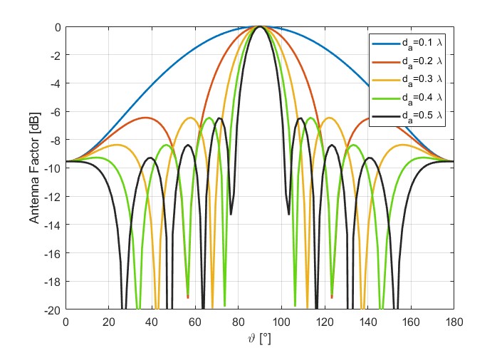
Figure 3: Array factor for an ULA composed by $9$ antennas ($M=4$) uniformly spaced from $0.1\,\lambda$ up to $0.5\,\lambda$.

III-B Array factor analysis

The array factor $F_{a}=\mathbf{w}^{T}\mathbf{a}\left(\gamma\right)$ defines the response of the array as a function of the selected beamforming coefficients $\mathbf{w}$ and of the incident angle $\gamma$ of the steering vector $\mathbf{a}\left(\gamma\right)$ that characterizes the impinging wavefront. For instance, if (7) holds true with the weighting vector $\mathbf{w}$ such that, for all components $w_{m}$, it is $w_{m}=1/(2M+1)$, then the array factor is given by:

$$\begin{array}[]{ll}F_{a}&=\mathbf{w}^{T}\mathbf{a}\left(\gamma\right)=\frac{1}{2M+1}\sum_{m=-M}^{+M}\exp\{{jm\frac{2\pi}{\lambda}d_{a}\cos\gamma}\}\\ &=\frac{1}{2M+1}\cdot\frac{\sin\bigl{\{}\bigl{(}2M+1\bigr{)}\frac{\pi d_{a}}{\lambda}\cos\gamma\bigr{\}}}{\sin\bigl{\{}\frac{\pi d_{a}}{\lambda}\cos\gamma\bigr{\}}}.\end{array}$$ (14)

Fig. 3 shows the modulus of the array factor in dB for an ULA of $9$ antennas ($M=4$) uniformly spaced with $d_{a}$ from $0.1\,\lambda$ up to $0.5\,\lambda$. It is apparent the effect due to the side lobes. The width of the first lobe $\Delta_{BW}$ is given by:

$$\Delta_{BW}=2\left|\arccos\left\{\frac{\lambda}{\left(2M+1\right)d_{a}}\right\}\right|\approx\frac{2\lambda}{\left(2M+1\right)d_{a}},$$ (15)

where the approximation holds for long arrays i.e. for $L=\left(2M+1\right)\,d_{a}\gg\lambda$.

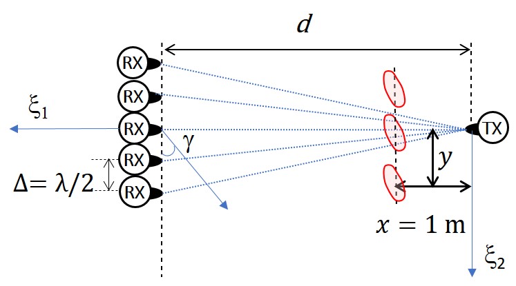
Figure 4: Link layout used for the simulations: the antenna array is composed by 5 antennas ($M=2$) while the target $S$, with size $a_{z}=0.9$ m and $a_{y}=0.275$ m, is placed in different positions along the line having distance $x=1$ m from the TX.

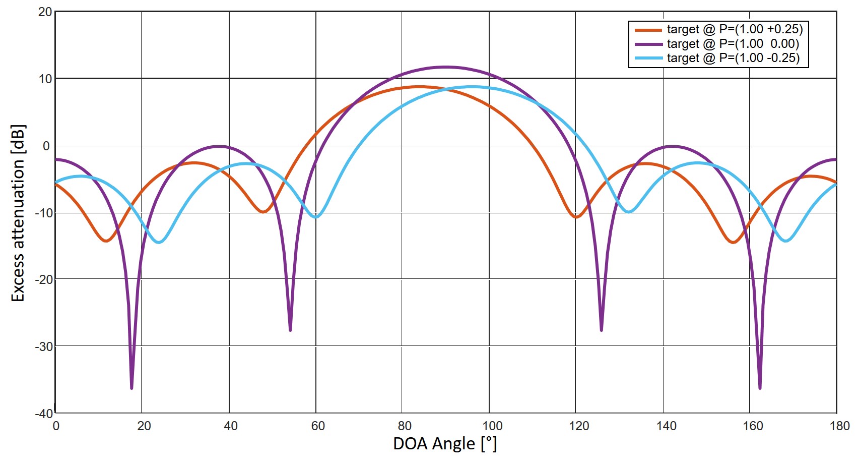
Figure 5: From top to bottom: a) target placement used for this test; b) excess attenuation expressed in terms of the DoA $\gamma$ of the array when the target $S$ is placed along the segment having distance $x=1$ m from the TX. Three different positions of the target $S$ are simulated at $(x,y)$: $(1.0,-0.25)$, $(1.0,0.0)$, and $(1.0,0.25)$; c) excess attenuation as observed on each single antenna without any array processing and for corresponding positions of the targets as above.

IV Preliminary results

In this section, we provide some preliminary results concerning the use of the array model of Sect. II vs the single-antenna model [7].

The carrier frequency $f_{c}$ is set to $f_{c}=2.4868$ GHz, and we used an UL array of $5$ omni-directional antennas ($M=2$) spaced at $d_{a}=\lambda/2$ as shown in the layout sketch described in Fig. 4. The length of the central link of the array (i.e., for $m=0$) is equal to $d=d_{0}=4$ m while all links of the array are horizontally placed at height $h=0.9$ m from the ground.

As far as the body model is concerned, the absorbing 2-D sheet that represents the target has size $a_{z}=0.9$ m and $a_{y}=0.275$ m (i.e. a total size of 1.80 m x 0.55 m). The target stands vertically on the floor, that is used only to support the target and does not have any EM influence on the radio links. The LoS of the central link will be the reference LoS line for the target positions with the origin of the axes placed in the TX as shown in Fig. 4.

Figs. 5,  6, and  7 show the behavior of the entire array, namely the array response, in terms of the excess attenuation $20\,\log_{10}|E_{R}^{(0)}/E^{(m)}|$ as a function of the DoA $\gamma$ and for different values of the $y$ displacement of the target $S$ (w.r.t. the central LoS). The locations of the target are limited to belong to the line at $\xi_{1}=x=1$ m that is orthogonal to the central LoS. Processing of the array signals to extract the response for varying DoA $\gamma$ is based on Fast Fourier Transform (FFT) and employs $N_{FFT}=257$ points.

For positions of the target $S$ near the LoS as in Figs. 5.a and 6.a, the extra attenuation for off-LoS positions (blue and yellow lines) are comparable with the one (red line) representing the target on the LoS (i.e., $\sim 15$ dB for $y=0$ m compared with $\sim 7$ dB for $y=\pm 0.25$ m). In addition, in Fig. 5.b the three positions, spaced by $0.25$ m, are clearly separable since they result in different array responses. Considering the closed-spaced positions (i.e., $5$ cm) of Fig. 6.b, the resulting extra attenuation values ($\sim 17$ dB) are now much closer to the one of target placed on the LoS, thus making more difficult to visually separate these locations. On the other hand, the targets are still distinguishable as they are associated with separable DoAs.

Figure 6: From top to bottom: a) target placement used for this test; b) excess attenuation of the array expressed in terms of the DoA $\gamma$ when the target $S$ is placed along the segment having distance $x=1$ m from the TX. Three very close positions of the target $S$ are simulated at $(x,y)$: $(1.0,-0.05)$, $(1.0,0.0)$, and $(1.0,0.05)$.

Figure 7: From top to bottom: a) target placement used for this test; b) excess attenuation of the array expressed in terms of the DoA $\gamma$ when the target $S$ is placed along the segment having distance $x=1$ m from the TX. Three widely spaced positions of the target $S$ are simulated at $(x,y)$: $(1.0,-1.0)$, $(1.0,0.0)$, and $(1.0,1.0)$.

To compare the excess attenuation results for the antenna array of Fig. 5.b vs the ones of the single antennas, Fig. 5.c show the excess attenuation for each antenna. Comparing for instance the results for the target on the LoS (red line), it is apparent that, Fig. 5.c, the attenuation ranges from $\sim 14$ dB to $\sim 16$ dB depending on the selected antenna, while in Fig. 5.b the maximum value of the excess attenuation is the averaged value of $\sim 15$ dB.

For positions of the target $S$ outside the link area (i.e., outside the first Fresnel’s ellipsoid, whose minor axis is $\sim 0.7$ m for the considered $f_{c}$), the influence due to the target is negligible. Some minor effects are visible in the nulls among the main and the side lobes, but they may be too weak to be exploited to identify the presence of the target in a real-world scenario, where there is always a certain degree of multipath.

We have also performed some preliminary evaluations of conventional [23] and MVDR (Minimum Variance Distortionless Response) [24] beamforming algorithms. However, for space constraints, the results will not be discussed in this paper. Although preliminary, the results are promising and highlight the possibility of using EM body models to develop ad-hoc array processing tools adapted for passive DFL applications.

V Conclusions

In this paper, we presented a tool for the simulation of the Electro-Magnetic (EM) effects of different body (i.e., target) positions inside a link area covered by an array of closely spaced omni-directional antennas. In the proposed preliminary study, we assessed the effects of the body on the antenna array response. In particular, we showed that for different target positions in the monitored area, the array is able to separate the contribution of the target when it is inside the first Fresnel’s ellipsoid. The effects of the target can be represented both in terms of excess attenuation, which depends on body relative position, and as alterations of the array response pattern which loosely depends on target Direction of Arrival (DoA), relative to the Line-of-Sight (LoS) path. The proposed method paves the way for future applications of multiple antenna processing techniques in device-free localization applications.

References

- [1] S. Savazzi, et al., ”Device-free Radio Vision for assisted living: leveraging wireless channel quality information for human sensing,” IEEE Signal Processing Magazine, vol. 33, no. 2, pp. 45–58, Mar. 2016.
- [2] G. Koutitas, ”Multiple human effects in body area networks,” IEEE Antennas and Wireless Propagation Letters, vol. 9, pp. 938–941, 2010.
- [3] R.C. Shit, et al., ”Ubiquitous Localization (UbiLoc): A Survey and Taxonomy on Device Free Localization for Smart World,” IEEE Communications Surveys & Tutorials, vol. 21, no. 4, pp. 3532–3564, Fourthquarter 2019.
- [4] J. Wilson, et al., ”Radio tomographic imaging with wireless networks,” IEEE Trans. on Mobile Comp., vol. 9, no. 5, pp. 621–632, May 2010.
- [5] A. Eleryan, et al., ”Synthetic generation of radio maps for device-free passive localization,” Proc. of the IEEE Global Telecommunications Conference GLOBECOM’11), pp. 1–5, 2011.
- [6] M. Mohamed, et al., ”Physical-statistical channel model for off-body area network,” IEEE Antennas and Wireless Propagation Letters, vol. 16, pp. 1516–1519, 2017.
- [7] V. Rampa, et al., ”EM models for passive body occupancy inference,” IEEE Antennas and Wireless Propagation Letters, vol. 17, no. 16, pp. 2517–2520, 2017.
- [8] V. Rampa, et al., Electromagnetic Models for Passive Detection and Localization of Multiple Bodies”, IEEE Transactions on Antennas and Propagation, vol. 70, no. 2, pp. 1462–1745, 2022.
- [9] V. Rampa, et al., ”EM Model-Based Device-Free Localization of Multiple-Bodies”, Sensors, vol. 21, art. 1728, 2021.
- [10] J. Wang, et al., ”Device-free localisation with wireless networks based on compressive sensing,” IET Communications, vol. 6, no. 5, pp. 2395–2403, Oct. 2012.
- [11] A.S.A. Sukor, et al., ”RSSI-Based for Device-Free Localization Using Deep Learning Technique,” Smart Cities, vol. 3, no. 2, pp. 444–455, 2020.
- [12] D. Halperin, et al., ”Predictable 802.11 packet delivery from wireless channel measurements,” ACM SIGCOMM Computer Communication Review, vol. 41, no. 4, p. 159–170, 2011.
- [13] Y. Xie, et al., ”Precise power delay profiling with commodity Wi-Fi,” IEEE Transactions on Mobile Computing, vol. 18, no. 6, pp. 1342–1355, 2018.
- [14] M. Atif, et al., ”Wi-ESP—A tool for CSI-based Device-Free Wi-Fi Sensing (DFWS),” Journal of Computational Design and Engineering, vol. 7, no. 5, pp. 644–656, Oct. 2020.
- [15] L. Zhang, et al., ”DeFi: Robust Training-Free Device-Free Wireless Localization With WiFi,” IEEE Transactions on Vehicular Technology, vol. 67, no. 9, pp. 8822–8831, Sept. 2018.
- [16] S. Shukri, et al., Enhancing the radio link quality of device-free localization system using directional antennas,” Proc. of the 7th International Conference on Communications and Broadband Networking, pp. 1–5, Apr. 2019.
- [17] D. Garcia, et al., ”POLAR: Passive object localization with IEEE 802.11 ad using phased antenna arrays,” Proc. of the IEEE INFOCOM 2020-IEEE Conference on Computer Communications, pp. 1838–1847, Jul. 2020.
- [18] W. Ruan, et al., ”Device-free indoor localization and tracking through Human-Object Interactions,” Proc. of the IEEE 17th International Symposium on A World of Wireless, Mobile and Multimedia Networks (WoWMoM’16), Coimbra, pp. 1–9, Jun. 2016.
- [19] V. Ojeda, et al., ”Rx position effect on Device Free Indoor Localization in the 28 GHz band,” Proc. of the IEEE Sensors Applications Symposium (SAS’2022), Sundsvall, pp. 1–6, Aug. 2022.
- [20] V. Rampa et al., ”Electromagnetic Models for Device-Free Radio Localization with Antenna Arrays,” Proc. of the IEEE-APS Topical Conf. on Antennas and Propagation in Wireless Communications, pp. 1–6, Sept. 2022.
- [21] F. Fieramosca, et al., ”Modelling of the Floor Effects in Device-Free Radio Localization Applications”, Proc. of the 17th European Conference on Antennas and Propagation (EuCAP’23), pp. 1–5, Florence, Mar. 2023.
- [22] A. Z. Elsherbeni, et al., ”Antenna Analysis and Design using FEKO Electromagnetic Simulation Software,” The ACES Series on Computational Electromagnetics and Engineering (CEME), SciTech Publishing, 2014.
- [23] J. Benesty, J., et al., ”A Brief Overview of Conventional Beamforming,” in Array Beamforming with Linear Difference Equations, Springer Topics in Signal Processing, vol 20, pp.13–21, 2021.
- [24] P. Stoica, et al., ”Robust Capon beamforming,” IEEE Signal Processing Letters, vol. 10, no. 6, pp. 172–175, June 2003.