Spectral complexity of deep neural networks

Abstract

It is well-known that randomly initialized, push-forward, fully-connected neural networks weakly converge to isotropic Gaussian processes, in the limit where the width of all layers goes to infinity. In this paper, we propose to use the angular power spectrum of the limiting fields to characterize the complexity of the network architecture. In particular, we define sequences of random variables associated with the angular power spectrum, and provide a full characterization of the network complexity in terms of the asymptotic distribution of these sequences as the depth diverges. On this basis, we classify neural networks as low-disorder, sparse, or high-disorder; we show how this classification highlights a number of distinct features for standard activation functions, and in particular, sparsity properties of ReLU networks. Our theoretical results are also validated by numerical simulations.

Keywords: Deep learning, neural networks, isotropic random fields, Gaussian processes, compositional kernels, angular power spectrum, model complexity

AMS subject classification (2010 MSC): 68T07, 60G60, 33C55, 62M15

1 Introduction

Allowing depth in neural networks has been instrumental in elevating them to the forefront of machine learning, paving the way for unprecedented results spanning from image recognition to natural language processing, up to the latest wonders of generative AI. Mirroring human abstraction, deep artificial networks extract relevant features in a hierarchical fashion, constructing more complex representations from simpler ones, and discerning high-dimensional patterns in reduced dimensions. On the other hand, just stacking more layers comes with its own risks, including overfitting, vanishing gradients, and general optimization instability, which makes depth a resource to use with care. Identifying measures of complexity capturing benefits and drawbacks of depth can thus provide a principled way to explain empirical behaviors and guide algorithmical choices.

Besides intuitions and practical evidence, a theoretical understanding of the role of depth in neural architectures remains a challenging endeavor. From an approximation perspective, the problem has been addressed in terms of depth separation. This approach goes beyond classical universal theorems (Cybenko, 1989; Hornik, 1991; Leshno et al., 1993; Pinkus, 1999), quantifying how the approximation error can scale exponentially along the width and polynomially along the depth (Telgarsky, 2016; Eldan and Shamir, 2016; Daniely, 2017; Safran and Shamir, 2017; Venturi et al., 2022). Recent work has extended these results to the infinite-width limit, shifting the representation cost from the number of units to a minimal weight norm (Parkinson et al., 2024). Other approaches have explored depth’s impact by estimating functional properties such as slope changes and number of linear regions in ReLU networks (Montufar et al., 2014; Hanin and Rolnick, 2019b; Goujon et al., 2024). Such quantities can be convexified by specific families of seminorms, thereby enforcing practical regularization strategies (Aziznejad et al., 2023). More generally, people have studied how the topology of the network changes with respect to its architecture, tracking the dependence of topological invariants on depth and activation function (Bianchini and Scarselli, 2014; Sun et al., 2016). Within this framework, Betti numbers have been notably considered and used to define suitable notions of complexity. More traditional model complexities such as VC-dimension and Rademacher have also been bounded for neural networks (Bartlett et al., 1998, 2019, 2017). However, such bounds can be too loose in typically overparameterized regimes.

An alternative point of view that is particularly relevant for our study is provided by the theories of reproducing kernels (Aronszajn, 1950) and Gaussian processes (Rasmussen and Williams, 2005). The link with neural networks may be sketched as follows. In suitable infinite-width limits, sometimes called kernel regimes, neural networks are equivalent to Gaussian processes, and are therefore characterized by positive definite kernels (Neal, 1996; Williams, 1996; Daniely et al., 2016; Lee et al., 2018; de G. Matthews et al., 2018; Hanin, 2023; Cammarota et al., 2023; Favaro et al., 2023; Jacot et al., 2018). Furthermore, the kernel corresponding to a deep neural network has an interesting compositional structure, namely it can be obtained by iteration of a fixed (shallow) kernel as many times as the number of hidden layers. This observation has sparked the idea of giving depth to kernel methods, with the hope of enhancing, if not feature learning, at least the expressivity of the model (Cho and Saul, 2009; Wilson et al., 2016; Bohn et al., 2019; Huang et al., 2023). In this context, potential benefits may be proved by checking whether the associated reproducing kernel Hilbert space (RKHS) actually expands when iterating the kernel. In a somewhat opposite yet related spirit, one can use the infinite-width limits to study RKHS as approximations of neural network models. It turns out that, even when the kernel is deep, the corresponding RKHS can be shallow, that is, it can be constant with respect to the depth of the kernel. More precisely, Bietti and Bach (2021) have shown that the spectrum of the integral operator associated to a deep ReLU kernel has the same asymptotic order regardless of the number of layers. As a consequence, ReLU RKHS of any depth are all equivalent, and therefore their structure fails in capturing the additional complexity induced by the depth.

In this paper we argue that the failure of the RKHS structure does not imply the general unsuitability of kernel regimes for studying depth in neural architectures. While Bietti and Bach (2021) look at the tail of the spectrum, which indeed completely determines the RKHS, we look at the whole spectrum, which may well depend on the depth even when the tail does not. Normalizing the variance of the neural network, we identify the angular power spectrum with a probability distribution on the non-negative integers, that we call the spectral law of the neural network. We denote by $X_{L}$ the associated random variable, stressing its dependence on the depth $L$. Our first main result (Theorem 1) characterizes neural networks based on the behavior of the moments of $X_{L}$. Depending on the form of the activation function, we identify three regimes: a low-disorder case (including the Gaussian and the logistic activations), where the finite moments of $X_{L}$ decay exponentially to zero as $L\to\infty$; a sparse case (including ReLU and Leaky ReLU), where the first two moments are uniformly bounded and the others grow polynomially – when they exist; and a high-disorder case (including the hyperbolic tangent), where the finite moments diverge exponentially. Our second main result (Theorem 2) studies the asymptotics of the spectral sequences $(X_{L})_{L\geq 1}$: in the low-disorder case, $X_{L}$ converges to zero as $L\to\infty$, implying that the random field concentrates on constant values; in the sparse case, $X_{L}$ is bounded with high probability uniformly in $L$, but diverges in any $\ell^{p}$ norm with $p>2$, which can be interpreted as a random field living on low frequencies but with some isolated spikes; in the high-disorder case, $X_{L}$ diverges exponentially, so that the field becomes more and more chaotic as $L$ grows.

Our results provide insights on the role of the activation function; in particular, the fact that the spectral sequences associated to ReLU networks are bounded in probability but diverge in almost all norms seems to agree with the intuition that such activation induces sparsity/self-regularization (Glorot et al., 2011). Based on these ideas, we introduce two indexes of complexity: the spectral effective support, which tells which multipoles capture most of the norm/variance of the network; and the spectral effective dimension, which measures the total dimension of the corresponding eigenspaces. Consistently with the previous considerations, these quantities are surprisingly low for ReLU networks: we show numerically that 99% or more of the norm is supported on less than a handful of spectral multipoles for arbitrarily large depth.

In conclusion, our key contributions may be summarized as follows.

1. We propose a new framework for studying the role of depth in neural architectures. Our approach is based on the theory of random fields, and more specifically on the spectral decomposition of isotropic random fields on the hypersphere.

2. Following this approach, we classify networks in three regimes where depth plays a significantly different role. In short, these regimes correspond to degenerate asymptotics (convergence to a trivial limit), asymptotic boundedness, and exponential divergence.

3. In particular, we show that ReLU networks fall into the intermediate regime, characterized by convergence in measure and divergence in $\ell^{p}$ norms for all $p>2$. This suggests that ReLU networks have a sparse/self-regularizing property, which may allow them to go deeper with less risk of overfitting.

4. Based on the above, we introduce a new simple notion of complexity for neural architectures, aimed at describing the effects of depth with respect to different choices of activation function.

The rest of the paper is organized as follows. In Section 2 we provide some background and notation; in Section 3 we state our main results and introduce our complexity measures. In Section 4 we validate our results and definitions by extensive numerical experiments. All proofs are collected in Appendix A.

2 Background and notation

2.1 Isotropic random fields on the sphere

Let $T:\,\mathbb{S}^{d}\times\Omega\to\mathbb{R}$ be a measurable application for some probability space $(\Omega,\mathcal{F},\mathbb{P})$. If $T$ is isotropic, meaning that the law of $T(\cdot)$ is the same as $T(g\cdot)$ for all $g\in SO(d)$ (the special group of rotation in $\mathbb{R}^{d+1}$), and it has finite covariance, then the spectral representation

$$T(x)=\sum_{\ell=0}^{\infty}\sum_{m=0}^{n_{\ell,d}}a_{\ell m}(\omega)Y_{\ell m}(x),\qquad x,y\in\mathbb{S}^{d}$$

holds in $L^{2}(\Omega\times\mathbb{S}^{d})$, i.e.

$$\lim_{M\to\infty}\mathbb{E}\left[\int_{\mathbb{S}^{d}}\left|T(x,\omega)-\sum_{\ell=0}^{M}a_{\ell,m}(\omega)Y_{\ell,m}(x)\right|^{2}\mathrm{d}x\right]=0\ .$$

Here we adopt a standard notation, and in particular we write $\{Y_{\ell m}\}$ for a $L^{2}$-orthonormal basis of real-valued spherical harmonics, which satisfy

$$\Delta_{\mathbb{S}^{d}}Y_{\ell,m}=-\ell(\ell+d-1)Y_{\ell m}\ ,\ \ell=1,2,\dots$$

where $\Delta_{\mathbb{S}^{d}}$ is the Laplace-Beltrami operator on the sphere. For all $\ell\in\mathbb{N}$, the dimension of the eigenspaces, i.e. the cardinality of the basis elements $\{Y_{\ell,m}\}$, is given by

$$n_{\ell,d}=\frac{2\ell+d-1}{\ell}\binom{\ell+d-2}{\ell-1}\sim\ell^{d-1}\ ,\ \text{as}\ \ell\rightarrow\infty\ .$$ (1)

Moreover, the random coefficients $\{a_{\ell,m}\}$ are such that

$$\mathbb{E}[a_{\ell,m}a_{\ell^{\prime},m^{\prime}}]=C_{\ell}\delta_{\ell}^{\ell^{\prime}}\delta_{m}^{m^{\prime}},\qquad\ell\in\mathbb{N},\,m=0,\dots,n_{\ell,d}$$

where $\{C_{\ell}\}_{\ell=0,1,2,\dots}$ is the angular power spectrum of $T$. Without loss of generality, we take the expected value of the field $T$ to be zero; for all $x,y\in\mathbb{S}^{d}$, the covariance is given by

$$\mathbb{E}[T(x)T(y)]=\sum_{\ell=0}^{\infty}C_{\ell}\frac{n_{\ell,d}}{\omega_{d}}G_{\ell;d}(\langle x,y\rangle)$$ (2)

where $\omega_{d}$ is the surface area of $\mathbb{S}^{d}$, and $G_{\ell;d}$ are the normalized Gegenbauer polynomials (see e.g. Marinucci and Rossi (2015) and A.1).

2.2 Random neural networks

Let us now recall briefly what we mean by a random neural network. For any given positive integers $L,d,n_{1}\dots,n_{L+1}\geq 1$ and $\sigma:\,\mathbb{R}\to\mathbb{R}$ such that $\Gamma_{\sigma}:=\mathbb{E}[\sigma(Z)^{2}]<\infty$ for $Z\sim\mathcal{N}(0,1)$, we denote by $T_{s}(\cdot)$ the sequence of random fields given by

$$T_{s}(x)=\begin{cases}W^{(0)}x+b^{(1)},&s=0\\ W^{(s)}\sigma(T_{s-1}(x))+b^{(s+1)},&s=1,\dots,L\end{cases},\qquad x\in\mathbb{S}^{d}$$ (3)

where $b^{(s)}\in\mathbb{R}^{n_{s}}$ and $W^{(s)}\in\mathbb{R}^{n_{s+1}\times n_{s}}$ are random vectors or matrices with independent components such that $b^{(s)}_{i}\sim N(0,\Gamma_{b})$, $W_{ij}^{(0)}\sim\mathcal{N}(0,\Gamma_{W_{0}})$ and $W_{ij}^{(\ell)}\sim\mathcal{N}\left(0,\frac{\Gamma_{W}}{n_{\ell}}\right)$ for some positive constants $\Gamma_{b},\Gamma_{W_{0}},\Gamma_{W}$. To simplify the notation, in the sequel we shall take $n_{0}=d+1$.

It is well established (see (Neal, 1996; Hanin, 2023; Favaro et al., 2023; Cammarota et al., 2023) and the references therein) that for all $s>1$, as $n_{1},\dots,n_{s}\to\infty$, the random field $T_{s}$ converges weakly to a Gaussian vector field with $n_{s+1}$ i.i.d. centered components $(T_{i;s}^{\star})_{i=1,\dots,n_{s+1}}$. We denote the corresponding limiting covariance kernel by $K_{s}$. More precisely, assuming the standard calibration condition $\Gamma_{b}+\Gamma_{W_{0}}=1$ and taking $\Gamma_{W}=(1-\Gamma_{b})\Gamma_{\sigma}^{-1}$ (so that each layer has unit variance), we have that $K_{1}(x,y)=\kappa_{1}(\langle x,y\rangle)$ only depends on the angle between $x$ and $y$, while $K_{s}(x,y)=\kappa_{s}(\langle x,y\rangle)$ with

$$\kappa_{s}(u)=\kappa_{1}\circ\dots\circ\kappa_{1}(u)$$

composed $s-1$ times. Furthermore $\kappa_{1}(1)=\kappa_{s}(1)=1$ (see Lemma 38 below for more details).

3 Main results

Let $T_{L}$ be a sequence of isotropic random fields on the sphere. By the Schoenberg theorem, the covariance kernel of $T_{L}$ can be expressed as

$$K_{L}(x,y)=\kappa_{L}(\langle x,y\rangle)=\sum_{\ell=0}^{\infty}D_{\ell;\kappa_{L}}G_{\ell;d}(\langle x,y\rangle)$$

where $G_{\ell;d}$ are the normalized Gegenbauer polynomials. Since $G_{\ell;d}(1)=1$, we can then associate with each $T_{L}$ an integer-value random variable $X_{L}$ with the following probability mass function:

$$\mathbb{P}(X_{L}=\ell)=D_{\ell;\kappa_{L}}\ ,\ \ell=1,2,\dots\ .$$ (4)

When $T_{L}$ is a random field associated to a neural network with depth $L$, we call the previous density the neural network spectral law. The main idea of our paper is that the asymptotic behavior of this probability distribution when $L$ increases provides insights on important features of the corresponding neural architecture. In particular, our first main result characterizes neural networks by studying the moments of their spectral law.

Theorem 1

Let $T_{L}:\,\mathbb{S}^{d}\to\mathbb{R}$ denote one of the components of the limiting Gaussian process $(T_{i;L}^{\star})_{i=1,\dots,n_{L+1}}$ and let $\{X_{L}\}_{L=1,2,\dots}$ be the associated sequence of random variables. We assume that the function $\kappa:[-1,1]\to\mathbb{R}$, defined by $\mathbb{E}[T_{1}(x)T_{1}(y)]=\kappa(\langle x,y\rangle)$, admits the first derivative at $1$.

• (Low-disorder case) If $\kappa^{\prime}(1)<1$, then:

  • If $\kappa$ is infinitely differentiable in a neighborhood of $1$, then $X_{T_{L}}$ has all finite moments. These moments decay exponentially to zero as $L$ diverges, and in particular for the even moments we have

    $$\mathbb{E}[X_{L}^{2n}]=\kappa^{\prime}(1)^{nL}\left(C_{n}+o(1)\right)\quad as\ L\rightarrow\infty$$ (5)

    where $C_{n}$ is a constant depending only on $d$ and the first $n$ derivatives of $\kappa$ at the origin.

  • If $\kappa$ is differentiable only $r$ times in a neighborhood of $1$, then $X_{L}$ has $2r$ finite moments that decay as in (5). On the other hand, for all $n>r$ and $M>0$ there exist constants $\xi_{M}\in(0,1)$ (not depending on $L$ and $n$) and $C_{n;M}>0$ (not depending on $L$) such that

    $$\mathbb{E}[X_{L}^{2n}\mathbb{I}_{[0,M]}(X_{L})]=\xi_{M}^{nL}\left(C_{n;M}+o(1)\right)\ as\ L\rightarrow\infty\ .$$ (6)

• (Sparse case) If $\kappa^{\prime}(1)=1$, then

  $$0\leq\mathbb{E}[X_{L}]\leq 1\ ,\qquad 1\leq\mathbb{E}[X_{L}^{2}]\leq d\ .$$ (7)

  Furthermore:

  • If $\kappa$ is infinitely differentiable in a neighborhood of $1$, then $X_{T_{L}}$ has all finite moments. The moments greater than the second grow polynomially in $L$:

    $$\mathbb{E}[X_{L}^{2n}]=L^{n-1}(F_{n}+o(1))\quad\text{ as }L\to\infty$$ (8)

    where $F_{n}$ is a constant depending only on $d$, $n$ and $\kappa^{\prime\prime}(1)$.

  • If $\kappa$ is only $r$ times differentiable in a neighborhood of $1$, then $X_{T_{L}}$ has $2r$ finite moments that grow as in (8). Therefore, there exists a divergent nondecreasing sequence $(M_{i})$ such that, for all $i$,

    $$\xi_{i}^{L}\left(G_{n,i}+o(1)\right)\leq\frac{\mathbb{E}\left[X_{L}^{n}\mathbb{I}_{[M_{i},M_{i+1}]}(X_{L})\right]}{\mathbb{E}\left[X_{L}^{n}\mathbb{I}_{[0,M_{i}]}\right]}\leq\xi_{i}^{L}\left(H_{n,i}+o(1)\right)\quad\text{ as }L\to\infty\ ,$$ (9)

    where $\xi_{i}>1$ depends only on $\kappa$, $M_{i}$ and $M_{i+1}$ and $G_{n,i},H_{n,i}$ do not depend on $L$.

• (High-disorder case) If $\kappa^{\prime}(1)>1$, then:

  • If $\kappa$ is infinitely differentiable in a neighborhood of $1$, then $X_{L}$ has all finite moments. These moments grow exponentially in $L$ as in (5).

  • If $\kappa$ is only $r$ times differentiable in a neighborhood of $1$, then $X_{L}$ has $2r$ finite moments that grow as in (5). On the other hand, for sufficiently large $M>0$, the truncated moments satisfy (6) with $\xi_{M}>1$.

Our second main result refines Theorem 1 by characterizing directly the asymptotics of the spectral sequences associated to the field.

Theorem 2

Under the same notation and conditions as in Theorem 1, we have the following.

• (Low-disorder case) If $\kappa^{\prime}(1)<1$, then

  $$X_{L}\xrightarrow{P}0\ .$$

• (Sparse case) If $\kappa^{\prime}(1)=1$, then for all $\varepsilon>0$ there exists $n_{\varepsilon}$ such that

  $$\mathbb{P}(X_{L}\leq n_{\varepsilon})\geq 1-\varepsilon\qquad\text{for all }L.$$

• (High-disorder case) If $\kappa^{\prime}(1)>1$, then there exists a constant $c>1$ such that the random sequence $X_{L}/c^{L}$ is bounded and bounded away from zero in probability.

To substantiate our results, in Table 1 we classify commonly adopted activation functions into one of the three categories introduced in Theorem 1; see Di Lillo for the explicit computations of $\kappa^{\prime}(1)$ for the various activation functions.

Activation	$\sigma(x)$	Category
Logistic	$\frac{1}{1+e^{-x}}$	L
GELU	$x\Phi(x)$	L
ReLU	$x\mathbb{I}_{[0,+\infty)}(x)$	S
LReLU	$x\mathbb{I}_{[0,+\infty)}(x)+0.001x\mathbb{I}_{(-\infty,0)}(x)$	S
PReLU	$x\mathbb{I}_{[0,+\infty)}(x)+ax\mathbb{I}_{(-\infty,0)}(x)$	S
RePU$(p\geq 2)$	$x^{p}\mathbb{I}_{[0,+\infty)}(x)$	H
Hyperbolic tangent	$\tanh(x)$	H
Normal cdf	$\Phi(x)$	H
Exponential	$e^{ax}$	L $|a|<1$, S $|a|=1$, H $|a|>1$
Gaussian	$e^{-ax^{2}/2}$	L $a^{2}<\overline{a}$, S $a^{2}=\overline{a}$, H $a^{2}>\overline{a}$
Cosine	$\cos(ax)$	L $|a|<1.09$, H $|a|>1.09$

Table 1: Classification into the three categories of Theorem 1 (L = Low-disorder , S = Sparse and H = High-disorder) for standard activation functions. For the logistic activation function, $\kappa^{\prime}(1)$ was calculated numerically. For the Gaussian, $\overline{a}=1+\sqrt{2}$.

Remark 3

In the Low-disorder case $\kappa^{\prime}(1)<1$, the fact that $X_{L}$ goes to zero implies that, for large $L$, the associated sequence of random fields $T_{L}$ is close to a sequence of constant fields, where the value of the constants can vary from $L$ to $L$, but not over the points of the sphere for a given $L$.

Remark 4

The bounds in Theorem 1 are expressed only for even moments, but it is immediate to derive inequalities for the odd moments as well since the random variables $X_{L}$ are non-negative.

For isotropic kernels, it is well-known that the corresponding Reproducing Kernel Hilbert Spaces are equivalent to Sobolev spaces, with associated norm penalized by the angular power spectrum (Lang and Schwab, 2015). This justifies viewing general RKHS as generalized Sobolev spaces: in this interpretation, our results suggest that, while Sobolev norms are blind to depth (Bietti and Bach, 2021), the full angular power spectrum itself captures important information, and can thus be used to define a proper notion of depth-dependent complexity. This is the goal of the next definition.

Definition 5

(Spectral effective support and spectral effective dimension) Let $T_{L}:\,\mathbb{R}^{d}\to\mathbb{R}$ be a random neural network defined as in (3), and let $X_{L}$ be the associated random variable as in (4). The spectral $\alpha$-effective support ($\alpha\in(0,1)$) of $T_{L}$ is

$$\mathcal{C}_{\alpha}=\min\Bigg{\{}n\in\mathbb{N}\;\Bigg{|}\;\sum_{\ell=0}^{n}\mathbb{P}(X_{L}=\ell)\geq 1-\alpha\Bigg{\}}\,.$$

The spectral $\alpha$-effective dimension of $T_{L}$ is

$$\mathcal{D}_{\alpha}=\sum_{\ell=0}^{C_{\alpha}}n_{\ell;d}$$

where $n_{\ell;d}$ is defined in (1).

Remark 6

Heuristically, if a neural network with a given architecture has a spectral $\alpha$-effective support equal to $\mathcal{C}_{\alpha}$, then $\mathcal{C}_{\alpha}$ multipoles (equivalently, harmonic frequencies) are sufficient to explain $(1-\alpha)\%$ of its random norm (i.e. variance), and hence the corresponding random field is “close” (in the $L^{2}$ sense) to a polynomial with degree $\mathcal{C}_{\alpha}$. The dimension of the corresponding vector spaces depends also on the dimension of the domain $\mathbb{S}^{d}$, and it grows in general as $\mathcal{D}_{\alpha}\simeq\mathcal{C}_{\alpha}^{d-1}$. Some numerical evidence to support these claims is given below, see Tables 3 and 4 in Section 4.

Remark 7

In view of Definition 5 we can reinterpret the classification given in Theorems 1 and 2: in the low-disorder case, the complexity decays to $0$ exponentially fast in $L$; in the sparse case, the complexity is bounded from above uniformly over $L$; in the high-disorder case, the complexity diverges exponentially in $L$.

Remark 8

It is interesting to compute some explicit bounds for ReLU. In $d=2$, using the Markov inequality, it is immediate to see that more than $\-\mathbb{E}[X_{L}^{2}]/10^{2}=0.98$ of the probability mass is (uniformly in $L$) in the first $10$ multipoles, which span a vector space of dimension of order $100$. This is only an upper bound, and indeed the simulations in Table 3 (Section 4) below show that up to $99\%$ of the probability mass is confined in the first two multipoles as $L$ increases. This is rather surprising, keeping in mind that, for large $L$, the neural network could have millions, if not billions, of parameters.

Remark 9 (On the peculiar properties of ReLU)

A comprehensive inspection of the previous results and definitions highlights some peculiarities of the ReLU activation, which may perhaps explain some of its empirical success. On the one hand, the spectral effective dimension remains bounded at any depth $L$, as illustrated in the simulations of Section 4. This naturally suggests that ReLU networks may be less prone to overfitting phenomena. On the other hand, the divergence of ReLU moments of order larger than $2$ suggests that there exist sparse components at high frequencies, which seems to explain the approximation capabilities of ReLU networks at large depth. Our findings in this paper seem consistent with deterministic characterizations of the expressivity of ReLU networks given for instance by Hanin and Rolnick (2019b) and Hanin and Rolnick (2019a). See also (Daubechies et al., 2022) and the references therein.

Remark 10

It should be noted that, in the ReLU case (see Proposition 12 and Proposition 16),

$$(d-1)\mathbb{E}[X_{L}]+\mathbb{E}[X_{L}^{2}]=d\kappa^{\prime}(1)^{L}$$

implies that $X_{L}\overset{p}{\to}1$ for $d\rightarrow\infty$, . Indeed, we have

$$\lim_{d\rightarrow\infty}\mathbb{E}[X_{L}]=\frac{d}{d-1}-\frac{1}{d-1}\mathbb{E}[X_{L}^{2}]=1$$

and, on the other hand,

$$(\mathbb{E}[X_{L}])^{2}\leq\mathbb{E}[X_{L}^{2}]\leq d-(d-1)\mathbb{E}[X_{L}]\leq d-(d-1)(1+\epsilon)$$

whence the result follows. Heuristically, this implies that, as the dimension diverges, the random ReLU network converges in probability to a random linear functional (i.e. its spectral mass is concentrated on the first multipole $\ell=1$).

4 Numerical evidence

We now present numerical experiments to illustrate our results; the corresponding code is publicly available at https://github.com/simmaco99/SpectralComplexity and it is based on the HealPIX package for spherical data analysis (Gorski et al., 2005).

Our first goal is to visualize the different role played by the network depth in the three scenarios considered above in Theorems 2 and 1. In particular, Figure 1 shows random neural networks generated according to different activation functions in the three classes (low-disorder, sparse, high-disorder), for growing $L=1,20,40,60,80$. We focus on the following activation functions.

• (Low-disorder case) Here we take the Gaussian activation function

  $$\sigma_{1}(x)=e^{-x^{2}/2}\ ;$$

  by Lemma 39, the normalized covariance kernel is given by

  $$\kappa(u)=\sqrt{\frac{3}{4-u^{2}}}\ .$$

  A trivial calculation shows that $\kappa^{\prime}(1)<1.$

  The simulations reported in the first column of Figure 1 are indeed perfectly consistent with the previous results. In particular, starting from $L$ of order $20$ we obtain random fields which are very close to constant over the whole sphere; the analogous pictures for higher values of $L$ are not reported in  Figure 2, because their appearance is basically identical.

• (Sparse case) Here we focus on the celebrated and widely adopted ReLU activation function, that is

  $$\sigma_{2}(x)=\max(0,x)\ .$$

  It is known (see for instance (Cho and Saul, 2011)) that the normalized associated kernel is given by

  $$\kappa(u)=\frac{1}{\pi}\left(u(\pi-\arccos(u))+\sqrt{1-u^{2}}\right)\ .$$

  A simple calculation shows that $\kappa^{\prime}(1)=1$. The pictures fully confirm what is expected; in particular, the corresponding random field converges to Gaussian realizations with an angular power spectrum dominated by very few low multipoles, as made evident by the overwhelming presence of large scale fluctuations at every depth $L$.

• (High-disorder case) Let us finally consider the sigmoid activation function

  $$\sigma_{3}(x)=\tanh(x)\ .$$

  The associated kernel is not known analytically (to the best of our knowledge) but Lemma 40 shows that the derivative at the origin is greater than one. In view of the third part of Theorems 1 and 2, we know that the corresponding random fields have angular power spectra that diverge to infinity exponentially as the depth increases. Because of this, we expect more and more “wiggly” realizations at larger depths; this is indeed fully confirmed by the plots on the right column of Figures 1 and 2. The comparison between ReLU and sigmoid realizations are – we believe – extremely illuminating.

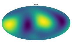
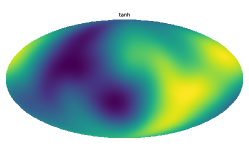
(a) $1$-hidden layer

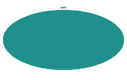
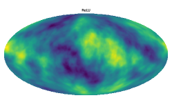
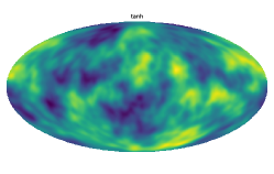
(b) $20$-hidden layer

Figure 1: Mollweide projection of a random neural network $T_{L}:S^{2}\to\mathbb{R}$ with varying depth $L=1,20$ (from top to bottom). The activation functions are $\sigma_{1}(x)=e^{-x^{2}/2}$, $\sigma_{2}(x)=\max(0,x)$ and $\sigma_{3}=\tanh(x)$ (from left to right). The fields were obtained through a Monte Carlo simulation (1000 replicas). The size of hidden layers is fixed at $1000$ neurons and the resolution of the map is $0.11$ deg. Important: note that the color bars are very different. Refer to Table 2, which displays the range of values assumed by the fields; in the plot, the values of the field are approximated to the 3rd decimal digit.

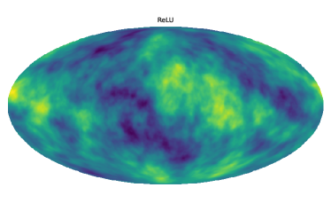
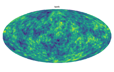
(a) $40$-hidden layer

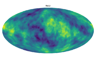
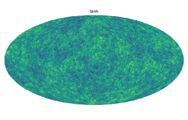
(b) $60$-hidden layer

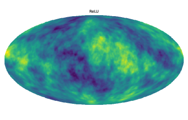
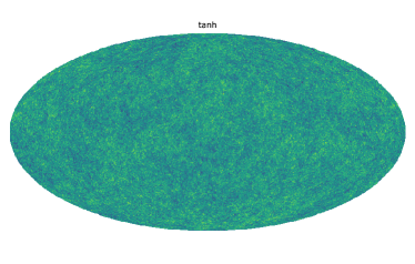
(c) $90$-hidden layer

Figure 2: Same as Figure 1: ReLU on the left, tanh on the right. The maps corresponding to Gaussian activations are dropped because they are simply constant on the sphere.

Depth	Gaussian		ReLU		$\tanh$
	min	max	min	max	min	max
$1$	$-0.5536$	$0.64094$	$-1.46433$	$1.53117$	$-1.73473$	$1.73473$
$20$	$0.00013$	$0.00016$	$-0.57855$	$0.69359$	$-2.92493$	$2.92493$
$40$	$0.07904$	$0.07904$	$-0.42578$	$0.46043$	$-3.9283$	$3.9283$
$60$	$-0.0072$	$-0.0072$	$-0.43158$	$0.29306$	$-4.65288$	$4.65288$
$80$	$0.00992$	$0.00993$	$-0.37657$	$0.26124$	$-4.88463$	$4.88463$

Table 2: The maximum and minimum values of the field with different activation functions; the results were obtained computing the means of $1000$ Monte Carlo iterations.

To quantify the fluctuations of the fields, we computed minima and maxima through $1000$ Monte Carlo realizations; the results are reported in Table 2.

We produce further evidence estimating by a Monte Carlo simulation the numerical values of the angular power spectra under different architectures; The results are given in Figure 3 for ReLU, and in Figures 4 and 5 for the sigmoid activation. We see for ReLU how the power spectrum concentrates on the very first multipoles as $L$ increases. On the contrary, in the sigmoid case the power spectrum shifts further and further to the right at larger depths.

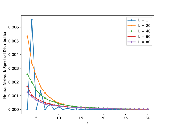
(a) $\ell$ from $3$ to $30$

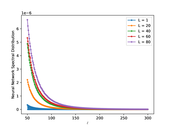
(b) $\ell$ from $50$ to $300$

Figure 3: Angular power spectrum for the ReLU activation function and different depths $L=1,20,40,60,80$. Figure (a) and (b) are a magnification of the same plot over different multipoles: $99\%$ of the mass is supported in the first 2 multipoles, and for clarity, only multipoles greater than $2$ are reported. The angular power spectrum is computed using $200$ Monte Carlo iterations; the size of hidden layers is fixed at $n=500$ and the resolution of the map is $0.11$ deg.

(a) $\ell$ from $2$ to $100$

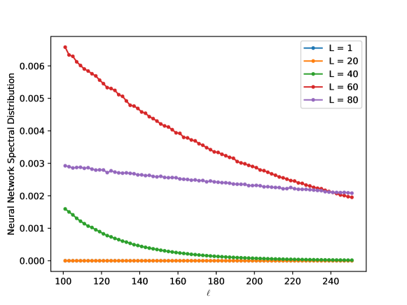
(b) $\ell$ da $100$ a $250$

Figure 4: Angular power spectrum for sigmoid activation functions at different depths $L=1,20,40,60,80$. Figure (a) and (b) are a magnification of the same plot over different multipoles; only odd multipoles are considered because even ones are equal to zero (see Lemma 40 for more details). The angular power spectrum is computed by means of $200$ Monte Carlo iterations; the size of hidden layers are fixed at $500$ neurons and the resolution of the map is $0.11$ deg.

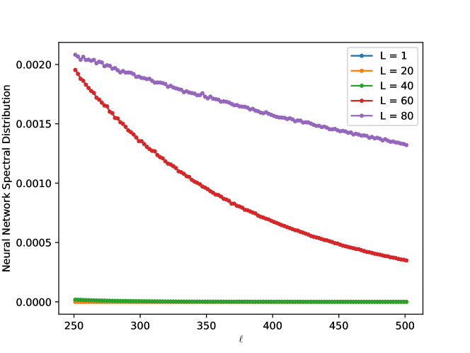
Figure 5: Magnification of the same plot as in Figure 4 over multipoles in the range $[250,500]$.

Finally, we provide some numerical evidence for our proposed notions of spectral effective support and dimension. In particular, Table 3 shows that for ReLU $99\%$ and more of the angular power spectrum concentrates on very few low multipoles, in the order of 1 or 2; correspondingly, in the $L^{2}$ sense the random neural network is very well approximated by a polynomial function belonging to a vector space of dimension 9 (for $L=60$) or even $4$ (for $L=80$) (when the input space is bidimensional). On the other hand, in the case of the sigmoid it takes several hundreds of multipoles to achieve a similar $L^{2}$ approximation in the order of $99\%$, see the two last columns of Table 4. Correspondingly, it takes a vector space of dimension $10^{6}$ or larger for a suitable approximation, showing that no sparsity is present here.

depth	$0.01$	$0.005$	$0.001$	$0.0005$	$0.0001$
$1$	$2$	$4$	$6$	$8$	$14$
$20$	$4$	$7$	$15$	$20$	$36$
$40$	$3$	$7$	$18$	$25$	$48$
$60$	$2$	$4$	$17$	$25$	$52$
$80$	$1$	$4$	$18$	$27$	$59$

(a)

depth	$0.01$	$0.005$	$0.001$	$0.0005$	$0.0001$
$1$	$9$	$25$	$49$	$81$	$225$
$20$	$25$	$64$	$256$	$441$	$1369$
$40$	$16$	$64$	$361$	$676$	$2401$
$60$	$9$	$25$	$324$	$676$	$2809$
$80$	$4$	$25$	$361$	$784$	$3600$

(b)

Table 3: (a) Spectral $\alpha$-effective support and (b) spectral $\alpha$-effective dimension for ReLu activation function for $\alpha=0.01,0.005,0.001,0.0005,0.0001$ and $L=1,20,40,60,80$. These values are computed by means of $200$ Monte Carlo simulations, the width of hidden layers is fixed at $500$ neurons and the resolution of the map is $0.11$ deg.

depth	$0.5$	$0.4$	$0.3$	$0.2$	$0.1$	$0.01$
$1$	$1$	$1$	$1$	$1$	$1$	$3$
$20$	$3$	$3$	$5$	$7$	$9$	$15$
$40$	$15$	$21$	$29$	$39$	$59$	$135$
$60$	$77$	$103$	$141$	$195$	$287$	$547$
$80$	$399$	$541$	$727$	$981$	$1339$	$>1537$

(a)

depth	$0.5$	$0.4$	$0.3$	$0.2$	$0.1$	$0.01$
$1$	$4$	$4$	$4$	$4$	$4$	$16$
$20$	$16$	$16$	$36$	$64$	$100$	$256$
$40$	$256$	$484$	$900$	$1600$	$3600$	$18496$
$60$	$6084$	$10816$	$20164$	$38416$	$82944$	$300304$
$80$	$16000$	$293764$	$529984$	$964324$	$1795600$	$>2,359\times 10^{6}$

(b)

Table 4: (a) Spectral $\alpha$-effective support and (b) spectral $\alpha$-effective dimension for the sigmoid activation function for $\alpha=0.5,0.4,0.3,0.2,0.1,0.01$ and $L=1,20,40,60,80$. These values are computed by means of $200$ Monte Carlo simulations, the width of hidden layers is fixed at $500$ neurons and the resolution of the map is $0.11$ deg.

5 Conclusions and future work

We believe that this paper opens several paths for further research; among these, we mention the following.

• The possibility of exploring the geometry of the random fields associated with a given architecture, for instance, characterizing the expected behavior of their critical points and the Lipschitz-Killing curvatures of their excursion sets (see (Adler and Taylor, 2007),  (Azais and Wschebor, 2009)). This topic is already the subject of ongoing research.

• The investigation of covariance kernels and the corresponding neural network regime when both width and depth are finite, but tend jointly to infinity. It is not difficult to show that the associated random fields are still isotropic (due to rotational invariance of Gaussian variables), but the behavior of their covariance kernels will be different and presumably depend on the ratio $L/n$, in analogy with what was observed for the asymptotic Gaussianity in (Hanin, 2023).

• The investigation of covariance kernels and geometry of excursion sets for more general network architectures, for instance not necessarily feed-forward or fully connected. The most promising alternative seems to be convolutional neural network, which have very similar associated covariance kernels.

• The characterization of the exact distribution for limiting random variables associated to different choices of activation functions.

• The analysis of the limiting behavior when the dimension $d$ grows; we have showed above that in the ReLU case there is asymptotic convergence to a linear process, and it seems important to investigate further some related issues, in particular the asymptotic behavior when $d$ and $L$ grow jointly.

These open problems are currently being explored by the authors.

Acknowledgments and Disclosure of Funding

This work was partially supported by the MUR Excellence Department Project MatMod@TOV awarded to the Department of Mathematics, University of Rome Tor Vergata, CUP E83C18000100006. We also acknowledge financial support from the MUR 2022 PRIN project GRAFIA, project code 202284Z9E4, the INdAM group GNAMPA and the PNRR CN1 High Performance Computing, Spoke 3.

Appendix A Proofs

In this Appendix we collect all the proofs of this paper. In particular, in Section A.1 we recall the definition of Gegenbauer polynomials along with some of their characteristics; in Section A.2 we derive analytic relationships between kernel functions and angular power spectra; in Section A.3 we study the asymptotic behavior of iterated kernels and their derivatives; in Section A.4 we investigate the asymptotic of spectral moments for the low- and high-disorder cases; in Section A.5 we consider the asymptotic of spectral moments for the intermediate (sparse) case; in Section A.6 we study the moments of truncated sequences, and finally in Section A.7 we give the proofs of our two main Theorems. In Section A.8 we compute the kernel associated to Gaussian activation functions and we bound the derivative of the normalized kernel associated to hyperbolic tangent activation functions.

A.1 Gegenbauer polynomials

For any given $\lambda>0$ and any integer $n\geq 0$, the ultraspherical polynomial of degree $n$, denoted by $P_{n}^{(\lambda)}$, is defined by the expansion

$$(1-2rt+r^{2})^{-\lambda}=\sum_{n=0}^{\infty}P_{n}^{(\lambda)}(t)r^{n},\qquad t\in[-1,1]$$

In particular, one can prove that (Szegő, 1975, p. 80):

$$P_{n}^{(\lambda)}(1)=\binom{n+2\lambda-1}{n}$$

and (Szegő, 1975, p. 81):

$$\frac{\mathrm{d}}{\mathrm{d}x}P_{n}^{(\lambda)}(x)=2\lambda P_{n-1}^{(\lambda+1)}(x)\ .$$

Moreover (Abramowitz and Stegun, 1965, p. 774),

$$\int_{-1}^{1}P_{n}^{(\lambda)}(t)P_{m}^{(\lambda)}(t)(1-t^{2})^{\lambda-1/2}\mathrm{d}t=\frac{2\pi\Gamma(n+2\lambda)}{n!(n+\lambda)2^{2\lambda}\Gamma(\lambda)^{2}}\delta_{n}^{m}\ .$$

Let $d>2$ be an integer; for all $n\in\mathbb{N}$ we define normalized Gegenbauer polynomials $G_{\ell,d}$ as

$$G_{\ell;d}(x):=P_{\ell}^{((d-1)/2)}(x)\binom{\ell+d-2}{\ell}^{-1}\ .$$ (10)

By the previous formulae, it can be checked immediately that

$$G_{\ell;d}(1)=1$$

and

$$\frac{\mathrm{d}}{\mathrm{d}x}G_{\ell,d}(x)=\frac{\ell(\ell+d-1)}{d}G_{\ell-1;d+2}(x)\ .$$ (11)

A.2 On the link between kernel derivatives and spectral moments

Let $\kappa:[-1,1]\to\mathbb{R}$ be a continuous covariance kernel corresponding to a unit-variance, isotropic random field on $\mathbb{S}^{d}$; by Schoenberg’s Theorem we have the identity

$$\kappa(t)=\sum_{\ell=0}^{\infty}D_{\ell,\kappa}G_{\ell;d}(1),\quad t\in[-1,1]$$ (12)

where $G_{\ell;d}$ are the Gegenbauer polynomials and $(D_{\ell,\kappa})_{\ell\in\mathbb{N}}$ is a sequence of non-negative numbers such that

$$\kappa(1)=\sum_{\ell=0}^{\infty}D_{\ell;\kappa}=1\ .$$

Our first definition associates with these weights summing to one a discrete probability function and the associated random variable.

Definition 11

We define $X_{\kappa}$ the random variable associated to the kernel $\kappa$ if its discrete probability function satisfies

$$\mathbb{P}(X_{\kappa}=\ell)=D_{\ell;\kappa}\ ,\ \ell=0,1,2,....$$

The Definition 11 is consistent with that of Neural Network Spectral Distribution (see (4)); in particular, Schoenberg’s Theorem guarantees that there is a unique variable associated to a given isotropic random field with covariance kernel $\kappa$.

Proposition 12

If the covariance kernel $\kappa$ is $n$ times differentiable in a neighborhood of $1$ then $X_{\kappa}$ has $2n$ finite moments. Furthermore, for all $s\leq n$ these moments satisfy the identity

$$\sum_{i=0}^{2s}a_{i}^{s}\mathbb{E}[X_{\kappa}^{s}]=\frac{(d+2s-2)!!}{(d-2)!!}\kappa^{(s)}(1)$$ (13)

where

$$a_{i}^{s+1}=a_{i-2}^{s}+(d-1)a_{i-1}^{s}-s(d+s-1)a_{i}^{s}\qquad s\geq 0,\ \ 1\leq i\leq 2s\ ,$$

$$a_{i}^{s}=0 s\geq 0,\ \ i\leq 0\text{ or }i>2s$$

with the initial condition

$$a_{i}^{1}=\begin{cases}d-1&\text{ if }i=1\\ 1&\text{ if }i=2\\ 0&\text{ otherwise}\end{cases}\ .$$ (14)

Proof Using the derivation formula for Gegenbauer polynomials (see eq. 11), and since the $s$-th derivative of $\kappa$ in a neighborhood of $1$ exists, we can differentiate equation (12) $s$ times and interchange the series with the derivative. Hence we obtain

$$\kappa^{(s)}(1)=\sum_{\ell=0}^{\infty}D_{\ell;\kappa}\left(\prod_{j=0}^{s-1}\frac{(\ell-j)(\ell+d+j-1)}{d+2j}\right)\ .$$

Denoting by $p_{s}$ the polynomial

$$p_{s}(x)=\prod_{j=0}^{s-1}(x-j)(x+d+j-1)$$ (15)

we have

$$\frac{(d+2s-2)!!}{(d-2)!!}\kappa^{(s)}(1)=\sum_{\ell=0}^{\infty}D_{\ell;\kappa}p_{s}(\ell)=\mathbb{E}\left[p_{s}(X_{\kappa})\right]\ .$$

It follows that $X_{\kappa}$ has $2s$ finite moments, as claimed.

Let us now proceed to establish eq. 13; it is easy to observe that $\deg p_{s}=2s$ and $p_{s}(0)=0$. Therefore, there exist $(a_{i}^{s})_{i=1,\dots,2s}$ such that $a_{0}^{s}=0$ and

$$p_{s}(x)=\sum_{i=1}^{2s}a_{i}^{s}x^{i}\ .$$

From equation (15) it follows that $p_{1}(x)=x^{2}+(d-1)x$ and hence (14) is valid. Our idea is to proceed by induction on all other values of $s$. More precisely, from (15) and some simple algebraic manipulations we obtain also

$$p_{s+1}(x)=(x-s)(x+d+s-1)p_{s}(x)$$

and in particular

$$p_{s+1}(x)= (x-s)(x+d+s-1)\sum_{i=1}^{2s}a_{i}^{s}x^{i}=\left(x^{2}+(d-1)x-s(d+s-1)\right)\sum_{i=1}^{2s}a_{i}^{s}x^{i}$$

$$= \sum_{i=1}^{2s}a_{i}^{s}x^{i+2}+(d-1)\sum_{i=1}^{2s}a_{i}^{s}x^{i+1}-s(d+s-1)\sum_{i=1}^{2s}a_{i}^{s}x^{i}$$

$$= \sum_{i=3}^{2(s+1)}a_{i-2}^{s}x^{i}+(d-1)\sum_{i=2}^{2s+1}a_{i-1}^{s}x^{i}-s(d+s-1)\sum_{i=1}^{2s}a_{i}^{s}x^{i}$$

$$= \sum_{i=1}^{2(s+1)}\left(a_{i-2}^{s}+(d-1)a_{i-1}^{s}-s(d+s-1)a_{i}^{s}\right)x^{i}$$

$$-(a_{-1}^{s}x+a_{0}^{s}x^{2})-(d-1)(a_{0}^{s}x+a_{2s+1}^{s}x^{2s+2})+s(d+s-1)(a_{2s+1}^{s}x^{2s+1}+a_{2s+2}^{s}x^{2s+2})$$

$$= \sum_{i=1}^{2(s+1)}\left(a_{i-2}^{s}+(d-1)a_{i-1}^{s}-s(d+s-1)a_{i}^{s}\right)x^{i}=\sum_{i=1}^{2(s+1)}a_{i}^{s+1}x^{i}\ ;$$

in the second last step to obtain closed-form expressions we have set $a_{i}^{s}:=0$ if $i<0$ or $i>2s$. The proof is therefore completed.  

Remark 13

A trivial calculation proves that

$$a_{2n-1}^{n}=n(d-1),$$

$$a_{2n}^{n}=1\ .$$

A.3 The asymptotic behavior for the derivatives of iterated kernels

Our purpose in this subsection is to derive by induction some analytic expression for the asymptotic behavior of the derivative of iterated covariance kernels. For the computation of higher-order derivatives of the covariance function, we will exploit the well-known Faà di Bruno formula.

Proposition 14 (Faà di Bruno’s formula)

If $f$ and $g$ are function that are differentiable $n$ times, then $f\circ g$ is also differentiable $n$ times. Moreover,

$$\frac{\mathrm{d}^{n}}{\mathrm{d}x^{n}}f(g(x))=\sum_{s=1}^{n}f^{(s)}(g(x))B_{n,s}(g^{\prime}(x),g^{\prime\prime}(x),\dots,g^{(n-s+1)}(x))$$

where $f^{(i)}$ denotes the $i$-th derivative of $f$ and $B_{n,s}$ are the incomplete exponential Bell polynomials, given by

$$B_{n,s}(x_{1},\dots,x_{n-s+1})=\sum_{j\in\mathcal{Q}_{n,s}}A_{j}\prod_{i=1}^{n-s+1}x_{i}^{j_{i}}$$ (16)

where

$$Q_{n,s}=\left\{j=(j_{1},\dots,j_{n-s+1})\in\mathbb{N}_{0}^{n-s+1}\>\left|\;\sum_{i=1}^{n-s+1}j_{i}=s,\quad\sum_{i=1}^{n-s+1}ij_{i}=n\right\}\right.$$

and

$$A_{j}=A_{j}(n,s)=n!\prod_{i=1}^{n-s+1}\frac{1}{(i!)^{j_{i}}j_{i}!}\ .$$ (17)

Remark 15

From (16) it is easy to show that

$$B_{n,n}(x)=x^{n}\ ,$$

$$B_{n,1}(x_{1},\dots,x_{n})=x_{n}\ .$$

Let $\kappa$ be a covariance kernel in dimension $d$; we denote by $\kappa_{L}$ its $L-1$ times composition (with $\kappa_{1}=\kappa$). We will also assume that for each $L$, $\kappa_{L}$ is still a continuous covariance kernel on the same space; we shall show below that this assumption is always fulfilled for covariance kernels associated to random neural networks.

Proposition 16

Suppose the kernel function $\kappa$ is $n$ times differentiable at the origin. If $\kappa^{\prime}(1)\neq 1$ then

$$\kappa_{L}^{(n)}(1)=\begin{cases}E_{1}\kappa^{\prime}(1)^{L}&\text{ if }n=1\\ \kappa^{\prime}(1)^{nL}\left(E_{n}+o(1)\right)&\text{ if }n\geq 2\quad\text{ as }L\to+\infty\end{cases}\ ,$$

where $E_{1}=1$,

$$E_{n}=\frac{1}{\kappa^{\prime}(1)^{n}}\sum_{s=2}^{n}\kappa^{(s)}(1)B_{n,s}(E_{1},\dots,E_{n+s-1})$$ (18)

with $B_{n,s}$ the incomplete Bell polynomials.

If $\kappa^{\prime}(1)=1$ then

$$\kappa_{L}^{(n)}(1)=\begin{cases}\Xi_{1}&\qquad\text{ if }n=1\\ L^{n-1}(\Xi_{n}+o(1))&\qquad\text{ if }n\geq 2\quad\text{ as }L\to+\infty\end{cases}\ ,$$

where $\Xi_{1}=1$ and

$$\Xi_{n}=\frac{\kappa^{\prime\prime}(1)}{n-1}\cdot B_{n,2}(\Xi_{1},\dots,\Xi_{n-1})\ .$$ (19)

Proof The first-derivative case (i.e., $n=1$) is established in Lemma 17. For $n>1$ the proof proceeds by induction on $n$. More precisely, for higher-order derivatives $n\geq 2$ the base cases are proved in Lemma 18; for the inductive steps, they are established respectively in Lemma 19 ($\kappa^{\prime}(1)\neq 1$) and Lemma 21 ($\kappa^{\prime}(1)=1$), see below.

Lemma 17 (First derivative)

Let $\kappa_{L}$ be an iterated covariance kernel with $\kappa$ differentiable at the origin. Then $\kappa_{L}$ is differentiable at the origin, and we have, for all $L=1,2,3,...$

$$\kappa_{L}^{\prime}(1)=\kappa^{\prime}(1)^{L}\ .$$

Proof We will prove the claim by induction on $L$. For $L=1$, the thesis trivially follows since $\kappa_{1}=\kappa$. Now, suppose that the claim holds for $L$; we have that

$$\frac{\mathrm{d}}{\mathrm{d}x}\kappa_{L+1}(x)=\frac{\mathrm{d}}{\mathrm{d}x}\kappa(\kappa_{L}(x))=\kappa^{\prime}(\kappa_{L}(x))\cdot\kappa_{L}^{\prime}(x)\ .$$ (20)

Recalling that $\kappa_{L}(1)=1$, we have

$$\kappa_{L+1}^{\prime}(1)=\kappa^{\prime}(1)\kappa_{L}^{\prime}(1)$$

which proves the claim.  

Lemma 18 (Second derivative)

Let $\kappa_{L}$ be an iterated covariance kernel, with $\kappa$ twice differentiable at the origin and let $E_{2}$ and $\Xi_{2}$ be as in Proposition 16. Then $\kappa_{L}$ is twice differentiable at the origin and if $\kappa^{\prime}(1)\neq 1$, we have

$$\kappa_{L}^{\prime\prime}(1)=\kappa^{\prime}(1)^{2L}\left(E_{2}+o(1)\right)\quad\text{ as }L\to+\infty\ .$$

On the other hand, for $\kappa^{\prime}(1)=1$, we have, for all $L=1,2,...$

$$\kappa_{L}^{\prime\prime}(1)=L\Xi_{2}\ .$$

Proof Differentiating (20), we obtain:

$$\frac{\mathrm{d}^{2}}{\mathrm{d}x^{2}}\kappa_{L+1}(x)=\frac{\mathrm{d}}{\mathrm{d}x}\left\{\kappa^{\prime}(\kappa_{L}(x))\cdot\kappa_{L}^{\prime}(x)\right\}=\kappa^{\prime\prime}(\kappa_{L}(x))\cdot\left(\kappa^{\prime}_{L}(x)\right)^{2}+\kappa^{\prime}(\kappa_{L}(x))\cdot\kappa_{L}^{\prime\prime}(x)\ ;$$

hence, writing $c_{i}=\kappa^{(i)}(1)$ for $i=1,2$ and using previous lemma we have:

$$\kappa_{L+1}^{\prime\prime}(1)=c_{2}c_{1}^{2L}+c_{1}\kappa_{L}^{\prime\prime}(1)\ .$$

To obtain a closed-form formula, using Lemma 20 below, we get

$$\kappa_{L}^{\prime\prime}(1) =c_{2}c_{1}^{L-1}+\sum_{k=1}^{L-1}c_{2}c_{1}^{2k)}c_{1}^{L-k-1}=c_{2}c_{1}^{L-1}\left(\sum_{k=0}^{L-1}c_{1}^{k}\right)\ .$$

If $\kappa^{\prime}(1)\neq 1$, we can use the standard formula for the sum of geometric sequences to obtain

$$\sum_{k=0}^{L-1}c_{1}^{k}=\frac{c_{1}^{L}-1}{c_{1}-1}=c_{1}^{L-1}(1+o(1))\ .$$

Now $B_{2,2}(x)=x^{2}$, since $E_{1}=1$ we have $E_{2}=\frac{\kappa^{\prime\prime}(1)}{\kappa^{\prime}(1)^{2}}$, hence the claim follows. On the other hand, for $\kappa^{\prime}(1)=1$,

$$\sum_{k=0}^{L-1}c_{1}^{k}=\sum_{k=0}^{L-1}1=L$$

and hence the second claim follows by nothing that

$$\Xi_{2}:=\kappa^{\prime\prime}(1)B_{2,2}(\Xi_{1})=\kappa^{\prime\prime}(1))\ .$$

 

Lemma 19 (Higher-order derivatives: inductive step for $\kappa^{\prime}(1)\neq 1$)

Let $\kappa_{L}$ be as in Proposition 16 with $\kappa^{\prime}(1)\neq 1$. Then the following implication holds for $L\to\infty$

$$\forall 1\leq m<n\quad\kappa_{L}^{(m)}(1)=\kappa^{\prime}(1)^{mL}\left(E_{m}+o(1)\right)\quad\Longrightarrow\quad\kappa_{L}^{(n)}(1)=\kappa^{\prime}(1)^{nL}\left(E_{n}+o(1)\right)\ .$$

where $E_{n}$ is given by (18)

Proof From Faà di Bruno’s formula, we obtain

$$\kappa_{L+1}^{(n)}(x)=\frac{\mathrm{d}^{n}}{\mathrm{d}x^{n}}\kappa(\kappa_{L}(x))=\sum_{s=1}^{n}\kappa^{(s)}(\kappa_{L}(x))B_{n,s}(\kappa_{L}^{\prime}(x),\dots,\kappa_{L}^{(n-s+1)}(x))\ .$$

Hence, denoting by $c_{i}$ the $i$-th derivative of $\kappa$ at $1$, using $\kappa_{L}(1)=1$ we obtain

$$\kappa_{L+1}^{(n)}(1)=\sum_{s=1}^{n}c_{s}B_{n,s}(\kappa_{L}^{\prime}(1),\dots,\kappa_{L}^{(n-s+1)}(1))=c_{1}\kappa_{L}^{(n)}(1)+y_{L}$$

where we have used that $B_{n,1}(x_{1},\dots,x_{n})=x_{n}$ (see Remark 15) and we have set

$$y_{q}=\sum_{s=2}^{n}c_{s}B_{n,s}(\kappa_{q}^{\prime}(1),\dots,\kappa_{q}^{(n-s+1)}(1))\ .$$

Now consider $s>1$; then $n-s+1<n$, using Lemma 17, we have for $q\to+\infty$

$$B^{n,s}_{q}:= B_{n,s}(\kappa_{q}^{\prime}(1),\dots,\kappa_{q}^{(n-s+1)}(1))=\sum_{j\in\mathcal{Q}_{n,s}}A_{j}\prod_{i=1}^{n-s+1}\left(\kappa_{q}^{(i)}\right)^{j_{i}}$$

$$= \sum_{j\in\mathcal{Q}_{n,s}}A_{j}\prod_{i=1}^{n-s+1}c_{1}^{qij_{i}}\left(E_{i}^{j_{i}}+o(1)\right)=\sum_{j\in\mathcal{Q}_{n,s}}A_{j}c_{1}^{q\sum_{i=1}^{n-s+1}ij_{i}}\left(\prod_{i=2}^{n-s+1}E_{i}^{j_{i}}+o(1)\right)$$

Since $j\in\mathcal{Q}_{n,s}$, then $\sum_{i=1}^{n-s+1}ij_{i}=n$. So

$$B^{n,s}_{q}=c_{1}^{qn}\left(B_{n,s}(E_{1},\dots,E_{n+s-1})+o(1)\right)\ ,$$

hence

$$y_{q}=\sum_{s=2}^{n}c_{s}B_{q}^{n,s}=c_{1}^{nq}\left(\sum_{s=2}^{n}c_{s}B_{n,s}(E_{1},\dots,E_{n+s-1})+o(1)\right),\quad\text{ as }q\to+\infty\ .$$

The last step is to obtain a closed form formula from the recurrence; this is achieved using Lemma 20 below, which allows us to write

$$\kappa_{L}^{(n)}(1) =c_{1}^{L-1}c_{n}+\sum_{q=1}^{L-1}c_{1}^{nq}\left(\sum_{s=2}^{n}c_{s}B_{n,s}(E_{1},\dots,E_{n+s-1})+o(1)\right)c_{1}^{L-q-1}$$

$$= c_{1}^{nL}\left(\frac{1}{c_{1}^{n}}\sum_{s=2}^{n}c_{s}B_{n,s}(E_{1},\dots,E_{n+s-1})+o(1)\right)=c_{1}^{nL}(E_{n}+o(1))\ .$$

 

Lemma 20

Let $(y_{n})_{n\in\mathbb{N}}$ be a sequence; setting $x_{1}=a$ and for all $n\geq 1$

$$x_{n+1}=y_{n}+\alpha x_{n}\ ,$$

then we have

$$x_{n}=\alpha^{n-1}a+\sum_{k=1}^{n-1}y_{k}\alpha^{n-k-1},\quad n\geq 1\ .$$ (21)

Proof Let’s prove the thesis by induction on $n$. For $n=1$, the claim obviously holds. Now suppose that (21) holds for $n$; then,

$$x_{n+1}:= y_{n}+\alpha x_{n}=y_{n}+\alpha\left(\alpha^{n-1}a+\sum_{k=1}^{n-1}y_{k}\alpha^{n-k-1}\right)$$

$$= \alpha^{n}a+y_{n}+\sum_{k=1}^{n-1}y_{k}\alpha^{n-k}=\alpha^{n}a+\sum_{k=1}^{n}y_{k}\alpha^{(n+1)-1-k}.$$

 

Proposition 21 (Higher-order derivatives: inductive step for $\kappa^{\prime}(1)=1$)

Let $\kappa$ be as in Proposition 16 with $\kappa^{\prime}(1)\neq 1$. Then the following implication holds, for $L\to\infty$

$$\forall 1\leq m<n\quad\kappa_{L}^{(m)}(1)=L^{m-1}(\Xi_{m}+o(1))\quad\Longrightarrow\quad\kappa_{L}^{(n)}(1)=L^{n-1}(\Xi_{n}+o(1))$$

where $\Xi_{n}$ is given by (19).

Proof From Faà di Bruno’s formula, using a similar computation as in Lemma 19 we obtain

$$\kappa_{L+1}^{(n)}(1)=\kappa_{L}^{(n)}+c_{n}+y_{L}$$

where we have set

$$y_{q}=\sum_{s=2}^{n-1}c_{s}B_{n,s}(\kappa_{q}^{\prime}(1),\dots,\kappa_{q}^{(n-s+1)}(1))\ .$$

Suppose $s>1$, then

$$B^{n,s}_{q}= B_{n,s}(\kappa_{q}^{\prime}(1),\dots,\kappa_{q}^{(n-s+1)}(1))=\sum_{j\in\mathcal{Q}_{n,s}}A_{j}\prod_{i=1}^{n-s+1}\left(\kappa_{q}^{(i)}\right)^{j_{i}}$$

$$= \sum_{j\in\mathcal{Q}_{n,s}}A_{j}\prod_{i=1}^{n-s+1}q^{(i-1)j_{i}}(\Xi_{i}^{j_{i}}+o(1))$$

$$= \sum_{j\in\mathcal{Q}_{n,s}}A_{j}q^{\sum(ij_{i}-j_{i})}\left(\prod_{i=1}^{n-s+1}\Xi_{i}^{j_{i}}+o(1)\right)$$

$$= q^{n-s}\sum_{j\in\mathcal{Q}_{n,s}}A_{j}\left(\prod_{i=1}^{n-s+1}\Xi_{i}^{j_{i}}+o(1)\right)$$

$$= q^{n-s}(B_{n,s}(\Xi_{1},\dots,\Xi_{n-s+1})+o(1)),\quad\text{ as }q\to+\infty$$

where we have used that $\sum_{j\in\mathcal{Q}_{n,s}}ij_{i}=n$, $\sum_{j\in\mathcal{Q}_{n,s}}j_{i}=s$ and $A_{j}$ is given by (17). So

$$y_{q}=\sum_{s=2}^{n-1}c_{s}B_{q}^{n,s}=q^{n-2}\left(c_{2}B_{n,2}(\Xi_{1},\dots,\Xi_{n-1})+o(1)\right),\quad\text{ as }q\to+\infty.$$

Using Lemma 22 below we obtain

$$\kappa_{L}^{(n)}(1) =c_{n}L+\sum_{q=1}^{L-1}q^{n-2}\left(c_{2}B_{n,2}(\Xi_{1},\dots,\Xi_{n-1})+o(1)\right)$$

$$=c_{n}L+L^{n-1}\left(\frac{c_{2}B_{n,2}(\Xi_{1},\dots,\Xi_{n-1})}{n-1}+o(1)\right)=L^{n-1}\left(\frac{c_{2}B_{n,2}(\Xi_{1},\dots,\Xi_{n-1})}{n-1}+o(1)\right)$$

$$=L^{n-1}\left(\Xi_{n}+o(1)\right)$$

where the second-last-step equality follows directly from the well-known Faulhaber’s formula 22 (see Proposition 23 below for more details).  

Lemma 22

Let $(y_{n})_{n\in\mathbb{N}}$ be a sequence. Fixed $x_{1}\in\mathbb{R}$ and setting for all $n\geq 1$

$$x_{n+1}=x_{n}+x_{1}+y_{n}\ ,$$

we obtain

$$x_{n}=nx_{1}+\sum_{k=1}^{n-1}y_{k},\quad n>0$$

Proof The result is immediate by induction, indeed

$$x_{n+1}=nx_{0}+\sum_{k=1}^{n-1}y_{k}+x_{0}+y_{n}=(n+1)x_{0}+\sum_{k=1}^{(n+1)-1}y_{k}\ .$$

 

Proposition 23 (Faulhaber’s formula)

Let $p$ and $n$ be integers; then

$$\sum_{k=1}^{n}k^{p}=\frac{1}{p+1}\sum_{k=0}^{p}\binom{p+1}{k}F_{k}n^{p-k+1}$$

where $F_{k}$ is the Bernoulli number given by the recursive formula

$$F_{m}=\delta_{m,0}-\sum_{k=0}^{m-1}\binom{m}{k}\frac{F_{k}}{m-k+1}\ .$$

In particular, we have

$$\sum_{k=0}^{L-1}k^{p}=L^{p+1}\left(\frac{1}{p+1}+o(1)\right)\qquad\text{as }L\to+\infty\ .$$ (22)

A.4 Asymptotic for the moments of $X_{L}$ when $\kappa^{\prime}(1)\neq 1$

Proposition 24

Let $\kappa,\kappa_{L}$ be as in Proposition 16; suppose also $\kappa\in C^{\infty}$. We write $X_{L}=X_{\kappa_{L}}$; if $\kappa^{\prime}(1)\neq 1$, then for all $s\in\mathbb{N}$ we have, as $L\to\infty$,

$$\mathbb{E}[X_{L}^{2s}]=\kappa^{\prime}(1)^{sL}\left(C_{s}+o(1)\right),$$

$$\kappa^{\prime}(1)^{(2s-1)L/2}\left(\sqrt{\frac{C_{2n-1}^{3}}{C_{4n-2}}}+o(1)\right)\leq\mathbb{E}[X_{L}^{2s-1}]\leq\kappa^{\prime}(1)^{(2s-1)L/2}\left(C_{s}^{(2s-1)/2s}+o(1)\right)$$

where

$$C_{s}=\frac{(d+2s-2)!!}{(d-2)!!}\cdot E_{s}$$

whit $E_{s}$ given by (18).

Proof We start by establishing the proposition for even moments; we work by induction on $s$. The base case is proved in Lemma 25, while the inductive step is established in Lemma 26.
Now, let us assume that the proposition holds for even moments. From the inequality over $L^{p}$ spaces, we obtain

$$\mathbb{E}[X_{L}^{2s-1}]\leq\mathbb{E}[X_{L}^{2s}]^{(2s-1)/2s}\leq\kappa^{\prime}(1)^{(2s-1)L/2}\left(C_{s}^{(2s-1)/2s}+o(1)\right)\ .$$

The left-hand inequality follows from the $4$-th inequality (Lemma 27 at the end of this subsection) by substituting $Y$ with the variable $X^{2s-1}$.

Lemma 25

Let $X_{L},C_{1}$ be as in Proposition 24. For $\kappa^{\prime}(1)\neq 1$, as $L\to+\infty$ we have

$$\mathbb{E}[X_{L}^{2}]=\kappa^{\prime}(1)^{L}(C_{1}+o(1))\quad\ ,$$

$$\mathbb{E}[X_{L}]=\frac{C_{1}\kappa^{\prime}(1)^{L}-\mathbb{E}[X_{L}^{2}]}{d-1}+o(1)\ .$$ (23)

Proof Set $c_{1}=\kappa^{\prime}(1)$. From Proposition 12 and Lemma 17 we have

$$(d-1)\mathbb{E}[X_{L}]+\mathbb{E}[X_{L}^{2}]=dc_{1}^{L}$$

and hence (23) holds. Since $X_{L}$ takes only non-negative value we have immediately

$$\mathbb{E}[X_{L}^{2}]\leq dc_{1}^{L}\ .$$

On other hand,

$$\mathbb{E}[X_{L}]\leq\mathbb{E}[X_{L}^{2}]^{\frac{1}{2}}\leq\sqrt{d}c_{1}^{L/2}\ ,$$

and hence

$$\mathbb{E}[X_{L}^{2}]\geq dc_{1}^{L}-\sqrt{d}(d-1)c_{1}^{L/2}=c_{1}^{L}(d+o(1))\ .$$

The claim follows by noting that since $E_{1}=1$ then $C_{1}=d$.  

In the next lemma, it is convenient to use some notation from mathematical logic tools, i.e., first-order logical predicates.

Lemma 26

Let $X_{L},C_{s}$ be as in Proposition 24. Let $P(s)$ and $Q(s)$ be the following predicate

$$P(s)=``\mathbb{E}[X_{L}^{2s}]=\kappa^{\prime}(1)^{sL}(C_{s}+o(1))\quad\text{ as }L\to+\infty"$$

and

$$Q(s)=``\mathbb{E}[X_{L}^{2s-1}]=\frac{C_{s}\kappa^{\prime}(1)^{sL}-\mathbb{E}[X_{L}^{2s}]}{s(d-1)}+o(\kappa^{\prime}(1)^{sL})\quad\text{ as }L\to+\infty"\ .$$

Then the following implication holds

$$[\forall 1\leq k\leq n\quad P(k)\wedge Q(k)]\quad\Longrightarrow\quad[P(n+1)\wedge Q(n+1)]\ .$$

Proof Let $(a_{i}^{n+1})$ be as in Proposition 12. Using Remark 13 ans since $Q(i)$ holds for $i=1,\dots,s$ we have

$$S: =\sum_{i=1}^{2(n+1)}a_{i}^{n+1}\mathbb{E}[X_{L}^{i}]=\sum_{i=1}^{2n}a_{i}^{n+1}\mathbb{E}[X_{L}^{i}]+a_{2n+1}^{n+1}\mathbb{E}[X_{L}^{2n+1}]+a_{2n+2}^{n+1}\mathbb{E}[X_{L}^{2n+2}]$$

$$=\sum_{i=1}^{2n}a_{i}^{n+1}\mathbb{E}[X_{L}^{i}]+(n+1)(d-1)\mathbb{E}[X_{L}^{2n+1}]+\mathbb{E}[X_{L}^{2n+2}]$$

$$=\sum_{i=1}^{n}\left\{a_{2i-1}^{n+1}\mathbb{E}[X_{L}^{2i-1}]+a_{2i}^{n+1}\mathbb{E}[X_{L}^{2i}]\right\}+(n+1)(d-1)\mathbb{E}[X_{L}^{2n+1}]+\mathbb{E}[X_{L}^{2n+2}]$$

$$=\sum_{i=1}^{n}\left\{\frac{C_{i}a_{2i-1}^{n+1}}{i(d-1)}c_{1}^{iL}+\left(a_{2i}^{n+1}-\frac{a_{2i-1}^{n+1}}{i(d-1)}\right)\mathbb{E}[X_{L}^{2i}]+o(c_{1}^{iL})\right\}+(n+1)(d-1)\mathbb{E}[X_{L}^{2n+1}]+\mathbb{E}[X_{L}^{2n+2}]$$

where we have we called $\kappa^{\prime}(1)=c_{1}$. Furthermore, since $P(i)$ holds for all $i=1,\dots,n$, each term in the summation is $O(c_{1}^{iL})$, and thus

$$S=(n+1)(d-1)\mathbb{E}[X_{L}^{2n+1}]+\mathbb{E}[X_{L}^{2n+2}]+O(c_{1}^{nL})\ .$$

Using Proposition 12, Proposition 16 and the definition of $C_{n+1}$ we have

$$S =\frac{(d+2(n+1)-2)!!}{(d-2)!!}\kappa_{L}^{(n+1)}(1)=c_{1}^{(n+1)L}\left(\frac{(d+2(n+1)-2)!!}{(d-2)!!}E_{n+1}+o(1)\right)$$

$$=c_{1}^{(n+1)L}\left(C_{n+1}+o(1)\right)\quad\text{ as }L\to+\infty\ .$$

Combining the last two statements we obtain

$$(n+1)(d-1)\mathbb{E}[X_{L}^{2n+1}]+\mathbb{E}[X_{L}^{2n+2}]=c_{1}^{(n+1)L}(C_{n+1}+o(1))$$ (24)

and therefore $Q(n+1)$ holds.

Using equation (24) and the norm inequality over $L^{p}$ probability spaces we obtain

$$\mathbb{E}[X_{L}^{2n+2}]\leq c_{1}^{(n+1)L}(C_{n+1}+o(1)).$$

Moreover,

$$\mathbb{E}[X_{L}^{2n+1}]\leq\mathbb{E}[X_{L}^{2n+2}]^{(2n+1)/(2n+2)}\leq c_{1}^{(n+1/2)L}\left(C_{n+1}^{(2n+1)/(2n+2)}+o(1)\right)=o(c_{1}^{L(n+1)})$$

and thus we also obtain

$$\mathbb{E}[X_{L}^{2n+2}]\geq c_{1}^{(n+1)L}(C_{n+1}+o(1))\ .$$

 

Lemma 27

Let $Y$ be a random variable with finite $4$-th moment. It holds that

$$\mathbb{E}[|Y|]\geq\frac{\mathbb{E}[Y^{2}]^{3/2}}{\mathbb{E}[Y^{4}]^{1/2}}$$

Proof We use Hölder inequality with $p=3$ and its conjugate exponent $q=3/2$. Now,

$$Y^{2}=Y^{2/3}\cdot Y^{4/3}$$

and thus we obtain

$$\mathbb{E}[Y^{2}]\leq\mathbb{E}\left[\left(Y^{2/3}\right)^{3/2}\right]^{2/3}\cdot\mathbb{E}\left[\left(Y^{4/3}\right)^{3}\right]^{1/3}=(\mathbb{E}[|Y|])^{2/3}(\mathbb{E}[Y^{4}])^{1/3}\ .$$

Taking on both sides the power of $\frac{3}{2}$ and dividing by $(\mathbb{E}[Y^{4}])^{1/2}$ the result follows.  

A.5 Asymptotic for the moments of $X_{L}$ when $\kappa^{\prime}(1)=1$

Proposition 28

Let $\kappa,\kappa_{L},\Xi_{n}$ be as in Proposition 16, and assume $\kappa\in C^{\infty}$; as before, let $X_{L}=X_{\kappa_{L}}$. If $\kappa^{\prime}(1)=1$ then

$$0\leq\mathbb{E}[X_{L}]\leq 1\ ,$$

$$1\leq\mathbb{E}[X_{L}^{2}]\leq d\ .$$

Moreover for all $s>1$, as $L\to+\infty$,

$$\mathbb{E}[X_{L}^{2s}]=L^{s-1}(F_{s}+o(1))\ ,$$

$$L^{(2s-1)/2-1}\left(\sqrt{\frac{F_{2s-1}^{3}}{F_{4s-2}}}+o(1)\right)\leq\mathbb{E}[X_{L}^{2s-1}]\leq L^{(2s-1)(s-1)/2s}(F_{s}^{(2s-1)/2s}+o(1))$$

where

$$F_{s}=\frac{(d+2s-2)!!}{(d-2)!!}\Xi_{s}$$

with $\Xi_{s}$ given by (19).

Proof The bound for the first and second moment was established in Lemma 29; let us prove the proposition for the other even moments arguing by induction on $s\geq 2$: the base case is established in Lemma 30, while the inductive step is proved in Lemma 31. The proof for odd moments is entirely analogous to what is done in Proposition 28, and hence is omitted.

Lemma 29

Let $X_{L}$ be as in Proposition 28. Then we have, uniformly over $L$

$$1\leq\mathbb{E}[X_{L}^{2}]\leq d\ ,$$

$$0\leq\mathbb{E}[X_{L}]\leq 1\ .$$

In particular, $\mathbb{E}[X^{2}_{L}]=1$ if and only if $X_{L}=1$ with probability one.

Proof From Proposition 12 and Lemma 17 we have

$$(d-1)\mathbb{E}[X_{L}]+\mathbb{E}[X_{L}^{2}]=d\ ;$$ (25)

moreover, because $X\geq 0$ we also have $\mathbb{E}[X_{L}^{2}]\leq d$. For the other inequality, note first that

$$\mathbb{E}[X_{L}]\leq(\mathbb{E}[X_{L}^{2}])^{1/2}\leq(1\vee\mathbb{E}[X_{L}^{2}])\ .$$

Using the previous inequality in (25) we obtain

$$(d-1)(1\vee\mathbb{E}[X_{L}^{2}])+\mathbb{E}[X_{L}^{2}]\geq d\ .$$

Clearly for $\mathbb{E}[X_{L}^{2}])\leq 1$ we have immediately

$$(d-1)\mathbb{E}[X_{L}^{2}]\geq d\quad\Longrightarrow\quad\mathbb{E}[X_{L}^{2}]\geq 1\quad\Longrightarrow\quad\mathbb{E}[X_{L}^{2}]=1\ .$$

Hence we have proved that the second moment can not be smaller than one. Moreover, if $\mathbb{E}[X_{L}^{2}]=1$ then $\mathbb{E}[X_{L}]=1$ by the previous identity, hence the variance is exactly zero.

Finally $\mathbb{E}[X_{L}]\geq 0$ and on other hand

$$\mathbb{E}[X_{L}]=\frac{d-\mathbb{E}[X_{L}^{2}]}{d-1}\leq 1\ .$$

 

The next lemma is needed to establish the base step for $n=2$.

Lemma 30

Let $X_{L},F_{2}$ be as in Proposition 28. Then, as $L\to+\infty$,

$$\mathbb{E}[X_{L}^{4}]=L(F_{2}+o(1))\ ,$$

$$\mathbb{E}[X_{L}^{3}]=\frac{F_{2}L-\mathbb{E}[X_{L}^{4}]}{2(d-1)}+o(L)\ .$$

Proof From Proposition 12 and Proposition 16 we obtain

$$\frac{(d+2)!!}{(d-2)!!}\kappa_{L}^{(2)}(1)=L(F_{2}+o(1)).$$

Let $(a_{i}^{2})_{i=1,\dots,4}$ as in Proposition 12, hence, by Remark 13

$$a_{1}^{2}\mathbb{E}[X_{L}]+a_{2}^{2}\mathbb{E}[X_{L}^{2}]+2(d-1)\mathbb{E}[X_{L}^{3}]+\mathbb{E}[X_{L}^{4}]=L(F_{2}+o(1))\ .$$ (26)

Now using Lemma 29 we have $a_{1}^{2}\mathbb{E}[X_{L}]+a_{2}^{2}\mathbb{E}[X_{L}^{2}]=O(1)$ as $L\to+\infty$. By (26) we have

$$2(d-1)\mathbb{E}[X_{L}^{3}]+\mathbb{E}[X_{L}^{4}]=L(F_{2}+o(1))$$

and we trivially obtain

$$E[X_{L}^{4}]\leq L(F_{2}+o(1))\ .$$

Moreover,

$$\mathbb{E}[X_{L}^{3}]\leq\mathbb{E}[X_{L}^{4}]^{3/4}\leq L^{3/4}(F_{2}^{3/4}+o(1))=o(L)$$

and thus we have

$$L(F_{2}+o(1))\leq\mathbb{E}[X_{L}^{4}]+o(L)\ ,$$

whence the claim follows.  

The statement and argument in the following lemma are similar to those in Lemma 26.

Lemma 31

Let $X_{L},F_{s}$ as in Proposition 28. Let $P(s)$ and $Q(s)$ be the following predicates

$$P(s)=``\mathbb{E}[X_{L}^{2s}]=L^{s-1}(F_{s}+o(1))\quad\text{ as }L\to+\infty"$$

and

$$Q(s)=``\mathbb{E}[X_{L}^{2s-1}]=\frac{F_{s}L^{s-1}-\mathbb{E}[X_{L}^{2s}]}{s(d-1)}+o(L^{s-1})\quad\text{ as }L\to+\infty"\ .$$

Then the following implication holds

$$(\forall 2\leq k\leq n\quad P(k)\wedge Q(k))\quad\Longrightarrow\quad(P(n+1)\wedge Q(n+1))$$

Proof The idea of the proof is to split the sum on the left hand side into three terms; the first depends just on the first two moments which were studied in Lemma 29 from which they are immediately seen to be $O(1)$. The middle summa is $O(L^{n-1})$, because each of its components is $O(L^{i-1})$, for $i=2,...,n$. Finally, we will have to study the last two terms, as shown below.

More precisely, let $(a_{i}^{n+1})$ be as in Proposition 12; we have:

$$S:=\sum_{i=1}^{2(n+1)}a_{i}^{n+1}\mathbb{E}[X_{L}^{i}]= a_{1}^{n+1}\mathbb{E}[X_{L}]+a_{2}^{n+1}\mathbb{E}[X_{L}^{2}]+\sum_{i=2}^{n}\left\{a_{2i-1}^{n+1}\mathbb{E}[X_{L}^{2i-1}]+a_{2i}^{n+1}\mathbb{E}[X_{L}^{2i}]\right\}$$

$$+(n+1)(d-1)\mathbb{E}[X_{L}^{2n+1}]+\mathbb{E}[X_{L}^{2n+2}]\ .$$

By Lemma 29 we have

$$a_{1}^{n+1}\mathbb{E}[X_{L}]+a_{2}^{n+1}\mathbb{E}[X_{L}^{2}]=O(1)$$

and for all $2\leq i\leq n$ since $Q(i)$ holds we have

$$a_{2i-1}^{n+1}\mathbb{E}[X_{L}^{2i-1}]+a_{2i}^{n+1}\mathbb{E}[X_{L}^{2i}]=\Xi_{i}a_{2i-1}^{n+1}L^{i-1}+\left(a_{2i}^{n+1}-\frac{a_{2i-1}^{n+1}}{i(d-1)}\right)\mathbb{E}[X_{L}^{2i}]+o(L^{i-1})\ .$$

Therefore since $P(i)$ holds for all $2\leq i\leq n$, we obtain that each term in the summation is $O(L^{i-1})$; thus we have obtained the bound

$$S=(n+1)(d-1)\mathbb{E}[X_{L}^{2n+1}]+\mathbb{E}[X_{L}^{2n+2}]+O(L^{n-1}).$$

Using Proposition 12 and Proposition 16 we have that

$$S =\frac{(d+2(n+1)-2)!!}{(d-2)!!}\kappa^{(n+1)}_{L}(1)=L^{n-1}\left(\frac{(d+2(n+1)-2)!!}{(d-2)!!}\Xi_{n+1}+o(1)\right)$$

$$=L^{n-1}(F_{n+1}+o(1))\quad\text{ as }L\to+\infty\ .$$

Combining the last two statements we obtain

$$(n+1)(d-1)\mathbb{E}[X_{L}^{2n+1}]+\mathbb{E}[X_{L}^{n+2}]+O(L^{n-1})=L^{n}(F_{n+1}+o(1))\quad\text{ as }L\to+\infty\ .$$

In other words

$$(n+1)(d-1)\mathbb{E}[X_{L}^{2n+1}]+\mathbb{E}[X_{L}^{2s+2}]=L^{n}(F_{n+1}+o(1))$$ (27)

which implies that the predicate $Q(n+1)$ holds.

We can now move to establish $P(n+1)$. In view of equation (27) we trivially obtain

$$\mathbb{E}[X_{L}^{2n+2}]\leq L^{n}(F_{n+1}+o(1))\ ;$$

moreover, using once again the $L^{p}$ norm inequality

$$\mathbb{E}[X_{L}^{2n+1}]\leq\mathbb{E}[X_{L}^{2n+2}]^{(2n+1)/(2n+2)}\leq L^{n(2n+1)/(2n+2)}(F_{n+1}^{(2n+1)/(2n+2)}+o(1))=o(L^{n})$$

and thus we also obtain

$$\mathbb{E}[X_{L}^{2n+2}]\geq L^{n}(F_{n+1}+o(1))\ .$$

Hence $P(n+1)$ holds.  

The next subsection is devoted to the analysis of kernel functions which are not smooth; the corresponding spectral moments are not finite, and hence we have to focus on their truncated versions.

A.6 Asymptotic for the truncated moments

We need first to introduce some further notation; the idea is to truncate the spectral kernel at some frequency/multipole $M$, and then to reassign the deleted spectral mass to zero frequency in order to keep unit variance. This idea is made more precise in the following definition.

Definition 32

Let $\kappa$ be an isotropic covariance kernel function as in (12); we define the truncation of $\kappa$ at frequency $M$ as the function

$$\Psi_{M}[\kappa]:\,[-1,1]\to\mathbb{R}\qquad\Psi_{M}[\kappa](x)=\sum_{\ell=0}^{\infty}D_{\ell;\kappa}^{M}G_{\ell,d}(x)$$

where

$$D_{\ell;\kappa}^{M}=D_{\ell;\kappa}\mathbb{I}_{(0,M]}(\ell)+\left(D_{0;\kappa}+\sum_{s=M+1}^{\infty}D_{s;\kappa}\right)\mathbb{I}_{\{0\}}(\ell)\ .$$

Furthermore, we define $\Psi_{M}[X_{\kappa}]$ as the random variable associated to $\Psi_{M}[\kappa]$.

Remark 33

Using the previous definition, it is easily seen that for every integer $r>0$, we have:

$$\mathbb{E}[(\Psi_{M}[X_{\kappa}])^{r}]=\mathbb{E}[X^{r}\mathbb{I}1_{[0,M](X)}]\ .$$

Lemma 34

If $\kappa$ is exactly $r$ times differentiable at $1$ for any $r\in\mathbb{N}$, then there exists an increasing sequence of integers $(M_{n})$ such that for every integer $n$, there exists an integer $\ell_{n}\in(M_{n},M_{n+1})$ such that $D_{\ell_{n};\kappa}>0$.

Proof Let’s construct the sequence inductively; set $M_{0}=0$, and suppose that we have obtained $M_{0},\dots,M_{i}$. We define

$$M_{i+1}=\min\{n\in\mathbb{N}\;|\,n>M_{i}\;,D_{n;\kappa}>0\}+1\ .$$

Note that this is the minimum of a nonempty subset of natural numbers, and hence it exists. Indeed, if the set were empty, then

$$\kappa(t)=\sum_{\ell=0}^{M_{i}}D_{\ell;\kappa}G_{\ell;d}(t)$$

and therefore it would be a polynomial, which of course has finite derivatives of every order in 1 - thus a contradiction.  

Remark 35

It is obvious that, if there exists $\overline{\ell}>0$ such that $D_{\overline{\ell};\kappa}\neq 0$, then $(\Psi_{M}[\kappa])^{\prime}(x)<\kappa^{\prime}(1)$ for every $M<\overline{\ell}$. Indeed, using the derivative formula for Gegenbauer polynomials (10) we have

$$\kappa^{\prime}(1) =\sum_{\ell=1}^{M}\frac{\ell(\ell+d-1)}{d}D_{\ell;\kappa}^{M}+\sum_{\ell=M+1}^{\infty}\frac{\ell(\ell+d-1)}{d}D_{\ell;\kappa}$$

$$\geq(\Psi_{M}[\kappa])^{\prime}(1)+D_{\overline{\ell};\kappa}\frac{\overline{\ell}(\overline{\ell}+d-1)}{d}>(\Psi_{M}[\kappa])^{\prime}(1)\ .$$

The idea in the following Corollary is simple: assuming that the derivative of a given kernel is larger (resp., smaller) than unity at the origin, there exists a truncated version which has still derivative larger (resp., smaller) than unity at the origin. We can then use the earlier computations relating to the $C^{\infty}$ case.

Corollary 36

Let $\kappa,X_{L}$ be as in Proposition 24 with $\kappa^{\prime}(1)\neq 1$. If $\kappa$ is exactly $r$ times differentiable in a neighborhood of $1$ then

• $X_{L}$ has $2r$ finite moments that grow/decay as in Proposition 24.

• There exists $\overline{M}$ such that, for all $M>\overline{M}$ we have, for $L\to+\infty$,

  $$\mathbb{E}[X_{L}^{2s}]=(\Psi_{M}[\kappa])^{\prime}(1)^{sL}\left(C_{s;M}+o(1)\right),$$

  $$(\Psi_{M}[\kappa])^{\prime}(1)^{(2s-1)L/2}\left(\sqrt{\frac{C_{2n-1;M}^{3}}{C_{4n-2;M}}}+o(1)\right)\leq\mathbb{E}[X_{L}^{2s-1}]\leq(\Psi_{M}[\kappa])^{\prime}(1)^{(2s-1)L/2}\left(C_{s;M}^{(2s-1)/2s}+o(1)\right)$$

  where $E_{1;M}=1$,

  $$E_{s;M}=\frac{1}{(\psi_{M}[\kappa])^{\prime}(1)^{s}}\sum_{k=2}^{s}(\psi_{M}[\kappa])^{(k)}(1)\cdot B_{s,k}(E_{1;M},\dots,E_{s+k-1})$$

  and

  $$C_{s;M}=\frac{(d+2s-2)!!}{(d-2)!!}\cdot E_{s;M}\ ,$$

  with $(\Psi_{M}[\kappa])^{\prime}(1)<1$ if $\kappa^{\prime}(1)<1$ and $(\Psi_{M}[\kappa])^{\prime}(1)>1$ if $\kappa^{\prime}(1)>1$.

Proof The proof of the first part is the same as in Proposition 24; let us prove the second part.

• If $\kappa^{\prime}(1)<1$ then for all $M>0$ we have $(\Psi_{M}[\kappa])^{\prime}(1)\leq\kappa^{\prime}(1)<1$. Now $\Psi_{M}[\kappa]$ satisfies the conditions of Proposition 28; the thesis therefore follows from Remark 33.

• If $\kappa^{\prime}(1)>1$, using the derivative formula for Gegenbauer polynomial (11) we have

  $$1<\kappa^{\prime}(1)=\sum_{\ell=0}^{\infty}\frac{\ell(\ell+d-1)}{d}D_{\ell;\kappa}$$

  and so $\exists\overline{M}$ such that

  $$\sum_{\ell=0}^{\overline{M}}\frac{\ell(\ell+d-1)}{d}D_{\ell;\kappa}>1\ .$$

  In particular, for all $M\geq\overline{M}$ we have

  $$(\Psi_{M}[\kappa])^{\prime}(1)=\sum_{\ell=0}^{\overline{M}}\frac{\ell(\ell+d-1)}{d}D_{\ell;\kappa}+\sum_{\ell=\overline{M}}^{M}\frac{\ell(\ell+d-1)}{d}D_{\ell;\kappa}>1\ .$$

  We conclude in the same manner as the previous case.

 

The following Corollary is similar to the previous one, but it covers the case where the derivative of the kernel at the origin is exactly equal to one. The idea is that after truncation the derivative at the origin will be smaller than unity, and hence the spectral moments will concentrate exponentially fast to zero. However, for sequences that have higher-threshold truncation decay will be exponentially slower; this amounts to saying that the spectral mass shifts further and further to the right.

Corollary 37

Let $\kappa,X_{L}$ be as in Proposition 28 with $\kappa^{\prime}(1)=1$. If $\kappa$ is exactly $r$ times differentiable in a neighborhood of $1$ then we have

• $X_{T_{L}}$ has $2r$ moments finite that grow as in Proposition 28.

• There exists an increasing sequence of integers $(M_{n})_{n}\in\mathbb{N}$ such that for all $i,s\in\mathbb{N}$ if $s>2$ then

  $$\xi_{i}^{sL/2}(G_{s,i}+o(1))\leq\frac{\mathbb{E}[X_{L}^{s}\mathbb{I}_{[M_{i},M_{i+1})}(X_{L})]}{\mathbb{E}[X_{L}^{s}\mathbb{I}_{[0,M_{i})}(X_{L})]}\leq\xi_{i}^{sL/2}(H_{s,i}+o(1))$$

  where $\xi_{i},G_{s,i},H_{s,i}$ are independent of $L$ and $\xi_{i}>1$ do not depend on $s$.

Proof It’s easy to see, reading the proof of Proposition 28 that for $X_{L}$ the first part of the claim holds with the same arguments as before. On the other hand, using Lemma 34 and Remark 35 we have

$$d_{0}:=(\Psi_{M_{0}}[\kappa])^{\prime}(1)<\kappa^{\prime}(1)=1$$

and for all $i>0$

$$d_{i+1}:=(\Psi_{M_{i+1}}[\kappa])^{\prime}(1)=(\Psi_{M_{i+1}}[\Psi_{M_{i}}[\kappa]\,])^{\prime}(1)<(\Psi_{M_{i}}[\kappa])^{\prime}(1)=d_{i}<1$$

Now $\Psi_{M_{i}}[\kappa]$ satisfies the conditions of Proposition 28, so using Remark 33 exists $\beth_{s;i},\gimel_{s;i}$ such that

$$d_{i}^{sL/2}(\beth_{s;i}+o(1))\leq\mathbb{E}[X_{L}^{s}\mathbb{I}_{[0,M_{i})}(X_{L})]\leq d_{i}^{sL/2}(\gimel_{s;i}+o(1))$$

and hence

$$\left(\frac{d_{i+1}}{d_{i}}\right)^{sL/2}\left(\frac{\beth_{s;{i+1}}}{\gimel_{s;i}}+o(1)\right)\leq\frac{\mathbb{E}[X_{L}^{s}\mathbb{I}_{[0,M_{i+1})}(X_{L})]}{\mathbb{E}[X_{L}^{s}\mathbb{I}_{[0,M_{i})}(X_{L})]}\leq\left(\frac{d_{i+1}}{d_{i}}\right)^{sL/2}\left(\frac{\gimel_{s;i+1}}{\beth_{s;i}}+o(1)\right)$$

The claim then follows using that

$$\frac{\mathbb{E}[X_{L}^{s}\mathbb{I}_{[0,M_{i+1})}(X_{L})]}{\mathbb{E}[X_{L}^{s}\mathbb{I}_{[0,M_{i})}(X_{L})]}=1+\frac{\mathbb{E}[X_{L}^{s}\mathbb{I}_{[M_{i},M_{i+1})}(X_{L})]}{\mathbb{E}[X_{L}\mathbb{I}_{[0,M_{i})}(X_{L})]}\ .$$

 

A.7 Proof of Theorems 1 and 2

Our first result is a simple but very useful characterization of the covariance kernels for deep neural networks. The result is well known (see, for instance, (Bietti and Bach, 2021)), but we failed to locate a formal proof, hence we provide it here.

Lemma 38

For all $s$, as $n_{1},\dots,n_{s-1}\to\infty$ the random field $T_{s}$ converges weakly in distribution to a Gaussian process with $n_{s+1}$ i.i.d. centered component $(T^{\star}_{i;s})_{i=1,\dots,n_{s+1}}$. Furthermore, assuming the standard calibration condition $\Gamma_{b}+\Gamma_{W_{0}}=1$ and taking $\Gamma_{W}=(1-\Gamma_{b})\Gamma_{\sigma}^{-1}$, the limiting covariance $K_{s}$ satisfying $K_{s}(x,y)=\kappa_{s}(\langle x,y\rangle)$ and for all $s>1$

$$K_{s}(x,y)=\kappa_{1}\circ\kappa_{1}\circ\dots\circ\kappa_{1}(\langle x,y\rangle)$$

composed $s-1$ times.

Proof It is now well-known that for random neural networks with Gaussian weights convergence in distribution to a Gaussian field occurs, the limiting covariance function being given by

$$K_{s}(x,y)=\begin{cases}\Gamma_{b}+\Gamma_{W_{0}}\langle x,y\rangle,&s=0\\ \Gamma_{b}+\Gamma_{W}\mathbb{E}_{f\sim\mathcal{GP}(0,K_{s-1})}[\sigma(f(x))\sigma(f(y))],&s=1,\dots,L.\end{cases},$$

see (Hanin, 2023) and the references therein; see also (Basteri and Trevisan, 2023; Klukowski, 2022; Favaro et al., 2023) for extensions to quantitative central limit theorems. Recall also that $\mathbb{E}[\sigma(Z)^{2}]<\infty$ for $Z\sim\mathcal{N}(0,1)$; using the completeness of Hermite polynomials, there exists $(J_{q}(\sigma))_{q\in\mathbb{N}}$ such that

$$\sigma(Z)=\sum_{q=0}^{\infty}\frac{J_{q}(\sigma)}{q!}H_{q}(Z)$$

and in particular, if $(Z_{1},Z_{2})$ is a centered Gaussian vector with $\mathbb{E}[Z_{1}^{2}]=\mathbb{E}[Z_{2}^{2}]$ using the well-known Diagram formulae (see for instance (Marinucci and Peccati, 2011, Prop. 4.15)) we obtain

$$\mathbb{E}[\sigma(Z_{1})\sigma(Z_{2})]=\sum_{q=0}^{\infty}\frac{J_{q}(\sigma)^{2}}{q!}\operatorname{Cov}(Z_{1},Z_{2})^{q}\ .$$

We will now proceed by proving the second part using induction. Let us start by stabilizing the base case ($s=1$). Since $x,y\in\mathbb{S}^{d}$ then $K_{0}(x,x)=K_{0}(y,y)=1$ so

$$\mathbb{E}_{f\sim\mathcal{GP}(0,K_{0})}[\sigma(f(x))\sigma(f(y))]=\mathbb{E}[\sigma(Z_{1})\sigma(Z_{2})]$$

where

$$(Z_{1},Z_{2})\sim\mathcal{N}\left(0,\begin{pmatrix}1&\Gamma_{b}+\Gamma_{W_{0}}\langle x,y\rangle\\ \Gamma_{b}+\Gamma_{W_{0}}\langle x,y\rangle&1\end{pmatrix}\right)$$

So

$$K_{1}(x,y)=\kappa_{1}(\langle x,y\rangle)=\Gamma_{b}+\Gamma_{W}\sum_{q=0}^{\infty}\frac{J_{q}(\sigma)^{2}}{q!}(\Gamma_{b}+\Gamma_{W_{0}}\langle x,y\rangle)^{q}\ .$$

Additionally, using the definition of $\Gamma_{\sigma}$ we obtain

$$\kappa_{1}(1)=K_{1}(x,x)=\Gamma_{b}+\Gamma_{W}\mathbb{E}[\sigma(Z_{1})]=1$$

We need to demonstrate that the proposition holds for $s+1$. Using the inductive hypothesis $K_{s}(x,x)=K_{s}(y,y)=1$ so

$$K_{s+1}(x,y)=\Gamma_{b}+\Gamma_{W}\sum_{q=0}^{\infty}\frac{J_{q}(\sigma)^{2}}{q!}\left(K_{s}(x,y)\right)^{q}=\kappa(K_{s}(x,y))\ .$$

 

Proof [Proof of Theorem 1] Let $\kappa$ be the covariance kernel of $T_{1}$. By Lemma 38, the covariance of $T_{L}$ is given by the composition of $\kappa$ $L-1$ times. To conclude the proof, we need only to combine some of the previous results. More precisely,

• (Low-disorder case) Let $\kappa^{\prime}(1)<1$. If $\kappa\in C^{\infty}$, we can use Proposition 24 to obtain (5). On the other hand, if instead $\kappa\not\in C^{\infty}$, using Corollary 36 we establish (6).

• (Sparse case) Let $\kappa^{\prime}(1)=1$. By Lemma 29 we have (7) and hence the bound on the first two moments is established. Moreover if $\kappa\in C^{\infty}$, using Proposition 28 we have (8); finally, if $\kappa\not\in C^{\infty}$ Corollary 37 implies (9).

• (High-disorder case) The proof for this case mirrors that of the first case; indeed Proposition 24 and Corollary 36 hold whenever $\kappa^{\prime}(1)\neq 1$.

 

Proof [Proof of Theorem 2] By Markov inequality, for all $\delta>0$:

$$\mathbb{P}(X_{L}>\delta)\leq\frac{\mathbb{E}[X_{L}]}{\delta}$$

If $\kappa^{\prime}(1)=1$ then $\mathbb{E}[X_{L}]\leq 1$, uniformly over $L$ and the result follows immediately from a proper choice of $n_{\varepsilon}$.

• If $\kappa^{\prime}(1)<1$ then by Proposition 24 we have $\mathbb{E}[X_{L}]\leq\kappa^{\prime}(1)^{L/2}\sqrt{d}$. Hence

  $$\lim_{L\to+\infty}\mathbb{P}(X_{L}>\varepsilon)\leq\lim_{L\to+\infty}\frac{\kappa^{\prime}(1)^{L/2}\sqrt{d}}{\varepsilon}=0\ .$$

• If $\kappa^{\prime}(1)>1$ then from our results in Proposition 24 we have that the sequence $Y_{L}:=\leavevmode\nobreak\ \frac{X_{L}}{\kappa^{\prime}(1)^{L/2}}$ has first and second moments uniformly bounded away from zero and infinity. The result now follows immediately.

 

A.8 Kernal associated to Gaussian and hyperbolic tangent

Lemma 39

Let $\sigma_{1}$ the Gaussian activation $\sigma_{1}(x)=e^{-a^{2}x^{2}/2}$. Then the normalized associated kernel is given by

$$\kappa(u)=\sqrt{\frac{1+2a^{2}}{(a^{2}+1)^{2}-a^{4}u^{2}}}\ .$$

Proof It is well-known that

$$\sigma_{1}(x)=\sum_{n=0}^{\infty}(-1)^{n}\frac{a^{2n}}{n!(1+a^{2})^{n+1/2}2^{n}}H_{2n}(x)\ ;$$

hence, taking

$$J_{2q+1}(\sigma)=0,\quad J_{2q}=(-1)^{q}\frac{a^{2q}(2q)!}{q!(1+a^{2})^{q+1/2}2^{q}}$$

we obtain

$$\sigma_{1}(x)=\sum_{q=0}^{\infty}\frac{J_{2q}}{(2q)!}H_{2q}(x)\ .$$

Using once again the Diagram formulae, for $Z_{1},Z_{2}$ standard Gaussian random variable with $\mathbb{E}[Z_{1}Z_{2}]=u$ we have

$$\mathbb{E}[\sigma_{1}(Z_{1})\sigma(Z_{2})]=\sum_{q=0}^{\infty}\frac{J_{2q}^{2}}{(2q)!}u^{2q}=\frac{1}{1+a^{2}}\sum_{q=0}^{\infty}\frac{(2q)!}{(q!)^{2}4^{q}}\left(\frac{a^{2}u}{1+a^{2}}\right)^{2q}\ .$$

Using the Taylor expansion of $\arcsin(\alpha x)$, i.e.:

$$\arcsin\left(\alpha x\right)=\sum_{n=0}^{\infty}\frac{(2n)!}{4^{n}(n!)^{2}(2n+1)}\left(\alpha x\right)^{2n+1}$$

we obtain

$$\frac{d}{dx}\arcsin\left(\alpha x\right)=\alpha\sum_{n=0}^{\infty}\frac{(2n)!}{4^{n}(n!)^{2}}\left(\alpha x\right)^{2n}\ .$$

Hence, putting $\alpha=a^{2}/(1+a^{2})$ we have

$$\mathbb{E}[\sigma_{1}(Z_{1})\sigma(Z_{2})]=\frac{1}{a^{2}}\frac{d}{du}\arcsin\left(\frac{a^{2}u}{1+a^{2}}\right)=\frac{1}{\sqrt{(a^{2}+1)^{2}-a^{4}u^{2}}}\ .$$

After normalizing the variance to unity the claim follows.  

Lemma 40

Let $\sigma_{3}$ the sigmoid activation function $\sigma_{3}(x)=\tanh(x).$ Then the derivative of the normalized associated kernel at the origin is greater than one.

Proof Let $\kappa$ be the normalized associated kernel; by Schoenberg’s theorem we have

$$\kappa(u)=\sum_{\ell=0}^{\infty}C_{\ell}\frac{n_{\ell;d}}{\omega_{d}}\$$

where

$$C_{\ell}=A_{d;\ell}\int_{-1}^{1}\kappa(t)G_{\ell;d}(t)(1-t^{2})^{d/2-1}\mathrm{d}t\ ,$$ (28)

for some normalization factor $(A_{d;\ell})_{\ell\in\mathbb{N}}$. By (2) we have

$$\kappa(u)=\frac{1}{\mathbb{E}[\tanh(Z_{1})^{2}]}\mathbb{E}[\tanh(Z_{1})\tanh(Z_{2})],\quad(Z_{1},Z_{2})\sim\mathcal{N}\left(0,\begin{pmatrix}1&u\\ u&1\end{pmatrix}\right)\ .$$

Since $\tanh$ is odd, $\kappa$ is odd; in view of (28), using $G_{0,d}=1$, we have $C_{0}=0$.
Now note that $\tanh$ is not a polynomial, hence there must exist infinitely many $\ell>1$ such that $C_{\ell}\neq 0$; using the derivative formula for Gegenbauer polynomials (10) we have

$$\kappa^{\prime}(1)=\sum_{\ell=1}^{\infty}C_{\ell}\frac{n_{\ell;d}\ell(\ell+d-1)}{\omega_{d}}>\sum_{\ell=1}^{\infty}C_{\ell}\frac{n_{\ell;d}}{\omega_{d}}=1$$

where the last inequality follows from $\kappa(1)=1$.

References

• Abramowitz and Stegun (1965) M. Abramowitz and I. A. Stegun. Handbook of Mathematical Functions with Formulas, Graphs, and Mathematical Tables. Dover, 1965.
• Adler and Taylor (2007) R. J. Adler and J. E. Taylor. Random Fields and Geometry. Springer, 2007.
• Aronszajn (1950) N. Aronszajn. Theory of Reproducing Kernels. Transactions of the American Mathematical Society, 68(3):337–404, 1950.
• Azais and Wschebor (2009) J.-M. Azais and M. Wschebor. Level Sets and Extrema of Random Processes and Fields. Wiley, 2009.
• Aziznejad et al. (2023) S. Aziznejad, J. Campos, and M. Unser. Measuring Complexity of Learning Schemes Using Hessian-Schatten Total Variation. SIAM Journal on Mathematics of Data Science, 5(2):422–445, 2023.
• Bartlett et al. (1998) P. Bartlett, V. Maiorov, and R. Meir. Almost Linear VC Dimension Bounds for Piecewise Polynomial Networks. Advances in Neural Information Processing Systems (NeurIPS), 11, 1998.
• Bartlett et al. (2017) P. Bartlett, D. Foster, and M. Telgarsky. Spectrally-normalized margin bounds for neural networks. Advances in Neural Information Processing Systems (NeurIPS), 30, 2017.
• Bartlett et al. (2019) P. Bartlett, N. Harvey, C. Liaw, and A. Mehrabian. Nearly-tight VC-dimension and Pseudodimension Bounds for Piecewise Linear Neural Networks. Journal of Machine Learning Research, 20(63):1–17, 2019.
• Basteri and Trevisan (2023) A. Basteri and D. Trevisan. Quantitative Gaussian Approximation of Randomly Initialized Deep Neural Networks. arXiv:2203.07379, 2023.
• Bianchini and Scarselli (2014) M. Bianchini and F. Scarselli. On the Complexity of Neural Network Classifiers: A Comparison Between Shallow and Deep Architectures. IEEE Transactions on Neural Networks and Learning Systems, 25(8):1553–1565, 2014.
• Bietti and Bach (2021) A. Bietti and F. Bach. Deep Equals Shallow for ReLU Networks in Kernel Regimes. International Conference on Learning Representations (ICLR), 2021.
• Bohn et al. (2019) B. Bohn, M. Griebel, and C. Rieger. A Representer Theorem for Deep Kernel Learning. Journal of Machine Learning Research, 20(64):1–32, 2019.
• Cammarota et al. (2023) V. Cammarota, D. Marinucci, M. Salvi, and S. Vigogna. A quantitative functional central limit theorem for shallow neural networks. Modern Stochastics: Theory and Applications, 11(1):85–108, 2023.
• Cho and Saul (2009) Y. Cho and L. Saul. Kernel Methods for Deep Learning. Advances in Neural Information Processing Systems (NeurIPS), 22, 2009.
• Cho and Saul (2011) Y. Cho and L. K. Saul. Analysis and Extension of Arc-Cosine Kernels for Large Margin Classification. arXiv:1112.3712, 2011.
• Cybenko (1989) G. Cybenko. Approximation by superpositions of a sigmoidal function. Mathematics of Control, Signals and Systems, 2(4):303–314, 1989.
• Daniely (2017) A. Daniely. Depth separation for neural networks. Proceedings of the 2017 Conference on Learning Theory (ICML), PMLR 65:690–696, 2017.
• Daniely et al. (2016) A. Daniely, R. Frostig, and Y. Singer. Toward Deeper Understanding of Neural Networks: The Power of Initialization and a Dual View on Expressivity. Advances in Neural Information Processing Systems (NeurIPS), 29, 2016.
• Daubechies et al. (2022) I. Daubechies, R. DeVore, S. Foucart, B. Hanin, and G. Petrova. Nonlinear Approximation and (Deep) ReLU Networks. Constructive Approximation, 55(1):127–172, 2022.
• de G. Matthews et al. (2018) A. G. de G. Matthews, J. Hron, M. Rowland, R. E. Turner, and Z. Ghahramani. Gaussian Process Behaviour in Wide Deep Neural Networks. International Conference on Learning Representations (ICLR), 2018.
• (21) S. Di Lillo. PhD Thesis. in preparation.
• Eldan and Shamir (2016) R. Eldan and O. Shamir. The power of depth for feedforward neural networks. 29th Annual Conference on Learning Theory (COLT), PMLR 49:907–940, 2016.
• Favaro et al. (2023) S. Favaro, B. Hanin, D. Marinucci, I. Nourdin, and G. Peccati. Quantitative CLTs in Deep Neural Networks. arXiv:2307.06092, 2023.
• Glorot et al. (2011) X. Glorot, A. Bordes, and Y. Bengio. Deep Sparse Rectifier Neural Networks. Proceedings of the Fourteenth International Conference on Artificial Intelligence and Statistics (AISTATS), PMLR 15:315–323, 2011.
• Gorski et al. (2005) K. M. Gorski, E. Hivon, A. J. Banday, B. D. Wandelt, F. K. Hansen, M. Reinecke, and M. Bartelmann. HEALPix: A Framework for High-Resolution Discretization and Fast Analysis of Data Distributed on the Sphere. The Astrophysical Journal, 622(2):759, 2005.
• Goujon et al. (2024) A. Goujon, A. Etemadi, and M. Unser. On the number of regions of piecewise linear neural networks. Journal of Computational and Applied Mathematics, 441:115667, 2024.
• Hanin (2023) B. Hanin. Random neural networks in the infinite width limit as Gaussian processes. The Annals of Applied Probability, 33(6A):4798 – 4819, 2023.
• Hanin and Rolnick (2019a) B. Hanin and D. Rolnick. Deep ReLU Networks Have Surprisingly Few Activation Patterns. Advances in Neural Information Processing Systems (NeurIPS), 32, 2019a.
• Hanin and Rolnick (2019b) B. Hanin and D. Rolnick. Complexity of linear regions in deep networks. Proceedings of the 36th International Conference on Machine Learning (ICML), PMLR 97:2596–2604, 2019b.
• Hornik (1991) K. Hornik. Approximation capabilities of multilayer feedforward networks. Neural Networks, 4(2):251–257, 1991.
• Huang et al. (2023) W. Huang, H. Lu, and H. Zhang. Hierarchical Kernels in Deep Kernel Learning. Journal of Machine Learning Research, 24(391):1–30, 2023.
• Jacot et al. (2018) A. Jacot, F. Gabriel, and C. Hongler. Neural Tangent Kernel: Convergence and Generalization in Neural Networks. Advances in Neural Information Processing Systems (NeurIPS), 31, 2018.
• Klukowski (2022) A. Klukowski. Rate of Convergence of Polynomial Networks to Gaussian Processes. 35th Annual Conference on Learning Theory (COLT), PMLR 178:1–22, 2022.
• Lang and Schwab (2015) A. Lang and C. Schwab. Isotropic Gaussian random fields on the sphere: Regularity, fast simulation and stochastic partial differential equations. The Annals of Applied Probability, 25(6):3047–3094, 2015.
• Lee et al. (2018) J. Lee, J. Sohl-Dickstein, J. Pennington, R. Novak, S. Schoenholz, and Y. Bahri. Deep Neural Networks as Gaussian Processes. International Conference on Learning Representations (ICLR), 2018.
• Leshno et al. (1993) M. Leshno, V. Y. Lin, A. Pinkus, and S. Schocken. Multilayer feedforward networks with a nonpolynomial activation function can approximate any function. Neural Networks, 6(6):861–867, 1993.
• Marinucci and Peccati (2011) D. Marinucci and G. Peccati. Random Fields on the Sphere: Representation, Limit Theorems and Cosmological Applications. Cambridge University Press, 2011.
• Marinucci and Rossi (2015) D. Marinucci and M. Rossi. Stein-Malliavin approximations for nonlinear functionals of random eigenfunctions on $\mathbb{S}^{d}$. Journal of Functional Analysis, 268(8):2379–2420, 2015.
• Montufar et al. (2014) G. F. Montufar, R. Pascanu, K. Cho, and Y. Bengio. On the Number of Linear Regions of Deep Neural Networks. Advances in Neural Information Processing Systems (NeurIPS), 27, 2014.
• Neal (1996) R. M. Neal. Bayesian Learning for Neural Networks. Springer New York, 1996.
• Parkinson et al. (2024) S. Parkinson, G. Ongie, R. Willett, O. Shamir, and N. Srebro. Depth Separation in Norm-Bounded Infinite-Width Neural Networks. arXiv:2402.08808, 2024.
• Pinkus (1999) A. Pinkus. Approximation theory of the MLP model in neural networks. Acta Numerica, 8:143–195, 1999.
• Rasmussen and Williams (2005) C. E. Rasmussen and C. K. I. Williams. Gaussian Processes for Machine Learning. The MIT Press, 2005.
• Safran and Shamir (2017) I. Safran and O. Shamir. Depth-width tradeoffs in approximating natural functions with neural networks. Proceedings of the 34th International Conference on Machine Learning (ICML), PMLR 70:2979–2987, 2017.
• Sun et al. (2016) S. Sun, W. Chen, L. Wang, X. Liu, and T.-Y. Liu. On the Depth of Deep Neural Networks: A Theoretical View. Proceedings of the Thirtieth AAAI Conference on Artificial Intelligence, 1(30):2066–2072, 2016.
• Szegő (1975) G. Szegő. Orthogonal Polynomials. American Mathematical Society, 1975.
• Telgarsky (2016) M. Telgarsky. Benefits of depth in neural networks. 29th Annual Conference on Learning Theory (COLT), PMLR 49:1517–1539, 2016.
• Venturi et al. (2022) L. Venturi, S. Jelassi, T. Ozuch, and J. Bruna. Depth separation beyond radial functions. Journal of Machine Learning Research, 23(122):1–56, 2022.
• Williams (1996) C. Williams. Computing with Infinite Networks. Advances in Neural Information Processing Systems (NeurIPS), 9, 1996.
• Wilson et al. (2016) A. G. Wilson, Z. Hu, R. Salakhutdinov, and E. P. Xing. Deep Kernel Learning. Proceedings of the 19th International Conference on Artificial Intelligence and Statistics (AISTATS), PMLR 51:370–378, 2016.