Wasserstein Gradient Boosting: A General Framework with Applications to Posterior Regression

Abstract

Gradient boosting is a sequential ensemble method that fits a new base learner to the gradient of the remaining loss at each step. We propose a novel family of gradient boosting, Wasserstein gradient boosting, which fits a new base learner to an exactly or approximately available Wasserstein gradient of a loss functional on the space of probability distributions. Wasserstein gradient boosting returns a set of particles that approximates a target probability distribution assigned at each input. In probabilistic prediction, a parametric probability distribution is often specified on the space of output variables, and a point estimate of the output-distribution parameter is produced for each input by a model. Our main application of Wasserstein gradient boosting is a novel distributional estimate of the output-distribution parameter, which approximates the posterior distribution over the output-distribution parameter determined pointwise at each data point. We empirically demonstrate the superior performance of the probabilistic prediction by Wasserstein gradient boosting in comparison with various existing methods.

1 Introduction

Gradient boosting is a well-recognised, powerful machine learning method that has achieved considerable success with tabular data [1]. Although gradient boosting has been extensively used for point forecasts and probabilistic classification, a relatively small number of studies have been concerned with the predictive uncertainty of gradient boosting. Nowadays, predictive uncertainty of machine learning models plays a growing role in real-world production systems [2]. It is vital for safety-critical systems, such as medical diagnoses [3] and autonomous driving [4], to assess the potential risk of their actions by taking uncertainty in model predictions into account. Gradient boosting has already been applied in a diverse range of real-world applications, such as click prediction [5], ranking systems [6], scientific discovery [7], and data competition [8]. There is a pressing need for methodology to harness the power of gradient boosting to probabilistic prediction while incorporating the predictive uncertainty.

A common approach to probabilistic prediction is to specify a parametric output distribution $p(y\mid\theta)$ on the space of outputs $y$ and use a machine learning model that returns a point estimate of the output-distribution parameter $\theta$ at each input $x$. In recent years, the importance of capturing uncertainty in model predictions has increasingly been emphasised [2]. Several different approaches have been proposed [e.g. 9, 10, 11] to return a distributional estimate (e.g. a set of multiple point estimates) of the output-distribution parameter $\theta$ at each input $x$. Averaging the output distribution $p(y\mid\theta)$ over the distributional estimate has been demonstrated to confer enhanced predictive accuracy and robustness against adversarial attacks [11]. Furthermore, the dispersion of the distributional estimate has been used as a powerful indicator for out-of-distribution (OOD) detection [12].

In this context, a line of research has trained a model to approximate the posterior distribution $p(\theta\mid y_{i})$ of the output distribution determined pointwise at each data point $(x_{i},y_{i})$ [11, 13, 14, 15]. This setting can be viewed as a regression problem whose target variable is the posterior distribution assigned pointwise at each input variable, called posterior regression in this work. The existing approaches have been employed in a wide spectrum of engineering and medical applications [e.g. 16, 17, 18, 19], delivering outstanding accuracy and computational efficiency. However, the existing approaches are limited to cases where a deep neural network approximates a parameter of a conjugate posterior that is available in closed form. In general, posterior distributions are known only up to their normalising constants and, therefore, require an approximation typically by particles [20]. Motivated by this challenge, this work formulates a framework of Wasserstein gradient boosting (WGBoost) that returns a set of particles that approximates a target probability distribution assigned at each input. To the author’s knowledge, WGBoost is the first framework that enables to harness gradient boosting for posterior regression and to approximate any general posterior without conjugacy. Figure 1 presents an example of applications of WGBoost detailed in Section 4.

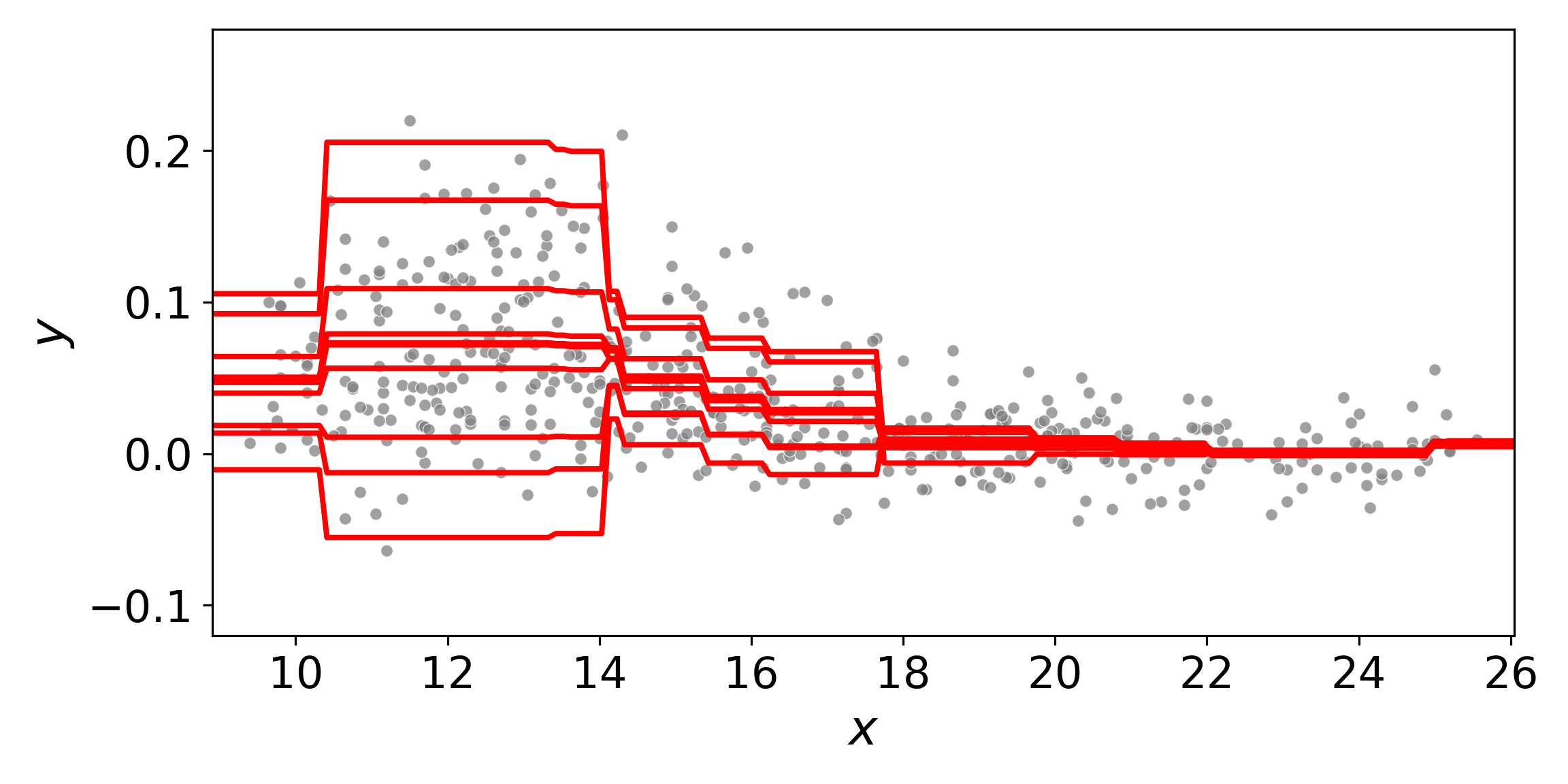
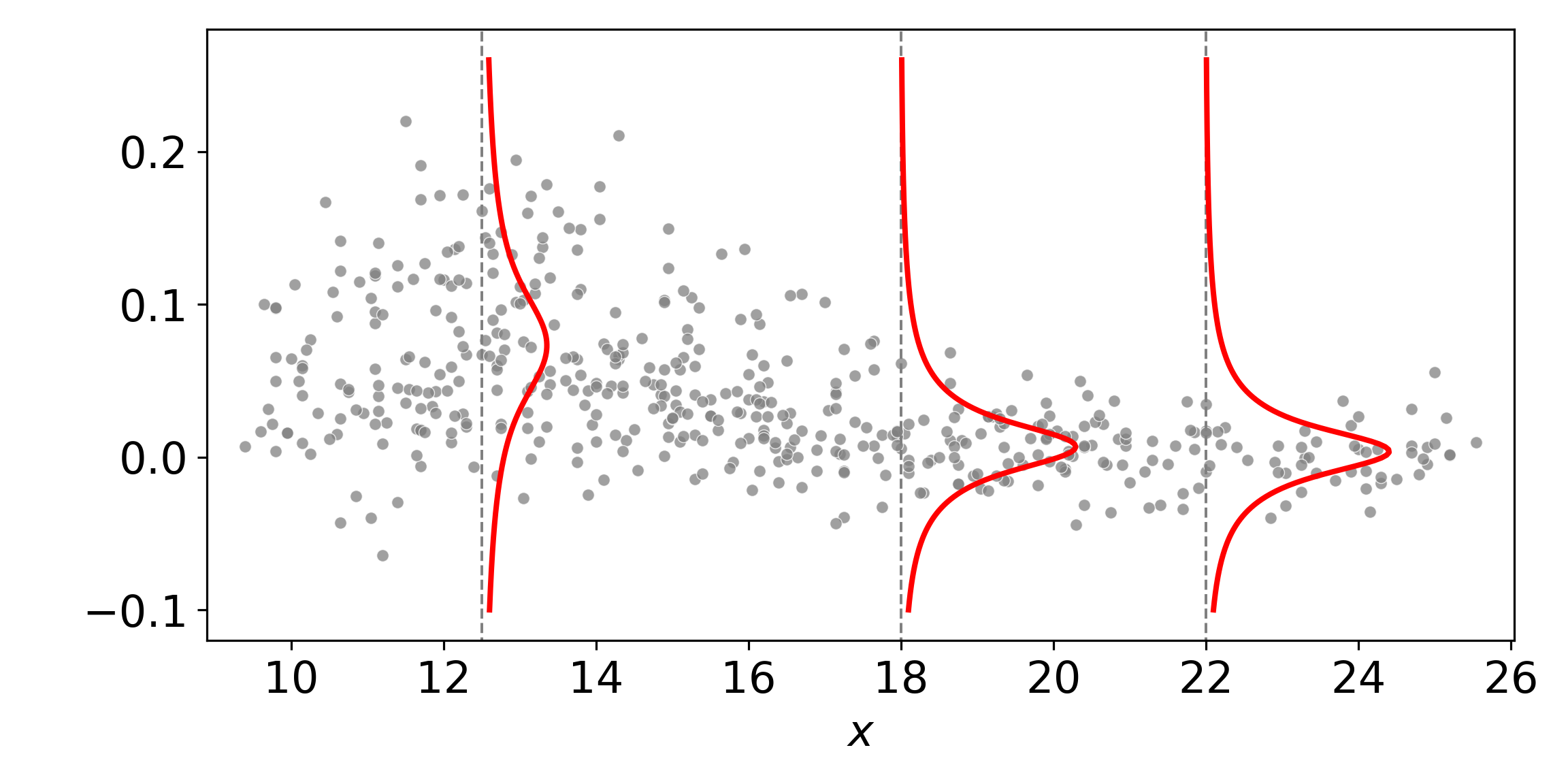
Figure 1: Conditional density estimation for the bone mineral density dataset [21] (grey dots) using WGBoost with a normal output distribution $\mathcal{N}(y\mid m,\sigma)$ placed on the output space $\mathbb{R}$. Left panel: distributional estimate (10 particles) of the location parameter $m$ for each input by WGBoost. Right panel: estimated density based on the normal output distribution averaged over the output particles.

Our Contributions

Our contributions are summarised as follows. First, we provide a general formulation of WGBoost in Section 2. It is a novel family of gradient boosting that returns a set of particles that approximates a target distribution given at each input. In contrast to standard gradient boosting that fits a base learner to the gradient of a loss function, WGBoost fits a base learner to an exactly or approximately available Wasserstein gradient of a loss functional over probability distributions. Second, we develop a concrete algorithm of WGBoost for posterior regression in Section 3, where the loss functional is given by the Kullback–Leibler (KL) divergence of a target posterior. Following modern gradient-boosting libraries [22, 23] that use second-order gradient boosting (c.f. Section 2.2), we establish a second-order WGBoost algorithm built on an approximate Wasserstein gradient and Hessian of the KL divergence. Finally, we demonstrate the performance of regression and classification with OOD detection on real-world tabular datasets in Section 4.

2 General Formulation of Wasserstein Gradient Boosting

This section presents the general formulation of WGBoost. Section 2.1 recaps the notion of Wasserstein gradient flows, a ‘gradient’ system of probability distributions that minimises an objective functional in the Wasserstein space. Section 2.2 recaps the notion of gradient boosting, a sequential ensemble method that fits a new base learner to the ‘gradient’ of the remaining loss. Section 2.3 combines the above two notions to establish a novel family of gradient boosting, WGBoost, whose output is a set of particles that approximates a target distribution assigned at each input.

Notation and Setting  Let $\mathcal{X}$ and $\mathcal{Y}$ be input and output spaces, where a dataset $\{x_{i},y_{i}\}_{i=1}^{D}$ belong. Denote by $\Theta$ the parameter space of an output distribution $p(y\mid\theta)$ on $\mathcal{Y}$. Suppose $\Theta=\mathbb{R}^{d}$ for some dimension $d$ without loss of generality, since re-parametrisation can be performed otherwise. Let $\mathcal{P}_{2}$ be the 2-Wasserstein space, that is, a set of all probability distributions on $\Theta$ with finite second moment equipped with the Wasserstein metric [24]. We identify any probability distribution on $\Theta$ with its density whenever it exits. Denote by $\odot$ and $\oslash$ elementwise multiplication and division of two vectors in $\mathbb{R}^{d}$. Let $\nabla$ be the gradient operator. Let $\nabla_{\text{d}}^{2}$ be a second-order gradient operator that takes the second derivative at each coordinate i.e. $\nabla_{\text{d}}^{2}f(\theta)=[\partial^{2}f(\theta)/\partial\theta_{1}^{2},\dots,\partial^{2}f(\theta)/\partial\theta_{d}^{2}]^{\operatorname{T}}\in\mathbb{R}^{d}$.

2.1 Wasserstein Gradient Flow

In the Euclidean space, a gradient flow of a function $f$ means a curve $x_{t}$ that solves a differential equation $(d/dt)x_{t}=-\nabla f(x_{t})$ from an initial value $x_{0}$. That is the continuous-time limit of gradient descent, which minimises the function $f$ as $t\to\infty$. A Wasserstein gradient flow is a curve of probability distributions $\mu_{t}$ minimising a functional $\mathcal{F}$ on the 2-Wasserstein space $\mathcal{P}_{2}$. The Wasserstein gradient flow $\mu_{t}$ solves a partial differential equation, known as the continuity equation:

$$\frac{d}{dt}\mu_{t}=-\nabla\cdot\left(\mu_{t}\nabla_{W}\mathcal{F}(\mu_{t})\right)\quad\text{given}\quad\mu_{0}\in\mathcal{P}_{2},$$ (1)

where $\nabla_{W}\mathcal{F}(\mu):\Theta\to\Theta$ denotes the Wasserstein gradient of $\mathcal{F}$ at $\mu$ [25, 26]. Appendix A recaps the derivation of the Wasserstein gradient and presents the examples of some functionals.

One of the elegant properties of the Wasserstein gradient flow is casting the infinite-dimensional optimisation of the functional $\mathcal{F}$ as a finite-dimensional particle update [24]. The continuity equation (1) can be reformulated as a dynamical system of a random variable $\theta_{t}\sim\mu_{t}$, such that

$$\frac{d}{dt}\theta_{t}=-\left[\nabla_{W}\mathcal{F}(\mu_{t})\right](\theta_{t})\quad\text{given}\quad\theta_{0}\sim\mu_{0},$$ (2)

in the sense that the law $\mu_{t}$ of the random variable $\theta_{t}$ is a weak solution of the continuity equation. Consider the case where the initial measure is set to the empirical distribution $\hat{\pi}_{0}$ of $N$ particles $\{\theta_{0}^{n}\}_{n=1}^{N}$. Discretising the continuous-time system (2) by the Euler method with a small step size $\nu>0$ yields an iterative update scheme of $N$ particles $\{\theta_{m}^{n}\}_{n=1}^{N}$ from step $m=0$:

$$\begin{bmatrix}\theta_{m+1}^{1}\\ \vdots\\ \theta_{m+1}^{N}\end{bmatrix}=\begin{bmatrix}\theta_{m}^{1}\\ \vdots\\ \theta_{m}^{N}\end{bmatrix}+\nu\begin{bmatrix}-[\nabla_{W}\mathcal{F}(\hat{\pi}_{m})](\theta_{m}^{1})\\ \vdots\\ -[\nabla_{W}\mathcal{F}(\hat{\pi}_{m})](\theta_{m}^{N})\end{bmatrix},$$ (3)

where $\hat{\pi}_{m}$ denotes the empirical distribution of the particles $\{\theta_{m}^{n}\}_{n=1}^{N}$ at step $m$.

In practice, it is common that a chosen functional $\mathcal{F}$ has a Wasserstein gradient that is not well-defined for discrete distributions. In this case, the particle update scheme (3) is not directly applicable because it uses the Wasserstein gradient at the empirical distribution $\hat{\pi}_{m}$. For example, the KL divergence $\mathcal{F}(\mu)=\operatorname{KL}(\mu\mid\pi)$ of a target distribution $\pi$ has a Wasserstein gradient $[\nabla_{W}\mathcal{F}(\mu)](\theta)=-(\nabla\log\pi(\theta)-\nabla\log\mu(\theta))$ that is ill-defined for discrete distributions. One primary approach in such a scenario is to use approximate Wasserstein gradient flows [e.g. 27, 28, 29, 30, 31] that replace the Wasserstein gradient with a certain approximation that is well-defined for discrete distributions. This work uses the ‘smoothed’ Wasserstein gradient of the KL divergence [27] recapped in Section 3.

2.2 Gradient Boosting

Gradient boosting [32] is a sequential ensemble method of $M$ multiple base learners $\{f_{m}\}_{m=1}^{M}$, which iteratively constructs a boosting ensemble of $m$ base learners from step $m=0$ to $M$. Given the current boosting $F_{m}$ at step $m$, it trains a new base learner $f_{m+1}$ to compute the next boosting:

$$F_{m+1}(x)=F_{m}(x)+\nu f_{m+1}(x)$$ (4)

where $\nu$ is a shrinkage hyperparameter called a learning rate. The initial state of the boosting $F_{0}(x)$ at step $m=0$ is set to a constant that best fits the data. Although any learning algorithm can be used as a base learner in principle, tree-based algorithms are most used [33] .

The fundamental idea of gradient boosting is to train the new base learner $f_{m+1}$ to approximate the negative gradient of the remaining error of the current boosting $F_{m}$. Suppose that $\mathcal{Y}=\mathbb{R}^{d}$ and a loss function $L$ measures the remaining error at each data point $R_{i}(F_{m}(x_{i})):=L(F_{m}(x_{i}),y_{i})$. The new base learner $f_{m+1}$ is fitted to the set $\{x_{i},g_{i}\}_{i=1}^{D}$, where the target variable $g_{i}$ is specified as

$$g_{i}=-\nabla R_{i}(F_{m}(x_{i}))\in\mathbb{R}^{d}.$$ (5)

At every input-data point $x_{i}$, the boosting scheme (4) approximately updates the output of the current boosting $F_{m}(x_{i})$ in the steepest descent direction of the error $R_{i}(F_{m}(x_{i}))$. Such an update scheme can be understood as functional gradient descent [34]. Although [32] originally suggested to perform an additional line search to determine a scaling constant for each base learner, it has been reported that the line search can be omitted due to the negligible influence on performance [35].

In modern gradient-boosting libraries e.g. XGBoost [22] and LightGBM [23], the standard practice is to use the diagonal (coordinatewise) Newton direction of the remaining error as the target variable of the new base learner. Let $h_{i}$ be the diagonal of the Hessian matrix of the error:

$$h_{i}:=\nabla_{\text{d}}^{2}R_{i}(F_{m}(x_{i}))\in\mathbb{R}^{d}.$$ (6)

The new base leaner $f_{m+1}$ is fitted to the set $\{x_{i},g_{i}\oslash h_{i}\}_{i=1}^{n}$, where the negative gradient $g_{i}$ is divided elementwise by the Hessian diagonal $h_{i}$. The target variable $g_{i}\oslash h_{i}$ is the diagonal Newton direction that minimises the second-order Taylor approximation of the remaining error for each coordinate independently. Combining this second-order gradient boosting and tree-based algorithms has demonstrated exceptional scalability and performance [36, 37]. Although it is possible to use the ‘full’ Newton direction as the target variable, the impracticality of the full Newton direction has been pointed out [e.g. 38, 39], and the coordinatewise computability of the diagonal Newton direction is suitable for many of popular gradient-boosting tree algorithms [38].

2.3 Wasserstein Gradient Boosting

Suppose that we are given a loss functional $\mathcal{F}_{i}(\mu)$ over probability distributions $\mu\in\mathcal{P}_{2}$ on $\Theta$ at each input-data point $x_{i}$. For example, the loss functional can be specified by some divergence $\mathcal{F}_{i}(\mu)=\operatorname{D}(\mu\mid\pi_{i})$—such as the KL divergence—of a target distribution $\pi_{i}$ assigned at each $x_{i}$. Given the inputs and loss functionals $\{x_{i},\mathcal{F}_{i}\}_{i=1}^{D}$, our aim is to construct a map from an input to $N$ particles in $\Theta$ whose empirical distribution approximately minimises the loss functional $\mathcal{F}_{i}$. Our approach is to combine gradient boosting with Wasserstein gradient, where we sequentially construct a set of $N$ boostings $\{F_{m}^{n}\}_{n=1}^{N}$—each of which consists of $m$ base learners—from step $m=0$.

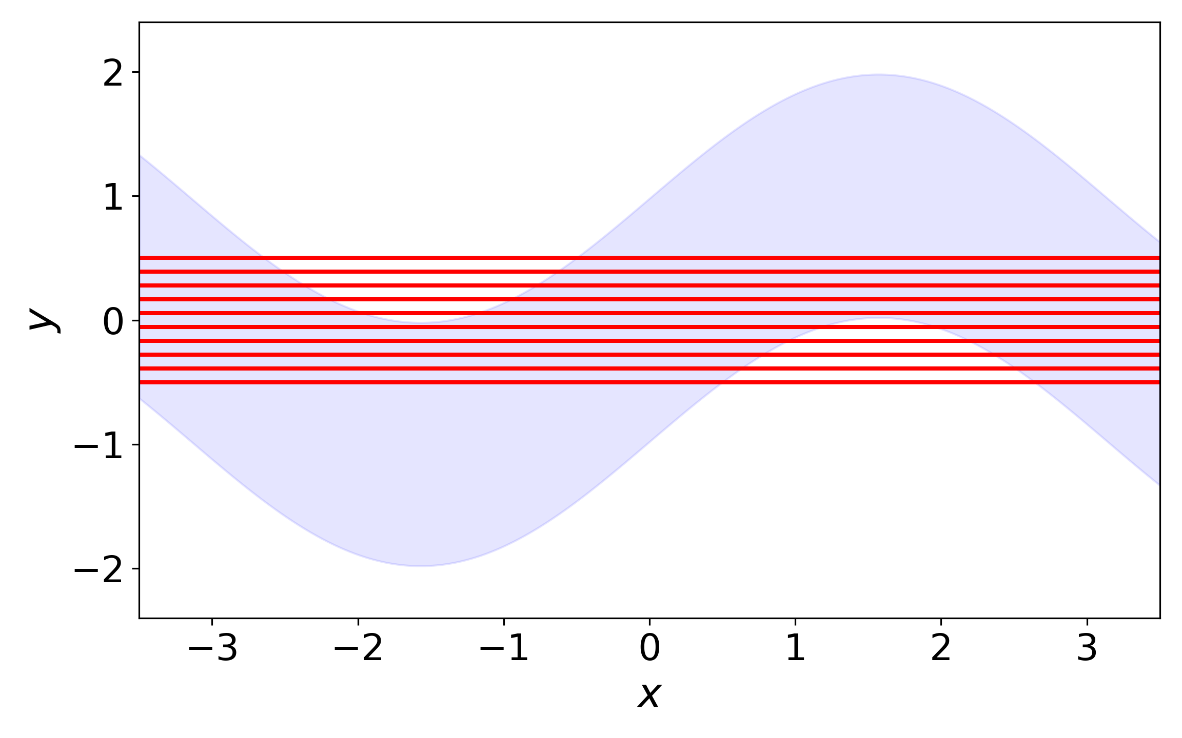
(a) $0$% trained

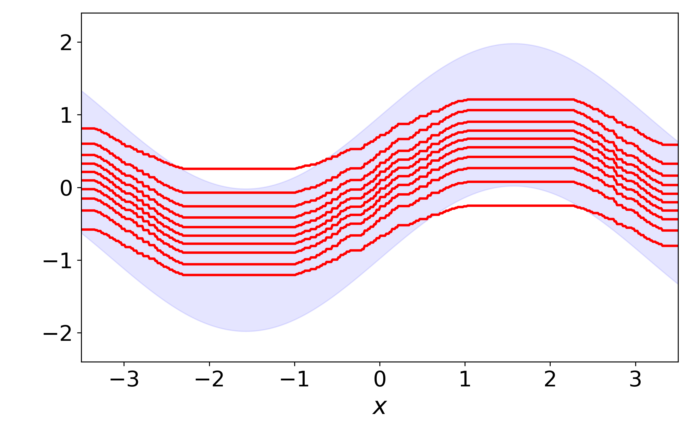
(b) $15$% trained

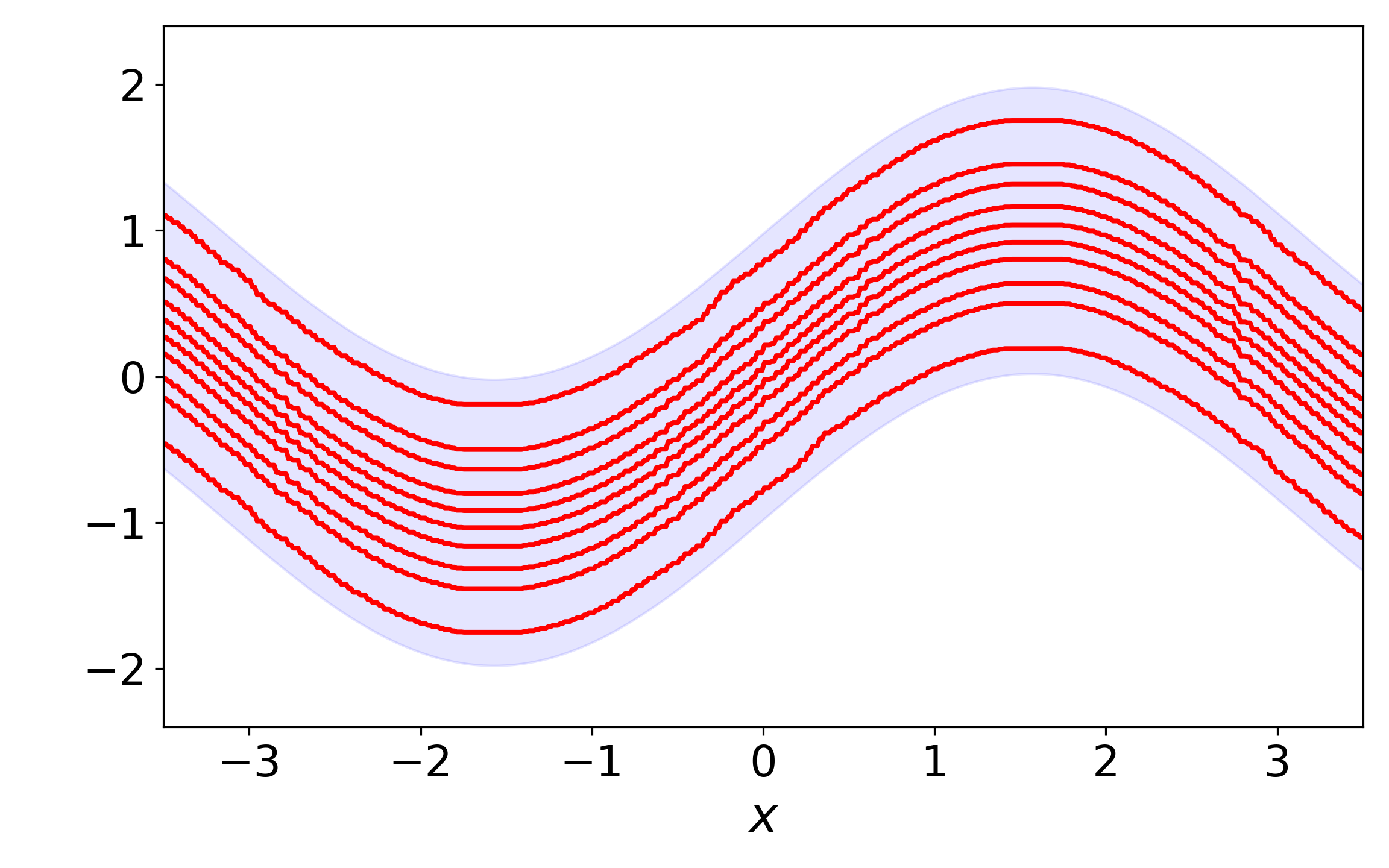
(c) $100$% trained

Figure 2: Illustration of the WGBoost output, where the target distribution is $\mathcal{N}(\theta\mid\sin(x),0.5)$ at each input $x$, and the base learner is the decision tree regressor [40]. The blue area indicates the $95$% high probability region of the target. Panel (a): initial $10$ output particles of WGBoost. Panel (b) and (c): updated output particles of WGBoost with $15$ and $100$ base learners trained, respectively.

Here, each $n$-th boosting $F_{m}^{n}$ is a map from $\mathcal{X}$ to $\Theta$ at any step $m$. Its output $F_{m}^{n}(x)$ represents the $n$-th output particle for each input $x$. Given the current set of $N$ boostings $\{F_{m}^{n}\}_{n=1}^{N}$ at step $m$, WGBoost trains a set of $N$ new base learners $\{f_{m+1}^{n}\}_{n=1}^{N}$ and computes the next set of $N$ boostings:

$$\begin{bmatrix}F_{m+1}^{1}(x)\\ \vdots\\ F_{m+1}^{N}(x)\end{bmatrix}=\begin{bmatrix}F_{m}^{1}(x)\\ \vdots\\ F_{m}^{N}(x)\end{bmatrix}+\nu\begin{bmatrix}f_{m+1}^{1}(x)\\ \vdots\\ f_{m+1}^{N}(x)\end{bmatrix}$$ (7)

where $\nu$ is a learning rate. Similarly to standard gradient boosting, the initial state of the set of $N$ boostings $\{F_{0}^{n}\}_{n=1}^{N}$ at step $m=0$ is set to a given set of constants. Throughout, let $\hat{\pi}_{m}(x)$ denote the empirical distribution of the $N$ output particles $\{F_{m}^{n}(x)\}_{n=1}^{N}$ at step $m$ for each input $x$.

For better presentation, let $\mathcal{G}_{i}(\mu)$ denote the Wasserstein gradient of each loss functional $\mathcal{F}_{i}(\mu)$. The foundamental idea of WGBoost is to train the $n$-th new learner $f_{m+1}^{n}$ to approximate the negative Wasserstein gradient $-\mathcal{G}_{i}(\hat{\pi}_{m}(x_{i}))$ evaluated at the $n$-th boosting output $F_{m}^{n}(x_{i})$ for each $x_{i}$, so that

$$\begin{bmatrix}f_{m+1}^{1}(x_{i})\\ \vdots\\ f_{m+1}^{N}(x_{i})\end{bmatrix}\approx\begin{bmatrix}-\left[\mathcal{G}_{i}\left(\hat{\pi}_{m}(x_{i})\right)\right]\left(F_{m}^{1}(x_{i})\right)\\ \vdots\\ -\left[\mathcal{G}_{i}\left(\hat{\pi}_{m}(x_{i})\right)\right]\left(F_{m}^{N}(x_{i})\right)\end{bmatrix}.$$ (8)

At every input-data point $x_{i}$, the boosting scheme (7) approximates the particle update scheme (3) for the output particles $\{F_{m}^{n}(x_{i})\}_{n=1}^{N}$ under the Wasserstein gradint $\mathcal{G}_{i}(\hat{\pi}_{m}(x_{i}))=\nabla_{W}\mathcal{F}_{i}(\hat{\pi}_{m}(x_{i}))$, by which each boosting output is updated in the direction to decrease the loss functional. As stated in Section 2.1, some loss functionals have a Wasserstein gradient that is not well-defined for empirical distributions. Any suitable approximation of the Wasserstein gradient can be used as $\mathcal{G}_{i}(\mu)$, which results in an approximate WGBoost, as in approximate Wasserstein gradient flows.

The general procedure of exact or approximate WGBoost is summarised in Algorithm 1. Similarly to standard gradient boosting, various loss functionals may lead to a different WGBoost. Appendix A presents examples of Wasserstein gradients of common divergences. Figure 2 illustrates the output of WGBoost using a simple target distribution $\pi_{i}(\theta)=\mathcal{N}(\theta\mid\sin(x_{i}),0.5)$ when the approximate Wasserstein gradient of the KL divergence presented later in (12) is applied as $\mathcal{G}_{i}$ in Algorithm 1.

Data: set $\{x_{i},\mathcal{F}_{i}\}_{i=1}^{D}$ of input $x_{i}$ and loss functional $\mathcal{F}_{i}$

Input: exact or approximate Wasserstein gradient $\mathcal{G}_{i}(\mu)$ of loss functional $\mathcal{F}_{i}(\mu)$, particle number $N$, iteration $M$, learning rate $\eta$, learning algorithm $f$, initial constants $\{\vartheta_{0}^{n}\}_{n=1}^{N}$

Output: set of $N$ boostings $\{F_{M}^{n}\}_{n=1}^{N}$

for $n\leftarrow 1,\dots,N$ do

       $F_{0}^{n}(\cdot)\leftarrow\vartheta_{0}^{n}$ $\rhd$ set initial state of $n$-th boosting

end for

for $m\leftarrow 0,\dots,M-1$ do

       for $n\leftarrow 1,\dots,N$ do

             for $i\leftarrow 1,\dots,D$ do

                   $g_{i}^{n}\leftarrow-\left[\mathcal{G}_{i}(\hat{\pi}_{m}(x_{i}))\right]\left(F_{m}^{n}(x_{i})\right)$ $\rhd$ Wasserstein gradient of $n$-th boosting

             end for

            $f_{m+1}^{n}\leftarrow\text{fit}\left(\left\{x_{i},g_{i}^{n}\right\}_{i=1}^{D}\right)$ $\rhd$ fit new base learner of $n$-th boosting

             $F_{m+1}^{n}(\cdot)\leftarrow F_{m}^{n}(\cdot)+\nu f_{m+1}^{n}(\cdot)$ $\rhd$ get next state of $n$-th boosting

       end for

      

end for

Algorithm 1 Wasserstein Gradient Boosting

Remark 1 (Stochastic WGBoost).

Stochastic gradient boosting [41] uses only a randomly sampled subset of data to fit a new base learner at each step $m$ to reduce the computational cost. The same subsampling approach can be applied for WGBoost whenever the dataset is large.

Remark 2 (Second-Order WGBoost).

If a loss functional $\mathcal{F}_{i}$ admits an exactly or approximately available Wasserstein ‘Hessian’, the associated Newton direction may also be computable [e.g. 42, 43]. Implementing a second-order WGBoost algorithm is immediately possible by plugging such a Newton direction into $\mathcal{G}_{i}(\mu)$ in Algorithm 1. The default WGBoost algorithm for posterior regression is built on a diagonal approximate Wasserstein Newton direction of the KL divergence, aligning with the standard practice in modern gradient-boosting libraries to use the diagonal Newton direction.

3 Default Implementation for Posterior Regression under KL Divergence

This section provides the default setting to implement a concrete WGBoost algorithm for posterior regression, where each loss functional $\mathcal{F}_{i}(\mu)$ is specified by the KL divergence of a target posterior. Section 3.1 recaps the definition of the target posterior in posterior regression, followed by the default choice of the prior discussed in Section 3.2. Section 3.3 recaps a widely-used approximate Wasserstein gradient of the KL divergence based on kernel smoothing [27]. A further advantage of the kernel smoothing approach is that the approximate Wasserstein Hessian is available. Section 3.4 establishes a second-order WGBoost algorithm, similarly to modern gradient-boosting libraries.

3.1 Target Posterior

Suppose that a parametric output distribution $p(y\mid\theta)$ is specified on the output space $\mathcal{Y}$ as is often done in most probabilistic prediction methods. Suppose further that a prior distribution $p_{i}(\theta)$ of the output-distribution parameter $\theta$ is specified at each data point $(x_{i},y_{i})$ in the dataset. At each data point $(x_{i},y_{i})$, the likelihood $p(y_{i}\mid\theta)$ and the prior $p_{i}(\theta)$ determine the posterior distribution:

$$\pi_{i}(\theta)\propto p(y_{i}\mid\theta)p_{i}(\theta).$$ (9)

In posterior regression, the target variable is the posterior distribution $\pi_{i}$ assigned pointwise at each input-data point $x_{i}$ We apply the framework of WGBoost to construct a map from an input to a set of particles that approximates each target posterior $\pi_{i}$ under the loss functional $\mathcal{F}_{i}(\mu)=\operatorname{KL}(\mu\mid\pi_{i})$.

The constructed map can produce a distributional estimate of the output-distribution parameter $\theta$ for a new input $x$. Recall that $\hat{\pi}_{M}(x)$ denotes the empirical distribution of the output particles of WGBoost at the final step $M$ for each input $x$. Based on the output particles of WGBoost, a predictive distribution $p(y\mid x)$ is defined for each input $x$ via the Bayesian model averaging:

$$p(y\mid x)=\mathbb{E}_{\theta\sim\hat{\pi}_{M}(x)}\left[p\left(y\mid\theta\right)\right].$$ (10)

A point prediction $\hat{y}$ can also be defined for each input $x$ via the Bayes action:

$$\hat{y}=\text{argmin}_{y\in\mathcal{Y}}~{}\mathbb{E}_{\theta\sim\hat{\pi}_{M}(x)}\left[U(y,\theta)\right],$$ (11)

which is the minimiser of the average risk of a given utility $U:\mathcal{Y}\times\Theta\to\mathbb{R}$. For example, if the utility is a quadratic function $U(y,\theta)=(y-\theta)^{2}$, the Bayes action is the mean value of $\hat{\pi}_{M}(x)$.

In general, the explicit form of the posterior $\pi_{i}$ is known only up to the normalising constant. The WGBoost algorithm for posterior regression, provided in Section 3.4, requires no normalising constant of the posterior $\pi_{i}$. It depends only on the log-gradient of the posterior $\nabla\log\pi_{i}(\theta)=\nabla\pi_{i}(\theta)/\pi_{i}(\theta)$ and the diagonal of the log-Hessian of the posterior, cancelling the normalising constant by fraction. Hence, knowing the form of the likelihood $p(y_{i}\mid\theta)$ and prior $p_{i}(\theta)$ suffices.

3.2 Choice of Prior

In posterior regression, the prior $p_{i}(\theta)$ of the output-distribution parameter $\theta$ is specified at each data point $(x_{i},y_{i})$. The approach to specifying the prior may differ depending on whether past data are available. When past data are available, they can be utilised in any possible way to elicit a reasonable prior for future data. When no past data are available, we recommend the use of a noninformative prior; see [e.g. 44] for the introduction of noninformative priors that have been developed as a sensible choice of prior in the absence of past data. Precisely, in order to avoid numerical errors, if a noninformative prior is improper (nonintegrable) as is often the case, we recommend the use of a proper probability distribution that approximates the noninformative prior sufficiently well.

Example 1 (Normal Location-Scale).

A normal location-scale distribution $\mathcal{N}(y\mid m,\sigma)$ of a scalar output $y\in\mathbb{R}$ has the mean and scale parameters $m\in\mathbb{R}$ and $\sigma\in(0,\infty)$. A typical noninformative prior of $m$ and $\sigma$ is each given by $1$ and $1/\sigma$, which are improper. At every data point $(x_{i},y_{i})$, we use a normal prior $\mathcal{N}(m\mid 0,\sigma_{0})$ over $m$ and an inverse gamma prior $\operatorname{IG}(\sigma\mid\alpha_{0},\beta_{0})$ over $\sigma$, with the hyperparameters $\sigma_{0}=10$ and $\alpha_{0}=\beta_{0}=0.01$, which approximate the non-informative priors.

Example 2 (Categorical).

A categorical distribution $\mathcal{C}(y\mid q)$ of a $k$-class label $y\in\{1,\dots,k\}$ has a class probability parameter $q=(q_{1},\dots,q_{k})$ in the $k$-dimensional simplex $\Delta_{k}$. It corresponds to the Bernoulli distribution if $k=2$. A typical noninformative prior of $q$ is given by $1/(q_{1}\times\dots\times q_{k})$. At every data point $(x_{i},y_{i})$, we use the logistic normal prior—a multivariate generalisation of the logit normal distribution [45]—over $q$ with the mean $0$ and identity covariance matrix scaled by $10$.

In Section 2, $\Theta=\mathbb{R}^{d}$ is supposed for some dimension $d$, as any parameter that lies in a subset of the Euclidean space (e.g. $\sigma$) can be reparametrised as one in the Euclidean space (e.g. $\log\sigma$). Appendix E details the reparametrisation used for the experiment. When a dataset has scalar outputs of a low or high order of magnitude, we also recommend to standardise the outputs to adjust the magnitude.

3.3 Approximate Wasserstein Gradient of KL Divergence

The loss functional $\mathcal{F}_{i}(\mu)$ considered for posterior regression is the KL divergence $\operatorname{KL}(\mu\mid\pi_{i})$. A computational challenge of the KL divergence is that the associated Wasserstein gradient $\left[\mathcal{G}_{i}^{\text{KL}}(\mu)\right](\theta):=-\left(\nabla\log\pi_{i}(\theta)-\nabla\log\mu(\theta)\right)$ is not well-defined for empirical distributions. A particularly successful approach to finding a well-defined approximation of the Wasserstein gradient—which originates in [46] and has been applied in wide contexts [27, 47, 48]—is to smooth the original Wasserstein gradient through a kernel integral operator $\int_{\Theta}[\mathcal{G}_{i}^{\text{KL}}(\mu)](\theta^{*})k(\theta,\theta^{*})d\mu(\theta^{*})$ [49]. By integration-by-part (see [e.g. 46]), the smoothed Wasserstein gradient, denoted $\mathcal{G}^{*}_{i}(\mu)$, falls into the following form that is well-defined for any probability distribution $\mu$:

$$\left[\mathcal{G}^{*}_{i}(\mu)\right](\theta) :=-\mathbb{E}_{\theta^{*}\sim\mu}\Big{[}\nabla\log\pi_{i}(\theta^{*})k(\theta,\theta^{*})+\nabla k(\theta,\theta^{*})\Big{]}\in\mathbb{R}^{d},$$ (12)

where $\nabla k(\theta,\theta^{*})$ denotes the gradient of $k$ with respect to the first argument $\theta$. An approximate Wasserstein gradient flow based on the smoothed Wasserstein gradient $\mathcal{G}^{*}_{i}(\mu)$ is called the Stein variational gradient descent [46] or kernelised Wasserstein gradient flow [50]. In most cases, the kernel $k$ is set to the Gaussian kernel $k(\theta,\theta^{*})=\exp(-\|\theta-\theta^{*}\|^{2}/h)$ with the scale hyperparameter $h>0$. We use the Gaussian kernel with the scale hyperparameter $h=0.1$ throughout this work.

Another common approach to approximating the Wasserstein gradient flow of the KL divergence is the Langevin diffusion approach [51]. The discretised algorithm, called the unadjusted Langevin algorithm [52], is a stochastic particle update scheme that adds a Gaussian noise at every iteration. However, several known challenges, such as asymptotic bias and slow convergence, often necessitate an ad-hoc adjustment of the algorithm [51]. Appendix B discusses a variant of WGBoost built on the Langevin algorithm, although it is not considered the default implementation.

3.4 Default Second-Order Implementation of WGBoost

Following the standard practice in modern gradient-boosting libraries [22, 23] to use the diagonal Newton direction, we further consider a diagonal (coordinatewise) approximate Wasserstein Newton direction of the KL divergence. In a similar manner to the smoothed Wasserstein gradient (12), the approximate Wasserstein Hessian of each KL divergence $\operatorname{KL}(\mu\mid\pi_{i})$ can be obtained by the kernel smoothing. The diagonal of the approximate Wasserstein Hessian, denoted $\mathcal{H}_{i}^{*}(\mu)$, is defined by

$$\left[\mathcal{H}_{i}^{*}(\mu)\right](\theta):=\mathbb{E}_{\theta^{*}\sim\mu}\Big{[}-\nabla_{\text{d}}^{2}\log\pi_{i}(\theta^{*})k(\theta,\theta^{*})^{2}+\nabla k(\theta,\theta^{*})\odot\nabla k(\theta,\theta^{*})\Big{]}\in\mathbb{R}^{d}.$$ (13)

The diagonal approximate Wasserstein Newton direction of each KL divergence is then defined by $-\left[\mathcal{G}_{i}^{*}(\mu)\right](\cdot)\oslash\left[\mathcal{H}_{i}^{*}(\mu)\right](\cdot)$. Appendix C provides the derivation based on [42] who derived the Newton direction of the KL divergence in the context of nonparametric variational inference. The second-order WGBoost algorithm is established by plugging it into $\mathcal{G}_{i}(\mu)$ in Algorithm 1 i.e.

$$\left[\mathcal{G}_{i}(\mu)\right](\cdot)=\left[\mathcal{G}_{i}^{*}(\mu)\right](\cdot)\oslash\left[\mathcal{H}_{i}^{*}(\mu)\right](\cdot).$$ (14)

Algorithm 1 under the setting (14) is considered our default WGBoost algorithm for posterior regression. We refer the algorithm to as second-order KL approximate WGBoost (SKA-WGBoost). For full clarity, the explicit pseudocode is provided in Appendix D.

Although it is possible to use the full Newton direction with no diagonal approximation, the inverse and product of $(N\times d)\times(N\times d)$ matrices are required at every computation of the direction (c.f. Appendix E), which can be a computational bottleneck if the size of data or output particles is large. The diagonal Newton direction has a clear computational benefit in that only elementwise division is involved. The computational complexity is the same as that for the smoothed Wasserstein gradient, scaling linearly to both the particle number $N$ and the parameter dimension $d$. Hence, there is essentially no reason not to use the diagonal Newton direction instead of the smoothed Wasserstein gradient. Appendix E presents a simulation study to compare different WGBoost algorithms.

4 Applications with Real-world Tabular Data

We empirically demonstrate the performance of the default WGBoost algorithm, SKA-WGBoost, through three applications using real-world tabular data. The first application illustrates the output of the WGBoost algorithm through a simple conditional density estimation. The second application benchmarks the regression performance on nine real-world datasets [53]. The third application examines the classification and OOD detection performance on the real-world datasets used in [14].

Throughout, in SKA-WGBoost, we set the number of output particles $N$ to $10$ and set each base learner $f$ to the decision tree regressor [40] with maximum depth $1$ for the first application and $3$ for the rest. Appendix F contains further details, including a choice of the initial constant $\{\vartheta_{0}^{n}\}_{n=1}^{N}$. The source code is available in https://github.com/takuomatsubara/WGBoost.

4.1 Illustrative Conditional Density Estimation

This section illustrates the output of the WGBoost algorithm by estimating a conditional density $p(y\mid x)$ from one-dimensional scalar inputs and outputs $\{x_{i},y_{i}\}_{i=1}^{D}$. The normal output distribution $\mathcal{N}(y\mid m,\sigma)$ and the prior $p_{i}(m,\sigma)$ in Example 1 were used, where the output of the WGBoost algorithm is a set of $10$ particles $\{(m^{n},\sigma^{n})\}_{n=1}^{10}$ of the mean and scale parameters $(m,\sigma)$ for each input $x$. We set the number of base learners $M$ to $500$ and the learning rate $\nu$ to $0.1$. The conditional density is estimated using the predictive distribution (10) by the WGBoost algorithm. We used two real-world datasets, bone mineral density [21] and old faithful geyser [54]. Figure 1 depicts the result for the former dataset, demonstrating that the WGBoost algorithm captures the heterogeneity of the conditional density on each input well. Appendix F presents the result for the latter dataset.

Table 1: NLLs (a) and RMSEs (b) of the six probabilistic regression algorithms with the standard deviation. The best score is underlined for each dataset, and the scores whose standard deviation ranges include the best score are in bold. Results of MCDropout, DEnsembles, CDropout, NGBoost, and DEvidential were reported in [9], [10], [55], [33] and [13] respectively.

(a) NLLs of the predictive distributions

Dataset	WGBoost	MCDropout	DEnsemble	CDropout	NGBoost	DEvidential
boston	2.47 ± 0.16	2.46 ± 0.06	2.41 ± 0.25	2.72 ± 0.01	2.43 ± 0.15	2.35 ± 0.06
concrete	2.83 ± 0.11	3.04 ± 0.02	3.06 ± 0.18	3.51 ± 0.00	3.04 ± 0.17	3.01 ± 0.02
energy	0.53 ± 0.08	1.99 ± 0.02	1.38 ± 0.22	2.30 ± 0.00	0.60 ± 0.45	1.39 ± 0.06
kin8nm	-0.44 ± 0.03	-0.95 ± 0.01	-1.20 ± 0.02	-0.65 ± 0.00	-0.49 ± 0.02	-1.24 ± 0.01
naval	-5.47 ± 0.03	-3.80 ± 0.01	-5.63 ± 0.05	-5.87 ± 0.05	-5.34 ± 0.04	-5.73 ± 0.07
power	2.60 ± 0.04	2.80 ± 0.01	2.79 ± 0.04	2.75 ± 0.01	2.79 ± 0.11	2.81 ± 0.07
protein	2.70 ± 0.01	2.89 ± 0.00	2.83 ± 0.02	2.81 ± 0.00	2.81 ± 0.03	2.63 ± 0.00
wine	0.95 ± 0.08	0.93 ± 0.01	0.94 ± 0.12	1.70 ± 0.00	0.91 ± 0.06	0.89 ± 0.05
yacht	0.16 ± 0.24	1.55 ± 0.03	1.18 ± 0.21	1.75 ± 0.00	0.20 ± 0.26	1.03 ± 0.19

(b) RMSEs of the point predictions

Dataset	WGBoost	MCDropout	DEnsemble	CDropout	NGBoost	DEvidential
boston	2.78 ± 0.60	2.97 ± 0.19	3.28 ± 1.00	2.65 ± 0.17	2.94 ± 0.53	3.06 ± 0.16
concrete	4.15 ± 0.52	5.23 ± 0.12	6.03 ± 0.58	4.46 ± 0.16	5.06 ± 0.61	5.85 ± 0.15
energy	0.42 ± 0.07	1.66 ± 0.04	2.09 ± 0.29	0.46 ± 0.02	0.46 ± 0.06	2.06 ± 0.10
kin8nm	0.15 ± 0.00	0.10 ± 0.00	0.09 ± 0.00	0.07 ± 0.00	0.16 ± 0.00	0.09 ± 0.00
naval	0.00 ± 0.00	0.01 ± 0.00	0.00 ± 0.00	0.00 ± 0.00	0.00 ± 0.00	0.00 ± 0.00
power	3.19 ± 0.25	4.02 ± 0.04	4.11 ± 0.17	3.70 ± 0.04	3.79 ± 0.18	4.23 ± 0.09
protein	4.09 ± 0.02	4.36 ± 0.01	4.71 ± 0.06	3.85 ± 0.02	4.33 ± 0.03	4.64 ± 0.03
wine	0.61 ± 0.05	0.62 ± 0.01	0.64 ± 0.04	0.62 ± 0.00	0.63 ± 0.04	0.61 ± 0.02
yacht	0.48 ± 0.18	1.11 ± 0.09	1.58 ± 0.48	0.57 ± 0.05	0.50 ± 0.20	1.57 ± 0.56

4.2 Probabilistic Regression Benchmark

This section examines the regression performance of the WGBoost algorithm using a widely-used benchmark protocol that originated in [53] and has been used in subsequent work [10, 9, 33]. We used nine real-world tabular datasets from the University of California Irvine machine learning repository [56], each with one-dimensional scalar outputs. As in Section 4.1, the normal output distribution $\mathcal{N}(y\mid m,\sigma)$ and the prior $p_{i}(m,\sigma)$ in Example 1 were used. We randomly held out 10% of each dataset as a test set to measure the negative log likelihood (NLL) of the predictive distribution (10) by the WGBoost algorithm and the room mean squared error (RMSE) of the point prediction produced by taking the mean value of the predictive distribution. We chose the number of base learners $M$ using an early-stopping approach, following [33], where we held out 20% of the training set as a validation set to choose the number $1\leq M\leq 4000$ achieving the least validation error. Once the number $M$ was chosen, the WGBoost algorithm was trained again using all the entire training set. We set the learning rate $\nu$ to $0.1$ for all the nine datasets. We repeated this procedure 20 times for each dataset, except the protein dataset for which we repeated five times.

We compared the performance of the WGBoost algorithm with five other methods: Monte Carlo Dropout (MCDropout) [9], Deep Ensemble (DEnsemble) [10], Concrete Dropout (CDropout) [55], Natural Gradient Boosting (NGBoost) [33], and Deep Evidential Regression (DEvidential) [13]. Appendix F briefly describes each algorithm and provides further details on the experiment. Table 1 summarises the NLLs and RMSEs of the six algorithms. The WGBoost algorithm achieves the best score or a score sufficiently close to the best score for the majority of the nine datasets.

4.3 Classification and Out-of-Distribution Detection

This section examines the classification and anomaly OOD detection performance of the WGBoost algorithm on two real-world tabular datasets, segment and sensorless, following the protocol used in [14]. The categorical output distribution $\mathcal{C}(y\mid q)$ and the prior $p_{i}(q)$ in Example 2 were used, where the output of the WGBoost algorithm is a set of $10$ particles $\{q^{n}\}_{n=1}^{10}$ of the class probability parameter $q$ in the simplex $\Delta^{k}$ for each input $x$. We set the number of base learners $M$ to $4000$ and the learning rate $\nu$ to $0.4$. The dispersion of the output particles of the WGBoost algorithm was used for OOD detection [57]. If a test input was an in-distribution sample from the same distribution as the data, we expected the output particles to concentrate on some small region in $\Delta^{k}$ indicating a high probability of the correct class. If a test input was an OOD sample, we expected the output particles to disperse over $\Delta^{k}$ because the model ought to be less certain about the correct class.

The segment and sensorless datasets have 7 and 11 classes in total. For the segment dataset, the data subset that belongs to the last class was kept as the OOD samples. For the sensorless dataset, the data subset that belongs to the last two classes was kept as the OOD samples. For each dataset, 20% of the non-OOD samples is held out as a test set to measure the classification accuracy. Several approaches can define the OOD score of each input [57]. We focused on an approach that uses the variance of the output particles as the OOD score. For the WGBoost algorithm, we employed the inverse of the maximum norm of the variance as the OOD score. Given the OOD score, we measured the OOD detection performance by the area under the precision recall curve (PR-AUC), viewing non-OOD test data as the positive class and OOD data as the negative class. We repeated this procedure five times.

Table 2: Classification accuracies and OOD detection PR-AUCs of the five algorithms with the standard deviation, scaled in $[0,100]$. For each dataset, the best score is underlined and in bold. The results of the other algorithms than the WGBoost algorithm were reported in [14].

Dataset	Criteria	WGBoost	MCDropout	DEnsemble	DDistillation	PNetwork
segment	Accuracy	96.57 ± 0.6	95.25 ± 0.1	97.27 ± 0.1	96.21 ± 0.1	96.92 ± 0.1
	OOD	99.67 ± 0.2	43.11 ± 0.6	58.13 ± 1.7	35.83 ± 0.4	96.74 ± 0.9
sensorless	Accuracy	99.54 ± 0.1	89.32 ± 0.2	99.37 ± 0.0	93.66 ± 1.5	99.52 ± 0.0
	OOD	81.13 ± 5.3	40.61 ± 0.7	50.62 ± 0.1	31.17 ± 0.2	88.65 ± 0.4

We compared the WGBoost algorithm with four other methods: MCDropout, DEnsemble, and Distributional Distillation (DDistillation) [58], and Posterior Network (PNetwork) [14]. Appendix F briefly describes each algorithm and provides further details on the experiment. Table 2 summarises the classification and OOD detection performance of the five algorithms. The WGBoost algorithm demonstrates a high classification and OOD detection accuracy simultaneously. Although PNetwork has the best OOD detection performance for the sensorless dataset, the performance of the WGBoost algorithm also exceeds 80%, which is distinct from MCDropout, DEnsemble, and DDistillation.

5 Discussion

We proposed a general framework of WGBoost. We further established a second-order WGBoost algorithm for posterior regression, aligning with the standard practice in modern gradient-boosting libraries. We empirically demonstrated that the probabilistic forecast by WGBoost leads to better predictive accuracy and OOD detection performance. This work offers exciting avenues for future research. Important directions for future study include investigating the convergence properties, evaluating the robustness to misspecified output distributions, and exploring alternatives to the KL divergence. One limitation of WGBoost may arise when data are not tabular, as in the case of standard gradient boosting. These questions require careful examination and are critical for future work.

Appendix

This appendix contains the technical and experiment details referred to in the main text. Appendix A recaps the derivation of the Wasserstein gradient and presents several examples. Appendix B discusses a variant of WGBoost for the KL divergence built on the unadjusted Langevin algorithm. Appendix C derives the diagonal approximate Wasserstein Newton direction used for the default WGBoost algorithm, SKA-WGBoost. Appendix D shows the explicit pseudocode of SKA-WGBoost for full clarify. Appendix E provides a simulation study to compare four different WGBoost algorithms. Appendix F describes the additional details of the experiment in the main text.

Appendix A Derivation and Example of Wasserstein Gradient

This section recaps the derivation of the Wasserstein gradient of a functional $\mathcal{F}$, with examples of common divergences. The Wasserstein gradient depends on a function on $\Theta$ called the first variation [25]. The first variation $\delta\mathcal{F}(\mu)/\delta\mu$ of the functional $\mathcal{F}$ at $\mu$ is a function on $\Theta$ that satisfies

$$\lim_{\epsilon\to 0^{+}}\frac{\mathcal{F}(\mu+\epsilon\nu)-\mathcal{F}(\mu)}{\epsilon}=\int_{\Theta}\frac{\delta\mathcal{F}(\mu)}{\delta\mu}(\theta)\nu(\theta)d\theta$$ (15)

for all signed measure $\nu$ s.t. $\mu+\epsilon\nu\in\mathcal{P}_{2}$ for all $\epsilon$ sufficiently small. The Wasserstein gradient $\nabla_{W}\mathcal{F}(\mu)$ of the functional $\mathcal{F}$ at $\mu$ is derived as the gradient of the first variation (see [e.g. 25]):

$$[\nabla_{W}\mathcal{F}(\mu)](\theta):=\nabla\frac{\delta\mathcal{F}(\mu)}{\delta\mu}(\theta).$$ (16)

It is common to suppose that the functional $\mathcal{F}$ consists of three energies, which are determined by functions $U:\mathbb{R}\to\mathbb{R}$, $V:\Theta\to\mathbb{R}$, and $W:\Theta\to\mathbb{R}$ respectively, such that

$$\mathcal{F}(\mu)=\underbrace{\int_{\Theta}U(\mu(\theta))d\theta}_{\text{internal energy}}+\underbrace{\int_{\Theta}V(\theta)\mu(\theta)d\theta}_{\text{potential energy}}+\underbrace{\frac{1}{2}\int_{\Theta\times\Theta}W(\theta-\theta^{\prime})\mu(\theta)d\theta\mu(\theta^{\prime})d\theta^{\prime}}_{\text{interaction energy}}.$$ (17)

For a functional $\mathcal{F}$ that falls into the above form, the Wasserstein gradient is derived as

$$\left[\nabla_{W}\mathcal{F}(\mu)\right](\theta)=\nabla U^{\prime}(\mu(\theta))+\nabla V(\theta)+\int_{\Theta}\nabla W(\theta-\theta^{\prime})\mu(\theta^{\prime})d\theta^{\prime}$$ (18)

where $U^{\prime}$ is the derivative of $U:\mathbb{R}\to\mathbb{R}$ [24]. The KL divergence $\mathcal{F}(\mu)=\operatorname{KL}(\mu\mid\pi)$ of a distribution $\pi$ falls into the form with $U(x)=x\log x$, $V(\theta)=-\log\pi(\theta)$, and $W(\theta)=0$, where

$$\operatorname{KL}(\mu\mid\pi)=\int_{\Theta}\log\mu(\theta)\mu(\theta)d\theta+\int_{\Theta}-\log\pi(\theta)\mu(\theta)d\theta.$$ (19)

Table 3 presents examples of Wasserstein gradients of common divergences $\mathcal{F}(\mu)=\operatorname{D}(\mu\mid\pi)$.

Table 3: Wasserstein gradients of four divergences: the KL divergence [59], the chi-squared divergence [50], the alpha divergence [60], and the maximum mean discrepancy [61].

Divergence $\mathcal{F}(\mu)=\operatorname{D}(\mu\mid\pi)$	Wasserstein gradient $\left[\nabla_{W}\mathcal{F}(\mu)\right](\theta)$
$\operatorname{KL}(\mu\mid\pi)$	$-(\nabla\log\pi(\theta)-\nabla\log\mu(\theta))$
$\operatorname{Chi}^{2}(\mu\mid\pi)$	$2\nabla(\mu(\theta)/\pi(\theta))$
$\operatorname{Alpha}(\mu\mid\pi)$	$(\mu(\theta)/\pi(\theta))^{\alpha-1}\nabla(\mu(\theta)/\pi(\theta))$
$\operatorname{MMD}(\mu\mid\pi)$	$\int_{\Theta}\nabla k(\theta,\theta^{\prime})\mu(\theta)d\theta-\int_{\Theta}\nabla k(\theta,\theta^{\prime})\pi(\theta)d\theta$

In the context of Bayesian inference, the KL divergence is particularly useful among many divergences. The Wasserstein gradient of the KL divergence requires no normalising constant of a posterior distribution $\pi$. This is because the Wasserstien gradient depends only on the log-gradient of the posterior $\nabla\log\pi(\theta)=\nabla\pi(\theta)/\pi(\theta)$ of the target $\pi$, in which case the normalising constant of the target $\pi$ is cancelled out by fraction. Hence, any posterior known only up to the normalising constant can be used as the target distribution $\pi$ in the Wasserstein gradient of the KL divergence.

Appendix B Langevin Gradient Boosting for KL Divergence

If a chosen functional $\mathcal{F}$ on $\mathcal{P}_{2}$ is the KL divergence $\mathcal{F}(\mu)=\operatorname{KL}(\mu\mid\pi)$ of a target distribution $\pi$, the continuity equation (1) admits an equivalent representation as the Fokker-Planck equation [62]:

$$\frac{d}{dt}\mu_{t}=\nabla\cdot\left(\mu_{t}\nabla\log\pi\right)+\Delta\mu_{t}\quad\text{given}\quad\mu_{0}\in\mathcal{P}_{2}$$ (20)

where $\Delta$ denotes the Laplacian operator. Recall that the original continuity equation (1) can be reformulated as the deterministic differential equation (2) of a random variable $\theta_{t}\sim\mu_{t}$. In contrast, the Fokker-Planck equation (20) can be reformulated as a stochastic differential equation of a random variable $\theta_{t}\sim\mu_{t}$, known as the overdamped Langevin dynamics [63]:

$$d\theta_{t}=\nabla\log\pi(\theta_{t})dt+\sqrt{2}dB_{t}\quad\text{given}\quad\theta_{0}\sim\mu_{0},$$ (21)

where $B_{t}$ denotes a standard Brownian motion. Note that the deterministic system (2) in the case of the KL divergence and the above stochastic system (21) are equivalent at population level, in a sense that the law of the random variable $\theta_{t}$ in both the systems solves the two equivalent equations.

Data: dataset $\{x_{i},\pi_{i}\}_{i=1}^{D}$ of input $x_{i}$ and target distribution $\pi_{i}$ known up to normalising constant

Input: particle number $N$, iteration $M$, rate $\eta$, learning algorithm $f$, initial particles $\{\vartheta_{0}^{n}\}_{n=1}^{N}$

Output: set of $N$ ensembles $\{F_{M}^{n}(\cdot)\}_{n=1}^{N}$

for $n\leftarrow 1,\dots,N$ do

       $F_{0}^{n}(\cdot)\leftarrow\vartheta_{0}^{n}$

end for

for $m\leftarrow 0,\dots,M-1$ do

       for $n\leftarrow 1,\dots,N$ do

             for $i\leftarrow 1,\dots,D$ do

                   $g_{i}^{n}\leftarrow\nabla\log\pi_{i}(F_{m}^{n}(x_{i}))+\sqrt{2/\nu}~{}\xi_{i}^{n}\quad\text{where}\quad\xi_{i}^{n}\sim\mathcal{N}(0,I_{d})$

             end for

            $f_{m+1}^{n}\leftarrow\text{fit}\left(\left\{x_{i},g_{i}^{n}\right\}_{i=1}^{D}\right)$

             $F_{m+1}^{n}(\cdot)\leftarrow F_{m}^{n}(\cdot)+\nu f_{m+1}^{n}(\cdot)$

       end for

      

end for

Algorithm 2 Langevin Gradient Boosting

At algorithmic level, however, discretisation of each system leads to different particle update schemes. Set the initial distribution $\mu_{0}$ in (21) to the empirical distribution $\hat{\pi}_{0}$ of $N$ initial particles $\{\theta_{0}^{n}\}_{n=1}^{N}$. Discretising the stochastic system (21) by the Euler-Maruyama method with a step size $\nu>0$ yields a stochastic update scheme of particles $\{\theta_{m}^{n}\}_{n=1}^{N}$ from step $m=0$:

$$\begin{bmatrix}\theta_{m+1}^{1}\\ \vdots\\ \theta_{m+1}^{N}\end{bmatrix}=\begin{bmatrix}\theta_{m}^{1}\\ \vdots\\ \theta_{m}^{N}\end{bmatrix}+\nu\begin{bmatrix}\nabla\log\pi(\theta_{m}^{1})+\sqrt{2/\nu}~{}\xi^{1}\\ \vdots\\ \nabla\log\pi(\theta_{m}^{N})+\sqrt{2/\nu}~{}\xi^{N}\end{bmatrix},$$ (22)

where each $\xi^{n}$ denotes a realisation from a standard normal distribution on $\mathbb{R}^{d}$. The above updating scheme of each $n$-th particle is known as the unadjusted Langevin algorithm [52]. We can define a variant of WGBoost by replacing the term $\mathcal{G}_{i}(\mu)$ in Algorithm 1 with $\nabla\log\pi_{i}(\cdot)+\sqrt{2/\nu}~{}\xi_{i}$ where $\pi_{i}$ is a target distribution at each $x_{i}$ and $\xi_{i}$ is a realisation from a standard normal distribution. The procedure is summarised in Algorithm 2, which we call Langevin gradient boosting (LGBoost).

Appendix C Derivation of Diagonal Approximate Wasserstein Newton Direction

This section derives the diagonal approximate Wasserstein Newton direction based on the kernel smoothing. The approximate Wasserstein Newton direction of the KL divergence was derived in [42] under a different terminology—simply, the Newton direction—from a viewpoint of nonparametric variational inference. We place their result in the context of approximate Wasserstein gradient flows. Section C.1 shows the derivation of the smoothed Wasserstein gradient and Hessian. Section C.2 defines the Newton direction built upon the smoothed Wasserstein gradient and Hessian, following the derivation in [42]. Section C.3 derives the diagonal approximation of the Newton direction.

C.1 Smoothed Wasserstein Gradient and Hessian

Consider the one-dimensional case $\Theta=\mathbb{R}$ for simplicity. For a map $T:\mathbb{R}\to\mathbb{R}$ and a distribution $\mu\in\mathcal{P}_{2}$, let $\mu_{t}$ be the pushforward of $\mu$ under the transform $\theta\mapsto\theta+tT(\theta)$ defined with a time-variable $t\in\mathbb{R}$. This means that $\mu_{t}$ is a distribution obtained by change-of-variable applied for $\mu$. The Wasserstein gradient of a functional $\mathcal{F}(\mu)$ can be associated with the time derivative $(d/dt)\mathcal{F}(\mu_{t})$ [24]. In what follows, we focus on the KL divergence $\mathcal{F}(\mu)=\operatorname{KL}(\mu\mid\pi)$ as a loss functional. Under a condition $T\in L^{2}(\mu)$, the time derivative at $t=0$ satisfies the following equality

$$\frac{d}{dt}\operatorname{KL}(\mu_{t}\mid\pi)\Big{|}_{t=0}=\int_{\Theta}~{}T(\theta)\left[\mathcal{G}^{\operatorname{KL}}(\mu)\right](\theta)~{}d\mu(\theta)=\left\langle T,\mathcal{G}^{\operatorname{KL}}(\mu)\right\rangle_{L^{2}(\mu)},$$ (23)

where $\mathcal{G}^{\operatorname{KL}}(\mu)$ denotes the Wasserstein gradient of $\mathcal{F}(\mu)=\operatorname{KL}(\mu\mid\pi)$ with the target distribution $\pi$ made implicit. It gives an interpretation of the Wasserstein gradient as the steepest-descent direction because the decay of the KL divergence at $t=0$ is maximised when $T=-\mathcal{G}^{\operatorname{KL}}(\mu)$.

The ‘smoothed’ Wasserstein gradient can be derived by restricting the transform map $T$ to a more regulated Hilbert space than $L^{2}(\mu)$. A reproducing kernel Hilbert space (RKHS) $H$ associated with a kernel function $k:\mathbb{R}\times\mathbb{R}\to\mathbb{R}$ is the most common choice of such a Hilbert space [e.g. 27]. An important property of the RKHS $H$ is that any function $f\in H$ satisfies the reproducing property $f(\theta)=\langle f(\cdot),k(\cdot,\theta)\rangle_{H}$ under the associated kernel $k$ and inner product $\langle\cdot,\cdot\rangle_{H}$ [64]. As discussed in [e.g. 49], applying the reproducing property in (23) under the condition $T\in H$ and exchanging the integral order, the time derivative satisfies an alternative equality as follows:

$$\frac{d}{dt}\operatorname{KL}(\mu_{t}\mid\pi)\Big{|}_{t=0} =\int_{\Theta}~{}\left\langle T(\cdot),k(\cdot,\theta)\right\rangle_{H}\left[\mathcal{G}^{\operatorname{KL}}(\mu)\right](\theta)~{}d\mu(\theta)$$ (24)

$$=\left\langle T(\cdot),\int_{\Theta}\left[\mathcal{G}^{\operatorname{KL}}(\mu)\right](\theta)k(\cdot,\theta)d\mu(\theta)\right\rangle_{H}=\left\langle T,\mathcal{G}^{*}(\mu)\right\rangle_{H}$$ (25)

where $[\mathcal{G}^{*}(\mu)](\cdot):=\int_{\Theta}[\mathcal{G}^{\operatorname{KL}}(\mu)](\theta)k(\cdot,\theta)d\mu(\theta)$ corresponds to the smoothed Wasserstein gradient used in the main text. The decay of the KL divergence at $t=0$ is maximised by $T=-\mathcal{G}^{*}(\mu)$.

Similarly, the Wasserstein Hessian of the functional $\mathcal{F}(\mu)$ can be associated with the second time derivative $(d^{2}/dt^{2})\mathcal{F}(\mu_{t})$ [24]. As discussed in [e.g. 49], the Wasserstein Hessian of the KL divergence, denoted $\operatorname{Hess}(\mu)$, is an operator over functions $T\in L^{2}(\mu)$ that satisfies

$$\frac{d^{2}}{dt^{2}}\operatorname{KL}(\mu_{t}\mid\pi)\Big{|}_{t=0} =\left\langle T,\operatorname{Hess}(\mu)T\right\rangle_{L^{2}(\mu)}.$$ (26)

See [49] for the explicit form of the Wasserstein Hessian. In the same manner as the smoothed Wasserstein gradient, applying the reproducing property in (26) under the condition $T\in H$ and exchanging the integral order, the second time derivative satisfies an alternative equality as follows:

$$\frac{d^{2}}{dt^{2}}\operatorname{KL}(\mu_{t}\mid\pi)\Big{|}_{t=0} =\Big{\langle}T(\star_{1}),\big{\langle}\left[\operatorname{Hess}^{*}(\mu)\right](\star_{1},\star_{2}),T(\star_{2})\big{\rangle}_{H}\Big{\rangle}_{H}$$ (27)

where $[\operatorname{Hess}^{*}(\mu)](\star_{1},\star_{2}):=\langle k(\star_{1},\cdot),\operatorname{Hess}(\mu)k(\star_{2},\cdot)\rangle_{L^{2}(\mu)}$ is the smoothed Wasserstein Hessian and the symbols $\star_{1}$ and $\star_{2}$ denote the variables to which each of the two inner products is taken.

In the multi-dimensional case $\Theta=\mathbb{R}^{d}$, the transport map $T$ is a vector-valued function $T:\mathbb{R}^{d}\to\mathbb{R}^{d}$, where a similar derivation can be repeated by replacing $L^{2}(\mu)$ and $H$ with the product space of $d$ independent copies of $L^{2}(\mu)$ and $H$. It follows from Proposition 1 and Theorem 1 in [42]—which derives the explicit form of (25) and (27) under their terminology, first and second variations—that the explicit form of the smoothed Wasserstein gradient and Hessian is given by

$$\left[\mathcal{G}^{*}(\mu)\right](\cdot) =\mathbb{E}_{\theta\sim\mu}\Big{[}-\nabla\log\pi(\theta)k(\cdot,\theta)-\nabla k(\cdot,\theta)\Big{]}\in\mathbb{R}^{d},$$ (28)

$$\left[\operatorname{Hess}^{*}(\mu)\right](\star_{1},\star_{2}) =\mathbb{E}_{\theta\sim\mu}\Big{[}-\nabla^{2}\log\pi(\theta)k(\star_{1},\theta)k(\star_{2},\theta)+\nabla k(\star_{1},\theta)\otimes\nabla k(\star_{2},\theta)\Big{]}\in\mathbb{R}^{d\times d}$$ (29)

where $\nabla^{2}$ denotes an operator to take the Jacobian of the gradient—i.e., $\nabla^{2}f(\theta)$ is the Hessian matrix of $f$ at $\theta$—and $\otimes$ denotes the outer product of two vectors. Note that both the smoothed Wasserstein gradient and Hessian are well-defined for any distribution $\mu$ including empirical distributions.

C.2 Approximate Wasserstein Newton Direction

In the Euclidean space, the Newton direction of an objective function is a direction s.t. the second-order Taylor approximation of the function is minimised. Similarly, [42] characterised the Newton direction $T^{*}:\mathbb{R}^{d}\to\mathbb{R}^{d}$ of the KL divergence $\operatorname{KL}(\mu\mid\pi)$ as a solution of the following equation

$$\Big{\langle}\big{\langle}[\operatorname{Hess}^{*}(\mu)](\star_{1},\star_{2}),T^{*}(\star_{2})\big{\rangle}_{H}+[\mathcal{G}^{*}(\mu)](\star_{1}),V(\star_{1})\Big{\rangle}_{H}=0\quad\text{for all}\quad V\in H.$$ (30)

Here $\Theta=\mathbb{R}^{d}$ and $H$ is the product space of $d$ independent copies of the RKHS of a kernel $k$. To obtain a closed-form solution, [42] supposed that the Newton direction $T^{*}$ can be expressed in a form $T^{*}(\cdot)=\sum_{i=1}^{n}W^{n}k(\cdot,\theta^{n})$ dependent on a set of each particle $\theta^{n}\in\Theta$ and associated vector-valued coefficient $W^{n}\in\mathbb{R}^{d}$. Once the set of the particles is given, the set of the associated vector-valued coefficients is determined by solving the following simultaneous linear equation

$$\begin{bmatrix}\sum_{n=1}^{N}[\operatorname{Hess}^{*}(\mu)](\theta^{1},\theta^{n})\cdot W^{n}\\ \vdots\\ \sum_{n=1}^{N}[\operatorname{Hess}^{*}(\mu)](\theta^{N},\theta^{n})\cdot W^{n}\end{bmatrix}=\begin{bmatrix}-[\mathcal{G}^{*}(\mu)](\theta^{1})\\ \vdots\\ -[\mathcal{G}^{*}(\mu)](\theta^{N})\end{bmatrix}.$$ (31)

This equations (31) can be rewritten in a matrix form [65]. Let $K:=N\times d$. Define a block matrix $\mathbf{H}\in\mathbb{R}^{K\times K}$ and a block vector $\mathbf{G}\in\mathbb{R}^{K}$ by the following partitioning

$$\mathbf{H}=\left(\begin{array}[]{c | c | c}\mathbf{H}_{11}&\cdots&\mathbf{H}_{1N}\\ \hline\cr\vdots&\ddots&\vdots\\ \hline\cr\mathbf{H}_{N1}&\cdots&\mathbf{H}_{NN}\end{array}\right)\qquad\text{and}\qquad\mathbf{G}=\left(\begin{array}[]{c}\mathbf{G}_{1}\\ \hline\cr\vdots\\ \hline\cr\mathbf{G}_{N}\end{array}\right)$$ (38)

with each block specified as $\mathbf{H}_{ij}:=[\operatorname{Hess}^{*}(\mu)](\theta^{i},\theta^{j})\in\mathbb{R}^{d\times d}$ and $\mathbf{G}_{i}:=[\mathcal{G}^{*}(\mu)](\theta^{i})\in\mathbb{R}^{d}$. Define a block matrix $\mathbf{K}\in\mathbb{R}^{K\times K}$ and a block vector $\mathbf{W}\in\mathbb{R}^{K}$ by the following partitioning

$$\mathbf{K}:=\left(\begin{array}[]{c | c | c}\mathbf{K}_{11}&\cdots&\mathbf{K}_{1N}\\ \hline\cr\vdots&\ddots&\vdots\\ \hline\cr\mathbf{K}_{N1}&\cdots&\mathbf{K}_{NN}\end{array}\right)\qquad\text{and}\qquad\mathbf{W}:=\left(\begin{array}[]{c}W^{1}\\ \hline\cr\vdots\\ \hline\cr W^{N}\end{array}\right)$$ (45)

with each block of $\mathbf{K}$ specified as $\mathbf{K}_{ij}:=\mathbf{I}_{d}\times k(\theta^{i},\theta^{j})\in\mathbb{R}^{d\times d}$, where $\mathbf{I}_{d}$ denotes the $d\times d$ identity matrix. Notice that $\mathbf{W}$ is a block vector that aligns the vector-valued coefficients $\{W^{n}\}_{n=1}^{N}$. Using these notations, the optimal coefficients that solve (31) is simply written as $\mathbf{W}=-\mathbf{H}^{-1}\mathbf{G}$ [65].

Given the optimal coefficients $\mathbf{W}=-\mathbf{H}^{-1}\mathbf{G}$, the Newton direction $T^{*}(\theta^{n})$ evaluated at the given particle $\theta^{n}$ for each $n=1,\dots,N$ can be written in the following block vector form

$$\left(\begin{array}[]{c}T^{*}(\theta^{1})\\ \hline\cr\vdots\\ \hline\cr T^{*}(\theta^{N})\end{array}\right)=-\left(\begin{array}[]{c | c | c}\mathbf{K}_{11}&\cdots&\mathbf{K}_{1N}\\ \hline\cr\vdots&\ddots&\vdots\\ \hline\cr\mathbf{K}_{N1}&\cdots&\mathbf{K}_{NN}\end{array}\right)\left(\begin{array}[]{c | c | c}\mathbf{H}_{11}&\cdots&\mathbf{H}_{1N}\\ \hline\cr\vdots&\ddots&\vdots\\ \hline\cr\mathbf{H}_{N1}&\cdots&\mathbf{H}_{NN}\end{array}\right)^{-1}\left(\begin{array}[]{c}\mathbf{G}_{1}\\ \hline\cr\vdots\\ \hline\cr\mathbf{G}_{N}\end{array}\right)$$ (58)

To distinguish from the standard Newton direction in the Euclidean space, we call (58) the approximate Wasserstein Newton direction. The approximate Wasserstein Newton direction yields a second-order particle update scheme. Suppose we have particles $\{\theta_{m}^{n}\}_{n=1}^{N}$ to be updated at each step $m$. At each step $m$, define the above matrices $\mathbf{H}$ and $\mathbf{G}$ with the empirical distribution $\mu=\hat{\pi}_{m}$ of the particles $\{\theta_{m}^{n}\}_{n=1}^{N}$. Replacing the Wasserstein gradient in the particle update scheme (3) by the approximate Wasserstein Newton direction (58) provides the second-order update scheme in [42].

C.3 Diagonal Approximate Wasserstein Newton Direction

We derive the diagonal approximation of the approximate Wasserstein Newton direction, which we used for our second-order WGBoost algorithm. A few approximations of the approximate Wasserstein Newton direction was discussed in [42] for better performance of their particle algorithm. We derive the diagonal approximation so that no matrix product and inversion will be involved. Specifically, we replace the matrices $\mathbf{K}$ and $\mathbf{H}$ in (58) by the diagonal approximations $\hat{\mathbf{K}}$ and $\hat{\mathbf{H}}$, that is,

$$\hat{\mathbf{K}}=\left(\begin{array}[]{c | c | c}\mathbf{I}_{d}&\cdots&\mathbf{0}\\ \hline\cr\vdots&\ddots&\vdots\\ \hline\cr\mathbf{0}&\cdots&\mathbf{I}_{d}\end{array}\right)\quad\text{and}\quad\hat{\mathbf{H}}=\left(\begin{array}[]{c | c | c}\mathbf{h}_{11}&\cdots&\mathbf{0}\\ \hline\cr\vdots&\ddots&\vdots\\ \hline\cr\mathbf{0}&\cdots&\mathbf{h}_{NN}\end{array}\right),$$ (65)

where $\mathbf{K}_{nn}=\mathbf{I}_{d}\times k(\theta^{n},\theta^{n})=\mathbf{I}_{d}$ for the Gaussian kernel $k$ used in this work, and the matrix $\mathbf{h}_{nn}\in\mathbb{R}^{d\times d}$ denotes the diagonal approximation of the diagonal block $\mathbf{H}_{nn}$ of $\mathbf{H}$.

Recall that $\mathbf{H}_{nn}=[\operatorname{Hess}^{*}(\mu)](\theta^{n},\theta^{n})$. Denote by $\operatorname{Diag}(\mathbf{A})$ the diagonal of a square matrix $\mathbf{A}$. The diagonal approximation $\mathbf{h}_{nn}$ is a diagonal matrix whose diagonal is $\operatorname{Diag}(\mathbf{H}_{nn})$. We plug the diagonal approximations $\hat{\mathbf{K}}$ and $\hat{\mathbf{H}}$ in (58). It follows from inverse and multiplication properties of diagonal matrices that the approximate Wasserstein Newton direction turns into a form

$$\left(\begin{array}[]{c}T^{*}(\theta^{1})\\ \hline\cr\vdots\\ \hline\cr T^{*}(\theta^{N})\end{array}\right)=-\left(\begin{array}[]{c | c | c}\mathbf{h}_{11}&\cdots&\mathbf{0}\\ \hline\cr\vdots&\ddots&\vdots\\ \hline\cr\mathbf{0}&\cdots&\mathbf{h}_{NN}\end{array}\right)^{-1}\left(\begin{array}[]{c}\mathbf{G}_{1}\\ \hline\cr\vdots\\ \hline\cr\mathbf{G}_{N}\end{array}\right)=\left(\begin{array}[]{c}-\mathbf{G}_{1}\oslash\operatorname{Diag}\left(\mathbf{H}_{11}\right)\\ \hline\cr\vdots\\ \hline\cr-\mathbf{G}_{N}\oslash\operatorname{Diag}\left(\mathbf{H}_{NN}\right)\end{array}\right).$$ (78)

At an arbitrary particle location $\theta$, denote by $[\mathcal{H}^{*}(\mu)](\theta)$ the diagonal of the smoothed Wasserstein Hessian $[\operatorname{Hess}^{*}(\mu)](\theta,\theta)$. It is straightforward to see that the diagonal can be written as

$$\left[\mathcal{H}^{*}(\mu)\right](\cdot)=\mathbb{E}_{\theta\sim\mu}\Big{[}-\nabla_{\text{d}}^{2}\log\pi(\theta)k(\cdot,\theta)^{2}+\nabla k(\cdot,\theta)\odot\nabla k(\cdot,\theta)\Big{]}.$$ (79)

Notice that $\operatorname{Diag}\left(\mathbf{H}_{nn}\right)=\left[\mathcal{H}^{*}(\mu)\right](\theta^{n})$ by definition. It therefore follows from the formula (78) with $\mathbf{G}_{n}=[\mathcal{G}^{*}(\mu)](\theta^{n})$ and $\operatorname{Diag}\left(\mathbf{H}_{nn}\right)=\left[\mathcal{H}^{*}(\mu)\right](\theta^{n})$ that the diagonal approximate Wasserstein Newton direction at an arbitrary particle location $\theta$ can be independently computed by

$$-[\mathcal{G}^{*}(\mu)](\theta)\oslash\left[\mathcal{H}^{*}(\mu)\right](\theta).$$ (80)

We used this direction in the default WGBoost algorithm, SKA-WGBoost, in Section 3. In the main text, this diagonal approximate Wasserstein Newton direction is defined for each loss functional $\mathcal{F}_{i}$, using the smoothed Wasserstein gradient $\mathcal{G}_{i}^{*}(\mu)$ and the diagonal of the smoothed Wasserstein Hessian $\mathcal{H}_{i}^{*}(\mu)$ defined for each i-th target distribution $\pi_{i}$.

Appendix D Pseudocode of Default WGBoost Algorithm for Posterior Regression

For full clarity, the explicit pseudocode of SKA-WGBoost is summarised in Algorithm 3. It corresponds to Algorithm 1 under the setting (14) with the computation procedure made explicit. The Gaussian kernel $k(\theta,\theta^{*})=\exp(-\|\theta-\theta^{*}\|^{2}/h)$ with $h=0.1$ is used throughout this work.

Data: dataset $\{x_{i},\pi_{i}\}_{i=1}^{D}$ of input $x_{i}$ and target distribution $\pi_{i}$

Input: particle number $N$, iteration $M$, rate $\eta$, learning algorithm $f$, initial constants $\{\vartheta_{0}^{n}\}_{n=1}^{N}$

Output: set of $N$ boostings $\{F_{M}^{n}\}_{n=1}^{N}$

$(F_{0}^{1}(\cdot),\dots,F_{0}^{N}(\cdot))\leftarrow(\vartheta_{0}^{1},\dots,\vartheta_{0}^{N})$ $\rhd$ set initial state of $N$ boostings

for $m\leftarrow 0,\dots,M-1$ do

       for $i\leftarrow 1,\dots,D$ do

             $(\theta_{i}^{1},\dots,\theta_{i}^{N})\leftarrow(F_{m}^{1}(x_{i}),\dots,F_{m}^{N}(x_{i}))$ $\rhd$ get output of $N$ boostings

       end for

      for $n\leftarrow 1,\dots,N$ do

             for $i\leftarrow 1,\dots,D$ do

                   $g_{i}^{n}\leftarrow\frac{1}{N}\sum_{j=1}^{N}-\nabla\log\pi_{i}(\theta_{i}^{j})k(\theta_{i}^{n},\theta_{i}^{j})-\nabla k(\theta_{i}^{n},\theta_{i}^{j})$

                   $h_{i}^{n}\leftarrow\frac{1}{N}\sum_{j=1}^{N}-\nabla_{\text{d}}^{2}\log\pi_{i}(\theta_{i}^{j})k(\theta_{i}^{n},\theta_{i}^{j})^{2}+\nabla k(\theta_{i}^{n},\theta_{i}^{j})\odot\nabla k(\theta_{i}^{n},\theta_{i}^{j})$

                   $v_{i}^{n}\leftarrow-\vphantom{\frac{1}{N}\sum_{j=1}^{N}}g_{i}^{n}\oslash h_{i}^{n}$ $\rhd$ get target variable of $n$-th boosting

             end for

            $f_{m+1}^{n}\leftarrow\text{fit}\left(\left\{x_{i},v_{i}^{n}\right\}_{i=1}^{D}\right)$ $\rhd$ fit new base learner of $n$-th boosting

             $F_{m+1}^{n}(\cdot)\leftarrow F_{m}^{n}(\cdot)+\nu f_{m+1}^{n}(\cdot)$ $\rhd$ set next state of $n$-th boosting

       end for

      

end for

Algorithm 3 Second-order KL Approximate WGBoost

Appendix E Comparison of Different WGBoost Algorithms

We compare four different algorithms of WGBoost for the KL divergence through a simulation study. The first three algorithms are defined by setting the term $\mathcal{G}_{i}(\mu)$ in Algorithm 1 to, respectively,

1. the smoothed Wasserstein gradient in (12);

2. the diagonal approximate Wasserstein Newton direction in (13) (our default algorithm);

3. the full approximate Wasserstein Newton direction in (58).

The fourth algorithm, which is rather a variant of WGBoost, is LGBoost in Appendix B. The first and third WGBoost algorithms is called, respectively, first-order KL approximate WGBoost (FKA-WGBoost) and Newton KL approximate WGBoost (NKA-WGBoost). The second WGBoost algorithm is the default algorithm, SKA-WGBoost. We fit the four algorithms to a synthetic dataset $\{x_{i},\pi_{i}\}_{i=1}^{D}$ whose inputs are 200 gird points on the interval $[-3.5,3.5]$ and target distributions are normal distributions $\pi_{i}(\theta)=\mathcal{N}(\theta\mid\text{sin}(x_{i}),0.5)$ conditional on each $x_{i}$.

The FKA-WGBoost is implemented by setting $v_{i}^{n}\leftarrow-g_{i}^{n}$ in Algorithm 3, with $h_{i}^{n}$ removed. The NKA-WGBoost is implemented by computing $v_{i}^{n}$ in Algorithm 3 at each step $m$ through the following procedure, with $h_{i}^{n}$ removed and the loop order with respect to $n$ and $i$ appropriately changed.

Data: input $x_{i}$ and target distribution $\pi_{i}$

Input: output particles $\{\theta_{i}^{n}\}_{n=1}^{N}$ of $N$ boostings for input $x_{i}$

for $n\leftarrow 1,\dots,N$ do

       $g_{i}^{n}\leftarrow\frac{1}{N}\sum_{j=1}^{N}-\nabla\log\pi_{i}(\theta_{i}^{j})k(\theta_{i}^{n},\theta_{i}^{j})-\nabla k(\theta_{i}^{n},\theta_{i}^{j})$

       for $k\leftarrow 1,\dots,N$ do

             $H_{i}^{nk}\leftarrow\frac{1}{N}\sum_{j=1}^{N}-\nabla^{2}\log\pi_{i}(\theta^{j})k(\theta^{n},\theta^{j})k(\theta^{k},\theta^{j})+\nabla k(\theta^{n},\theta^{j})\otimes\nabla k(\theta^{k},\theta^{j})$

             $K_{i}^{nk}\leftarrow\mathbf{I}_{d}\cdot k(\theta^{n},\theta^{k})$

       end for

      

end for

$\left(\begin{array}[]{c}v_{i}^{1}\\ \hline\cr\vdots\\ \hline\cr v_{i}^{N}\end{array}\right)\leftarrow\left(\begin{array}[]{c | c | c}K_{i}^{11}&\cdots&K_{i}^{1N}\\ \hline\cr\vdots&\ddots&\vdots\\ \hline\cr K_{i}^{N1}&\cdots&K_{i}^{NN}\end{array}\right)\left(\begin{array}[]{c | c | c}H_{i}^{11}&\cdots&H_{i}^{1N}\\ \hline\cr\vdots&\ddots&\vdots\\ \hline\cr H_{i}^{N1}&\cdots&H_{i}^{NN}\end{array}\right)^{-1}\left(\begin{array}[]{c}g_{i}^{1}\\ \hline\cr\vdots\\ \hline\cr g_{i}^{N}\end{array}\right)$

Algorithm 4 Computation of Approximate Wasserstein Newton Direction

Figure 3 shows the performance and computational time of each algorithm on the synthetic data with respect to the number of base learners. We computed the output of each algorithm for 500 grid points in the interval $[-3.5,3.5]$. We used the maximum mean discrepancy (MMD) [66] to measure the approximation error between the output particles and the target distribution at each input:

$$\operatorname{MMD}^{2}\left(\hat{\pi}_{m}(x_{i}),\pi_{i}\right)=\mathbb{E}_{\theta\sim\hat{\pi}_{m}(x_{i}),\theta^{\prime}\sim\hat{\pi}_{m}(x_{i})}[k(\theta,\theta^{\prime})]\\ -2\mathbb{E}_{\theta\sim\hat{\pi}_{m}(x_{i}),\theta^{\prime}\sim\pi_{i}}[k(\theta,\theta^{\prime})]+\mathbb{E}_{\theta\sim\pi_{i},\theta^{\prime}\sim\pi_{i}}[k(\theta,\theta^{\prime})]$$ (81)

where $k$ is a Gaussian kernel $k(\theta,\theta^{\prime})=\exp(-(\theta-\theta^{\prime})^{2}/h)$ with scale hyperparameter $h=0.025$. The total approximation error was measured by the MMD averaged over all the inputs. We set the initial constant $\{\vartheta^{n}\}_{n=1}^{10}$ of each algorithm to 10 grid points in the interval $[-10,10]$, which sufficiently differs from the target distributions to observe the decay of the approximation error. The decision tree regressor with maximum depth $3$ was used as base learners for all the algorithm.

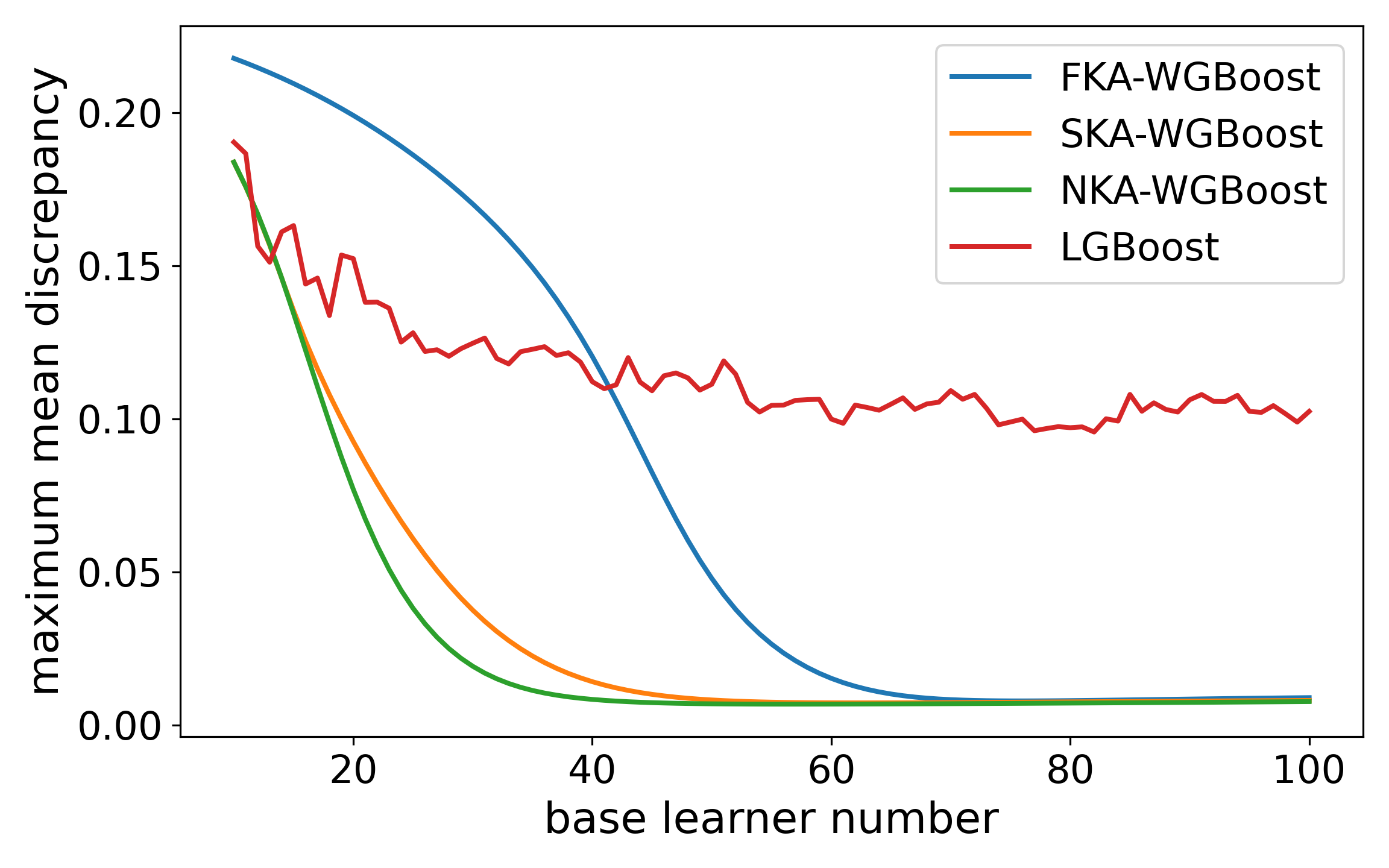
Figure 3: Approximation error and computational time of the four algorithms. Left panel: approximation error of each algorithm measured by the MMD average over the inputs. Right panel: computational time with respect to the base learner number in common logarithm scale.

Figure 3 demonstrates that SKA-WGBoost and NKA-WGBoost reduce the approximation error most efficiently, while NKA-WGBoost takes the longest computational time among others. As in Algorithm 4, the computation of the full approximate Wasserstein Newton direction requires the inverse and product of the $(N\times d)\times(N\times d)$ block matrices for the particle number $N$ and the particle dimension $d$. The computation of the diagonal approximate Wasserstein Newton direction requires only elementwise division of the $d$-dimensional vectors. The error decay of LGBoost is not as fast as the other WGBoost algorithms and shows stochasticity due to the Gaussian noise used in the algorithm. We therefore recommend to use SKA-WGBoost for better performance and efficient computation. Figure 4 depicts the output of each algorithm with 100 base learners trained.

(a) FKA-WGBoost

(b) SKA-WGBoost

(c) NKA-WGBoost

(d) LGBoost

Figure 4: Illustration of the output of the four algorithms (red line) with 100 base learners trained. The blue area corresponds to the 95% high probability region of the target distribution.

Appendix F Additional Detail of Application

This section describes additional details of the applications in Section 4. All the experiments were performed with x86-64 CPUs, where some of them were parallelised up to 10 CPUs and the rest uses 1 CPU. The scripts to reproduce all the experiments are provided in the source code. Sections F.1, F.2 and F.3 describe additional details of the applications in, respectively, Sections 4.1, 4.2 and 4.3. Section F.4 describes a choice of initial constants $\{\vartheta_{0}^{n}\}_{n=1}^{N}$ for the WGBoost algorithm used in Section 4.

F.1 Detail of Section 4.1

Figure 3 shows the output of the WGBoost algorithm for the old faithful geyser data. The normal output distribution $\mathcal{N}(y\mid m,\sigma)$ in Example 1 was used in Section 4.1. As mentioned in Section 3.1, we reparametrise a parameter that lies in a subset of the Euclidean space as one in the Euclidean space, which is the standard practice in Bayesian computation [20]. The normal output distribution $\mathcal{N}(y\mid m,\sigma)$ has the scale parameter $\sigma$ that lies only in the positive domain of the Euclidean space $\mathbb{R}$. We reparametrised the scale parameter by the log transform $\sigma^{\prime}:=\log(\sigma)$. The inverse of the log transform is the exponential transform $\sigma=\exp(\sigma^{\prime})$. It follows from change of variable that the posterior on $(m,\sigma^{\prime})$ built on a datum $y_{i}$ and the prior in Example 1 is given by

$$\pi_{i}(m,\sigma^{\prime})\propto\exp\left(-\frac{1}{2}\frac{(y_{i}-m)^{2}}{\exp(\sigma^{\prime})^{2}}\right)\times\exp\left(-\frac{1}{2}\frac{m^{2}}{10^{2}}\right)\times\frac{1}{\exp(\sigma^{\prime})^{1.01}}\exp\left(-\frac{0.01}{\exp(\sigma^{\prime})}\right)$$ (82)

up to the normalising constant, where we used the Jacobian determinant $|d\sigma/d\sigma^{\prime}|=\exp(\sigma^{\prime})$.

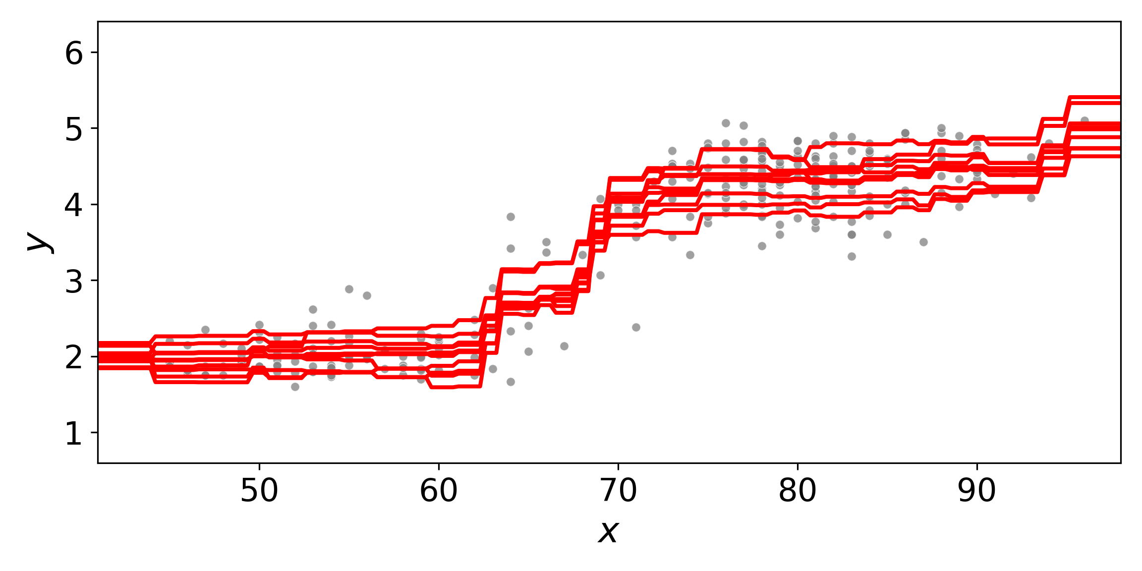
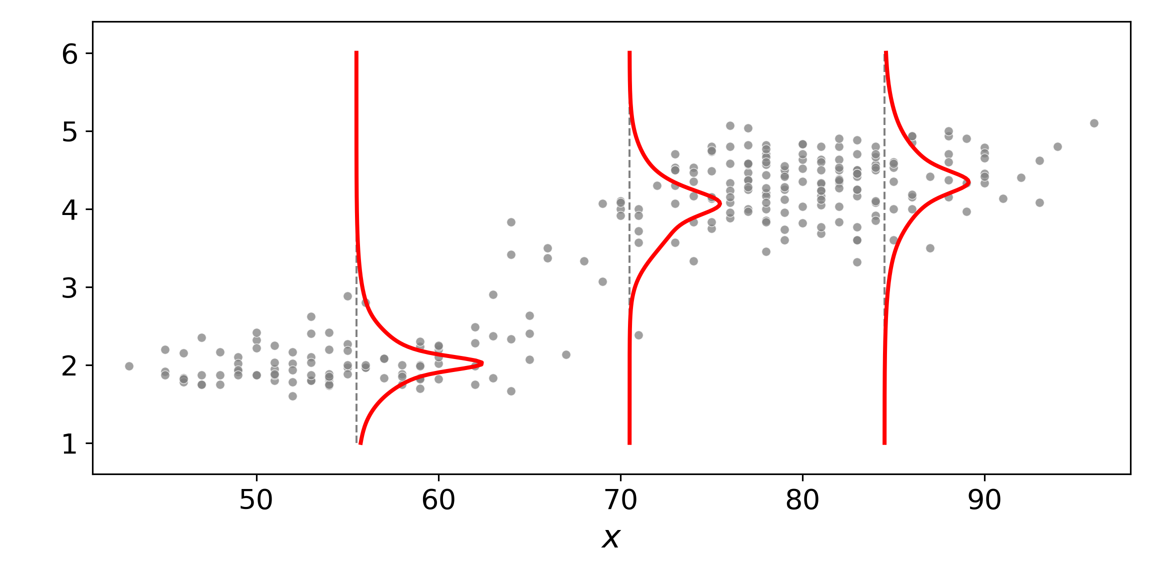
Figure 5: Conditional density estimation by the WGBoost algorithm for the old faithful geyser dataset. Left panel: distributional estimate (10 particles) of the location parameter $m$ for each input. Right panel: estimated density by the predictive distribution (10) based on the output particles.

F.2 Detail of Section 4.2

The same reparametrisation of the normal output distribution as Section F.2 was used in Section 4.2. For test data $\{x_{i},y_{i}\}_{i=1}^{D}$, the NLL and RMSE of each algorithm were computed by

$$\text{NLL}=-\frac{1}{D}\sum_{i=1}^{D}\log p(y_{i}\mid x_{i})\quad\text{and}\quad\text{RMSE}=\sqrt{\frac{1}{D}\sum_{i=1}^{D}(y_{i}-\hat{y}_{i})^{2}}$$ (83)

based on the provided predictive distribution $p(y_{i}\mid x_{i})$ and the point prediction $\hat{y}_{i}$. For the WGBoost algorithm, the training outputs were standardised. Accordingly, the test outputs were standardised as $y_{i}^{\prime}=(y_{i}-y_{\text{mean}}^{\text{train}})/y_{\text{std}}^{\text{train}}$ with the mean $y_{\text{mean}}^{\text{train}}$ and standard deviation $y_{\text{std}}^{\text{train}}$ of the training outputs. The WGBoost algorithm provides the predictive distribution $p(y_{i}^{\prime}\mid x_{i})$ and point prediction $\hat{y}_{i}^{\prime}$ for the standardised outputs $y_{i}^{\prime}$. The NLL and RMSE for the original outputs $y_{i}$ can be computed as follows:

NLL $$=-\frac{1}{D}\sum_{i=1}^{D}\log p(y_{i}\mid x_{i})=-\frac{1}{D}\sum_{i=1}^{D}\log p(y_{i}^{\prime}\mid x_{i})+\log y_{\text{std}}^{\text{train}},$$ (84)

RMSE $$=\sqrt{\frac{1}{D}\sum_{i=1}^{D}(y_{i}-(y_{\text{mean}}^{\text{train}}+y_{\text{std}}^{\text{train}}\times\hat{y}_{i}^{\prime}))^{2}}=y_{\text{std}}^{\text{train}}\sqrt{\frac{1}{D}\sum_{i=1}^{D}(y_{i}^{\prime}-\hat{y}_{i}^{\prime})^{2}}$$ (85)

where the equality of the NLL follows from change of variable $p(y_{i}\mid x_{i})=p(y_{i}^{\prime}\mid x_{i})/y_{\text{std}}^{\text{train}}$ and the equality of the RMSE follows from rearranging the terms.

We provide a brief description of each algorithm used for the comparison. For each algorithm, the normal location-scale output distribution $p(y\mid m,\sigma)$ was specified on the output space $\mathcal{Y}$ and the algorithm produces an estimate of $(m,\sigma)$ at each input $x$.

• MCDropout [9] trains a single neural network $F$ while dropping out each parameter with some Bernoulli probability. It can be interpreted as a variational approximation of a Bayesian neural network. It generates multiple subnetworks $\{F^{n}\}_{n=1}^{N}$ by subsampling the network parameter by the dropout. The predictive distribution $p(y\mid x)$ is given by the model averaging $(1/N)\sum_{i=1}^{N}p(y\mid(m,\sigma)=F^{n}(x))$ for each input $x$.

• DEnsemble [10] simply trains independent copies $\{F^{n}\}_{n=1}^{N}$ of a neural network $F$ in parallel. It is one of the mainstream approaches to uncertainty quantification based on deep learning. The predictive distribution is given by the model averaging as in MCDropout.

• CDropout [55] consider a continuous relaxation of the Bernoulli random variable used in MCDropout to optimise the Bernoulli probability of the dropout. It generates multiple subnetworks $\{F^{n}\}_{n=1}^{N}$ by subsampling the network parameter by the dropout with the optimised probability. The predictive distribution is same as MCDropout.

• NGBoosting [33] is a family of gradient booting that use the natural gradient [67] of the output distribution as a target response of each base learner. In contrast to other methods, NGBoost outputs a single value $F(x)$ to be plugged into the output-distribution parameter $\theta$. The predictive distribution $p(y\mid x)$ is given by $p(y\mid(m,\sigma)=F(x))$ for each input $x$.

• DEvidential [13] extends deep evidential learning [11], originally proposed in classification settings, to regression settings. It considers the case where the posterior of the output distribution falls into a conjugate parametric form, and approximates the parameter by a neural network. The predictive distribution is also given in a conjugate closed-form.

F.3 Detail of Section 4.3

Similarly to the normal output distribution used in Sections 4.1 and 4.2, we reparametrised the categorical output distribution used in Section 4.3. The categorical output distribution $\mathcal{C}(y\mid q)$ in Example 2 has a class probability parameter $q=[q_{1},\dots,q_{k}]$ in the simplex $\Delta_{k}$. We reparametrised the parameter $q$ by the log-ratio transform $q^{\prime}:=[\log(q_{1}/q_{k}),\dots,\log(q_{k-1}/q_{k})]\in\mathbb{R}^{k-1}$ that maps from the simplex $\Delta_{k}$ to the Euclidean space $\mathbb{R}^{k-1}$ [45]. The inverse is the logistic transform

$$q=\left[\frac{\exp(q^{\prime}_{1})}{z_{k}},\dots,\frac{\exp(q^{\prime}_{k-1})}{z_{k}},\frac{1}{z_{k}}\right]\in\Delta_{k}\quad\text{where}\quad z_{k}=1+\sum_{j=1}^{k-1}\exp(q^{\prime}_{j}).$$ (86)

The logistic normal distribution on $q$ corresponds to a normal distribution on $q^{\prime}$ by change of variable [45]. By change of variable, the posterior on $q^{\prime}$ with a datum $y_{i}$ and the prior in Example 2 is

$$\pi_{i}(q^{\prime})\propto\prod_{j=1}^{k-1}\left(\frac{\exp(q^{\prime}_{j})}{z_{k}}\right)^{[y_{i}=j]}\times\exp\left(-\frac{1}{2}\frac{\|q^{\prime}\|^{2}}{10^{2}}\right)$$ (87)

up to the normalising constant, where $[y_{i}=j]$ is $1$ if $y_{i}$ is the $j$-th class label and $0$ otherwise.

We provide a brief description of each algorithm used in comparison with WGBoost. MCDropout and DEnsemble are described in Section F.2.

• DDistillation [58] learns the parameter of a Dirichlet distribution over the simplex $\Delta_{k}$ by a neural network using the output of DEnsemble. The output of multiple networks in DEnsemble is distilled into the a Dirichlet distribution controlled by one single network.

• PNetwork [14] considers the case where the posterior of the categorical output distribution falls into a Dirichlet distribution similarly to deep evidential learning [11]. It learns the parameter of the posterior given in the form of the Dirichlet distribution by a neural network.

F.4 Choice of Initial State of WGBoost

In standard gradient boosting, the initial state of gradient boosting is specified by a constant that most fits given data. Similarly, for the applications in Section 4, we specified the initial state $\{\vartheta_{0}^{n}\}_{n=1}^{N}$ of the WGBoost algorithm by a set of constants that most fits the given target distributions in average. We find such a set of constants by performing an approximate Wasserstein gradient flow averaged over all the target distributions. Specifically, given the term $\mathcal{G}_{i}(\mu)$ in Algorithm 1, we define $\bar{\mathcal{G}}(\mu):=(1/D)\sum_{i=1}^{D}\mathcal{G}_{i}(\mu)$ and perform the update scheme of a set of $N$ particles $\{\bar{\vartheta}_{m}^{n}\}_{n=1}^{N}$:

$$\begin{bmatrix}\bar{\vartheta}_{m+1}^{1}\\ \vdots\\ \bar{\vartheta}_{m+1}^{N}\end{bmatrix}=\begin{bmatrix}\bar{\vartheta}_{m}^{1}\\ \vdots\\ \bar{\vartheta}_{m}^{N}\end{bmatrix}+\nu_{0}\begin{bmatrix}-[\bar{\mathcal{G}}(\hat{\pi}_{m})](\bar{\vartheta}_{m}^{1})\\ \vdots\\ -[\bar{\mathcal{G}}(\hat{\pi}_{m})](\bar{\vartheta}_{m}^{N})\end{bmatrix}$$ (88)

with the learning rate $\nu_{0}=0.01$ and the maximum step number $M_{0}=5000$. The initial particle locations for this update scheme were sampled from a standard normal distribution. We specified the initial state $\{\vartheta_{0}^{n}\}_{n=1}^{N}$ by the set of particles $\{\bar{\vartheta}_{M_{0}}^{n}\}_{n=1}^{N}$ obtained though this scheme.

References

- [1] Ravid Shwartz-Ziv and Amitai Armon. Tabular data: Deep learning is not all you need. Information Fusion, 81:84–90, 2022.
- [2] Moloud Abdar, Farhad Pourpanah, Sadiq Hussain, Dana Rezazadegan, Li Liu, Mohammad Ghavamzadeh, Paul Fieguth, Xiaochun Cao, Abbas Khosravi, U. Rajendra Acharya, Vladimir Makarenkov, and Saeid Nahavandi. A review of uncertainty quantification in deep learning: Techniques, applications and challenges. Information Fusion, 76:243–297, 2021.
- [3] Eric Topol. High-performance medicine: the convergence of human and artificial intelligence. Nature Medicine, 25:44–56, 2019.
- [4] Sorin Grigorescu, Bogdan Trasnea, Tiberiu Cocias, and Gigel Macesanu. A survey of deep learning techniques for autonomous driving. Journal of Field Robotics, 37(3):362–386, 2020.
- [5] Matthew Richardson, Ewa Dominowska, and Robert Ragno. Predicting clicks: estimating the click-through rate for new ads. In Proceedings of the 16th International Conference on World Wide Web, page 521–530, 2007.
- [6] Christopher Burges. From ranknet to lambdarank to lambdamart: An overview. Learning, 11, 2010.
- [7] Byron P. Roe, Hai-Jun Yang, Ji Zhu, Yong Liu, Ion Stancu, and Gordon McGregor. Boosted decision trees as an alternative to artificial neural networks for particle identification. Nuclear Instruments and Methods in Physics Research Section A: Accelerators, Spectrometers, Detectors and Associated Equipment, 543(2):577–584, 2005.
- [8] James Bennett and Stan Lanning. The Netflix prize. In Proceedings of the KDD Cup Workshop 2007, pages 3–6, 2007.
- [9] Yarin Gal and Zoubin Ghahramani. Dropout as a Bayesian approximation: Representing model uncertainty in deep learning. In Proceedings of The 33rd International Conference on Machine Learning, volume 48 of Proceedings of Machine Learning Research, pages 1050–1059. PMLR, 2016.
- [10] Balaji Lakshminarayanan, Alexander Pritzel, and Charles Blundell. Simple and scalable predictive uncertainty estimation using deep ensembles. In Advances in Neural Information Processing Systems, volume 30, 2017.
- [11] Murat Sensoy, Lance Kaplan, and Melih Kandemir. Evidential deep learning to quantify classification uncertainty. In Advances in Neural Information Processing Systems, volume 31, 2018.
- [12] Jakob Gawlikowski, Cedrique Rovile Njieutcheu Tassi, Mohsin Ali, Jongseok Lee, Matthias Humt, Jianxiang Feng, Anna Kruspe, Rudolph Triebel, Peter Jung, Ribana Roscher, Muhammad Shahzad, Wen Yang, Richard Bamler, and Xiao Xiang Zhu. A survey of uncertainty in deep neural networks. Artificial Intelligence Review, 56:1513–1589, 2023.
- [13] Alexander Amini, Wilko Schwarting, Ava Soleimany, and Daniela Rus. Deep evidential regression. In Advances in Neural Information Processing Systems, volume 33, pages 14927–14937, 2020.
- [14] Bertrand Charpentier, Daniel Zügner, and Stephan Günnemann. Posterior network: Uncertainty estimation without OOD samples via density-based pseudo-counts. In Advances in Neural Information Processing Systems, volume 33, pages 1356–1367. Curran Associates, Inc., 2020.
- [15] Dennis Thomas Ulmer, Christian Hardmeier, and Jes Frellsen. Prior and posterior networks: A survey on evidential deep learning methods for uncertainty estimation. Transactions on Machine Learning Research, 2023.
- [16] Edouard Capellier, Franck Davoine, Veronique Cherfaoui, and You Li. Evidential deep learning for arbitrary lidar object classification in the context of autonomous driving. In 2019 IEEE Intelligent Vehicles Symposium (IV), pages 1304–1311, 2019.
- [17] Patrick Hemmer, Niklas Kühl, and Jakob Schöffer. Deal: Deep evidential active learning for image classification. In 2020 19th IEEE International Conference on Machine Learning and Applications (ICMLA), pages 865–870, 2020.
- [18] Ava P. Soleimany, Alexander Amini, Samuel Goldman, Daniela Rus, Sangeeta N. Bhatia, and Connor W. Coley. Evidential deep learning for guided molecular property prediction and discovery. ACS Central Science, 7(8):1356–1367, 2021.
- [19] Jakob Gawlikowski, Sudipan Saha, Anna Kruspe, and Xiao Xiang Zhu. An advanced Dirichlet prior network for out-of-distribution detection in remote sensing. IEEE Transactions on Geoscience and Remote Sensing, 60:1–19, 2022.
- [20] Andrew Gelman, John B. Carlin, Hal S. Stern, David B. Dunson, Aki Vehtari, and Donald B. Rubin. Bayesian Data Analysis. Chapman and Hall/CRC, 3rd ed. edition, 2013.
- [21] Trevor Hastie, Robert Tibshirani, and Jerome Friedman. The Elements of Statistical Learning. Springer New York, 2009.
- [22] Tianqi Chen and Carlos Guestrin. XGBoost: A scalable tree boosting system. In Proceedings of the 22nd ACM SIGKDD International Conference on Knowledge Discovery and Data Mining, KDD ’16, page 785–794, 2016.
- [23] Guolin Ke, Qi Meng, Thomas Finley, Taifeng Wang, Wei Chen, Weidong Ma, Qiwei Ye, and Tie-Yan Liu. LightGBM: A highly efficient gradient boosting decision tree. In Advances in Neural Information Processing Systems, volume 30, 2017.
- [24] C’edric Villani. Topics in Optimal Transportation. Americal Mathematical Society, 2003.
- [25] Luigi Ambrosio, Nicola Gigli, and Giuseppe Savaré. Gradient Flows In Metric Spaces and in the Space of Probability Measures. Birkhäuser Basel, 2005.
- [26] Filippo Santambrogio. {Euclidean, metric, and Wasserstein} gradient flows: an overview. Bulletin of Mathematical Sciences, 7:87–154, 2017.
- [27] Qiang Liu. Stein variational gradient descent as gradient flow. In Advances in Neural Information Processing Systems, volume 30, 2017.
- [28] Jos’e Antonio Carrillo, Katy Craig, and Francesco S. Patacchini. A blob method for diffusion. Calculus of Variations and Partial Differential Equations, 58(53), 2019.
- [29] Yifei Wang, Peng Chen, and Wuchen Li. Projected Wasserstein gradient descent for high-dimensional Bayesian inference. SIAM/ASA Journal on Uncertainty Quantification, 10(4):1513–1532, 2022.
- [30] Dimitra Maoutsa, Sebastian Reich, and Manfred Opper. Interacting particle solutions of Fokker-Planck equations through gradient-log-density estimation. Entropy (Basel), 22(8):802, 2020.
- [31] Ye He, Krishnakumar Balasubramanian, Bharath K. Sriperumbudur, and Jianfeng Lu. Regularized Stein variational gradient flow. arXiv:2211.07861, 2022.
- [32] Jerome H. Friedman. Greedy function approximation: A gradient boosting machine. The Annals of Statistics, 29(5):1189–1232, 2001.
- [33] Tony Duan, Avati Anand, Daisy Yi Ding, Khanh K. Thai, Sanjay Basu, Andrew Ng, and Alejandro Schuler. NGBoost: Natural gradient boosting for probabilistic prediction. In Proceedings of the 37th International Conference on Machine Learning, volume 119 of Proceedings of Machine Learning Research, pages 2690–2700. PMLR, 2020.
- [34] Llew Mason, Jonathan Baxter, Peter Bartlett, and Marcus Frean. Boosting algorithms as gradient descent. In Advances in Neural Information Processing Systems, volume 12, 1999.
- [35] Peter Bühlmann and Torsten Hothorn. Boosting Algorithms: Regularization, Prediction and Model Fitting. Statistical Science, 22(4):477 – 505, 2007.
- [36] Leo Grinsztajn, Edouard Oyallon, and Gael Varoquaux. Why do tree-based models still outperform deep learning on typical tabular data? In Advances in Neural Information Processing Systems, volume 35, pages 507–520, 2022.
- [37] Piotr Florek and Adam Zagdański. Benchmarking state-of-the-art gradient boosting algorithms for classification. arXiv:2305.17094, 2023.
- [38] Zhendong Zhang and Cheolkon Jung. GBDT-MO: Gradient-boosted decision trees for multiple outputs. IEEE Transactions on Neural Networks and Learning Systems, 32(7):3156–3167, 2021.
- [39] Tianqi Chen, Sameer Singh, Ben Taskar, and Carlos Guestrin. Efficient Second-Order Gradient Boosting for Conditional Random Fields. In Proceedings of the Eighteenth International Conference on Artificial Intelligence and Statistics, volume 38 of Proceedings of Machine Learning Research, pages 147–155. PMLR, 2015.
- [40] Leo Breiman, Jerome Friedman, R.A. Olshen, and Charles J. Stone. Classification and Regression Trees. Chapman and Hall/CRC, 1984.
- [41] Jerome H. Friedman. Stochastic gradient boosting. Computational Statistics & Data Analysis, 38(4):367–378, 2002.
- [42] Gianluca Detommaso, Tiangang Cui, Youssef Marzouk, Alessio Spantini, and Robert Scheichl. A Stein variational Newton method. In Advances in Neural Information Processing Systems, volume 31, 2018.
- [43] Yifei Wang and Wuchen Li. Information Newton’s flow: second-order optimization method in probability space. arXiv:2001.04341, 2020.
- [44] Malay Ghosh. Objective priors: An introduction for frequentists. Statistical Science, 26(2):187–202, 2011.
- [45] J. Aitchison and S. M. Shen. Logistic-normal distributions: Some properties and uses. Biometrika, 67(2):261–272, 1980.
- [46] Qiang Liu and Dilin Wang. Stein variational gradient descent: A general purpose Bayesian inference algorithm. In Advances in Neural Information Processing Systems, volume 29, 2016.
- [47] Dilin Wang, Zhe Zeng, and Qiang Liu. Stein variational message passing for continuous graphical models. In Proceedings of the 35th International Conference on Machine Learning, volume 80 of Proceedings of Machine Learning Research, pages 5219–5227. PMLR, 2018.
- [48] Alexander Lambert, Fabio Ramos, Byron Boots, Dieter Fox, and Adam Fishman. Stein variational model predictive control. In Proceedings of the 2020 Conference on Robot Learning, volume 155 of Proceedings of Machine Learning Research, pages 1278–1297. PMLR, 2021.
- [49] Anna Korba, Adil Salim, Michael Arbel, Giulia Luise, and Arthur Gretton. A non-asymptotic analysis for Stein variational gradient descent. In Advances in Neural Information Processing Systems, volume 33, pages 4672–4682, 2020.
- [50] Sinho Chewi, Thibaut Le Gouic, Chen Lu, Tyler Maunu, and Philippe Rigollet. SVGD as a kernelized Wasserstein gradient flow of the chi-squared divergence. In Advances in Neural Information Processing Systems, volume 33, pages 2098–2109, 2020.
- [51] Andre Wibisono. Sampling as optimization in the space of measures: The Langevin dynamics as a composite optimization problem. In Proceedings of the 31st Conference On Learning Theory, volume 75 of Proceedings of Machine Learning Research, pages 2093–3027. PMLR, 2018.
- [52] Gareth O. Roberts and Richard L. Tweedie. Exponential convergence of Langevin distributions and their discrete approximations. Bernoulli, 2(4):341 – 363, 1996.
- [53] Jose Miguel Hernandez-Lobato and Ryan Adams. Probabilistic backpropagation for scalable learning of Bayesian neural networks. In Proceedings of the 32nd International Conference on Machine Learning, volume 37 of Proceedings of Machine Learning Research, pages 1861–1869. PMLR, 2015.
- [54] Sanford Weisberg. Applied Linear Regression. John Wiley & Sons, 1985.
- [55] Yarin Gal, Jiri Hron, and Alex Kendall. Concrete dropout. In Advances in Neural Information Processing Systems, volume 30, 2017.
- [56] Dheeru Dua and Casey Graff. UCI machine learning repository, 2017.
- [57] Jingkang Yang, Kaiyang Zhou, Yixuan Li, and Ziwei Liu. Generalized out-of-distribution detection: A survey. arXiv:2110.11334, 2024.
- [58] Andrey Malinin, Bruno Mlodozeniec, and Mark Gales. Ensemble distribution distillation. In International Conference on Learning Representations, 2020.
- [59] Filippo Santambrogio. Optimal Transport for Applied Mathematicians. Birkhäuser Cham, 2015.
- [60] Mingxuan Yi and Song Liu. Bridging the gap between variational inference and Wasserstein gradient flows, 2023.
- [61] Michael Arbel, Anna Korba, Adil Salim, and Arthur Gretton. Maximum mean discrepancy gradient flow. In Advances in Neural Information Processing Systems, volume 32, 2019.
- [62] Richard Jordan, David Kinderlehrer, and Felix Otto. The variational formulation of the Fokker–Planck equation. SIAM Journal on Mathematical Analysis, 29(1):1–17, 1998.
- [63] Grigorios A. Pavliotis. Stochastic Processes and Applications. Springer New York, 2014.
- [64] Vern I. Paulsen and Mrinal Raghupathi. An Introduction to the Theory of Reproducing Kernel Hilbert Spaces. Cambridge University Press, 2016.
- [65] Alex Leviyev, Joshua Chen, Yifei Wang, Omar Ghattas, and Aaron Zimmerman. A stochastic Stein variational Newton method. arXiv:2204.09039, 2022.
- [66] Alex Smola, Arthur Gretton, Le Song, and Bernhard Schölkopf. A Hilbert space embedding for distributions.
- [67] Shun ichi Amari. Information Geometry and Its Applications. Springer Tokyo, 2016.