Joint Physics Analysis Center
Nonperturbative aspects of the electromagnetic pion form factor at high energies
Abstract
The structure of hadronic form factors at high energies and their deviations from perturbative quantum chromodynamics provide insight on nonperturbative dynamics. Using an approach that is consistent with dispersion relations, we construct a model that simultaneously accounts for the pion wave function, gluonic exchanges, and quark Reggeization. In particular, we find that quark Reggeization can be investigated at high energies by studying scaling violation of the form factor.
I Introduction
Form factors encode information about hadron composition. For example, form factors at low energies have been used to discriminate between constituent quark and mesonic degrees of freedom Perdrisat et al. (2007); Roberts et al. (2021); Barabanov et al. (2021), while at large momentum transfer they can be used to investigate the short distance interactions between partons inside a hadron. The pion electromagnetic form factor plays a special role because of the simplicity of the theoretical prediction Li and Sterman (1992); O’Connell et al. (1997); Stefanis et al. (1999); Bakulev et al. (2004); Gorchtein et al. (2012); Perry et al. (2019). At high energies, partons are asymptotically free. Therefore, when the photon interacts with one of the partons of a hadron, it is possible for the large momentum transfer to be shared internally between a few constituents via hard QCD interactions in such a way that the soft wave functions are shielded from large momentum flows Brodsky and Farrar (1973); Duncan and Mueller (1980); Efremov and Radyushkin (1980a); Lepage and Brodsky (1980). Hence, the contributions from hard and soft processes factorize, and as one can rely on perturbative QCD (pQCD) to calculate the spacelike charged pion electromagnetic form factor Farrar and Jackson (1979); Efremov and Radyushkin (1980b); Lepage and Brodsky (1979)
| (1) |
Here is the pion decay constant capturing the contribution from the soft processes, is the running QCD coupling, and is the photon virtuality. The perturbative result in the spacelike region can be analytically continued to the timelike region , where is the energy squared of the final system. Several measurements of the pion and other pseudo-scalar meson form factors have been performed in the past Brown et al. (1973); Bebek et al. (1976); Volmer et al. (2001); Aul’chenko et al. (2006); Aloisio et al. (2005); Aul’chenko et al. (2006); Achasov et al. (2006); Horn et al. (2006); Tadevosyan et al. (2007); Horn et al. (2008); Akhmetshin et al. (2007); Aubert et al. (2009); Lees et al. (2012); Ablikim et al. (2016); Ambrosino et al. (2011); Seth et al. (2013), with more experiments scheduled for the future Abdul Khalek et al. (2022); Accardi et al. (2023). It was argued in Refs. Isgur and Llewellyn Smith (1984, 1989); Belyaev and Radyushkin (1996) that for the soft contributions dominate, so the asymptotic behavior of Eq. 1 may have not yet been reached Gousset and Pire (1995). Indeed, the analysis of Seth et al. (2013) from CLEO-c finds two data points at and that are approximately a factor of two above the pQCD prediction. In light of this discrepancy between the pQCD prediction and experimental data at currently accessible energies, it is interesting to study models that transition between soft and hard processes, which may also be more applicable to energy regions relevant to current experiments. We use the framework of dispersion relations to ensure that the fundamental -matrix constraints are satisfied while we model microscopic effects relevant to the asymptotic behavior of the pion form factor. For simplicity, we treat all particles as scalars in an attempt to demonstrate how different microscopic models yield varying asymptotic energy dependencies. Our calculations should not be interpreted as predictions for the high energy behavior of the pion form factor, but rather as an exploration of the types of energy asymptotics which one might observe for physical quarks.
The rest of the paper is organized as follows. In Section II the models are presented and discussed individually and in Section III they are compared and the conclusions summarized.
II Models
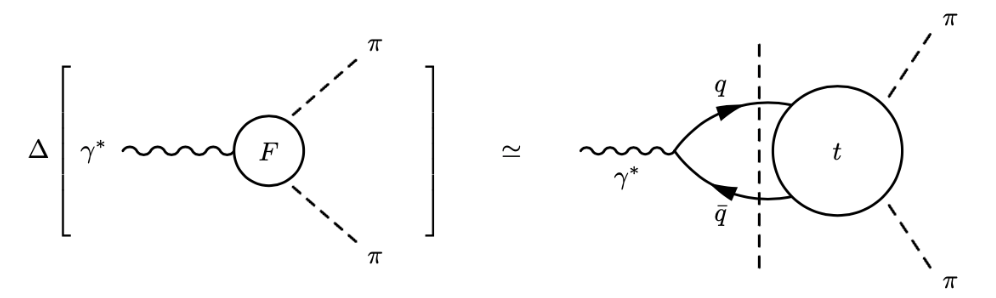
The electromagnetic pion form factor can be written in terms of its discontinuity across the unitary cut Gorchtein et al. (2012), using a dispersion relation
| (2) |
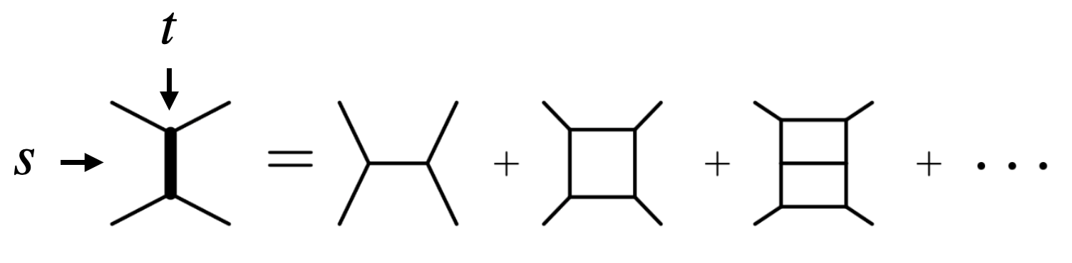
In the high energy regime, as illustrated in Fig. 1, it can be approximated by
| (3) |
where is the threshold, and and are transition amplitudes from a virtual photon to a (on-shell) pair, and from the pair to two pions, respectively. We note that the actual value of is irrelevant, given that we are interested in the high energy behavior. We use the notation to represent the phase space factor for the production of the on-shell quark-antiquark pair. The dispersive representation relies entirely on physical on-shell quantities, which allows for a straightforward physics interpretation. We are interested in understanding the role of various mechanisms contributing to at high energies.
Asymptotically the two-body phase space , thus at some large the discontinuity originates from a intermediate state and . At large , the photon decays to a quark and an antiquark, which, in the rest frame of the virtual photon, move in opposite directions with large momenta . Hadronization dynamics is contained in the (on-shell) amplitude . Both the quark and the antiquark must pull a comoving antiquark or quark respectively from the vacuum to form the two outgoing pions. This can be achieved only if one of the initial two quarks radiates a hard gluon which may then decay to produce the . In principle, the decay of the hard gluon can be a multi-step process that fills in the rapidity gap between the initial quarks from the photon decay. This multiparticle production corresponds to ladder exchanges, leading to an effective amplitude, Fig. 2, with a Reggeized quark exchanged in the channel Fadin and Sherman (1977); Strikman (2008); Gorchtein et al. (2012).
To obtain the behavior, the denominator of LABEL:{eq:dicFormFactorGeneral} can be expanded, resulting in a sum of moments of the discontinuity of the form factor
| (4) |
The convergence of Eq. 2 implies that the integral over becomes negligible as , and we can keep only the sum of moments of the first term. Hence, if we were interested in an amplitude that behaves according to at large , we should require that the first moments of the discontinuity of the form factor vanish, i.e.
| (5) |
where . Therefore, a positive leads to a falloff (modulo logarithms) of the form factor. A falloff faster than implies the existence of intermediate states other than which contribute destructively to the discontinuity of . This is analogous to the cancellation found in Regge cut models Amati et al. (1962).
In what follows, we discuss the role of the individual mechanisms that contribute to the form factor and their impact in the asymptotic behavior.
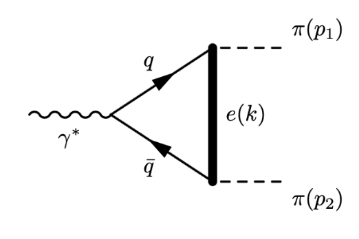
II.1 Pointlike model
To establish a point of reference for the comparison of different microscopic contributions, we first consider a model, as depicted in Fig. 2, where the interaction is pointlike, the exchanged particle is not Reggeized, and there are no soft pion wave functions. This makes all the interactions as hard as possible. The model gives an upper limit for the behavior of the physical form factor at high energies. In Fig. 2 the propagators are and the transition amplitude is mediated by a (scalar) quark exchange. Hence, disregarding the normalization, we can write the pointlike form factor as
| (6) |
where and , is the quark mass, and is the exchanged particle mass. Its dispersive representation reads
| (7) |
where the discontinuity is computed from the diagram in Fig. 2 by putting the pair on shell according to the Cutkosky’s cutting rules Collins (2009); Eden et al. (1966). This corresponds to the S wave of the -channel partial wave projection of the scattering amplitude
| (8) |
where
| (9) |
with and , the -channel scattering angle between one of the quarks and the pion it hadronizes into. The phase space reads . After integrating over the scattering angle one finds for the discontinuity ,
| (10) |
We can now examine what Eq. 9 implies for the large behavior of Eq. 7. For , the quark exchange behaves as and , so the integration over produces a contribution and the integration provides a second , leading to
| (11) |
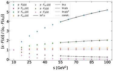
In Fig. 3 we show the numerical evaluation of using GeV and GeV compared to the asymptotic behavior in Eq. 11. The agreement is apparent.
II.2 Pion wave function effects
The presented pointlike model lacks nonperturbative effects from the pion wave function. In the constituent quark model the pion can be described as a state. Therefore we can introduce a pion wave function by replacing the point-like quark propagators with constituent quark propagators. This is achieved by employing a dressed quark propagator which for simplicity, takes the form
| (12) |
where the subscript indicates the softening power. We have several softening options depending on how many and which propagators are softened. First we soften the two horizontal propagators (see Fig. 2). The form factor reads
| (13) |
Obviously, if , the hard production result is recovered. This simple model satisfies the condition of Eq. 5 providing a form factor whose leading high energy behavior depends on according to
| (14) |
as shown in Fig. 3 where the result of integrating Eq. 13 using Feynman parameters (see Section A.1) is compared to the asymptotic prediction of Eq. 14. Therefore, this substitution with an arbitrary integer power cancels the first moments of the discontinuity of the form factor, yielding a softer pion form factor.
We can modify only the exchanged quark propagator in Fig. 2 following Eq. 12
| (15) |
which at high energy behaves as (see Section A.2)
| (16) |
This is confirmed in Fig. 3 where the numerical integration of Eq. 15, using the same masses as in Section II.1, yields a result whose asymptotic behavior is independent of that matches the Eq. 16 expectation. Hence, the asymptotic falloff of the form factor is not sensitive to the softening of the exchanged quark. This is expected, because the momentum flowing through the vertical propagator in Fig. 2 can always be kept finite by having the quarks hadronize to pions with little transverse momentum, so that the hard momentum never flows through the exchanged quark line.
Finally, if we soften only one of the quark propagators connected to the photon vertex and the exchanged quark, we obtain
| (17) |
We find that the high energy behavior does not depend on (see Section A.3)
| (18) |
This result is a consequence of the large momentum flowing through the perturbative propagator which leads to a nonvanishing 0 moment in Eq. 5. Therefore, the first term in the Eq. 4 expansion contributes, leading to a asymptotic behavior. In Fig. 3, the numerical integration of Eq. 17, using the same masses as in Section II.1, is compared to the asymptotic Eq. 18.
These results show why the notion of a pion wave function should not be associated exclusively with the quark-pion vertex function, which is a function of only, but with the intermediate state in the pion channels. These intermediate states contain the exchanged quark and one of the quark lines connected to the photon. Therefore a physical model with soft pion wave functions, in a dispersive representation, can be realized through modification of the quark propagators. Such propagators emerge for example from calculations based on the QCD Dyson-Schwinger equations Roberts (2015).
Given that pions are soft, to bring the power behaviour of the form factor back to as shown above, it is sufficient to screen only one of the two wave functions. This is the role of the one gluon exchange, which effectively short-circuits one of the pion wave functions.
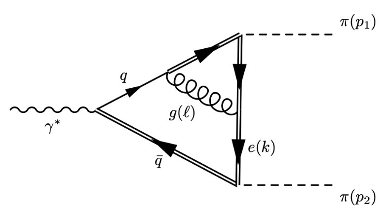
II.3 One gluon exchange
As the energy of the photon increases, the spatial resolution of the photon becomes fine enough that the individual gluon exchange at the pion vertex becomes relevant. Therefore, the gluon exchange in Fig. 4 contributes to the high energy behavior of the form factor. If we combine this gluon exchange and the soft quark propagators that account for the pion wave function in Eq. 13, we obtain
| (19) |
where
| (20) |
is the integral over the softened quark-gluon-quark triangle. Numerical and analytical (see Appendix B) results for Eq. 19 show that regardless of for the limit. The results show that the introduction of the gluon loop effectively screens the form factor from the softening effects of the nonperturbative power law modification leading to a
| (21) |
behavior.
II.4 Reggeized model
At high energies, the contribution of the -channel exchange to the process is expected to be dominated not by a single quark exchange but by the corresponding Regge trajectory Fadin and Sherman (1977); Strikman (2008). This effectively describes multiparticle production at high energies and introduces energy dependence to which otherwise would be only a function of the momentum transferred between the quark and the pion as in Eq. 6. Hence, once the angular dependence is integrated, the asymptotic behavior of the amplitude in Fig. 2 is dominated by the leading Regge trajectory of the exchanged particle as follows
| (22) |
As discussed in LABEL:{sec:pert}, asymptotically, the form factor is dominated by the region. Therefore, the finite dependence of the Regge residues does not affect the asymptotic behavior and can be safely ignored. Once the Regge trajectory is determined, the pion form factor can be calculated by replacing the exchanged quark propagator in Eq. 6 by
| (23) |
leading to
| (24) |
The form factor is straightforwardly calculated using the dispersive integral of Eq. 2 with the discontinuity given by
| (25) |
where , which in the regime becomes
| (26) |
As shown in Section II.3, the exchange of one gluon hardens the soft quark propagator. Hence, the combination of hard and soft quark propagators represents the effects of a gluon exchange that screens one of the two pion wave functions, and in presence of Reggeization, the form factor reads
| (27) |
where, as in Eq. 26 the only unknown piece is the functional form of the Regge trajectory.
II.4.1 Scalar Regge trajectory
The starting point for our model of the Regge trajectory is the channel Reggeon exchange amplitude where, for simplicity, all the incoming and outgoing particles are assumed to be equal-mass scalars, i.e. and the exchanged Reggeon has mass . is the sum of all ladder diagrams with particles exchanged in the channel as depicted in Fig. 5. It was shown in Gell-Mann et al. (1964) that such resummation produces an amplitude that behaves as expected in Eq. 22.
The first term in the sum of ladder-diagrams is a tree-level amplitude from a simple quark exchange, which in the center-of-mass frame can be expanded in -channel partial waves,
| (28) |
where is the pion-quark-Reggeon coupling, are the Legendre polynomials of the first kind, and with the -channel scattering angle. We can use unitarity to reconstruct the ladder diagram in terms of the tree level partial wave. The partial wave is
| (29) |
where is the value of for which , , and are the Legendre functions of the second kind. The ’s can be expanded using hypergeometric functions
| (30) |
with
| (31) |
where and . The series converges because , implying . We note that has a leading pole in the complex angular momentum plane at . We can rewrite Eq. 29 as
| (32) |
where the leading pole has been made explicit and is finite and nonzero at the pole. Since , this pole does not correspond to a physical particle in the channel. In the following, we assume this property will not change after unitarization. Physically this corresponds to a weak coupling, i.e. the one-boson exchange is not strong enough to bind two scalars. In the case of spinors, however, the leading pole will occur at , in which case the Regge amplitude would corresponds to the exchange of a quark in the -channel. From the partial wave amplitude in Eq. 29 we can construct higher order amplitudes such as
| (33) |
and so on, where
| (34) |
The full amplitude partial waves can be approximated using the formalism Chew and Mandelstam (1960) defining
| (35) |
which can be rewritten as a Regge amplitude in the form of a simple Regge pole using Eq. 32
| (36) |
where is defined in Eq. 32 and
| (37) |
Hence,
| (38) |
Following Eq. 36, can be written
| (39) |
where and . The residue satisfies in the complex plane cut along the real axis for (Schwarz reflection principle). Hence, is a real function above threshold and , which implies
| (40) |
and
| (41) |
where PV stands for Cauchy principal value and with an unknown constant to be determined Londergan et al. (2014); Peláez and Rodas (2017). The unitarity of the amplitude in Eq. 36 allows to compute the Regge trajectory from
| (42) | ||||
| (43) |
with chosen such that
| (44) |
as the physics condition required by perturbation theory for scalar particles Blankenbecler et al. (1973). Consequently
| (45) |
Therefore, given the values of and it is possible to obtain iteratively the Regge trajectory using Eqs. 31, 41, 42 and 43 while imposing Eq. 45.
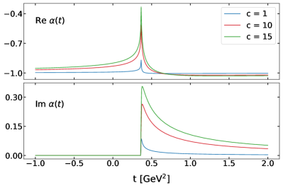
We explored a wide range of values of these two parameters and found that the trajectory depends weakly on the value of , i.e. the masses of the particles involved. Convergence of the iterative equations occurs well within ten iterations for . In Fig. 6 we show the Regge trajectory for and several values of . We find that determines the size of the peak shown in Fig. 6. Its impact in the form factor is discussed in the next section.
II.4.2 Form factor
Once the Regge trajectory is determined, the form factor can be numerically computed. First, we discuss the Reggeized form factor in Eq. 24, which is calculated using Eqs. 2 and 26. According to the results in Appendix C we have two asymptotic scenarios depending on being larger or smaller than zero. As shown in Fig. 6 the trajectory constructed in the previous subsection corresponds to the latter case, and, hence, the asymptotic behavior is
| (46) |
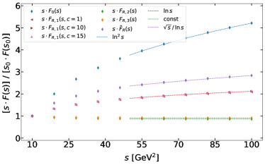
Clearly since Eq. 46 is independent of any trajectory parameters, the asymptotic behavior for any trajectory with is universal. In Fig. 7 we show the results for the numerical evaluation of the form factor for three Regge trajectories with compared to the expected asymptotic behavior. The dependence on the parameter is very mild.
For comparison purpose we also compute the form factor for a Regge trajectory that fulfills both and Eq. 44, e.g.
| (47) |
and is chosen to provide , closer to the expectation of a quark Regge trajectory. We show the result for this form factor in Fig. 7 compared to the expected high energy behavior
| (48) |
deduced in Appendix C.
Next, we compute the form factor for the Reggeized exchange and softening of one of the quark propagators as given by Eq. 27. The numerical computation shows an asymptotic behavior , which is independent of the softening power . This result is expected, and as mentioned in Section II.2, a consequence of the large momentum flowing through the perturbative propagator which leads to a nonzero 0 moment in Eq. 5. Therefore, the first term in the Eq. 4 expansion contributes, leading to the asymptotic behavior
| (49) |
III Summary and conclusions
| Pointlike | |
|---|---|
| Softened quarks | |
| Softened exchange | |
| Softened single quark | |
| Gluon exchange & softening | |
| Reggeized, | |
| Reggeized, | |
| Reggeized & softening, |
We have studied the high-energy asymptotic behavior of the electromagnetic pion form factor in simplified models to access the role of different microscopic effects. The form factor can be modeled as a triangle diagram where the photon splits into a pair who exchange a particle to produce the two pions. If all the particles and propagators are treated as scalars and the vertices as pointlike, the high energy behaviour of this model is found to be . This model sets an upper limit for the pion form factor. The rest of the models are modifications of this pointlike model and are summarized in Table 1. The inclusion of nonperturbative effects such as the pion wave function can be achieved by softening of the pair production. This modification changes the leading power, resulting in a faster fall off. However, the introduction of gluon loops effectively screen the form factor from the softening effects of the pion wave function. We also find that the inclusion of nonperturbative effects in the rescattering through the softening or the Reggeization of the exchanged particle affects the leading logarithmic correction. For the Reggeized case we find two different scenarios depending on the value of the trajectory at zero momentum transfer. The transition occurred at . This corresponds to the appearance of a spin- massless particle in the spectrum, which is not realized in nature. Nevertheless, it would be worth exploring the possibility of an enhancement of the trajectory within the context of Reggeized spin- quarks.
Acknowledgements.
CFR thanks Sean Dobbs for his insight on the CLEO-c data. This work was supported by the U.S. Department of Energy contract DE-AC05-06OR23177, under which Jefferson Science Associates, LLC operates Jefferson Lab, and DE-FG02-87ER40365, by the U.S. National Science Foundation Grant No. PHY-2310149, and by the Spanish Ministerio de Ciencia, Innovación y Universidades (MICIU) Grant Nos. PID2020-118758GB-I00 and CNS2022-136085. CFR is supported by Spanish Ministerio de Ciencia, Innovación y Universidades (MICIU) under Grant No. BG20/00133. VM is a Serra Húnter fellow. DW was supported in part by DFG and NSFC through funds provided to the Sino-German CRC 110 “Symmetries and the Emergence of Structure in QCD” (NSFC Grant No. 12070131001, DFG Project-ID 196253076). This work contributes to the aims of the U.S. Department of Energy ExoHad Topical Collaboration, contract DE-SC0023598.Appendix A Loop integrals for the softened triangle diagram
A.1 Quark propagators softened
To proceed with Eq. 13 we use Feynman parameters for positive integer . Following the conventions of Srednicki (2007), the result is
| (50) |
where
| (51) | ||||
| (52) |
For large the integral will be dominated in the region . Perform the integral in and expand around large with , and then do the same with . From this, the leading behavior is obtained to be Eq. 14.
A.2 Only the exchanged particle propagator softened
The result for softening only the exchanged quark propagator is found replacing one factor of in Eq. 13 by a factor of , replacing with , and removing one Feynman variable (or ) from the numerator
| (53) |
At large the dominant contribution to this integral is found in the region and . If one integrates Eq. 53 and expands the result in large in this region of and , the form factor is found to behave as Eq. 16.
To see the effect of altering the power of the vertical propagator as in Eq. 15 we use the dispersive technique of Section II.1. According to the delta functions attained by putting the quarks on shell, the discontinuity of the form factor becomes
| (54) |
where is the cosine of the polar angle of the loop momentum in spherical coordinates. This integral peaks when so that the denominator is not large. In this region, the dependence of the denominator is completely canceled, and it is clear that the leading behavior of form factor will not pick up any additional dependence from the integration in Eq. 2.
A.3 Only one quark propagator softened
To study the behavior of the form factor with one softened quark propagator we turn again to Feynman parameters
| (55) |
where . The dominant contribution to this integral comes from the region and . In considering the dependence of and of the numerator of Eq. 55 on the Feynman parameters, it is clear that in this region the form factor with one softened quark will fall off at most as fast as .
Appendix B Insertion of a gluon exchange
We now examine the large behavior of the gluon loop. Using Feynman parameters the gluon loop can be made to look like a propagator with dependence on the loop momentum
| (56) |
where
| (57) | ||||
| (58) |
Combining this with the other propagators in Eq. 19 and using Feynman parameters we find
| (59) |
where it is understood that . We complete the square in the loop momentum, Wick rotate, and perform the loop momentum integration to get
| (60) |
where
| (61) | ||||
| (62) |
with and that depends on the Feynman parameters and is independent of . According to the form of , the form factor will be very small unless the coefficient of is of the order or smaller in the large limit. The leading order behavior will come from the integration region and . From here it can be shown that there will remain a term with leading behavior .
Appendix C Asymptotic behavior of the Reggeized form factor
We are interested in the behavior of the integral in Eq. 26
| (63) |
We split the integral into two pieces to identify the two contributions to the large behavior
| (64) |
with . In the first integral all values of are finitely large, and the tendency of as leads to the result
| (65) |
In the second region of integration, small values of will lead to small values of . Thus we can expand around , resulting in
| (66) |
where we have made the change of variable . We note that . This integral is straightforward to evaluate
| (67) |
For we observe that , and so for large we expect Eq. 67 to be dominated by the first term in brackets. The full result at large is then
| (68) |
If () the leading behavior is the first (second) term. Considering that, as shown in Fig. 6, , the first term dominates and using Eq. 4, we obtain that the leading behavior of the form factor is
| (69) |
For a Regge trajectory with , the discontinuity at high energies reads
| (70) |
and using Eq. 4 we find
| (71) |
If the integral in Eq. 2 does not converge and it needs to be subtracted.
Appendix D Reggeized model with softening
The evaluation of Eq. 27 can be done using the relation
| (72) |
so the discontinuity can be written in terms of the th derivative
| (73) |
where
| (74) |
The discontinuity is fed into Eq. 2 to provide the form factor.
References
- Perdrisat et al. (2007) C. F. Perdrisat, V. Punjabi, and M. Vanderhaeghen, Prog. Part. Nucl. Phys. 59, 694 (2007), arXiv:hep-ph/0612014 .
- Roberts et al. (2021) C. D. Roberts, D. G. Richards, T. Horn, and L. Chang, Prog. Part. Nucl. Phys. 120, 103883 (2021), arXiv:2102.01765 [hep-ph] .
- Barabanov et al. (2021) M. Y. Barabanov et al., Prog. Part. Nucl. Phys. 116, 103835 (2021), arXiv:2008.07630 [hep-ph] .
- Li and Sterman (1992) H.-N. Li and G. F. Sterman, Nucl. Phys. B 381, 129 (1992).
- O’Connell et al. (1997) H. B. O’Connell, B. C. Pearce, A. W. Thomas, and A. G. Williams, Prog. Part. Nucl. Phys. 39, 201 (1997), arXiv:hep-ph/9501251 .
- Stefanis et al. (1999) N. G. Stefanis, W. Schroers, and H.-C. Kim, Phys. Lett. B 449, 299 (1999), arXiv:hep-ph/9807298 .
- Bakulev et al. (2004) A. P. Bakulev, K. Passek-Kumericki, W. Schroers, and N. G. Stefanis, Phys. Rev. D 70, 033014 (2004), [Erratum: Phys.Rev.D 70, 079906 (2004)], arXiv:hep-ph/0405062 .
- Gorchtein et al. (2012) M. Gorchtein, P. Guo, and A. P. Szczepaniak, Phys. Rev. C 86, 015205 (2012), arXiv:1102.5558 [nucl-th] .
- Perry et al. (2019) R. J. Perry, A. Kızılersü, and A. W. Thomas, Phys. Rev. C 100, 025206 (2019), arXiv:1811.09356 [nucl-th] .
- Brodsky and Farrar (1973) S. J. Brodsky and G. R. Farrar, Phys. Rev. Lett. 31, 1153 (1973).
- Duncan and Mueller (1980) A. Duncan and A. H. Mueller, Phys. Rev. D 21, 1636 (1980).
- Efremov and Radyushkin (1980a) A. V. Efremov and A. V. Radyushkin, Phys. Lett. B 94, 245 (1980a).
- Lepage and Brodsky (1980) G. P. Lepage and S. J. Brodsky, Phys. Rev. D 22, 2157 (1980).
- Farrar and Jackson (1979) G. R. Farrar and D. R. Jackson, Phys. Rev. Lett. 43, 246 (1979).
- Efremov and Radyushkin (1980b) A. V. Efremov and A. V. Radyushkin, Theor. Math. Phys. 42, 97 (1980b).
- Lepage and Brodsky (1979) G. P. Lepage and S. J. Brodsky, Phys. Lett. B 87, 359 (1979).
- Brown et al. (1973) C. N. Brown, C. R. Canizares, W. E. Cooper, A. M. Eisner, G. J. Feldmann, C. A. Lichtenstein, L. Litt, W. Loceretz, V. B. Montana, and F. M. Pipkin, Phys. Rev. D 8, 92 (1973).
- Bebek et al. (1976) C. J. Bebek, C. N. Brown, M. Herzlinger, S. D. Holmes, C. A. Lichtenstein, F. M. Pipkin, S. Raither, and L. K. Sisterson, Phys. Rev. D 13, 25 (1976).
- Volmer et al. (2001) J. Volmer et al. (Jefferson Lab F), Phys. Rev. Lett. 86, 1713 (2001), arXiv:nucl-ex/0010009 .
- Aul’chenko et al. (2006) V. M. Aul’chenko et al., JETP Lett. 84, 413 (2006), arXiv:hep-ex/0610016 .
- Aloisio et al. (2005) A. Aloisio et al. (KLOE), Phys. Lett. B 606, 12 (2005), arXiv:hep-ex/0407048 .
- Achasov et al. (2006) M. N. Achasov et al., J. Exp. Theor. Phys. 103, 380 (2006), arXiv:hep-ex/0605013 .
- Horn et al. (2006) T. Horn et al. (Jefferson Lab F(pi)-2), Phys. Rev. Lett. 97, 192001 (2006), arXiv:nucl-ex/0607005 .
- Tadevosyan et al. (2007) V. Tadevosyan et al. (Jefferson Lab F), Phys. Rev. C 75, 055205 (2007), arXiv:nucl-ex/0607007 .
- Horn et al. (2008) T. Horn et al., Phys. Rev. C 78, 058201 (2008), arXiv:0707.1794 [nucl-ex] .
- Akhmetshin et al. (2007) R. R. Akhmetshin et al. (CMD-2), Phys. Lett. B 648, 28 (2007), arXiv:hep-ex/0610021 .
- Aubert et al. (2009) B. Aubert et al. (BaBar), Phys. Rev. Lett. 103, 231801 (2009), arXiv:0908.3589 [hep-ex] .
- Lees et al. (2012) J. P. Lees et al. (BaBar), Phys. Rev. D 86, 032013 (2012), arXiv:1205.2228 [hep-ex] .
- Ablikim et al. (2016) M. Ablikim et al. (BESIII), Phys. Lett. B 753, 629 (2016), [Erratum: Phys.Lett.B 812, 135982 (2021)], arXiv:1507.08188 [hep-ex] .
- Ambrosino et al. (2011) F. Ambrosino et al. (KLOE), Phys. Lett. B 700, 102 (2011), arXiv:1006.5313 [hep-ex] .
- Seth et al. (2013) K. K. Seth, S. Dobbs, Z. Metreveli, A. Tomaradze, T. Xiao, and G. Bonvicini, Phys. Rev. Lett. 110, 022002 (2013), arXiv:1210.1596 [hep-ex] .
- Abdul Khalek et al. (2022) R. Abdul Khalek et al., Nucl. Phys. A 1026, 122447 (2022), arXiv:2103.05419 [physics.ins-det] .
- Accardi et al. (2023) A. Accardi et al., “Strong Interaction Physics at the Luminosity Frontier with 22 GeV Electrons at Jefferson Lab,” (2023), arXiv:2306.09360 [nucl-ex] .
- Isgur and Llewellyn Smith (1984) N. Isgur and C. H. Llewellyn Smith, Phys. Rev. Lett. 52, 1080 (1984).
- Isgur and Llewellyn Smith (1989) N. Isgur and C. H. Llewellyn Smith, Nucl. Phys. B 317, 526 (1989).
- Belyaev and Radyushkin (1996) V. M. Belyaev and A. V. Radyushkin, Phys. Rev. D 53, 6509 (1996), arXiv:hep-ph/9509267 .
- Gousset and Pire (1995) T. Gousset and B. Pire, Phys. Rev. D 51, 15 (1995), arXiv:hep-ph/9403293 .
- Fadin and Sherman (1977) V. S. Fadin and V. E. Sherman, Zh. Eksp. Teor. Fiz. 72, 1640 (1977).
- Strikman (2008) M. Strikman, Nucl. Phys. A 805, 369 (2008), arXiv:0711.1634 [hep-ph] .
- Amati et al. (1962) D. Amati, S. Fubini, and A. Stanghellini, Phys. Lett. 1, 29 (1962).
- Collins (2009) P. D. B. Collins, An Introduction to Regge Theory and High-Energy Physics, Cambridge Monographs on Mathematical Physics (Cambridge Univ. Press, Cambridge, UK, 2009).
- Eden et al. (1966) R. J. Eden, P. V. Landshoff, D. I. Olive, and J. C. Polkinghorne, The analytic -matrix (Cambridge Univ. Press, Cambridge, 1966).
- Roberts (2015) C. D. Roberts, IRMA Lect. Math. Theor. Phys. 21, 355 (2015), arXiv:1203.5341 [nucl-th] .
- Gell-Mann et al. (1964) M. Gell-Mann, M. Goldberger, F. Low, E. Marx, and F. Zachariasen, Phys. Rev. 133, B145 (1964).
- Chew and Mandelstam (1960) G. F. Chew and S. Mandelstam, Phys. Rev. 119, 467 (1960).
- Londergan et al. (2014) J. T. Londergan, J. Nebreda, J. R. Peláez, and A. Szczepaniak, Phys. Lett. B 729, 9 (2014), arXiv:1311.7552 [hep-ph] .
- Peláez and Rodas (2017) J. R. Peláez and A. Rodas, Eur. Phys. J. C 77, 431 (2017), arXiv:1703.07661 [hep-ph] .
- Blankenbecler et al. (1973) R. Blankenbecler, S. J. Brodsky, J. F. Gunion, and R. Savit, Phys. Rev. D 8, 4117 (1973).
- Srednicki (2007) M. Srednicki, Quantum field theory (Cambridge University Press, 2007).