Charged scalar bosons in a Bonnor-Melvin-$\Lambda$ universe at conical approximation

Abstract

The quantum dynamics of charged scalar bosons in a Bonnor-Melvin-$\Lambda$ universe is considered. In this study, the behavior of charged scalar bosons is explored within the framework of the Duffin-Kemmer-Petiau (DKP) formalism. Adopting a conical approximation ($\Lambda\ll 1$), we are considered two scenarios for the vector potential: a linear and quadratic vector potentials. In particular, the effects of this background in the equation of motion, phase shift, $S$-matrix, energy spectrum and DKP spinor are analyzed and discussed.

1 Introduction

The first-order Duffin-Kemmer-Petiau (DKP) formalism Petiau1936 ; Kemmer1938 ; PR54:1114:1938 ; Kemmer1939 is employed to describe spin-zero and spin-one particles. It has been utilized to examine relativistic interactions between spin-zero and spin-one hadrons and nuclei, providing an alternative to their conventional second-order counterparts, the Klein-Gordon (KG) and Proca equations. While these formalisms are equivalent in the case free and involving minimally coupled vector interactions PLA244:329:1998 ; PLA268:165:2000 ; PRA90:022101:2014 , it is worth emphasizing that the DKP formalism offers a broader range of coupling possibilities that cannot be expressed within the confines of the Klein-Gordon (KG) and Proca theories PRD15:1518:1977 ; JPA12:665:1979 .

Solutions of the DKP equation in curved space-time have been obtained for many systems and have been studied extensively in the literature in recent years EPJC44:287:2005 ; IJMPA25:2747:2010 ; AP343:40:2014 ; EPJP130:236:2015 ; EPJC75:287:2015 ; EPJC76:61:2016 ; EPJP132:541:2017 ; EPL118:10002:2017 ; EPJC78:93:2018 ; GRG50:104:2018 ; IJMPA34:1950056:2019 ; IJMPA34:1950082:2019 ; GRG52:25:2020 ; IJMPA35:2050107:2020 ; MPLA36:2150059:2021 ; IJMPE30:2150050:2021 ; CQG39:075007:2022 ; PS98:065224:2023 ; FBS64:13:2023 . In these references, the authors are considered various models of curved space-time and investigated the effects of such backgrounds on the energies of bound states of DKP particles. These investigations are significant as they explore the relationship between curved space-time and relativistic particle dynamics. They provide valuable insights into the fundamental nature of the universe by studying the behavior of particles in extreme gravitational environments such as black holes and cosmological structures.

Magnetic fields are crucial in understanding various astrophysical phenomena across different distance scales, from stars to intergalactic regions. They shape celestial dynamics, influence accretion disks around black holes, and regulate processes in galactic nuclei. Even on large scales, magnetic fields impact cosmic matter distribution. Incorporating the magnetic field into the metric is not a trivial matter, but some solutions have been proposed. Notable examples include the Bonnor-Melvin metric PPSA67:225:1954 ; PL8:65:1964 , which describes a magnetic universe with a magnetic field aligned in the $z$-direction, and the Gutsunaev solution PLA123:215:1987 ; PLA132:85:1988 , which refers to a magnetic dipole. A theoretical description of fermions and bosons in a Bonnor-Melvin metric has been addressed in recent literature EPJC76:560:2016 ; ADHEP2018:1953586:2018 . In these work, fermions and scalar bosons are described by the Dirac and Klein-Gordon (KG) formalisms, respectively. Currently, this is an open problem that deserves further exploration.

The Bonnor-Melvin universe, as presented in references PPSA67:225:1954 ; PL8:65:1964 , represents an exact solution to the Einstein-Maxwell equations. This solution characterizes a static, cylindrically symmetric (electro)magnetic field immersed within its own gravitational field. The magnetic field is aligned with the symmetry axis, but it is not homogeneous. Recently, as demonstrated in PRD99:044058:2019 , the author extended the Bonnor-Melvin solution to encompass a nonvanishing cosmological constant (Bonnor-Melvin-$\Lambda$ universe). In this setting, the space-time maintains its cylindrical symmetric and static nature, but, unlike the original solution, it genuinely represents a homogeneous magnetic field (intrinsic). A theoretical description of scalar bosons in a Bonnor-Melvin-$\Lambda$ universe has been addressed in barbosa2023scalar . The authors are solved the KG equation and determined the Landau levels for the case free and for a Coulomb-like scalar potential. However, the investigation of scalar bosons in a Bonnor-Melvin-$\Lambda$ universe using the DKP formalism remains uncharted territory. Hence, we believe that this unexplored problem holds significant potential for further study.

Inspired by these studies, we explore the dynamics of a charged scalar boson using the DKP formalism immersed in a Bonnor-Melvin-$\Lambda$ universe. Our analysis examines the effects of both the intrinsic magnetic field and an additional external magnetic field associated with a four-vector potential $A_{\mu}$, which is minimally coupled. We aim to examine the quantum effects associated with gravitation from the perspective of relativistic quantum mechanics in curved spacetime. To achieve this, we analyze the scalar sector of the DKP equation in this context and derive the equation of motion for an arbitrary form of the vector potential. Given the complexity of the equation of motion, we employed the approximation $\sqrt{2\Lambda}r\ll 1$, or equivalently, $\Lambda\ll 1$, enabling us to examine the influence of the Bonnor-Melvin-$\Lambda$ model parameters through an analytical expression for the eigenfunctions. Here, we consider two scenarios for the vector potential: a linear and quadratic vector potentials. The problem is mapped into a Schrödinger-like equation for the first component of the DKP spinor with a Coulomb-like potential (linear vector potential) and harmonic oscillator (quadratic vector potential). The remaining components are expressed in terms of the one in a simple way. For the linear vector potential, the equation of motion, phase shift and scattering $S$-matrix are calculated from a Whittaker differential equation via partial wave analysis. The bound-state solutions are obtained from the poles of the $S$-matrix and the restriction on the potential parameters are discussed in detail. For the quadratic vector potential, the equation of motion and bound-state solutions are calculated from a confluent hypergeometric differential equation. In both scenarios, the first component of the DKP spinor is expressed in terms of the generalized Laguerre polynomial and the energy spectrum is composed of particle and antiparticle energies, and it is symmetrical about $E=0$.

This work is organized as follows. In section 2, we give a brief review on DKP equation in a curved space-time. In section 3, we analyse the minimal coupling, the condition on the beta matrices which lead to a conserved current in a curved space-time, and the normalization condition for the DKP formalism. In the section 4, we focus in the DKP equation with minimal coupling in a Bonnor-Melvin-$\Lambda$ universe. Adopting the limit $\Lambda\ll 1$, we discuss in detail the problem considering two scenarios for the vector potential: linear potential (section 4.1) and quadratic potential (section 4.2). Finally, in section 5 we present our conclusions.

2 Review of Duffin-Kemmer-Petiau equation in a curved space-time

The Duffin-Kemmer-Petiau (DKP) equation for a free boson in curved space-time is given by GRG34:491:2002 ; GRG34:1941:2002 ; EPJC75:287:2015 ; EPJC76:61:2016 ($\hbar=c=1$)

$$\left(i\beta^{\mu}\nabla_{\mu}-M\right)\Psi=0$$ (1)

where the covariant derivative

$$\nabla_{\mu}=\partial_{\mu}-\Gamma_{\mu}\,.$$ (2)

We restrict our study to the torsion-zero and the affine connection is defined by

$$\Gamma_{\mu}=\frac{1}{2}\,\omega_{\mu\bar{a}\bar{b}}[\beta^{\bar{a}},\beta^{\bar{b}}]\,.$$ (3)

The curved-space beta matrices are

$$\beta^{\mu}=e^{\mu}\,_{\bar{a}}\,\beta^{\bar{a}}$$ (4)

and satisfy the algebra

$$\beta^{\mu}\beta^{\nu}\beta^{\lambda}+\beta^{\lambda}\beta^{\nu}\beta^{\mu}=g^{\mu\nu}\beta^{\lambda}+g^{\lambda\nu}\beta^{\mu}\,.$$ (5)

where $g^{\mu\nu}$ is the metric tensor. The algebra represented by (5) gives rise to a set of 126 independent matrices, which can be classified into irreducible representations. These representations include a trivial representation, a five-dimensional representation that describes spin-zero particles (scalar sector), and a ten-dimensional representation associated to spin-one particles (vector sector). For the purposes of this discussion, we concentrate our attention on the spin-$0$ sector of the DKP theory.

The tetrads $e_{\mu}\,^{\bar{a}}(x)$ satisfy the relations

$$\eta^{\bar{a}\bar{b}}=e_{\mu}\,^{\bar{a}}\,e_{\nu}\,^{\bar{b}}\,g^{\mu\nu}$$ (6)

$$g_{\mu\nu}=e_{\mu}\,^{\bar{a}}\,e_{\nu}\,^{\bar{b}}\,\eta_{\bar{a}\bar{b}}$$ (7)

and

$$e_{\mu}\,^{\bar{a}}\,e^{\mu}\,_{\bar{b}}=\delta^{\bar{a}}_{\bar{b}}$$ (8)

the Latin indexes being raised and lowered by the Minkowski metric tensor $\eta^{\bar{a}\bar{b}}$ with signature $(-,+,+,+)$ and the Greek ones by the metric tensor $g^{\mu\nu}$.

The spin connection $\omega_{\mu\bar{a}\bar{b}}$ is given by

$$\omega_{\mu}\,^{\bar{a}\bar{b}}=e_{\alpha}\,^{\bar{a}}\,e^{\nu\bar{b}}\,\Gamma_{\mu\nu}^{\alpha}-e^{\nu\bar{b}}\partial_{\mu}e_{\nu}\,^{\bar{a}}$$ (9)

with $\omega_{\mu}\,^{\bar{a}\bar{b}}=-\omega_{\mu}\,^{\bar{b}\bar{a}}$ and $\Gamma_{\mu\nu}^{\alpha}$ are the Christoffel symbols given by

$$\Gamma_{\mu\nu}^{\alpha}=\frac{g^{\alpha\beta}}{2}\left(\partial_{\mu}g_{\beta\nu}+\partial_{\nu}g_{\beta\mu}-\partial_{\beta}g_{\mu\nu}\right).$$ (10)

More detailed discussions on the DKP formalism in a curved space-time can be found in Ref. EPJC75:287:2015 .

3 Interactions in the DKP equation

The DKP equation for a charged scalar boson in curved space-time is given by

$$\left[i\beta^{\mu}\left(\nabla_{\mu}+iqA_{\mu}\right)-M\right]\Psi=0\,.$$ (11)

As it is shown in Ref. EPJC75:287:2015 , the conservation law for $J^{\mu}$ with interaction is given by

$$\nabla_{\mu}J^{\mu}=\frac{1}{2}\bar{\Psi}\left(\nabla_{\mu}\beta^{\mu}\right)\Psi$$ (12)

where $J^{\mu}=\frac{1}{2}\bar{\Psi}\beta^{\mu}\Psi$. It is worthwhile to mention that the interactions $\beta^{\mu}A_{\mu}$ is Hermitian with respect to $\eta^{0}$, with $\eta^{0}=2\beta^{0}\beta^{0}-1$ (the matrices $\beta^{\mu}$ are Hermitian with respect to $\eta^{0}$, $(\eta^{0}\beta^{\mu})^{{\dagger}}=\eta^{0}\beta^{\mu}$). Furthermore, if

$$\nabla_{\mu}\beta^{\mu}=0$$ (13)

then four-current will be conserved EPJC75:287:2015 ; EPJC76:61:2016 . The condition (13) is the purely geometrical assertion that the curved-space beta matrices are covariantly constant.

The normalization condition $\int{d\tau J^{0}}=\pm 1$ can be expressed as

$$\int{d\tau\bar{\Psi}\beta^{0}\Psi}=\pm 2\,,$$ (14)

where the plus (minus) sign must be used for a positive (negative) charge. Furthermore, the expectation value of any observable $\mathcal{O}$ can be given by

$$\langle\mathcal{O}\rangle=\frac{\int d\tau\bar{\Psi}\beta^{0}\mathcal{O}\Psi}{\int d\tau\bar{\Psi}\beta^{0}\Psi}\,,$$ (15)

where $\beta^{0}\mathcal{O}$ should be Hermitian with respect to $\eta^{0}$, $\left[\eta^{0}\left(\beta^{0}\mathcal{O}\right)\right]^{\dagger}=\eta^{0}\left(\beta^{0}\mathcal{O}\right)$, in order to provide real eigenvalues PRA90:022101:2014 .

4 DKP equation in a Bonnor-Melvin-$\Lambda$ universe

The Bonnor-Melvin-$\Lambda$ solution of the Einstein-Maxwell equations to the case of a nonvanishing cosmological constant is described by the line element PRD99:044058:2019

$$ds^{2}=-dt^{2}+dr^{2}+\sigma^{2}\sin^{2}\left(\sqrt{2\Lambda}r\right)d\varphi^{2}+dz^{2}\,,$$ (16)

in cylindrical coordinates $(t,r,\varphi,z)$, where $-\infty<z<+\infty$, $r\geq 0$ and $0\leq\varphi\leq 2\pi$. The parameter $\sigma$ is a integration constant and $\Lambda$ is the cosmological constant. The Ricci scalar curvature corresponding to this metric is $R=4\Lambda$. This demonstrates that the spacetime described by the metric (16) is not asymptotically flat; instead, it displays a uniform curvature across the universe.

On the other hand, this line element reflects the curvature of spacetime determined by the following periodic magnetic field aligned with the axis of symmetry

$$H(r)=\sqrt{\Lambda}\sigma\sin\left(\sqrt{2\Lambda}r\right).$$ (17)

The basis tetrad $e^{\mu}\,_{\bar{a}}$ from the line element (16) is chosen to be

$$e^{\mu}\,_{\bar{a}}=\begin{pmatrix}1&0&0&0\\ 0&1&0&0\\ 0&0&\frac{1}{\sigma\sin\left(\sqrt{2\Lambda}r\right)}&0\\ 0&0&0&1\end{pmatrix}\,.$$ (18)

For the specific basis tetrad (18) the curved-space beta matrices read

$$\beta^{0} = \beta^{\bar{0}}\,,$$ (19)

$$\beta^{r} = \beta^{\bar{1}}\,,$$ (20)

$$\beta^{\varphi} = \frac{1}{\sigma\sin\left(\sqrt{2\Lambda}r\right)}\beta^{\bar{2}}\,,$$ (21)

$$\beta^{z} = \beta^{\bar{3}}\,,$$ (22)

and the spin connection is given by

$$\Gamma_{\varphi}=-\sqrt{2\Lambda}\sigma\cos\left(\sqrt{2\Lambda}r\right)\left[\beta^{\bar{1}},\beta^{\bar{2}}\right]\,.$$ (23)

Thereby, the covariant derivative gets

$$\nabla_{0} = \partial_{0}\,,$$ (24)

$$\nabla_{r} = \partial_{r}\,,$$ (25)

$$\nabla_{\varphi} = \partial_{\varphi}+\sqrt{2\Lambda}\sigma\cos\left(\sqrt{2\Lambda}r\right)\left[\beta^{\bar{1}},\beta^{\bar{2}}\right]\,,$$ (26)

$$\nabla_{z} = \partial_{z}$$ (27)

At this stage, note that the condition (13) is satisfied for the curved-space beta matrices (19), (20), (21) and (22) and therefore the current is conserved for this background.

Following the expressions presented above, we now study the dynamics of a charged scalar boson in a Bonnor-Melvin-$\Lambda$ universe in the presence of an additional magnetic field. To accomplish this, we consider a four-vector potential, $A_{\mu}$, in curved space associated with this external field. This potential is defined as $A_{\mu}=e_{\mu}{}^{\bar{a}}A_{\bar{a}}$, where $A_{\bar{a}}$ represents the four-vector potential in flat space-time oliveira2020noninertial ; huamani2022aharonov ; soares2023effects . In this case, we consider $A_{\bar{a}}$ in the form

$$A_{\bar{a}}=(0,0,A_{\bar{2}},0)=(0,0,-f(r),0),$$ (28)

where $f(r)$ is the functional form of the four-vector potential in the flat space-time. The choice of this structure for $A_{\bar{a}}$ was driven by the goal of preserving the axial symmetry of the Bonnor-Melvin-$\Lambda$ universe. Furthermore, this configuration facilitates the derivation of analytical solutions under the approximation described in this work. We will discuss this approach in more detail later.

By using the inverse tetrad $e_{\varphi}\,^{\bar{2}}=\sigma\sin\left(\sqrt{2\Lambda}r\right)$, the four-vector potential in the Bonnor-Melvin-$\Lambda$ universe is defined as

$$A_{\varphi}=\sigma\sin\left(\sqrt{2\Lambda}r\right)f(r)\,.$$ (29)

As the interaction is time-independent, we can express $\Psi(\vec{r},t)=\Phi(\vec{r})\mathrm{exp}\left(-iEt\right)$ in equation (11), where $E$ represents the energy of the scalar boson. Consequently, the time-independent DKP equation transforms into

$$\left[\beta^{\bar{0}}E+i\beta^{\bar{1}}\partial_{r}+i\beta^{\varphi}\nabla_{\varphi}+\beta^{\varphi}A_{\varphi}+i\beta^{\bar{3}}\partial_{z}-M\right]\Phi=0\,,$$ (30)

where $\beta^{\varphi}$, $\nabla_{\varphi}$ and $A_{\varphi}$ are given by (21), (26) and (29), respectively. We now adopt the standard representation for the beta matrices as described in JPG19:87:1993 . With the five-component spinor $\Phi^{T}=(\Phi_{1},\ldots,\Phi_{5})$, the time-independent DKP equation (30) becomes

$$E\Phi_{2} - M\Phi_{1}-i\bar{\partial}_{r}\Phi_{3}-i\bar{\partial}_{\varphi}\Phi_{4}-i\partial_{z}\Phi_{5}=0\,,$$ (31)

$$\Phi_{2} = \frac{E}{M}\Phi_{1}\,,$$ (32)

$$\Phi_{3} = \frac{i}{M}\partial_{r}\Phi_{1}\,,$$ (33)

$$\Phi_{4} = \frac{i}{M}\bar{\partial}_{\varphi}\Phi_{1}\,,$$ (34)

$$\Phi_{5} = \frac{i}{M}\partial_{z}\Phi_{1}\,,$$ (35)

where

$$\bar{\partial}_{r} = \partial_{r}+\frac{\sqrt{2\Lambda}}{\tan\left(\sqrt{2\Lambda}r\right)}\,,$$ (36)

$$\bar{\partial}_{\varphi} = \frac{\partial_{\varphi}}{\sigma\sin\left(\sqrt{2\Lambda}r\right)}-iqf(r)\,.$$ (37)

Nonetheless,

$$J^{0}=\mathrm{Re}\left(\Phi_{2}^{\ast}\Phi_{1}\right)=\frac{E}{M}|\Phi_{1}|^{2}\,.$$ (38)

By combining these outcomes, we establish an equation of motion governing the first component of the DKP spinor

$$\begin{split}&\left[\partial^{2}_{r}+\frac{\sqrt{2\Lambda}}{\tan\sqrt{2\Lambda}r}\partial_{r}+\frac{1}{\sigma^{2}\sin^{2}\sqrt{2\Lambda}r}\partial^{2}_{\varphi}+\partial^{2}_{z}\right.\\ &\left.-q^{2}f^{2}(r)-\frac{2iqf(r)}{\sigma\sin\sqrt{2\Lambda}r}\partial_{\varphi}+E^{2}-M^{2}\right]\Phi_{1}=0\,.\end{split}$$ (39)

Given the complexity of equation (39), we adopted an approach that allows us to analyze the impact of the Bonnor-Melvin-$\Lambda$ model parameters on scalar boson dynamics using analytical solutions for $\Phi_{1}$. We explain our reasoning as follows.

As mentioned earlier, our investigation focused on examining the quantum effects associated with gravitation from the perspective of relativistic quantum mechanics in curved spacetimes. Several studies have been instrumental in exploring these effects, including the use of the Dirac dariescu2021dirac and Klein-Gordon vieira2014exact equations in Kerr-Newman space, as well as the Dirac equation in Robertson-Walker spacetime barut1987exact , among others. Nonetheless, one aspect that has not received enough attention in this context is related to distance scales. In the context of the Bonnor-Melvin-$\Lambda$ universe, it becomes particularly interesting to examine specific spatial regions where the order of magnitude of spatial coordinate $r$ is inversely proportional to the order of magnitude of $\sqrt{\Lambda}$. This proportionality plays a crucial role in preserving the effects of the cosmological constant $\Lambda$ and ensuring the periodic behavior of both the metric and the magnetic field, due to the presence of the term $\sin(\sqrt{2\Lambda}r)$. This approach was utilized in the works of Žofka in the context of general relativity, as detailed in references PRD99:044058:2019 , vesely2021cylindrical , and vesely2022exact . In this manner, the cosmological constant $\Lambda$ effectively controls the order of magnitude of cosmological distances, manifesting its influence at such scales.

Nevertheless, our work focuses on a quantum scenario, rather than a cosmological one. That is, the spatial coordinate $r$ is at a microscopic scale. Consequently, the cosmological constant is no longer capable of controlling the order of magnitude of the argument of the sine, making the product $\sqrt{2\Lambda}r$ very small, or, equivalently, $\Lambda\ll 1$. The plausibility of a small cosmological constant has been considered in various scenarios at quantum scale, including non-supersymmetric theories with a light dilaton EPJC74:2790:2014 , 5D brane world models JHEP2017:71:2017 , and supersymmetric string theory GRG40:607:2008 ; PRL128:011602:2022 , among others.

It is noteworthy that this condition naturally supports the approximation $\sin(\sqrt{2\Lambda}r)\approx\sqrt{2\Lambda}r$, allowing the metric (16) to be reexpressed as

$$ds^{2}=-dt^{2}+dr^{2}+2\Lambda\sigma^{2}r^{2}d\varphi^{2}+dz^{2},$$ (40)

where the Ricci scalar curvature is now given by $R=\delta(r)$. This implies that the curvature in this metric is null everywhere except at the point where the source is located $(r=0)$, resembling the spacetime generated by a cosmic string EPJC75:287:2015 . From the latter, one can infer that the metric (40) describes a spacetime with a conical singularity generated by the term $2\Lambda\sigma^{2}$ at $r=0$ sokolov1977structure . Furthermore, the line element (40) produces a magnetic field aligned with the axis of symmetry given by

$$H(r)=\sqrt{2}\Lambda\sigma r\,,$$ (41)

and the four-vector potential in the Bonnor-Melvin-$\Lambda$ universe (29) reduces to

$$A_{\varphi}=\sqrt{2\Lambda}\sigma rf(r)\,.$$ (42)

Therefore, in this approximation, the equation (39) becomes

$$\begin{split}&\left[\partial^{2}_{r}+\frac{1}{r}\partial_{r}+\frac{1}{H_{0}^{2}r^{2}}\partial^{2}_{\varphi}+\partial^{2}_{z}-q^{2}f^{2}(r)\right.\\ &\left.-\frac{2iqf(r)}{H_{0}r}\partial_{\varphi}+E^{2}-M^{2}\right]\Phi_{1}=0\,,\end{split}$$ (43)

where $H_{0}=\sqrt{2\Lambda}\sigma$. At this point, we can leverage the invariance under boosts along the $z$-direction and proceed with the standard decomposition:

$$\Phi_{1}(r,\varphi,z)=\frac{\phi_{1}(r)}{\sqrt{r}}e^{im\varphi+ik_{z}z}$$ (44)

with $m\in\mathbb{Z}$. Inserting this into Eq. (43), we obtain

$$\begin{split}&\left[\frac{d^{2}}{dr^{2}}-\frac{\left(m_{\Lambda}^{2}-\frac{1}{4}\right)}{r^{2}}-q^{2}f^{2}(r)\right.\\ &\left.+\frac{2qm_{\Lambda}f(r)}{r}+E^{2}-M^{2}-k_{z}^{2}\right]\phi_{1}=0\,,\end{split}$$ (45)

where $m_{\Lambda}=\frac{m}{H_{0}}$. Now, we can apply the framework developed above to solve the DKP equation in this background, utilizing specific forms for $f(r)$. The choice of $f(r)$ is justified by the magnetic field produced by the four-vector potential, which is expected to be uniform as indicated in reference vallee2004cosmic .

4.1 Linear interaction

Considering $f(r)=\frac{\alpha_{1}}{2}$, where $\alpha_{1}$ is a constant, this particular form of $f(r)$ leads to $A_{\varphi}=\frac{\alpha_{1}H_{0}r}{2}$ (linear interaction), which furnish a magnetic field $\vec{B}=\frac{\alpha_{1}}{2r}\hat{z}$. In this scenario, the equation (45) becomes

$$\left[-\frac{d^{2}}{dr^{2}}-\frac{\delta}{r}+\frac{\left(m_{\Lambda}^{2}-\frac{1}{4}\right)}{r^{2}}-\kappa^{2}\right]\phi_{1}=0\,,$$ (46)

where $\delta=qm_{\Lambda}\alpha_{1}$ and

$$\kappa=\sqrt{E^{2}-M^{2}-k_{z}^{2}-\frac{q^{2}\alpha_{1}^{2}}{4}}\,.$$ (47)

Equation (46) characterizes the relativistic motion of charged scalar bosons that interact with a linear vector potential within the framework of a Bonnor-Melvin-$\Lambda$ universe. With $\phi_{1}(0)=0$ and $\int_{0}^{\infty}|\phi_{1}|^{2}dr<\infty$, this equation exactly corresponds to the time-independent radial Schrödinger equation for a Coulomb-like potential in two dimensions. The potential exhibits a well structure when $\delta>0$, which implies that $m_{\Lambda}\alpha_{1}>0$. Additionally, bound states are expected for $\kappa=i|\kappa|$, i.e. $-\varepsilon<E<+\varepsilon$, with

$$\varepsilon=\sqrt{M^{2}+k_{z}^{2}+\frac{q^{2}\alpha_{1}^{2}}{4}}\,.$$ (48)

Therefore, we can conclude that bound-state solutions might occur only for $m_{\Lambda}\alpha_{1}>0$, corresponding to energies in the interval $-\varepsilon<E<+\varepsilon$. On the other hand, the solution $\phi_{1}(r)$ has asymptotic behavior $\mathrm{e}^{\pm i\kappa r}$, so we can expect that scattering states only occur if $\kappa\in\mathbb{R}$, i.e. $|E|>\varepsilon$.

After conducting a qualitative analysis of the effective potential, we will be able to develop a quantitative approach to our problem by examining the bound-state solutions, which are obtained from the poles of the S-matrix, and the restrictions on the potential parameters of the system. This will be discussed in detail in the following section.

4.1.1 Scattering states and the $S$-matrix

Using the abbreviation

$$\eta=\frac{\delta}{2\kappa},$$ (49)

and the change $\rho=-2i\kappa r$, the equation (46) becomes

$$\frac{d\phi_{1}}{d\rho^{2}}+\left(-\frac{1}{4}+\frac{i\eta}{\rho}+\frac{\frac{1}{4}-m_{\Lambda}^{2}}{\rho^{2}}\right)\phi_{1}=0.$$ (50)

This second-order differential equation is the called Whittaker equation. Owing to the condition $\phi_{1}(0)=0$, only the regular solution at the origin is allowed. In this case, the solution is given by

$$\phi_{1}\propto\rho^{|m_{\Lambda}|+1/2}e^{-\rho/2}M\left(a,b;\rho\right)\,,$$ (51)

where

$$a = |m_{\Lambda}|-i\eta+\frac{1}{2}\,,$$ (52)

$$b = 1+2|m_{\Lambda}|\,,$$ (53)

and $M(a,b;\rho)$ is the Kummer’s function, whose asymptotic behavior for large $|\rho|$ with a purely imaginary $\rho=-i|\bar{\rho}|$, where $|\bar{\rho}|=2\kappa r$ is given by JAMES1991

$$\begin{split}M(a,b;\rho)&\simeq\frac{\Gamma(b)}{\Gamma(a-b)}e^{-\frac{i\pi a}{2}}|\bar{\rho}|^{-a}\\ &+\frac{\Gamma(b)}{\Gamma(a)}e^{-i[|\bar{\rho}|-\frac{\pi(b-a)}{2}]}|\bar{\rho}|^{a-b}.\end{split}$$ (54)

Using this last result, we can show that for $|\rho|\gg 1$ and $\kappa\in\mathbb{R}$, the asymptotic behavior of (51) is given by AP146:1:1983

$$\phi(r)\simeq\cos\left(\kappa r-\frac{|m|\pi}{2}-\frac{\pi}{4}+\delta_{m}\right),$$ (55)

where the relativistic phase shift $\delta_{m}=\delta_{m}(\eta)$ is given by

$$\delta_{m}=\frac{\pi}{2}(|m|-|m_{\Lambda}|)+\text{arg}\Gamma\left(\frac{1}{2}+|m_{\Lambda}|-i\eta\right)\,.$$ (56)

From this last expression, we can express the scattering $S$-matrix as

$$S_{m}=\mathrm{e}^{2i\delta_{m}}=\mathrm{e}^{i\pi(|m|-|m_{\Lambda}|)}\frac{\Gamma\left(1/2+|m_{\Lambda}|-i\eta\right)}{\Gamma\left(1/2+|m_{\Lambda}|+i\eta\right)}\,.$$ (57)

The distribution of points in the complex plane of the $S$-matrix is shown in figure 1, with the following parameters PRD97:076008:2018 : with $m=1$, $q=1$, $M=0.14$ GeV, $k_{z}=0.14$ GeV, $\alpha_{1}=0.30$ GeV, $\sigma=1$ and $\Lambda=0.011$ (panel a), $\Lambda=0.045$ (panel b) and $\Lambda=0.080$ (panel c) (expressed in natural units).

The red points in Fig. 1 represent the poles of the $S$-matrix, which are infinite in number and located on the imaginary axis of $\kappa$ (where $\mathrm{Re}(\kappa)=0$). These poles occur only for non-negative integer values of the argument of the gamma function in the numerator of equation (57). In each panel, the $\kappa$ values associated with an $S$-matrix pole exhibit a maximum at the zeroth-order pole, which is given by $\kappa_{max}=i\delta/(1+2|m_{\Lambda}|)$. Note that the spacing between the poles decreases progressively as higher-order poles are observed. Notably, as $\Lambda$ increases ($|m_{\Lambda}|$ decreases), these poles tend to shift towards $\mathrm{Im}(\kappa)=0$, leading to an increase in the concentration of poles in the regions of the higher-order poles. For this reason, Fig. 1 specifically selects an interval of

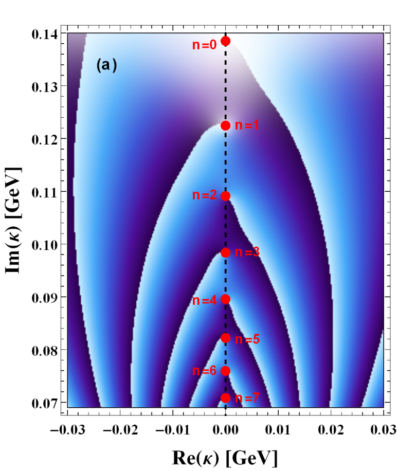
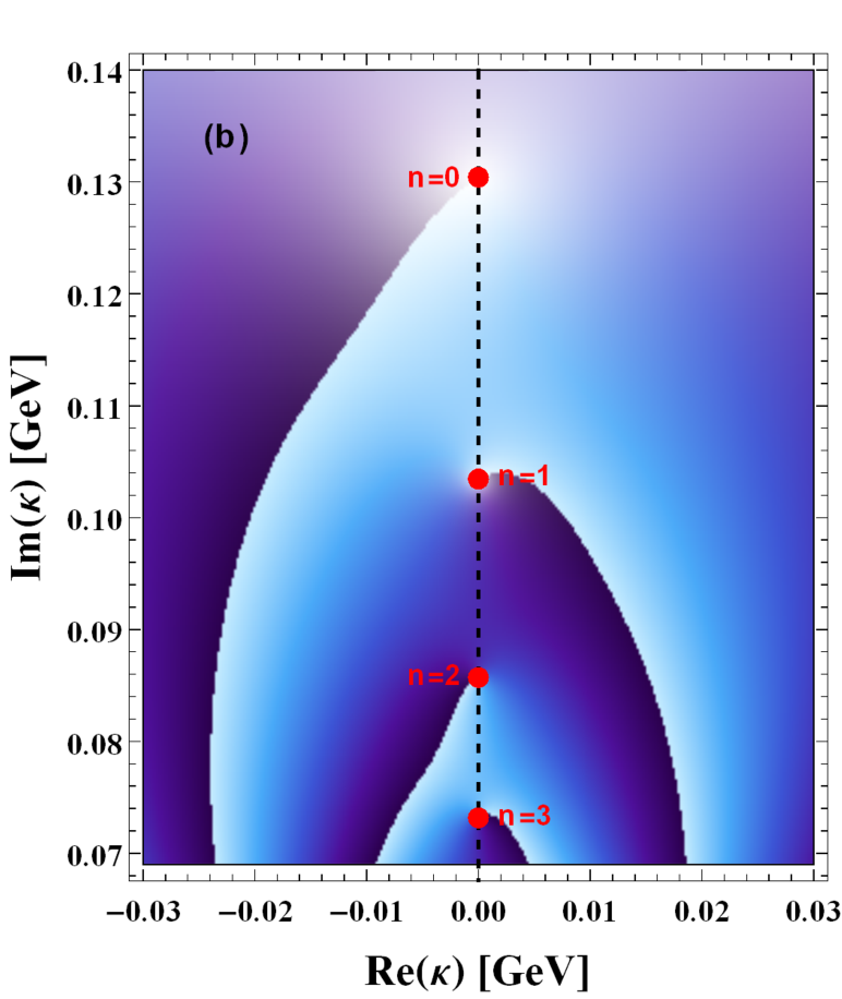
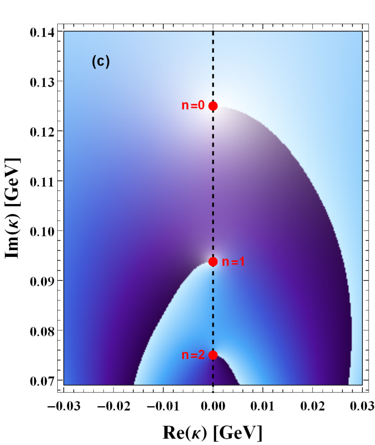
Figure 1: Plot of the $S$-matrix as a function of the real and imaginary part of $\kappa$ for $\Lambda=0.011$ (panel a), $\Lambda=0.045$ (panel b) and $\Lambda=0.080$ (panel c) (expressed in natural units).

$\mathrm{Im}(\kappa)$ from $0.07$ to $0.14$ on the gigascale for each panel, allowing for a clear visualization of this redistribution of the poles as the cosmological constant $\Lambda$ varies. A high concentration of poles is associated with the so-called accumulation point of states, which is a distinctive feature in systems with Coulomb-like interactions that exhibit an infinite number of states below a certain energy. This observation is crucial in the next section, where we establish that the presence of these poles in the $S$-Matrix leads to the quantization condition for bound-state solutions, as discussed in castro2017relativistic ; neto2020scalar .

4.1.2 Bound states

The energies of the bound-state solutions can be obtained from poles of the $S$-matrix when one considers $\kappa$ imaginary. Then, if $\kappa=i|\kappa|$, the $S$-matrix becomes infinite when $1/2+|m_{\Lambda}|-i\eta=-n$, where $n=0,1,2,\ldots$, owing to the poles of the gamma function in the numerator of (57). As previously indicated, bound-state solutions are possible only for $m_{\Lambda}\alpha_{1}>0$, corresponding to energies in the interval $-\varepsilon<E<+\varepsilon$ and the spectrum is given by

$$E=\pm\sqrt{M^{2}+k_{z}^{2}+\frac{q^{2}\alpha_{1}^{2}}{4}-\frac{q^{2}\alpha_{1}^{2}m_{\Lambda}^{2}}{4\mu^{2}}}\,,$$ (58)

with $\mu=n+1/2+|m_{\Lambda}|$. Note that the energy spectrum, comprising both particle energy (positive) and antiparticle energy (negative), is symmetrical about $E=0$, indicating that this scenario does not distinguish between particles and antiparticles. Furthermore, the energy spectrum (58) features an infinite number of bound states, with each successive pair of energies being closer together than the previous pair. This means that sufficiently high pairs of energy levels approach spacing near zero. In this region of the spectrum, the effects of energy discretization diminish, thereby bringing the system closer to the so-called accumulation point of states as $E\rightarrow\varepsilon$, occurring when $n\rightarrow\infty$. This accumulation point establishes the threshold between the spectrum of bound states and scattering states, which is a characteristic of systems with Coulomb-like interactions. In this scenario, the cosmological constant acts as a control parameter, accelerating the accumulation of states as $\Lambda$ increases ($m_{\Lambda}$ decreases), and vice versa. This finding is consistent with the results shown in Fig. 1, where the concentration of poles increases as $\sqrt{2\Lambda}\sigma$ increases.

On the other hand, in Fig. 2 we illustrate the energy distribution $|E|$ for bound states as a function of the quantum numbers $n$ and $m$, with $q=1$, $M=0.14$ GeV, $k_{z}=0.14$ GeV, $\sigma=1$, $\Lambda=0.80$ and $\alpha_{1}=0.30$ GeV (expressed in natural units). At this point, we would like to highlight three specific situations. In the case, when $n\gg m$, the energies of bound states converge to approximately $0.24$  GeV in regions near the vertical axis. This energy value corresponds to the upper threshold defined in (48). Conversely, when $n/m\approx 1$ (along the diagonal of the figure), we can observe that the energies cluster around $0.22$   GeV, remaining fixed regardless of the values of $n$ and $m$.

Finally, in the situation when $n\ll m$, the energies reach their lowest value of approximately $0.20$ in regions near the horizontal axis. The solution for all $r$ can be written as

$$\phi_{1}(\rho)=N_{n}r^{|m_{\Lambda}|+1/2}\mathrm{e}^{-|\kappa|r}L^{(2|m_{\Lambda}|)}_{n}(2|\kappa|r)\,,$$ (59)

due to $M(-n,b;\rho)$ with $b>0$ is proportional to the generalized Laguerre polynomial $L^{(b-1)}_{n}(\rho)$ ABRAMOWITZ1965 , a polynomial of degree $n$ with $n$ distinct positive zeros in the range $[0,\infty)$. The normalization constant $N_{n}$ in (59) is obtained by means of the normalization condition. The charge density $J^{0}$ (38) implies that $\phi_{1}$ must be normalized as

$$\frac{|E|}{M}\int dr|\phi_{1}|^{2}=1\,.$$ (60)

In this way, the normalization constant can be expressed as

$$N_{n}=\sqrt{\frac{M(2|\kappa|)^{2|m_{\Lambda}|+2}n!}{|E|(2n+2|m_{\Lambda}|+1)[(n+2|m_{\Lambda}|)!]^{3}}}\,,$$ (61)

with $|E|\neq 0$.

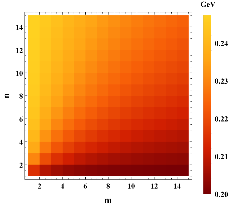
Figure 2: Plot of the energy distribution $|E|$ as a function of the quantum numbers $n$ and $m$, with $q=1$, $M=0.14$ GeV, $k_{z}=0.14$ GeV, $\sigma=1$, $\Lambda=0.80$ and $\alpha_{1}=0.30$ GeV (expressed in natural units).

4.2 Quadratic interaction

Considering $f(r)=\frac{\alpha_{2}r}{2}$, where $\alpha_{2}$ is a constant, this particular form of $f(r)$ leads to $A_{\varphi}=\alpha_{2}H_{0}r^{2}/2$ (quadratic interaction). The choice of the functional form of the four-vector potential was made based on the magnetic field produced by it, which is expected to be a constant magnetic field $\vec{B}=\alpha_{2}\hat{z}$, as indicated in reference durrer2007cosmic . In this scenario, the equation (45) becomes

$$\left[-\frac{d^{2}}{dr^{2}}+\lambda^{2}r^{2}+\frac{\left(m_{\Lambda}^{2}-\frac{1}{4}\right)}{r^{2}}-K^{2}\right]\phi_{1}=0\,,$$ (62)

where $\lambda=q|\alpha_{2}|/2$ and

$$K=\sqrt{E^{2}-M^{2}-k_{z}^{2}+qm_{\Lambda}\alpha_{2}}\,.$$ (63)

Equation (62) defines the relativistic motion of charged scalar bosons interacting with a quadratic vector potential in the context of a Bonnor-Melvin-$\Lambda$ universe. With $\phi_{1}(0)=0$ and $\int_{0}^{\infty}|\phi_{1}|^{2}dr<\infty$, the solution for (62) with $K$ and $\lambda$ real exactly corresponds to the well-known solution of the time-independent radial Schrödinger equation for a harmonic oscillator in two dimensions. Note that the condition $K\in\mathbb{R}$ implies that $|E|>\epsilon$, where

$$\epsilon=\sqrt{M^{2}+k_{z}^{2}-qm_{\Lambda}\alpha_{2}}\,,$$ (64)

for $M^{2}+k_{z}^{2}-qm_{\Lambda}\alpha_{2}\geqslant 0$, and for all $E$ if $M^{2}+k_{z}^{2}-qm_{\Lambda}\alpha_{2}<0$. In this scenario, we only find bound-state solutions.

4.2.1 Bound states

Considering the solution for all $r$ in the form

$$\phi_{1}(r)=r^{|m_{\Lambda}|+\frac{1}{2}}e^{-\lambda r^{2}/2}g(r)\,,$$ (65)

and, along with the definition of a new variable and parameters:

$$\rho = \lambda r^{2}\,,$$ (66)

$$a = \frac{1}{2}\left(|m_{\Lambda}|+1-\frac{K^{2}}{2\lambda}\right)\,,$$ (67)

$$b = |m_{\Lambda}|+1\,,$$ (68)

we find that $g(\rho)$ satisfies a confluent hypergeometric equation ABRAMOWITZ1965 ,

$$\rho\frac{d^{2}g}{d\rho^{2}}+\left(b-\rho\right)\frac{dg}{d\rho}-ag=0\,.$$ (69)

Owing to the condition $\phi_{1}(0)=0$, the regular solution at the origin is given by

$$g(\rho)\propto M\left(a,b,\rho\right)\,.$$ (70)

The asymptotic behavior of Kummer’s function is dictated by ABRAMOWITZ1965

$$M\left(a,b,\rho\right)\simeq\frac{\Gamma(b)}{\Gamma(b-a)}e^{-i\pi a}\rho^{-a}+\frac{\Gamma(b)}{\Gamma(a)}e^{\rho}\rho^{a-b}\,.$$ (71)

It is true that the presence of term $e^{\rho}$ in the asymptotic behavior of $M(a,b,\rho)$ perverts the normalizability of $\phi_{1}(\rho)$. Nevertheless, this trouble can be surpassed by demanding $a=-n$, where $n$ is a nonnegative integer and $b\neq-\tilde{n}$, where $\tilde{n}$ is also a nonnegative integer. In fact, $M(-n,b,\rho)$ with $b>0$ is proportional to the generalized Laguerre polynomial $L_{n}^{(b-1)}(\rho)$, a polynomial of degree $n$ with $n$ distinct positive zeros in the range $[0,\infty)$. Therefore, the solution for all $r$ can be written as

$$\phi_{1}(r)=N_{n}r^{|m_{\Lambda}|+\frac{1}{2}}e^{-\lambda r^{2}/2}L^{(|m_{\Lambda}|)}_{n}(\lambda r^{2})\,,$$ (72)

where $N_{n}$ is a normalization constant. The charge density $J^{0}$ (38) implies that $\phi_{1}$ must be normalized as

$$\frac{|E|}{M}\int_{0}^{\infty}dr|\phi_{1}|^{2}=1\,,$$ (73)

so that, the normalization constant can be expressed as

$$N_{n}=\sqrt{\frac{2M\lambda^{|m_{\Lambda}|+1}\Gamma\left(n+1\right)}{|E|\Gamma\left(|m_{\Lambda}|+n+1\right)}}\,,$$ (74)

with $|E|\neq 0$. Furthermore, the requirement $a=-n$ (quantization condition) implies into

$$E=\pm\sqrt{M^{2}+k_{z}^{2}+q|\alpha_{2}|\left(2n+|m_{\Lambda}|-m_{\Lambda}\mathrm{sgn}(\alpha_{2})+1\right)}\,,$$ (75)

where $\mathrm{sgn}(x)$ is the sign function. From (75), we can see that Landau levels (energy independent of $m$) might occur if only if $m_{\Lambda}\alpha_{2}>0$. Note that the energy spectrum

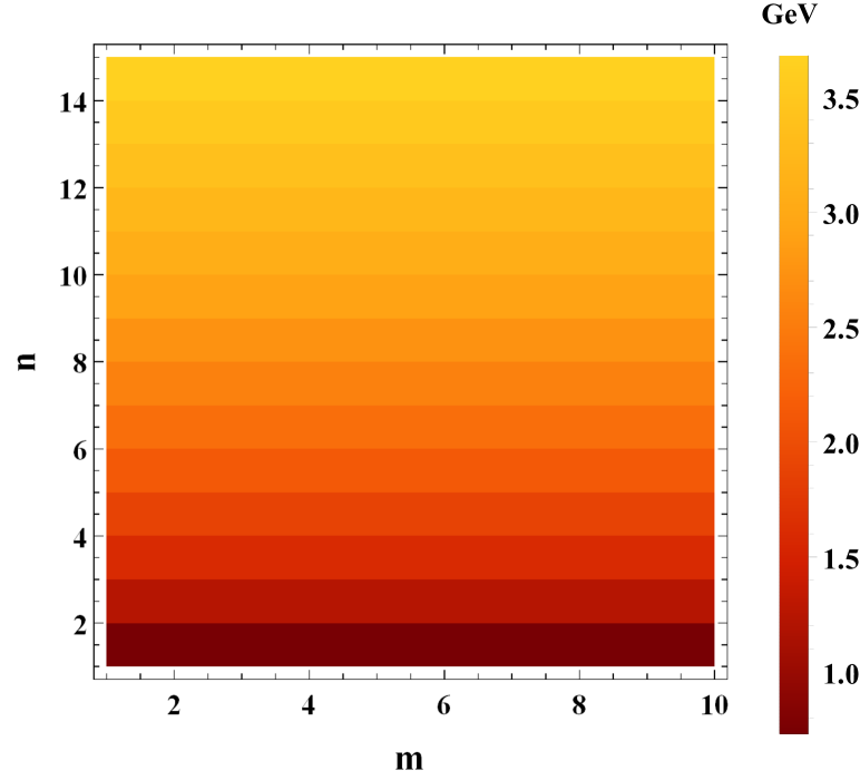
Figure 3: Plot of the energy distribution $|E|$ as a function of the quantum numbers $n$ and $m$, with $q=1$, $M=0.14$ GeV, $k_{z}=0.14$ GeV, $\sigma=1$, $\Lambda=0.80$ and $\alpha_{2}=0.50$ GeV (expressed in natural units).

is composed of particle energy (positive energy) and antiparticle energy (negative energy) and it is symmetrical about $E=0$. As in the previous scenario, we can conclude that this scenario does not distinguish particles from antiparticles. In Fig. 3 displays the energy distribution $|E|$ for bound states as a function of the quantum numbers $n$ and $m$, with $q=1$, $M=0.14$ GeV, $k_{z}=0.14$ GeV, $\sigma=1$, $\Lambda=0.80$ and $\alpha_{2}=0.50$ GeV (expressed in natural units). Here, the cosmological constant, specifically the product $\sqrt{2\Lambda}\sigma$, affects the minimum of the effective potential well, promoting the emergence of more energetic bound states when $\sqrt{2\Lambda}\sigma$ decreases, and vice versa. In this case, we observe the emergence of traditional Landau levels distributed in horizontal bars of varying intensities. Such a characteristic can be explained by the positivity of $\alpha_{2}$ (as per experimental data), which implies that $m$ must also be

positive in order to satisfy the condition $m_{\Lambda}\alpha_{2}>0$. Furthermore, in contrast to the linear case, the absence of an upper energy threshold in this scenario is attributed to the fully confining nature of the effective potential (62).

5 Conclusions

In conclusion, this study was motivated by previous research and aimed to explore the quantum dynamics of a charged scalar boson within the framework of the DKP formalism while immersed in a Bonnor-Melvin-$\Lambda$ universe. The investigation focused on the scalar sector of the DKP equation, yielding the equation of motion for a arbitrary vector potential. Due to the inherent complexity of the equation of motion, we were compelled to employ the limit $\Lambda\ll 1$ to obtain exact solutions. We considered two distinct scenarios for the vector potential: a linear potential and a quadratic potential. In both cases, the problem was transformed into a Schrödinger-like equation for the first component of the DKP spinor. This resulted in Coulomb-like and harmonic oscillator potentials for the linear and quadratic vector potentials, respectively. The remaining components were expressed in a straightforward manner in terms of the first one. For the linear vector potential, the bound-state solutions were determined by identifying the poles of the $S$-matrix. It was observed that the cosmological constant acts as a control parameter, accelerating the accumulation of states at higher energy levels as $\Lambda$ increases, and vice versa. This observation aligns with the findings presented in Fig. 1, which show an increase in the concentration of poles as $\sqrt{2\Lambda}\sigma$ increases. Additionally, it was also observed that the parameters of the problem must satisfy the restriction $m_{\Lambda}\alpha_{1}>0$. In this context, we obtained a symmetric energy spectrum that includes both positive and negative energies, implying an indistinguishability between particles and antiparticles. On the other hand, for the quadratic vector potential, the equation of motion and bound-state solutions were derived from a confluent hypergeometric differential equation. In this scenario, it was observed that the product $\sqrt{2\Lambda}\sigma$ affects the minimum of the effective potential well, promoting the emergence of more energetic bound states when this term decreases, and vice versa. Furthermore, we note that the energy expression is similar to the spectrum shown in the Landau quantization, if only if the restriction on the problem parameters $m_{\Lambda}\alpha_{2}>0$ is satisfied. It is worth highlighting that the energy expression for the bound states, despite its structure, also shows symmetry with respect to $E=0$, as in the previous scenario. Also, we found the normalized solutions for both scenarios expressed in terms of the generalized Laguerre polynomials. The findings in this article suggest that the cosmological constant plays a crucial role in the emergence of bound states and energy quantization.

- (1) G. Petiau, Published in Acad. Roy. de Belg., Classe Sci., Mem in 8o 16, 2 (1936)
- (2) N. Kemmer, Proc. R. Soc. Lond. A 166, 127 (1938). DOI 10.1098/rspa.1938.0084.
- (3) R.J. Duffin, Phys. Rev. 54, 1114 (1938). DOI 10.1103/PhysRev.54.1114.
- (4) N. Kemmer, Proc. R. Soc. Lond. A 173, 91 (1939). DOI 10.1098/rspa.1939.0131.
- (5) M. Nowakowski, Phys. Lett. A 244, 329 (1998). DOI http://dx.doi.org/10.1016/S0375-9601(98)00365-X.
- (6) J.T. Lunardi, B.M. Pimentel, R.G. Teixeira, J.S. Valverde, Phys. Lett. A 268, 165 (2000). DOI http://dx.doi.org/10.1016/S0375-9601(00)00163-8.
- (7) L.B. Castro, A.S. de Castro, Phys. Rev. A 90, 022101 (2014). DOI 10.1103/PhysRevA.90.022101.
- (8) R.F. Guertin, T.L. Wilson, Phys. Rev. D 15, 1518 (1977). DOI 10.1103/PhysRevD.15.1518.
- (9) B. Vijayalakshmi, M. Seetharaman, P.M. Mathews, J. Phys. A: Math. and Gen. 12, 665 (1979). DOI 10.1088/0305-4470/12/5/015.
- (10) Y. Sucu, N. Unal, Eur. Phys. J. C 44(2), 287 (2005). DOI 10.1140/epjc/s2005-02356-0.
- (11) M. Falek, M. Merad, Int. J. Mod. Phys. A 25(13), 2747 (2010). DOI 10.1142/S0217751X10048329.
- (12) E.E. Kangal, H. Yanar, A. Havare, K. Sogut, Ann. Phys. (N.Y.) 343, 40 (2014). DOI https://doi.org/10.1016/j.aop.2014.01.009.
- (13) M. Hosseinpour, H. Hassanabadi, Eur. Phys. J. Plus 130(11), 236 (2015). DOI 10.1140/epjp/i2015-15236-8.
- (14) L.B. Castro, Eur. Phys. J. C 75(6), 287 (2015). DOI 10.1140/epjc/s10052-015-3507-5.
- (15) L.B. Castro, Eur. Phys. J. C 76(2), 61 (2016). DOI 10.1140/epjc/s10052-016-3904-4.
- (16) H. Hassanabadi, M. Hosseinpour, M. de Montigny, Eur. Phys. J. Plus 132(12), 541 (2017). DOI 10.1140/epjp/i2017-11831-y.
- (17) M. Darroodi, H. Mehraban, S. Hassanabadi, EPL 118(1), 10002 (2017). DOI 10.1209/0295-5075/118/10002.
- (18) M. Hosseinpour, H. Hassanabadi, F.M. Andrade, Eur. Phys. J. C 78(2), 93 (2018). DOI 10.1140/epjc/s10052-018-5574-x.
- (19) H. Hassanabadi, S. Zare, M. de Montigny, Gen. Rel. Grav. 50(8), 104 (2018). DOI 10.1007/s10714-018-2429-6.
- (20) M.A. Hun, N. Candemir, Int. J. Mod. Phys. A 34(10), 1950056 (2019). DOI 10.1142/S0217751X19500568.
- (21) M. Achour, L. Khodja, S. Zaim, Int. J. Mod. Phys. A 34(16), 1950082 (2019). DOI 10.1142/S0217751X19500829.
- (22) S. Zare, H. Hassanabadi, M. de Montigny, Gen. Rel. Grav. 52(3), 25 (2020). DOI 10.1007/s10714-020-02676-0.
- (23) H. Chen, Z.W. Long, Y. Yang, Z.L. Zhao, C.Y. Long, Int. J. Mod. Phys. A 35(20), 2050107 (2020). DOI 10.1142/S0217751X20501079.
- (24) Y. Yang, Z.W. Long, H. Chen, Z.L. Zhao, C.Y. Long, Mod. Phys. Lett. A 36(09), 2150059 (2021). DOI 10.1142/S0217732321500590.
- (25) Y. Yang, H. Hassanabadi, H. Chen, Z.W. Long, Int. J. Mod. Phys. E 30(06), 2150050 (2021). DOI 10.1142/S0218301321500506.
- (26) R.R. Cuzinatto, M. de Montigny, P.J. Pompeia, Class. Quant. Grav. 39(7), 075007 (2022). DOI 10.1088/1361-6382/ac51bc.
- (27) N. Candemir, F. Ahmed, Phys. Scr. 98(6), 065224 (2023). DOI 10.1088/1402-4896/acd669.
- (28) N. Candemir, F. Ahmed, Few-Body Syst. 64(2), 13 (2023). DOI 10.1007/s00601-023-01795-z.
- (29) W.B. Bonnor, Proc. Phys. Soc. A 67(3), 225 (1954). DOI 10.1088/0370-1298/67/3/305.
- (30) M. Melvin, Phys. Lett. 8(1), 65 (1964). DOI https://doi.org/10.1016/0031-9163(64)90801-7.
- (31) T.I. Gutsunaev, V.S. Manko, Phys. Lett. A 123(5), 215 (1987). DOI https://doi.org/10.1016/0375-9601(87)90063-6.
- (32) T.I. Gutsunaev, V.S. Manko, Phys. Lett. A 132(2), 85 (1988). DOI https://doi.org/10.1016/0375-9601(88)90257-5.
- (33) L.C.N. Santos, C.C. Barros, Eur. Phys. J. C 76(10), 560 (2016). DOI 10.1140/epjc/s10052-016-4409-x.
- (34) M.A. Dariescu, C. Dariescu, AdHEP 2018, 1953586 (2018). DOI 10.1155/2018/1953586.
- (35) M. Žofka, Phys. Rev. D 99, 044058 (2019). DOI 10.1103/PhysRevD.99.044058.
- (36) L.G. Barbosa, C.C.B. Jr. Scalar bosons in bonnor-melvin- universe: Exact solution, landau levels and coulomb-like potential (2023)
- (37) J.T. Lunardi, B.M. Pimentel, R.G. Teixeira, Gen. Rel. Grav. 34, 491 (2002). DOI 10.1023/A:1015540708007.
- (38) R. Casana, J.T. Lunardi, B.M. Pimentel, R.G. Teixeira, Gen. Rel. Grav. 34, 1941 (2002). DOI 10.1023/A:1020732611995.
- (39) R. R. S. Oliveira, Gen. Relativ. Gravit. 52(9), 88 (2020). DOI 10.1007/s10714-020-02743-6.
- (40) J. A. Huamaní, A. G. Jirón Vicente, A. E. Obispo, R.C. Montero and L.B. Castro, Ann. Phys. (Berlin) 534(11), 2200237 (2022). DOI 10.1002/andp.202200237
- (41) C.C. Soares, A. E. Obispo, A. G. Jirón Vicente and L. B. Castro, Ann. Phys. (Berlin) 535(5), 2200258 (2023). DOI 10.1002/andp.202200258
- (42) Y. Nedjadi, R.C. Barrett, J. Phys. G: Nucl. and Part. Phys. 19, 87 (1993). DOI 10.1088/0954-3899/19/1/006.
- (43) C. Dariescu, M.A. Dariescu, C. Stelea, Adv. High Energy Phys. 2021, 1-10 (2021). DOI 10.1155/2021/5512735.
- (44) H.S. Vieira, V.B. Bezerra, C.R. Muniz, Ann. Phys. 350, 14-28 (2014). DOI 10.1016/j.aop.2014.07.011.
- (45) A.O. Barut, I.H. Duru, Phys. Rev. D 36, 3705 (1987). DOI 10.1103/PhysRevD.36.3705.
- (46) J. Veselỳ, M. Žofka, Phys. Rev. D 103, 024048 (2021). DOI 10.1103/PhysRevD.103.024048.
- (47) J. Veselỳ, Univerzita Karlova, Matematicko-fyzikální fakulta, 2022.
- (48) B. Bellazzini, C. Csáki, J. Hubisz, J. Serra, J. Terning, Eur. Phys. J. C 74(3), 2790 (2014). DOI 10.1140/epjc/s10052-014-2790-x.
- (49) A. Arvanitaki, S. Dimopoulos, V. Gorbenko, J. Huang, K. Van Tilburg, JHEP 2017(5), 71 (2017). DOI 10.1007/JHEP05(2017)071.
- (50) R. Bousso, Gen. Rel. Grav. 40(2), 607 (2008). DOI 10.1007/s10714-007-0557-5.
- (51) M. Demirtas, M. Kim, L. McAllister, J. Moritz, A. Rios-Tascon, Phys. Rev. Lett. 128, 011602 (2022). DOI 10.1103/PhysRevLett.128.011602.
- (52) D.D. Sokolov, A.A. Starobinskii, Sov. Phys Dokl. 22, 312 (1977).
- (53) J.P. Vallée, New Astron. Rev. 48, 763-841 (2004). DOI 10.1016/j.newar.2004.03.017.
- (54) J.B. Seaborn, Hypergeometric Functions and Their Applications (Springer- Verlag, New York, 1991).
- (55) S.N.M. Ruijsenaars, Ann. Phys. (N.Y.) 146(1), 1 (1983). DOI 10.1016/0003-4916(83)90051-9.
- (56) H. Liu, X. Wang, L. Yu, M. Huang, Phys. Rev. D 97, 076008 (2018). DOI 10.1103/PhysRevD.97.076008.
- (57) L.B. Castro, L.P. Oliveira, M.G. Garcia, A.S. Castro, EPJC 77, 1-8 (2017). DOI 10.1140/epjc/s10052-017-4881-y.
- (58) F.A.C. Neto, F.M. Da Silva, L.C.N. Santos, L.B. Castro, Eur. Phys. J. Plus, 135, 1-11 (2020). DOI 10.1140/epjp/s13360-019-00062-7.
- (59) M. Abramowitz, I.A. Stegun, Handbook of Mathematical Functions (Dover, Toronto, 1965).
- (60) R. Durrer, New Astron. Rev. 51, 275-280 (2007). DOI 10.1016/j.newar.2006.11.057.