A geometric formulation to measure global and genuine entanglement in three-qubit systems

Abstract

We introduce a purely geometric formulation for two different measures addressed to quantify the entanglement between different parts of a tripartite qubit system. Our approach considers the entanglement–polytope defined by the smallest eigenvalues of the reduced density matrices of the qubit-components. The measures identify global and genuine entanglement, and are respectively associated with the projection and rejection of a given point of the polytope on the corresponding biseparable segments. Solving the so called ‘inverse problem’, we also discuss a way to force the system to behave in a particular form, which opens the possibility of controlling and manipulating entanglement for practical purposes.

1 Introduction

Entanglement is the most interesting nonclassical correlation of multipartite quantum systems. It represents an important resource in quantum computing, quantum information processing and quantum teleportation [1, 2, 3]. However, the characterization and quantification of multipartite entanglement is still an open question [4, 5]. Even in the three-qubit system case it has been pointed out that different forms of entanglement may be present [6, 7, 8, 9]. This can be seen from the fact that there is no unified notion of a maximally entangled state. In fact, considering the most widely used measures [10], different requirements comprise different characteristics of the nonlocal properties that a given system must satisfy to exhibit maximal entanglement.

In this sense, entanglement measures based on the geometry of the state space or the appropriate projective space are of particular interest. For example, the geometric measure of entanglement (GME) evaluates the distance from a target state to its closest separable state in a given Hilbert space [11, 12]. Although its immediate geometric interpretation, the GME demands a non-trivial optimization so it becomes a nondeterministic polynomial (NP) problem [13]. Indeed, the amount of information that must be processed suggests that sooner or later it will be inevitable to resort to numerical methods [12]. Other examples includes the entanglement of minimum bipartite entropy [14], which quantifies the distance of a given state with its nearest state with no three-way entanglement, and robustness [15].

With respect to the geometry of projective spaces, for permutation invariant states, the Majorana representation leads to the identification of maximal symmetric $n$-qubit states [16, 17]; it has also been reported an entanglement measure associated with the barycenter of the Majorana constellation [16]. More recently, the triangle whose edges correspond to the squared bipartite concurrence of a three-qubit system has been considered as a useful tool to quantify entanglement [18]. It has been shown that the genuinely multipartite concurrence defined in [19] is exactly the square root of the shortest edge length of such a triangle, and that its perimeter is nothing else than the global entanglement measure considered in [20, 21]. Remarkably, the concurrence triangle area, computed through the Heron’s formula, is associated with a genuine entangled measure referred to as the concurrence fill [18].

Of particular interest, the three qubit entanglement–polytope permits the introduction of some criteria for the characterization and detection of entanglement [22, 23, 28, 29, 30, 24, 25, 31, 26, 27]. To deepen the understanding of entanglement classification, the relationship between the entanglement types introduced in [7, 8] and some subsets of the polytope [24, 25] has been analyzed. In this context, a relationship between the linear entropy of entanglement [20, 21] and the Euclidean distance to one of the vertices of the polytope has been observed [23, 32]. However, most of the characterization of the entanglement–polytope studied so far has been done qualitatively.

In this work, we study the entanglement between different parts of a tripartite qubit system from a purely geometric perspective. Our approach considers the entanglement polytope defined by the smallest eigenvalues of the reduced density matrices. We introduce a mapping from the state space to the polytope that leads to identifying some relationships between tripartite quantum states and points with clear geometric interpretation in the polytope. Then, fully separable, bi-separable and non-separable states are associated with concrete subsets (vertices, edges, facets, etc) of the polytope, providing a geometric identification of entanglement.

The most striking feature of our approach is to find that the projection and rejection of a given point of the polytope into the corresponding biseparable subsets yields a way to quantify entanglement. The former identifies global entanglement and the latter indicates genuine entanglement.

As a byproduct, we look for a way to force the system to behave in a particular form. The cornerstone is provided by solutions to the inverse problem: given a point on the polytope in a region that characterizes very specific entanglement properties, the quantum state that satisfies such a profile must be found. We show that this approach offers interesting challenges and a much broader perspective on nonclassical correlations since it opens the possibility of controlling and manipulating entanglement for practical purposes.

In Section 2 we review the convex structure of the three-qubit polytope and some entanglement properties are characterized qualitatively. A quantitative description of the three-qubit entanglement is provided in Section 3, where we propose two distance-based entanglement measures, one quantifying the global entanglement and the other characterizing the three-qubit genuine entanglement. Section 4 is addressed to solve the inverse problem. Some conclusions are given in Section 5.

2 Qualitative characterization of entanglement

Let $\mathcal{H}=\mathcal{H}_{2}\otimes\mathcal{H}_{2}\otimes\mathcal{H}_{2}$ be the Hilbert space of a three-qubit system, with $\mathcal{H}_{2}$ the two-dimensional space of states for a single qubit. Given a pure state $|\psi\rangle\in\mathcal{H}$, written in the standard form [7, 8],

$$|\psi\rangle=b_{0}|000\rangle+b_{1}e^{i\theta}|100\rangle+b_{2}|101\rangle+b_{3}|110\rangle+b_{4}|111\rangle,\quad b_{\ell}\geq 0,\quad\sum_{\ell=0}^{4}b_{\ell}^{2}=1,$$ (1)

with $0\leq\theta\leq\pi$, we will pay attention to the vector $\vec{\lambda}_{\psi}=\left(\lambda_{1},\lambda_{2},\lambda_{3}\right)^{T}$, where $\lambda_{k}$ is the smallest eigenvalue of the density matrix $\rho_{k}$ associated to the $k$th qubit.

Looping through all allowed values of $b_{\ell}$ and $\theta$ in (1), vector $\vec{\lambda}_{\psi}$ localizes the points of a convex polytope $\mathcal{P}\subset\mathbb{R}^{3}$ that encodes the degree of entanglement between the different parts of a tripartite qubit system [24, 23, 25]. Therefore, we consider the mapping

$$\Lambda:$$

,

(2)

together with the inequalities [26]:

$$\lambda_{i}\leq\lambda_{j}+\lambda_{k},\quad 0\leq\lambda_{i}\leq\tfrac{1}{2},\quad i,j,k=1,2,3.$$ (3)

Figure 1 shows the entanglement–polytope $\mathcal{P}$ that we are dealing with. It is a body that resembles two tetrahedra, joined at their base, embedded in a cube with edges of length equal to $\nicefrac{{1}}{{2}}$, located at the first octant of $\mathbb{R}^{3}$. To be concrete, $\mathcal{P}$ is defined by the convex combination of its vertices

$$\begin{array}[]{ccc}\vec{S}=(0,0,0)^{T},\quad\vec{B}_{1}=\left(0,\tfrac{1}{2},\tfrac{1}{2}\right)^{T},\quad\vec{B}_{2}=\left(\tfrac{1}{2},0,\tfrac{1}{2}\right)^{T},\\[8.00002pt] \vec{B}_{3}=\left(\tfrac{1}{2},\tfrac{1}{2},0\right)^{T},\quad\vec{G}=\left(\tfrac{1}{2},\tfrac{1}{2},\tfrac{1}{2}\right)^{T}.\end{array}$$ (4)

Characterizing multipartite entanglement in terms of entanglement–polytopes is very useful since only one-particle information is required [22, 23], see also [24] and [27]. Remarkably, this picture finds immediate application in detection processes of entanglement since its predictions do not require the measurement of correlations between the parts. For example, the experimental detection of entanglement–polytopes for three- and four-qubit genuine entanglement occurring in quantum optics has been reported in [28, 29], a fact that shows the practical usefulness of the method.

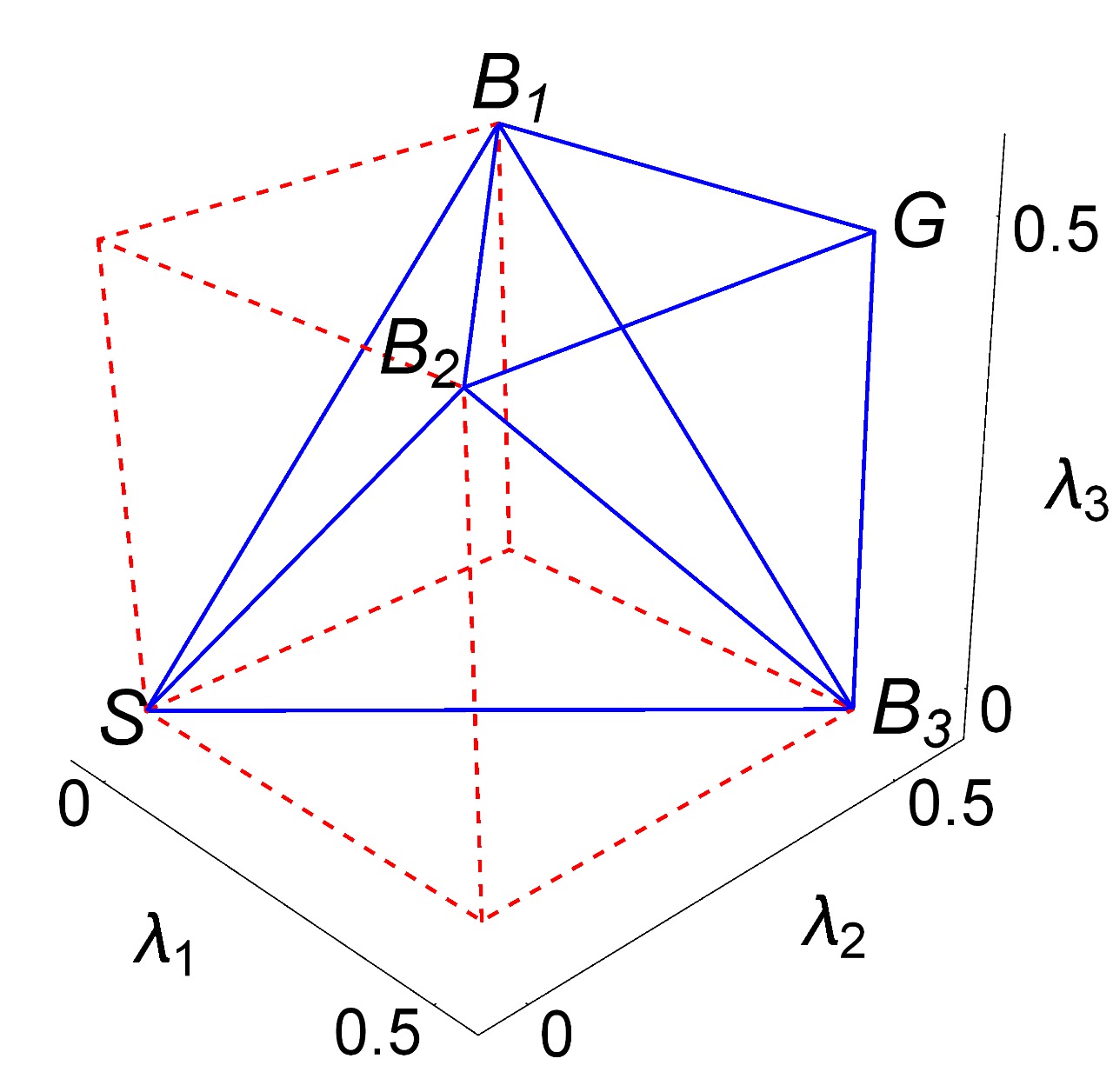
Figure 1: Entanglement–polytope $\mathcal{P}\subset\mathbb{R}^{3}$ associated with the three-qubit states (1). It is a body that resembles two tetrahedra, joined at their base, embedded in a cube with edges of length equal to $\nicefrac{{1}}{{2}}$. The parameter $\lambda_{k}$ (defining the corresponding axis) is the smallest eigenvalue of the density matrix associated with the $k$th qubit. Vertex $\vec{S}$ represents the entire set of fully separable states while $\vec{G}$ corresponds to the Greenberger–Horne–Zeilinger state. The vertices $\vec{B}_{i}$ correspond to bi-separable states $|\phi_{i}\rangle|\phi_{jk}\rangle$, with $|\phi_{i}\rangle$ the state of the $i$th qubit and $|\phi_{jk}\rangle$ a Bell state in the bipartition $i-jk$.

In general, depending on the number of parameters $b_{\ell}\neq 0$ that characterize the linear combination (1), there is a classification of entangled states [7, 8] that is summarized in Table 1. Next, based on the results reported in [24], we show that this classification results in the identification of concrete convex subsets of $\mathcal{P}$ under the mapping $\Lambda$.

Type	Basis product states	Subset $\subseteq\mathcal{P}$
1	$\{|000\rangle\}$	$\vec{S}$
2a-1	$\{|101\rangle,|110\rangle\}$	$\overline{SB_{1}}$
2a-2	$\{|000\rangle,|101\rangle\}$	$\overline{SB_{2}}$
2a-3	$\{|000\rangle,|110\rangle\}$	$\overline{SB_{3}}$
2b	$\{|000\rangle,|111\rangle\}$	$\overline{SG}$
3a	$\{|000\rangle,|101\rangle,|110\rangle\}$	Facets of $SB_{1}B_{2}B_{3}$
3b-1	$\{|000\rangle,|100\rangle,|111\rangle\}$	$SB_{1}G$
3b-2	$\{|000\rangle,|101\rangle,|111\rangle\}$	$SB_{2}G$
3b-3	$\{|000\rangle,|110\rangle,|111\rangle\}$	$SB_{3}G$
4a	$\{|000\rangle,|100\rangle,|101\rangle,|110\rangle\}$	$SB_{1}B_{2}B_{3}$
4b-1	$\{|000\rangle,|100\rangle,|110\rangle,|111\rangle\}$	$\subset SB_{1}B_{3}G$
4b-2	$\{|000\rangle,|100\rangle,|101\rangle,|111\rangle\}$	$\subset SB_{1}B_{2}G$
4c	$\{|000\rangle,|101\rangle,|110\rangle,|111\rangle\}$	$SB_{1}B_{2}B_{3}\cup SB_{2}B_{3}G$
4d	$\{|001\rangle,|010\rangle,|100\rangle,|111\rangle\}$	$\mathcal{P}$
5	$\{|000\rangle,|100\rangle,|101\rangle,|110\rangle,|111\rangle\}$	$\mathcal{P}$

Table 1: The number of basis elements of $\mathcal{H}=\mathcal{H}_{2}\otimes\mathcal{H}_{2}\otimes\mathcal{H}_{2}$ that are included in the linear superposition (1) gives rise to a classification of three-qubit states [7, 8]. Some of the representative states generated by such basis elements are associated with specific convex subspaces of the entanglement–polytope $\mathcal{P}\subset\mathbb{R}^{3}$ shown in Figure 1, see [24] and discussion in the main text. The class generated by any base element of $\mathcal{H}$ contains type 1 states; in the table we use $|000\rangle$ as a generic case.

The simplest class, called type 1, refers to superpositions (1) with only one coefficient different from zero. Any state of this type is fully separable, hereafter we write $|\psi_{\operatorname{sep}}\rangle=\ket{\phi_{1}}\ket{\phi_{2}}\ket{\phi_{3}}$, with $|\phi_{i}\rangle\in\mathcal{H}_{2}$. The latter implies that the smallest eigenvalue $\lambda_{k}$ of $\rho_{k}$ is equal to zero for all $i=1,2,3$. Thus, the entire set of vectors $|\psi_{\operatorname{sep}}\rangle$ (represented by $|000\rangle$ in Table 1) is associated with the vertex $\vec{S}\in\mathcal{P}$, which is a 0-dimensional convex set.

Type 2 includes linear superpositions (1) with two coefficients different from zero. We identify two different subclasses, called 2a and 2b.

Type 2a is subdivided into three different categories, called 2a-1, 2a-2 and 2a-3, which refer to the superpositions (1) characterized by the pairs $\{b_{2},b_{3}\}$, $\{b_{0},b_{2}\}$ and $\{b_{0},b_{3}\}$, respectively. These states are bi-separable, written $\ket{\psi_{\operatorname{bi}}}=\ket{\phi_{i}}\ket{\phi_{jk}}$, with $\ket{\phi_{jk}}$ a non-separable state shared by the $j$th and $k$th qubits (the sub labels are cyclic). They correspond to the one-dimensional convex subsets of $\mathcal{P}$ generated by the vertices $\vec{S}$ and $\vec{B}_{i}$. That is, type 2a states are associated with the line-segments (edges) $\overline{SB_{1}}$, $\overline{SB_{2}}$ and $\overline{SB_{3}}$ of $\mathcal{P}$. For instance, if $\ket{\psi_{\operatorname{bi}}}=b_{2}\ket{101}+b_{3}\ket{110}$, then $\vec{\lambda}_{\psi_{\operatorname{bi}}}=(1-2\lambda)\vec{S}+2\lambda\vec{B}_{1}$, where $\lambda=(1-\sqrt{1-4b_{2}^{2}b_{3}^{2}})/2$. Similarly for types 2a-2 and 2a-3. Stellar members of type 2a are the bi-separable states linked to the vertices $\vec{B}_{i}\in\mathcal{P}$, for which $\ket{\phi_{jk}}$ is one of the Bell–basis elements $\sqrt{2}|\Phi^{\pm}\rangle=|00\rangle\pm|11\rangle$, $\sqrt{2}|\Psi^{\pm}\rangle=|01\rangle\pm|10\rangle$.

Type 2b includes superpositions (1) that are characterized by the pair $\{b_{0},b_{4}\}$. These states are associated with the one-dimensional convex subset generated by the extremal points $\vec{S}$ and $\vec{G}$ (the line-segment $\overline{SG}$). Explicitly, $\vec{\lambda}_{\psi_{2b}}=(1-2\lambda)\vec{S}+2\lambda\vec{G}$, where $\lambda=(1-\sqrt{1-4b_{0}^{2}b_{4}^{2}})/2$. The Greenberger–Horne–Zeilinger (GHZ) state

$$|GHZ\rangle=\frac{1}{\sqrt{2}}\left(|000\rangle+|111\rangle\right)$$

corresponds to the extremal point $\vec{G}$.

States of type 3 involve three coefficients different from zero in the linear superposition (1). They are associated with two-dimensional convex subsets of $\mathcal{P}$, as we indicate below.

The type 3a refers to vectors that can be written in the form

$$|\psi_{\rm 3a}\rangle=\sqrt{\gamma}|000\rangle+\sqrt{\alpha}|101\rangle+\sqrt{\beta}|110\rangle,\quad 0\leq\alpha,\beta\leq 1,\quad\gamma=1-\alpha-\beta.$$ (5)

Therefore, the components of $\vec{\lambda}_{\psi_{\rm 3a}}$ are as follows

$$\lambda_{1}=\tfrac{1}{2}-\left|\gamma-\tfrac{1}{2}\right|,\quad\lambda_{2}=\tfrac{1}{2}-\left|\beta-\tfrac{1}{2}\right|,\quad\lambda_{3}=\tfrac{1}{2}-\left|\alpha-\tfrac{1}{2}\right|.$$

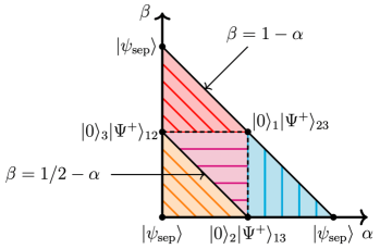
Figure 2: The parameters $\alpha$ and $\beta$ completely define the state $|\psi_{3a}\rangle$ introduced in Eq. (5). The constraints on these parameters give rise to the convex set $\mathcal{M}$, a right triangle with legs of one unit on the plane $\mathbb{R}^{2}$. The extreme points, $(\alpha,\beta)=(0,0)$, $(0,1)$ and $(1,0)$, characterize $|\psi_{3a}\rangle$ as a fully separable state. The middle points, $(\nicefrac{{1}}{{2}},\nicefrac{{1}}{{2}})$, $(\nicefrac{{1}}{{2}},0)$ and $(0,\nicefrac{{1}}{{2}})$, produce the bi-separable states $|0\rangle_{i}|\Psi^{+}\rangle_{jk}$, where $|\Psi^{+}\rangle_{jk}$ stands for the Bell state $|\Psi^{+}\rangle$ shared by the $j$th and $k$th qubits. The convex combinations of extreme and middle points yield four different convex subsets (regions) of $\mathcal{M}$ that permit a classification of entanglement for $|\psi_{3a}\rangle$.

Figure 2 shows the convex set $\mathcal{M}\subset\mathbb{R}^{2}$ that arises from the constraints on the parameters $\alpha$ and $\beta$ in Eq. (5). It is a right triangle with legs of one unit. The extreme points, $(\alpha,\beta)=(0,0)$, $(0,1)$ and $(1,0)$, define fully separable states that are mapped onto the vertex $\vec{S}$ of $\mathcal{P}$. In turn, the middle points, $(\nicefrac{{1}}{{2}},\nicefrac{{1}}{{2}})$, $(\nicefrac{{1}}{{2}},0)$ and $(0,\nicefrac{{1}}{{2}})$, produce the bi-separable states that are mapped onto the vertices $\vec{B}_{i}$ of $\mathcal{P}$. The data shown in Figure 2 is obtained from (5), after the appropriate local unitary transformation. The convex combinations of extreme and middle points yield four different convex subsets (regions) of $\mathcal{M}$ that permit a classification of entanglement for the state $|\psi_{3a}\rangle$.

Region I. The convex set $\alpha\in[\nicefrac{{1}}{{2}},1]$, $\beta\in[0,1-\alpha]$, represented in Figure 2 as the right triangle in blue, yields the parametrization

$$\vec{\lambda}_{\psi_{\rm 3a}}=\kappa_{1}\vec{S}+\kappa_{2}\vec{B}_{1}+\kappa_{3}\vec{B}_{2},$$ (6)

where $\kappa_{1}=2\alpha-1$, $\kappa_{2}=2\beta$, and $\kappa_{3}=1-\kappa_{1}-\kappa_{2}$. Vectors (6) localize the points on the triangle $\triangle_{SB_{1}B_{2}}\in\mathcal{P}$, see Figure 3(a).

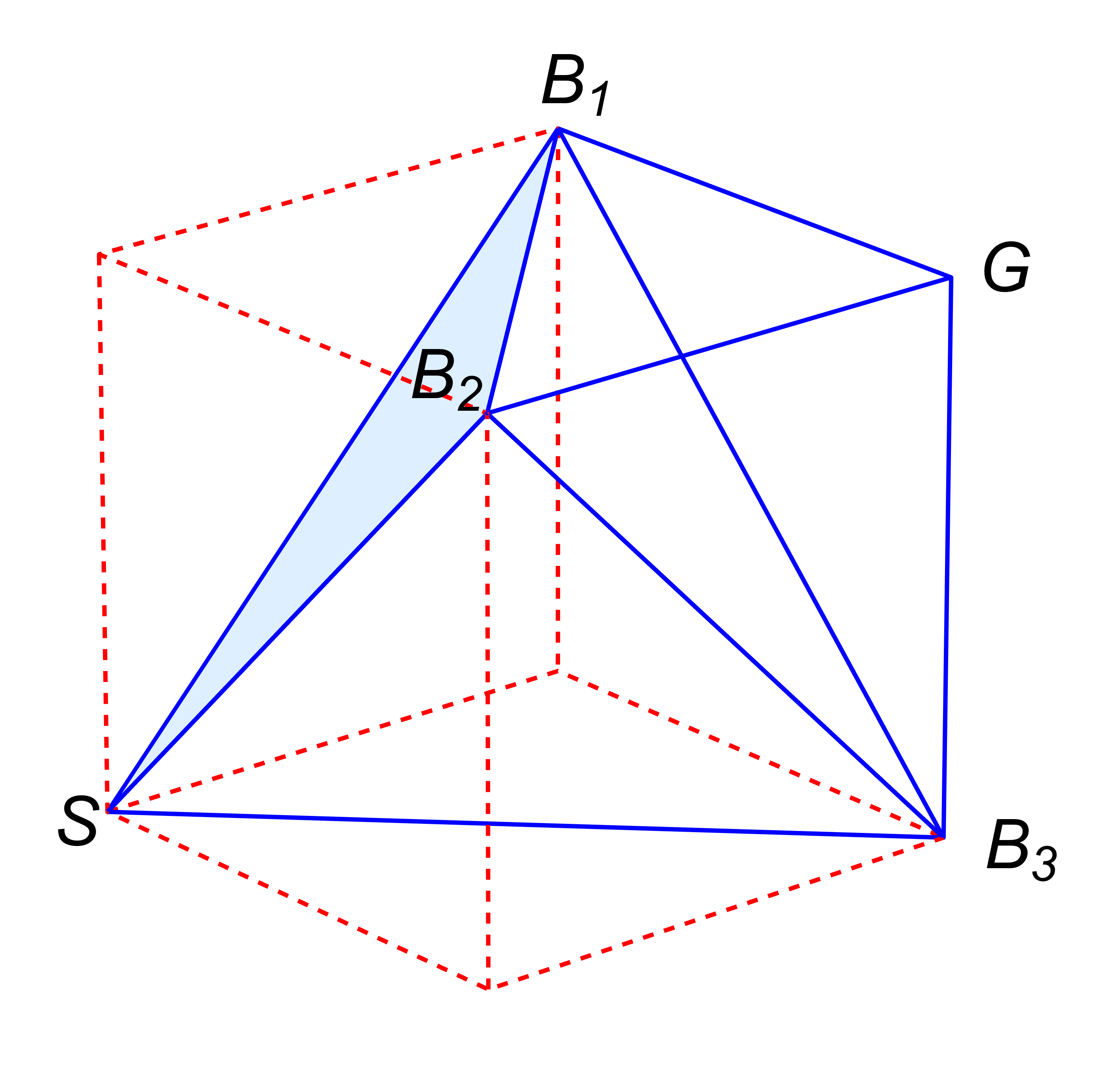
(a) Region I

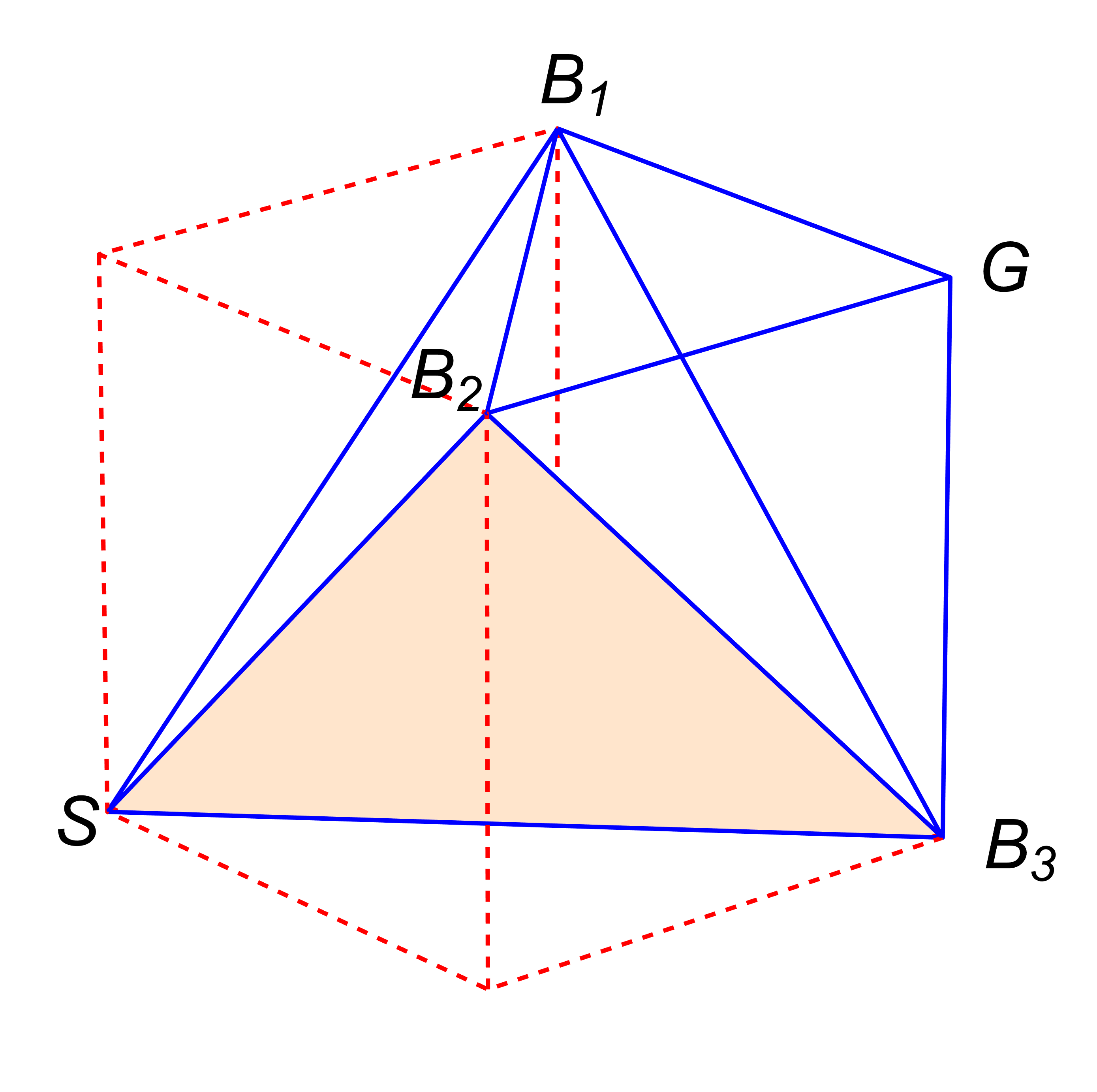
(b) Region II

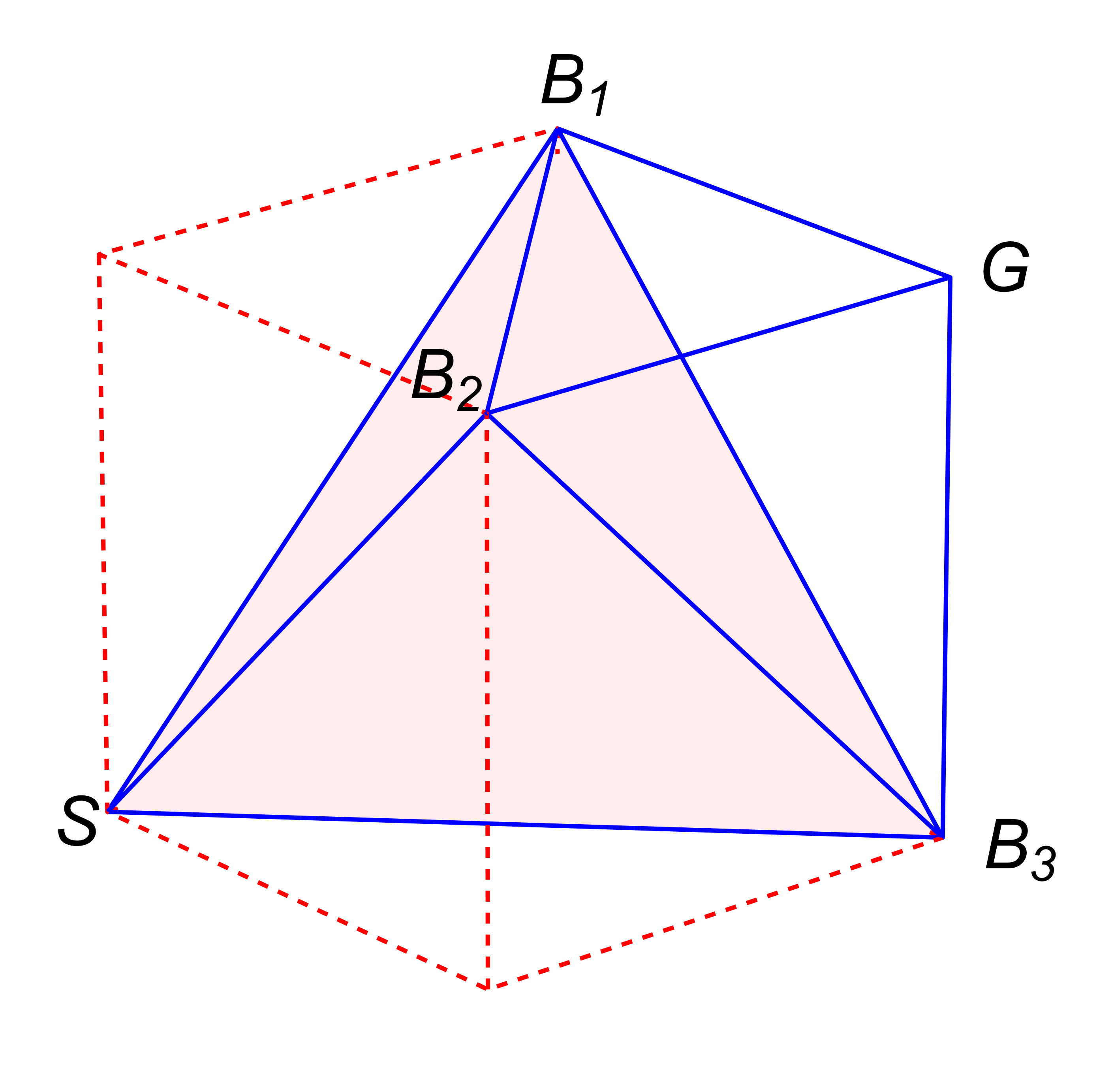
(c) Region III

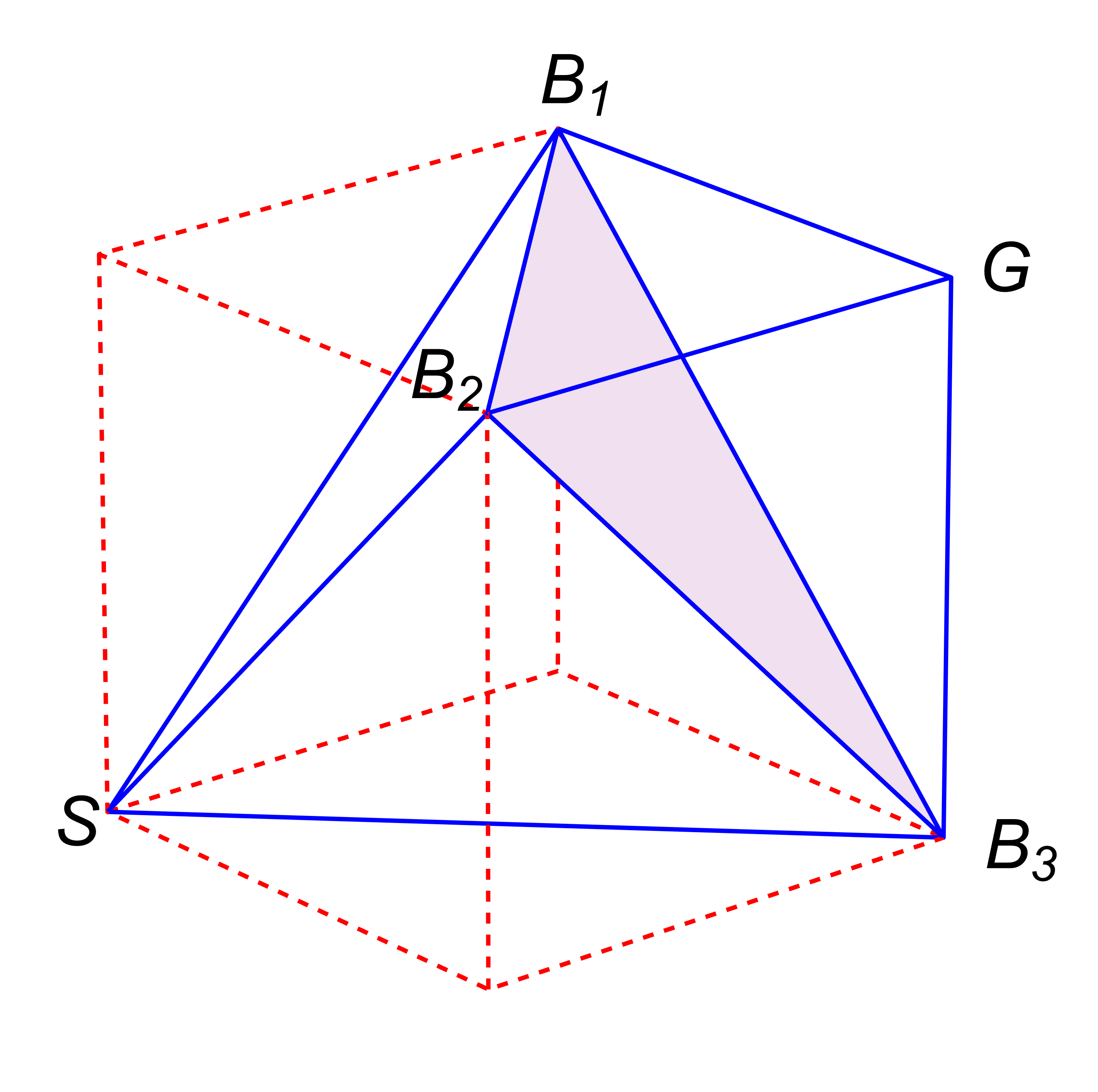
(d) Region IV

Figure 3: The four different regions of the convex set $\mathcal{M}$ illustrated in Figure 2 are associated with the faces of the lower tetrahedron of the polytope $\mathcal{P}$. The color-code corresponds to the colors of the right-triangles in Figure 2.

Region II. The right triangle in orange of Figure 2 corresponds to the convex set $\alpha\in[0,\nicefrac{{1}}{{2}}]$, $\beta\in[0,\nicefrac{{1}}{{2}}-\alpha]$, and gives

$$\vec{\lambda}_{\psi_{\rm 3a}}=\kappa_{1}\vec{S}+\kappa_{2}\vec{B}_{2}+\kappa_{3}\vec{B}_{3},$$ (7)

with $\kappa_{2}=2\alpha$, $\kappa_{3}=2\beta$ and $\kappa_{1}=1-\kappa_{2}-\kappa_{3}$. In this case, the vectors (7) localize the points on the triangle $\triangle_{SB_{2}B_{3}}\in\mathcal{P}$, see Figure 3(b).

Region III. The right triangle in pink of Figure 2 represents the convex set $\alpha\in[0,\nicefrac{{1}}{{2}}]$, $\beta\in[\nicefrac{{1}}{{2}},1-\alpha]$. This yields

$$\vec{\lambda}_{\psi_{\rm 3a}}=\kappa_{1}\vec{S}+\kappa_{2}\vec{B}_{1}+\kappa_{3}\vec{B}_{3},$$ (8)

with $\kappa_{1}=2\alpha-1$, $\kappa_{2}=2\beta$ and $\kappa_{3}=1-\kappa_{1}-\kappa_{2}$. The points on the triangle $\triangle_{SB_{1}B_{3}}\in\mathcal{P}$ of Figure 3(c) are localized by the vectors (8).

Region IV. The right triangle in light-purple of Figure 2 stands for the convex set $\alpha\in[0,\nicefrac{{1}}{{2}}]$, $\beta\in[\nicefrac{{1}}{{2}}-\alpha,\nicefrac{{1}}{{2}}]$. The corresponding vectors

$$\vec{\lambda}_{\psi_{\rm 3a}}=\kappa_{1}\vec{B}_{1}+\kappa_{2}\vec{B}_{2}+\kappa_{3}\vec{B}_{3},$$ (9)

with $\kappa_{2}=1-2\beta$, $\kappa_{3}=1-2\alpha$ and $\kappa_{1}=1-\kappa_{2}-\kappa_{3}$, localize the points on the triangle $\triangle_{B_{1}B_{2}B_{3}}\in\mathcal{P}$ shown in Figure 3(d).

The latter case is of particular relevance. Making $\alpha=\beta=1/3$ we have the state

$$|\psi_{\rm 3a}\rangle=\tfrac{1}{\sqrt{3}}\left(\ket{000}+\ket{101}+\ket{110}\right),$$

which is local unitary equivalent to the well-known W–state,

$$|W\rangle=\tfrac{1}{\sqrt{3}}\left(\ket{001}+\ket{010}+\ket{100}\right).$$ (10)

Explicitly, $|\psi_{\rm 3a}\rangle=\left(\sigma_{x}\otimes\mathds{1}\otimes\mathds{1}\right)|W\rangle$, with $\sigma_{x}$ the $x$–Pauli matrix and $\mathds{1}$ the identity operator in $\mathcal{H}_{2}$. Since the smallest eigenvalues are local unitary invariant [33, 34] both, $|\psi_{\rm 3a}\rangle$ and $|W\rangle$, are mapped onto the same point $\vec{\lambda}_{W}=\left(\nicefrac{{1}}{{3}},\nicefrac{{1}}{{3}},\nicefrac{{1}}{{3}}\right)^{T}\in\mathcal{P}$, which is the geometric center of the triangle $\triangle_{B_{1}B_{2}B_{3}}\subset\mathcal{P}$.

On the other hand, the type 3b includes three different families of vectors, given by the expressions

$$\begin{array}[]{l}|\psi_{\rm 3b-1}\rangle=b_{0}|000\rangle+b_{1}e^{i\theta}|100\rangle+b_{4}|111\rangle,\\[6.88889pt] |\psi_{\rm 3b-2}\rangle=b_{0}|000\rangle+b_{2}|101\rangle+b_{4}|111\rangle,\\[6.88889pt] |\psi_{\rm 3b-3}\rangle=b_{0}|000\rangle+b_{3}|110\rangle+b_{4}|111\rangle.\end{array}$$ (11)

They correspond respectively to the triangles $\triangle_{SB_{1}G}$, $\triangle_{SB_{2}G}$, and $\triangle_{SB_{3}G}$, see Figure 4.

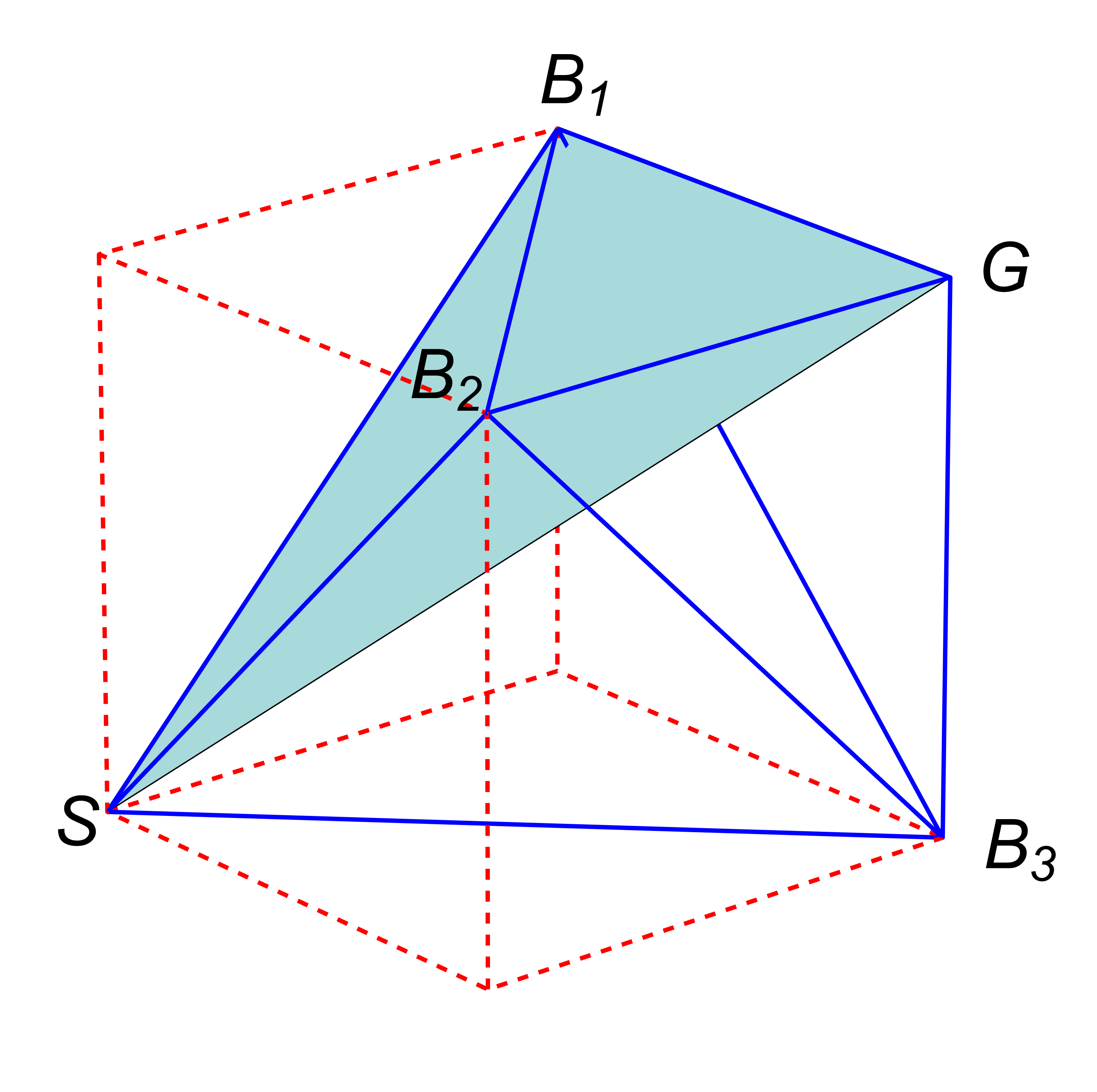
(a) Type 3b-1

(b) Type 3b-2

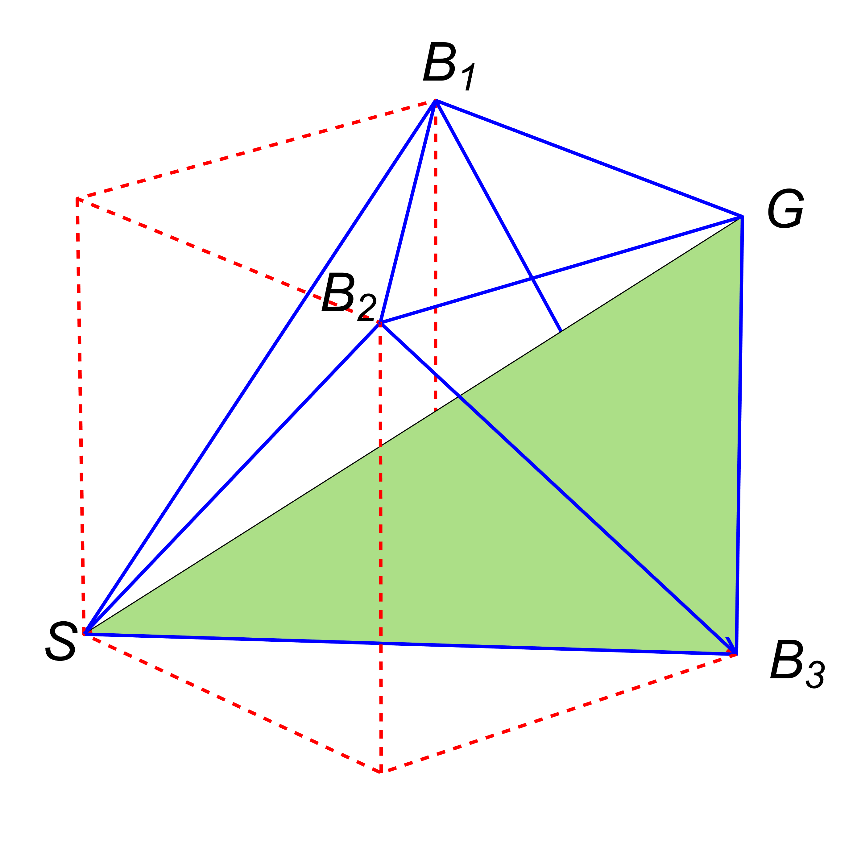
(c) Type 3b-3

Figure 4: The type 3b-$i$ states (11) are associated with the two-dimensional convex subsets that are different from the faces of the tetrahedra that form the polytope $\mathcal{P}$.

The type 4, referring to superpositions (1) that admit four non-zero coefficients, corresponds to three-dimensional convex subsets of $\mathcal{P}$ that are subdivided into four different clases.

Type 4a, with $b_{4}=0$, is restricted to the lower tetrahedron of $\mathcal{P}$, written $SB_{1}B_{2}B_{3}$, where $\lambda_{1}+\lambda_{2}+\lambda_{3}\leq 1$ [24]. The identity in this inequality is saturated by the points on the triangle $\triangle_{B_{1}B_{2}B_{3}}$.

Type 4b is subdivided into two different categories, called b-1 (with $b_{2}=0$) and b-2 (with $b_{3}=0$). They are respectively mapped into a subset of $SB_{1}B_{3}G$ and $SB_{1}B_{2}G$ [25].

For states of type 4c (with $b_{1}=0$), let us consider the linear superposition

$$\ket{\psi_{4c-1}}=\tfrac{1}{\sqrt{2}}\ket{000}+b_{2}\ket{101}+b_{3}\ket{110}+b_{4}\ket{111},$$ (12)

where $b_{2}^{2}+b_{3}^{2}+b_{4}^{2}=\nicefrac{{1}}{{2}}$. In this case, the vector

$$\vec{\lambda}_{\psi_{\rm 4c-1}}=\kappa_{1}\vec{B}_{2}+\kappa_{2}\vec{B}_{3}+\kappa_{3}\vec{G},$$ (13)

with

$$\kappa_{1}=2\sqrt{b_{2}^{2}\left(\tfrac{1}{2}-b_{3}^{2}\right)},\quad\kappa_{2}=2\sqrt{b_{3}^{2}\left(\tfrac{1}{2}-b_{2}^{2}\right)},\quad\kappa_{3}=1-\kappa_{1}-\kappa_{2},$$ (14)

localizes the points on the triangle $\triangle_{B_{2}B_{3}G}$. The appropriate permutations transform (12) into a pair of additional states of type 4c. Namely,

$$\begin{array}[]{ll}\ket{\psi_{4c-2}}=\frac{1}{\sqrt{2}}\ket{000}+b_{2}\ket{110}+b_{3}\ket{011}+b_{4}\ket{111},\\[6.88889pt] \ket{\psi_{4c-3}}=\frac{1}{\sqrt{2}}\ket{000}+b_{2}\ket{011}+b_{3}\ket{101}+b_{4}\ket{111},\end{array}$$ (15)

where $\sum b_{i}=\nicefrac{{1}}{{2}}$. It is immediate to show that these states are mapped into the triangles $\triangle_{B_{1}B_{3}G}$ and $\triangle_{B_{1}B_{2}G}$, respectively. That is, with type 4c-$i$ states, $i=1,2,3$, we cover the three faces of the upper tetrahedron in $\mathcal{P}$, see Figure 5.

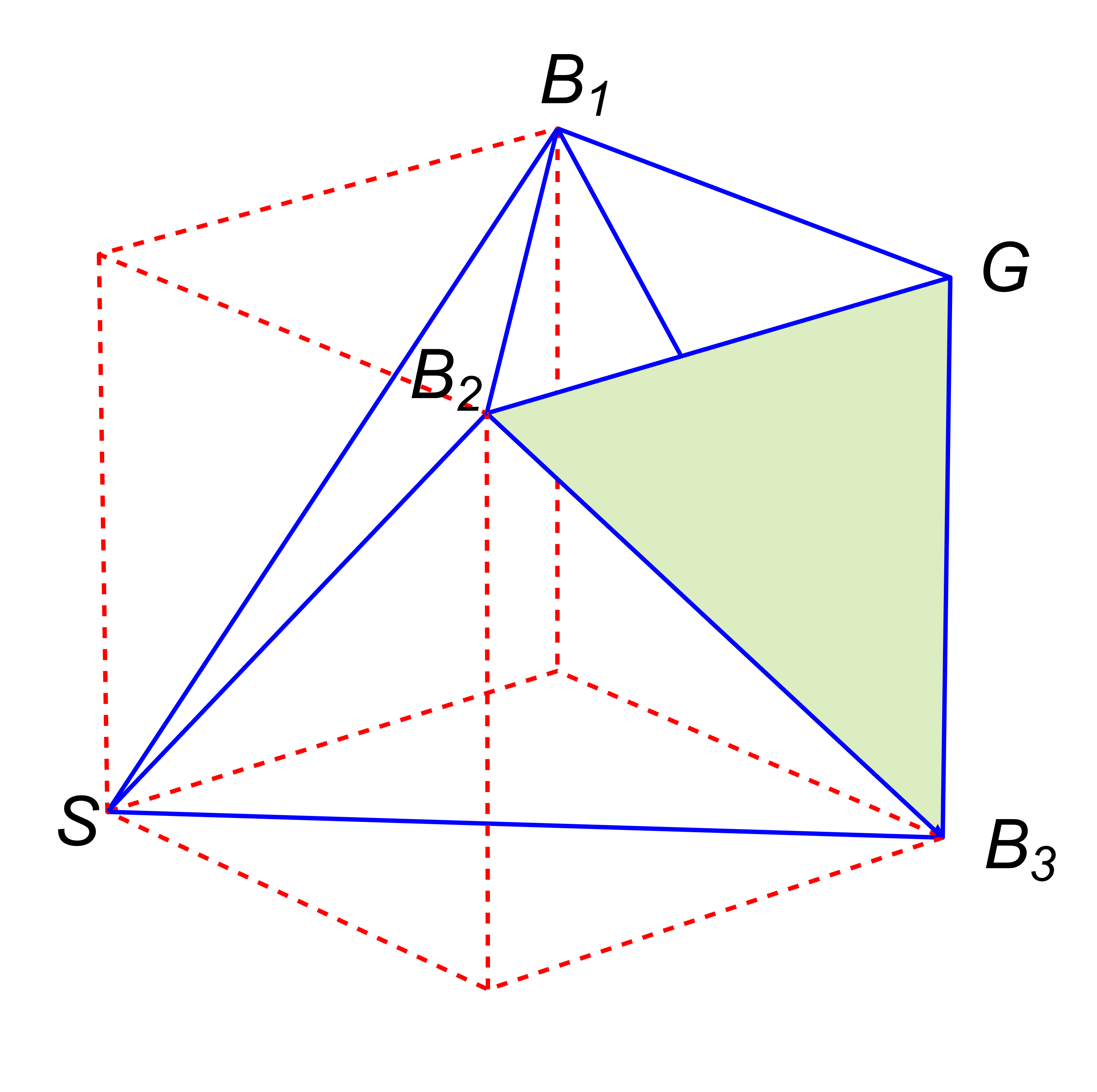
(a) Type 4c-1

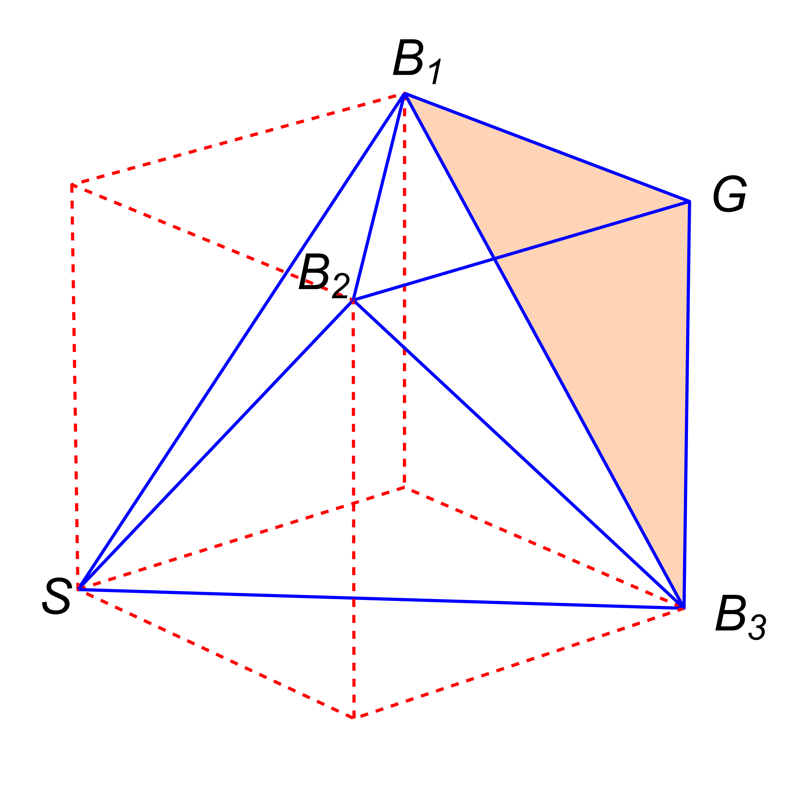
(b) Type 4c-2

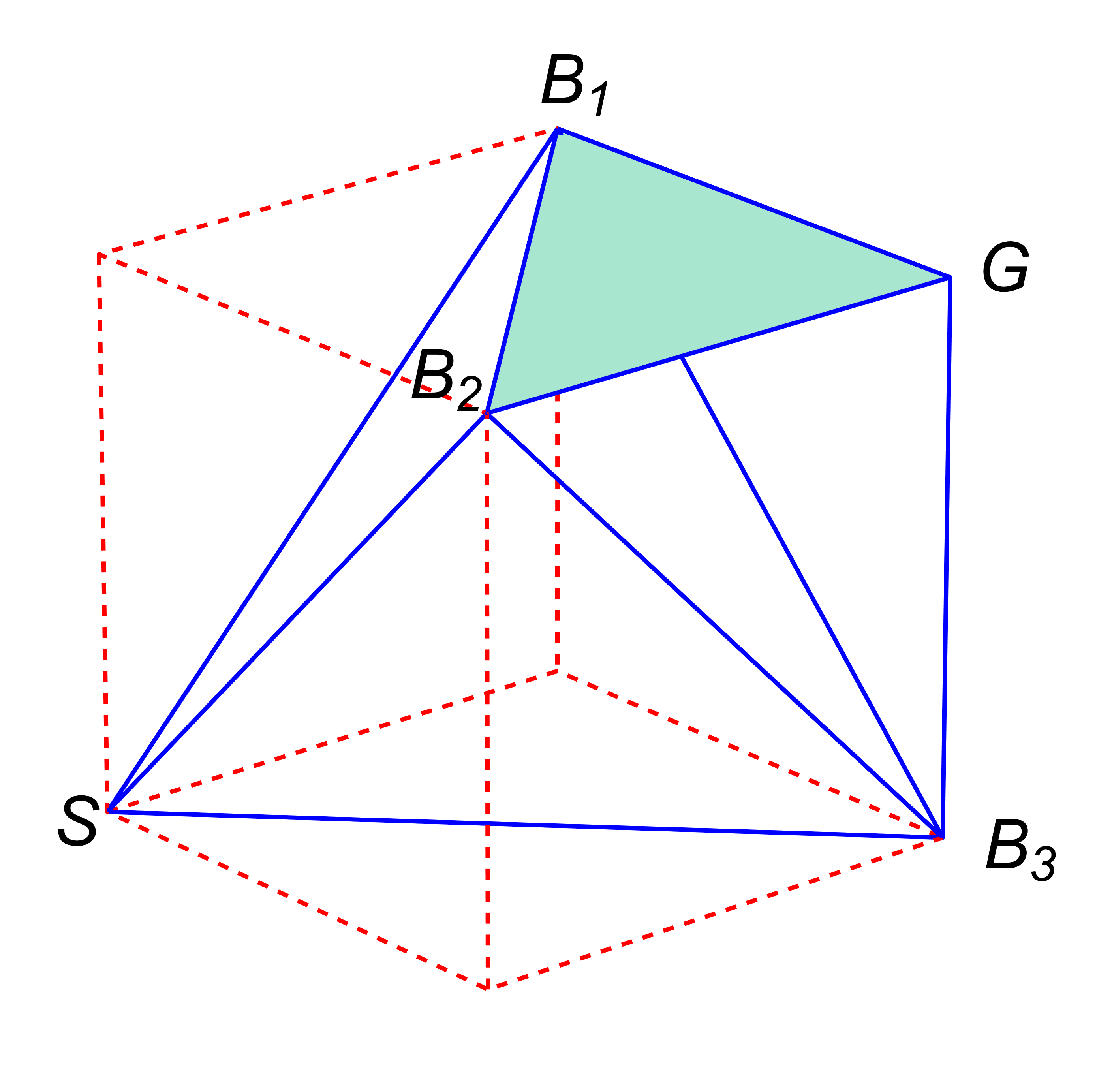
(c) Type 4c-3

Figure 5: The type 4c-$i$ states, $i=1,2,3$, are associated with the faces of the upper tetrahedron of the polytope $\mathcal{P}$.

The type 4d includes vectors that are expressed in an alternative canonical form [35],

$$|\psi_{4d}\rangle=c_{0}|001\rangle+c_{1}|010\rangle+c_{2}|100\rangle+c_{3}|111\rangle,\quad c_{k}\geq 0,\quad\sum_{k=0}^{3}c_{k}^{2}=1.$$ (16)

This class of states is associated with points along the entire polytope $\mathcal{P}$. The relationship between types 4b, 4c and 4d, has been numerically studied in [25].

3 Quantitative characterization of entanglement

Consider two different points in the entanglement–polytope, $\vec{\lambda}_{\psi_{k}}\in\mathcal{P}$, $k=1,2$. We know that there is at least one state $|\psi_{k}\rangle$ in $\mathcal{H}$ that is associated with each $\vec{\lambda}_{\psi_{k}}$ through the mapping $\Lambda$.

Assuming that $|\psi_{1}\rangle$ and $|\psi_{2}\rangle$ have a certain degree of entanglement, what it does mean to say that one of them is more entangled than the other?

The notion of entanglement measure gives diverse quantitative answers to such a question [2, 3, 4, 5, 9, 10, 44]. Most of them are based on the distance measures of quantum states, which quantify how close two states are (static case), or how well information has been preserved during a dynamic process (dynamic case) [1]. In any case, it is required a measure standard, a state (or set of states) for which the measure is equal to 1, and a state (or set of states) that provides a result equal to 0. For three-qubit entanglement, it is usual to associate $|GHZ\rangle$ with measure 1, and the fully separable states with measure 0. Within this standard, any entanglement measure of the states included in Table 1 should range between 0 and 1.

How do the entanglement properties of $|\psi_{k}\rangle$ affect point $\vec{\lambda}_{\psi_{k}}$?

Suppose $|\psi_{1}\rangle$ is the GHZ–state and that $|\psi_{2}\rangle$ is to be determined. Since $|GHZ\rangle$ corresponds to the vertex $\vec{G}=\vec{\lambda}_{\psi_{1}}$, if we wanted $|\psi_{2}\rangle$ to be as entangled as possible, we would look for the point $\vec{\lambda}_{\psi_{2}}$ to be in the vicinity of $\vec{G}$. The closer $\vec{\lambda}_{\psi_{2}}$ is to $\vec{G}$, the state $|\psi_{2}\rangle$ will be more ‘similar’ to $|GHZ\rangle$.

The problem is to define the notion of proximity between two points in $\mathcal{P}$ that corresponds to some entanglement measure in $\mathcal{H}$.

Next, we provide two different options, one addressed to quantify global entanglement and the other characterizing genuine entanglement.

Let us project the vector $\vec{\lambda}_{\psi}\in\mathcal{P}$ on the line segments $\overline{SB_{i}}\subset\mathcal{P}$. In each case one has

$$\vec{\lambda}_{\psi}=\vec{p}_{i}+\vec{q}_{i},\quad\vec{p}_{i}=\left(\vec{\lambda}_{\psi}\cdot\mathbf{e}_{B_{i}}\right)\mathbf{e}_{B_{i}},\quad\mathbf{e}_{B_{i}}=\sqrt{2}\vec{B}_{i},\quad i=1,2,3.$$ (17)

The above decomposition is illustrated in Figure 6. Vectors $\vec{p}_{i}$ and $\vec{q}_{i}$ are the projection of $\vec{\lambda}_{\psi}$ on $\vec{B}_{i}$ and rejection of $\vec{\lambda}_{\psi}$ from $\vec{B}_{i}$, respectively. Their norms, written in terms of the components of $\vec{\lambda}_{\psi}$, read as follows

$$p_{i}=\tfrac{1}{\sqrt{2}}\left(\lambda_{j}+\lambda_{k}\right),\quad q_{i}=\sqrt{\lambda_{i}^{2}+\tfrac{1}{2}\left(\lambda_{j}-\lambda_{k}\right)^{2}},\quad i,j,k=1,2,3.$$ (18)

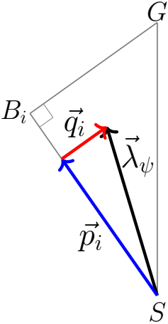
Figure 6: Partial section of the entanglement–polytope $\mathcal{P}$ along the plane $\Pi_{i}$ defined by the vertices $\vec{S}$, $\vec{B}_{i}$ and $\vec{G}$. The orthogonal projection of $\vec{\lambda}_{\psi}\in\mathcal{P}$ on the line-segment $\overline{SB_{i}}\subset\mathcal{P}$ (written $\vec{p}_{i}$), as well as the rejection of $\vec{\lambda}_{\psi}$ from $\overline{SB_{i}}$ (denoted $\vec{q}_{i}$) are useful for introducing diverse entanglement measures (see discussion in the main text). If $\vec{\lambda}_{\psi}$ is located in $\Pi_{i}$ (as shown in the figure), then $\vec{q}_{i}$ is also located in $\Pi_{i}$. In general, both $\vec{q}_{i}$ and $\vec{\lambda}_{\psi}$ localize the same (arbitrary) point of $\mathcal{P}$, the former from $\vec{p}_{i}$ on the line-segment $\overline{SB_{i}}$, the latter from the vertex $\vec{S}$.

Clearly $\vec{\lambda}_{\psi}=\vec{S}$ produces $p_{i}=q_{i}=0$, since $\lambda_{i}=0$ for all $i=1,2,3$. Avoiding this simple case, the identity $\vec{\lambda}_{\psi}=\vec{B}_{i}$ for some $i=1,2,3$, provides null rejection $q_{i}=0$, and vice versa. We have seen already that these points, distributed along the line segment $\overline{SB_{i}}$, yield the bi-separable states $|\psi_{\operatorname{bi}}\rangle=\ket{\phi_{i}}\ket{\phi_{jk}}$.

On the other hand, if $\lambda_{i}=\lambda$ for all $i=1,2,3$, then $p_{i}=\sqrt{2}\lambda$ and $q_{i}=\lambda$. Vectors $\vec{\lambda}_{\psi}$ satisfying this condition localize points along the line-segment $\overline{SG}$. In this case, the largest rejection $q_{i}=\nicefrac{{1}}{{2}}$ and largest projection $p_{i}=\nicefrac{{1}}{{\sqrt{2}}}$ are attributed to the vertex $\vec{\lambda}_{\psi}=\vec{G}$, see Figure 6.

It is notable that the norm of the projection $\vec{p}_{i}$ is proportional to the average (arithmetic mean) of $\lambda_{j}$ and $\lambda_{k}$, we write $p_{i}=\sqrt{2}\operatorname{Av}(\lambda_{j},\lambda_{k})$. Although the eigenvalue $\lambda_{i}$ seems to be missing here, it plays a significant role to define the decomposition (17). Indeed, $\lambda_{i}$ determines the length of $q_{i}$ (and the length of $p_{i}$ as well).

If we make $\lambda_{i}=0$, the inequalities (3) imply $\lambda_{j}=\lambda_{k}\equiv\lambda$ (by necessity), so that $q_{i}=0$. That is, as noted above, $\lambda_{i}=0$ produces the bi-separability of the three-qubit state by isolating the $i$th qubit. Moreover, if $\lambda_{i}=0$ then $p_{i}=\sqrt{2}\lambda$. Therefore $p_{i}\in[0,\nicefrac{{1}}{{\sqrt{2}}}]$, as expected for the bi-separable states $|\psi_{\operatorname{bi}}\rangle=\ket{\phi_{i}}\ket{\phi_{jk}}$.

In addition, since $\lambda_{i}=\nicefrac{{1}}{{2}}$ means that $\rho_{i}$ is maximally mixed, the corresponding three-qubit state (in the bipartition $i-jk$) is maximally entangled. This configuration imposes the number $\nicefrac{{1}}{{(2\sqrt{2})}}$ as a lower bound on the values of $p_{i}$, for which we find maximally entangled states. As a consequence, the projection domain is restricted to the second half of the previous case, $p_{i}\in[\nicefrac{{1}}{{(2\sqrt{2})}},\nicefrac{{1}}{{\sqrt{2}}}]$.

The previous analysis shows that the norm of $\vec{p}_{i}$ encodes sensitive information about the entanglement of the three-qubit system.

Looking for a global treatment, where all the components of $\vec{\lambda}_{\psi}$ intervene at the same time, we propose the following arithmetic mean

$$\xi(\psi)=\tfrac{\sqrt{2}}{3}\left(p_{1}+p_{2}+p_{3}\right)=\tfrac{2}{3}\left(\lambda_{1}+\lambda_{2}+\lambda_{3}\right),$$ (19)

which vanishes for fully separable states ($\lambda_{1,2,3}=0$), and is normalized to 1 for the GHZ–state ($\lambda_{1,2,3}=\nicefrac{{1}}{{2}}$).

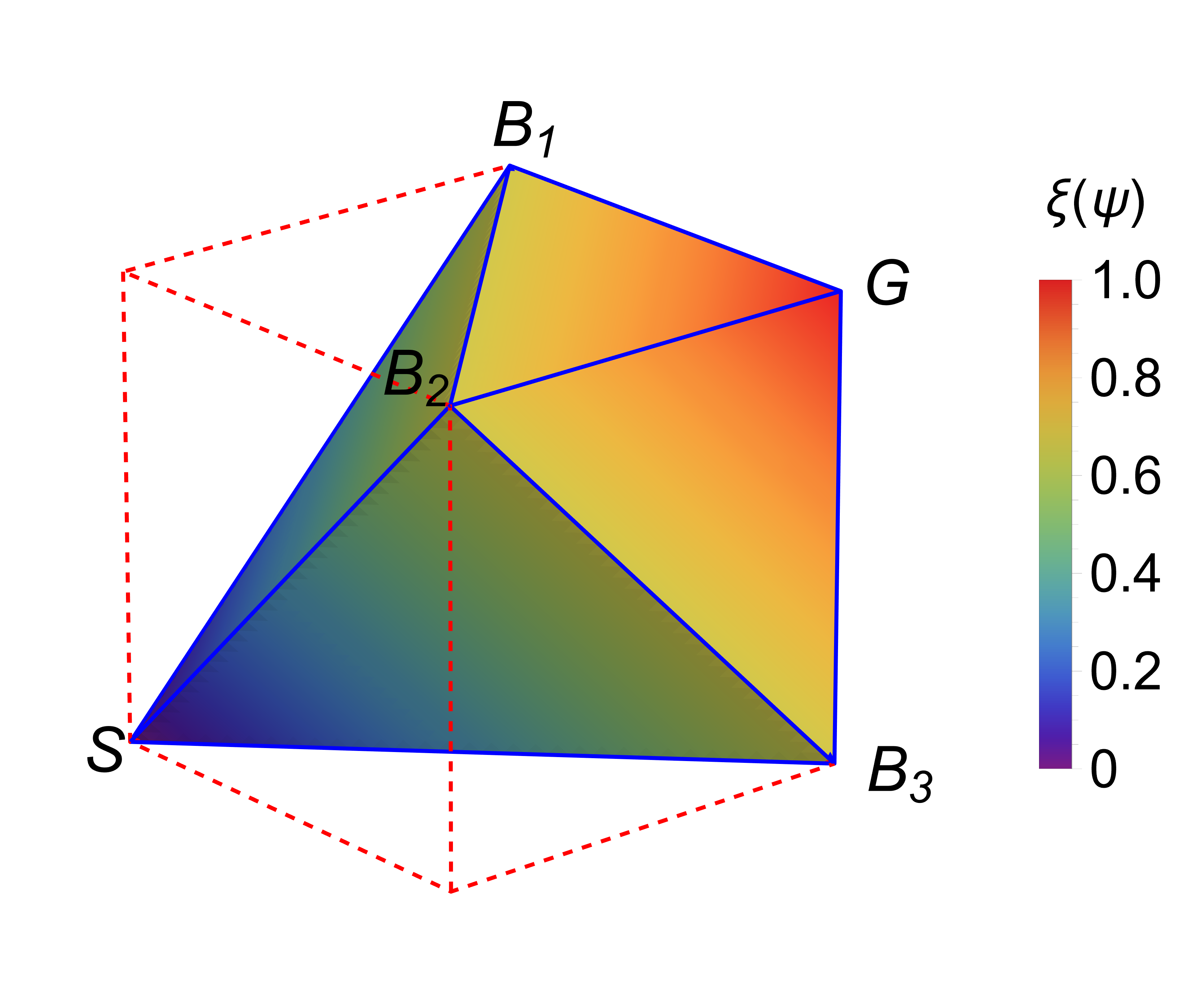
(a)

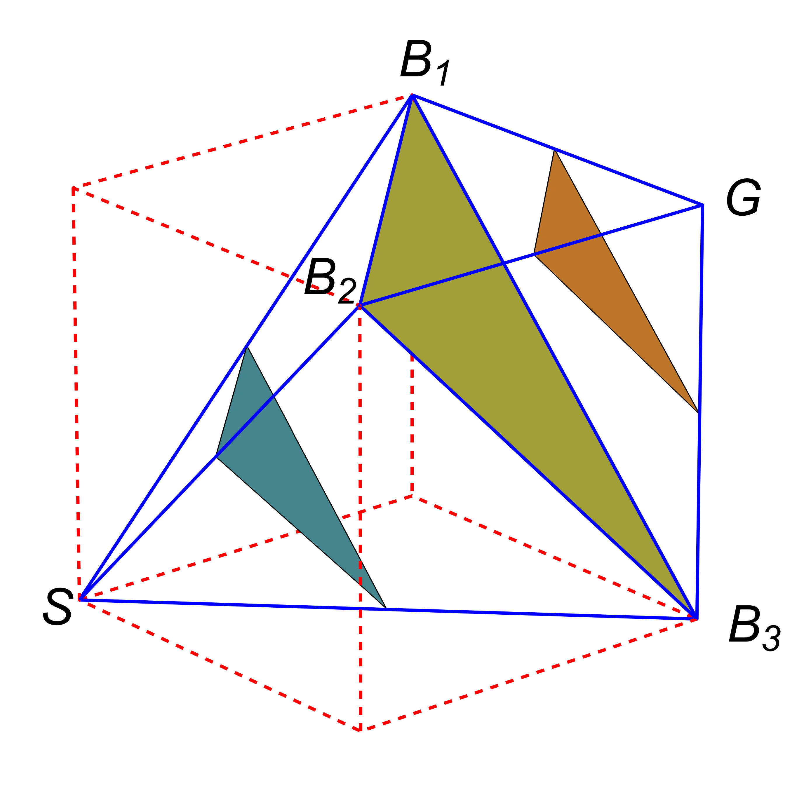
(b)

Figure 7: The arithmetic mean $\xi(\psi)$ introduced in Eq. (19) vanishes for fully separable states and is normalized to 1 for the GHZ–state. (a) The points $\vec{\lambda}_{\psi}\in\mathcal{P}$ average better values $\xi$ as they get closer to the vertex $\vec{G}\in\mathcal{P}$. (b) Condition $\xi(\psi)=\xi_{0}$, with $\xi_{0}=\operatorname{constant}$, defines planes transverse to the line segment $\overline{SG}$ whose points represent states $|\psi\rangle\in\mathcal{H}$ with the same degree of entanglement. The $\xi_{0}$–planes shown in the figure correspond to $\xi_{0}=\nicefrac{{1}}{{3}},\nicefrac{{2}}{{3}}$, and $\nicefrac{{5}}{{6}}$.

Figure 7(a) shows the distribution of points $\vec{\lambda}_{\psi}$ according to $\xi(\psi)$. Clearly, these points average better values $\xi$ as they get closer to the vertex $\vec{G}$.

Of particular interest, if $\lambda_{i}=\lambda$ for all $i=1,2,3$, then $p_{i}=\sqrt{2}\lambda$, $q_{i}=\lambda$, and $\xi(\psi)=2\lambda$. In this case $\vec{\lambda}_{\psi}$ localizes points along the line-segment $\overline{SG}$. Then the projection $p_{i}$ ($=\nicefrac{{1}}{{\sqrt{2}}}$), the rejection $q_{i}$ ($=\nicefrac{{1}}{{2}}$) and the measure $\xi$ ($=1$) reach their maximum when $\vec{\lambda}_{\psi}=\vec{G}$.

A very versatile property of the average (19) arises by imposing the condition $\xi(\psi)=\operatorname{constant}$, since this defines a plane transverse to the line segment $\overline{SG}$ whose points represent states $|\psi\rangle\in\mathcal{H}$ with the same degree of entanglement. Indeed, assume that such a plane cuts the line segment $\overline{SG}$ at the point localized by $\vec{\lambda}_{0}$. We write $\vec{\lambda}_{0}=\xi_{0}\vec{G}$, with $\xi_{0}\in[0,1]$. If $\vec{\lambda}$ localizes another point on the plane, then $\vec{\lambda}-\vec{\lambda}_{0}$ must be orthogonal to the unitary vector $\mathbf{n}=||\vec{G}||^{-1}\vec{G}$, so we arrive at the equation

$$\hat{n}\cdot(\vec{\lambda}-\vec{\lambda}_{0})=0.$$ (20)

The solution of (20) is easily found, it is given by $\xi_{0}=\xi(\psi)$.

Figure 7(b) shows some $\xi_{0}$–planes. Among them, the triangle $\triangle_{B_{1}B_{2}B_{3}}$ coincides with the plane $\xi_{0}=\nicefrac{{2}}{{3}}$ and contains the W–state at its geometric center, as indicated above. That is, $|W\rangle$ is $\xi=\nicefrac{{1}}{{3}}$ distant from $|GHZ\rangle$.

The decomposition (17) offers another possibility to quantify entanglement. As we have seen, the rejection $\vec{q}_{i}$ is very sensitive to the eigenvalue $\lambda_{i}$ (its norm $q_{i}$ cancels if $\lambda_{i}=0$), and vice versa. Then, we may use $q_{i}$ to quantify the ‘transverse distance’ between $\vec{\lambda}_{\psi}$ and $\overline{SB_{i}}$ since vector $\vec{\lambda}_{\psi}$ is as ‘close’ to $\overline{SB_{i}}$ as the rejection $q_{i}$ (equivalently, $\lambda_{i}$) approaches zero. In this context, we introduce the function

$$\mu(\psi)=2\min(q_{1},q_{2},q_{3}),$$ (21)

which quantifies the transverse–distance from $\vec{\lambda}_{\psi}$ to the nearest line segment $\overline{SB_{i}}$.

Figure 8 shows the distribution of points $\vec{\lambda}_{\psi}$ according to the function $\mu$.

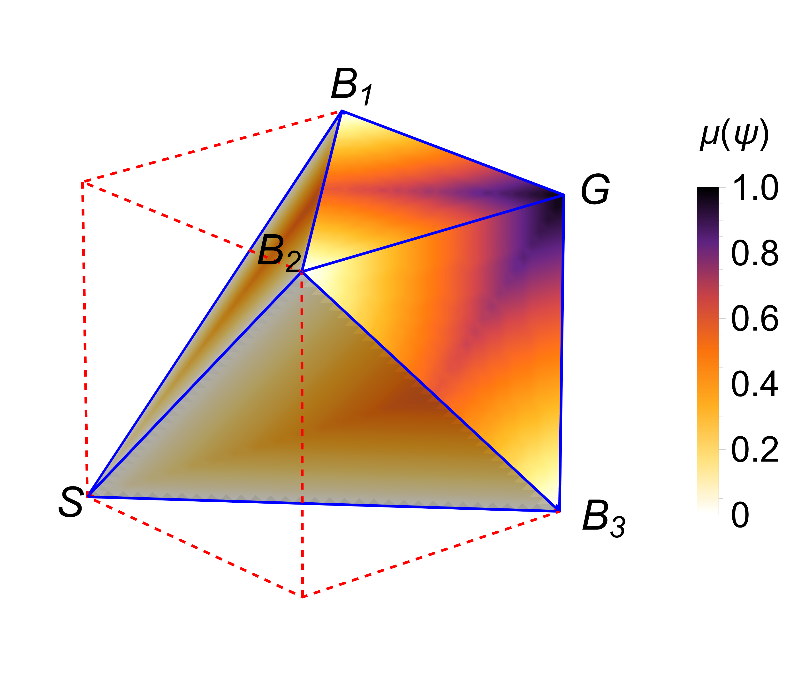
Figure 8: The transverse–distance measure $\mu(\psi)$ introduced in (21) gives 0 for separable states and 1 for the GHZ–state. In addition, this also gives 0 for bi-separable states, so it discriminates bi-separability from genuine entanglement. Notably, $\mu$ gives the same value as $\xi$ for the W–state, which confirms that $|W\rangle$ is $\xi=\mu=1/3$ distant from $|GHZ\rangle$.

The standard of $\mu(\psi)$ is as follows: it vanishes for separable states, attains its maximum value ($=1$) for the GHZ–state, and carries out the value $\mu=\nicefrac{{2}}{{3}}$ for the W–state. Incidentally, $\mu(\psi)$ gives the same value as $\xi(\psi)$ for the W–state, reinforcing our previous statement that $|W\rangle$ is $\xi=\mu=\nicefrac{{1}}{{3}}$ distant from $|GHZ\rangle$, see Figure 9.

As $q_{i}=0$ is a condition for bi-separability, in contrast with $\xi$, the measure $\mu$ also gives the value 0 for bi-separable states, see Figure 9. Indeed, $\mu$ is a measure of genuine multipartite entanglement since it satisfies the requirements reported in, for example, [18].

Figure 9 shows the values provided by the measures $\xi$ and $\mu$ for states $|\psi_{\operatorname{sep}}\rangle$, $|\psi_{\operatorname{bi}}\rangle=|0\rangle_{i}|\psi^{+}\rangle_{jk}$, $|W\rangle$ and $|GHZ\rangle$. These results are compared with the values that can be obtained in terms of the concurrence–fill $F_{123}$ [18] and the genuine multipartite concurrence $\mathcal{C}_{\operatorname{GME}}$ [19]. With exception of $\xi$, these measures give 0 for bi-separable states. That is, $\xi$ does not discriminate bi-separability from genuine entanglement, so it is a measure of global entanglement. On the other hand, among these measures, $\mu$ averages the lowest results for the four states. In other words, $\mu$ defines a lower bound for measuring genuine entanglement.

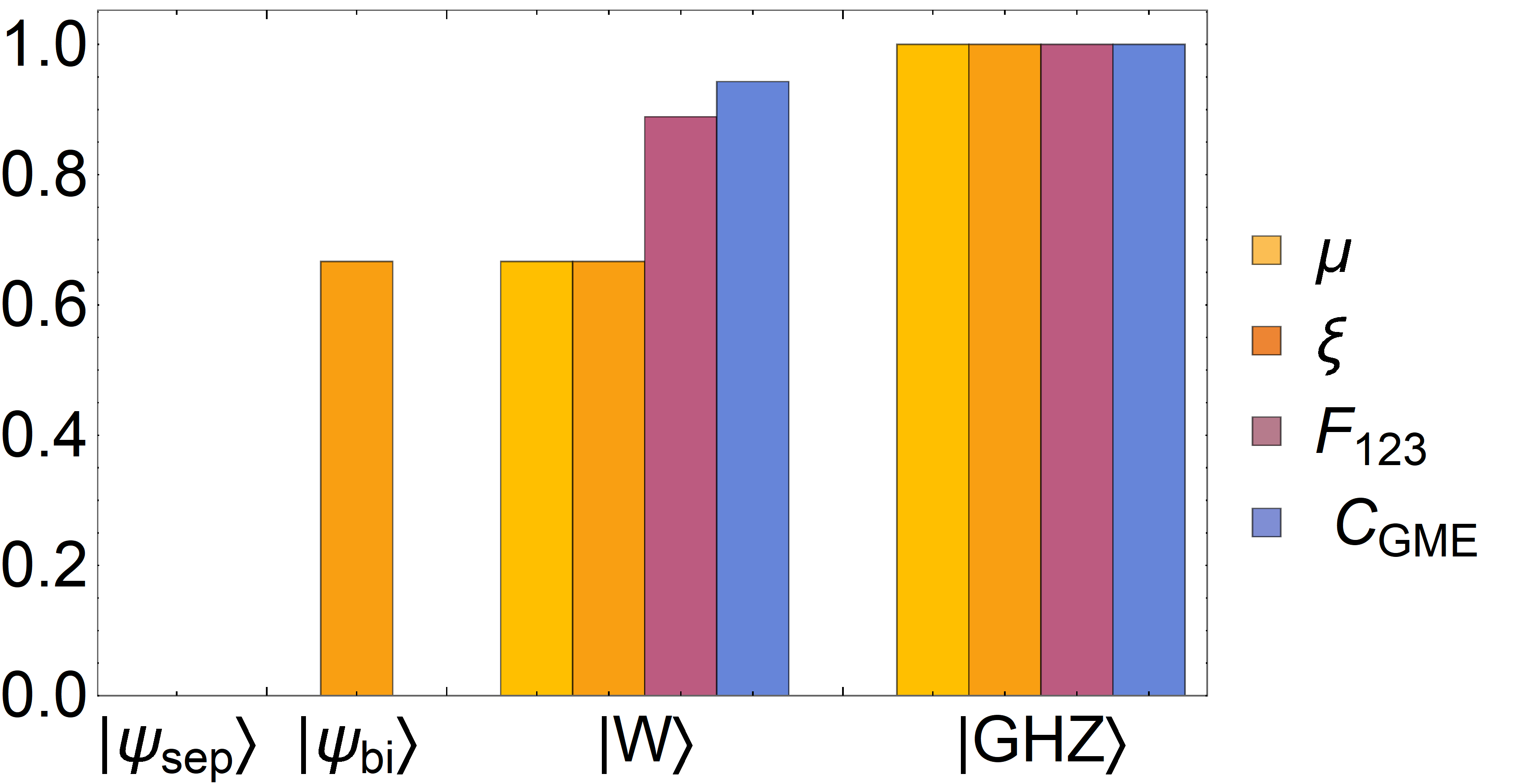
Figure 9: Entanglement measures $\xi(\psi)$, $\mu(\psi)$, $F_{123}(\psi)$ and $\mathcal{C}_{GME}(\psi)$ for states $|\psi_{\operatorname{sep}}\rangle$, $|\psi_{\operatorname{bi}}\rangle=|0\rangle_{i}|\Psi^{+}\rangle_{jk}$, $|W\rangle$ and $|GHZ\rangle$. All the measures give 0 for fully separable states. Measure $\xi$ does not discriminate bi-separability from genuine entanglement since it averages a value different from 0 for bi-separable states. Among these measures, $\mu$ gives the lowest results for the four states.

To compare in more detail both the properties and the behavior of the measures $\xi$ and $\mu$, let us consider the type 3a state

$$|\psi_{\alpha}\rangle=\cos\alpha|100\rangle+\sin\alpha|0\rangle_{1}|\Psi^{+}\rangle_{23},\quad 0\leq\alpha\leq\tfrac{\pi}{2}.$$ (22)

It is a matter of substitution to verify that $|\psi_{\alpha=0}\rangle=|100\rangle$ and $|\psi_{\alpha=\pi/2}\rangle=|0\rangle_{1}|\Psi^{+}\rangle_{23}$. That is, at the ends of the $\alpha$-domain, the state $|\psi_{\alpha}\rangle$ becomes fully separable and bi-separable, respectively. Additionally, making $\alpha=\alpha_{0}=\arccos(\nicefrac{{1}}{{\sqrt{3}}})$, one gets $|\psi_{\alpha_{0}}\rangle=|W\rangle$.

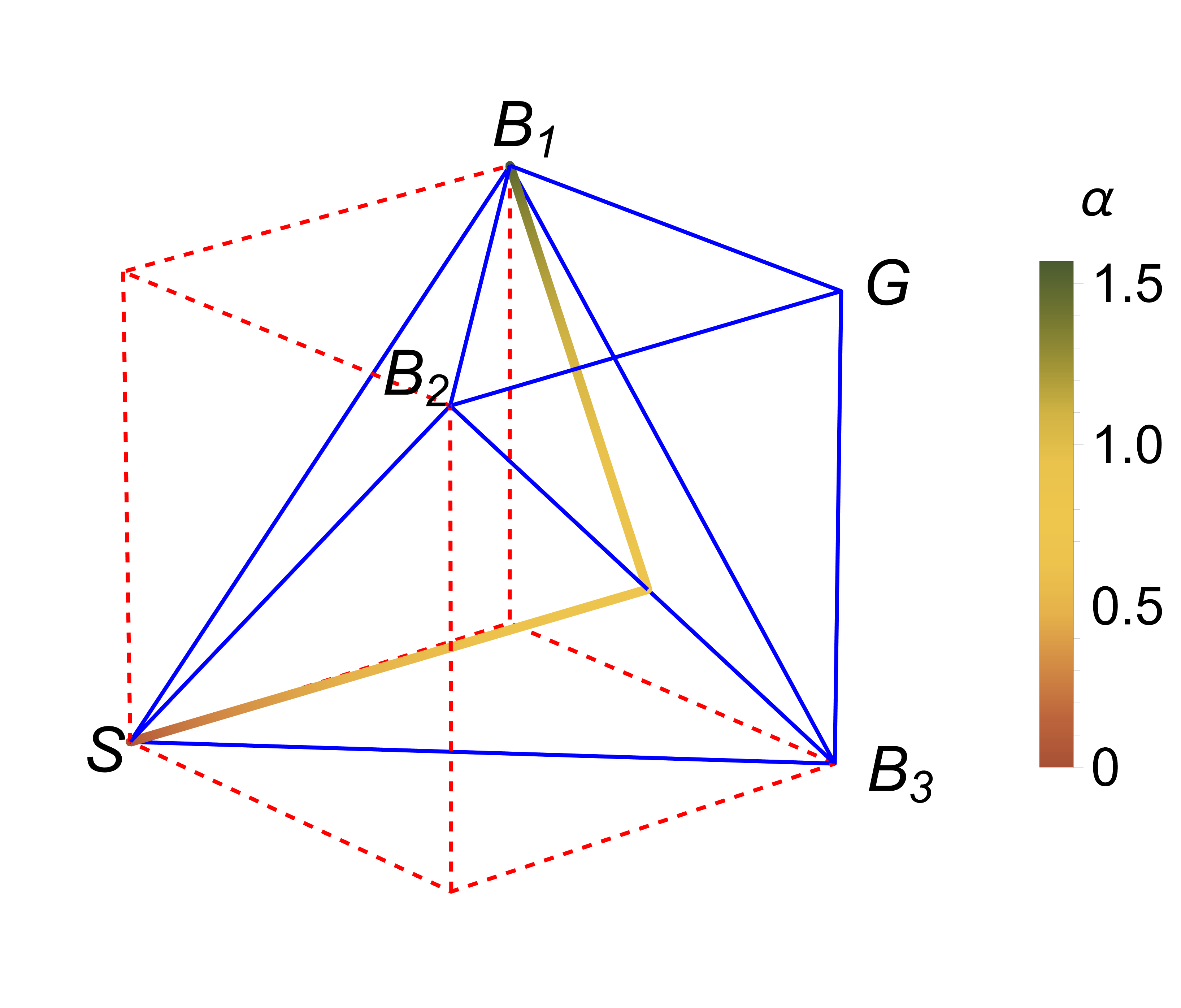
(a)

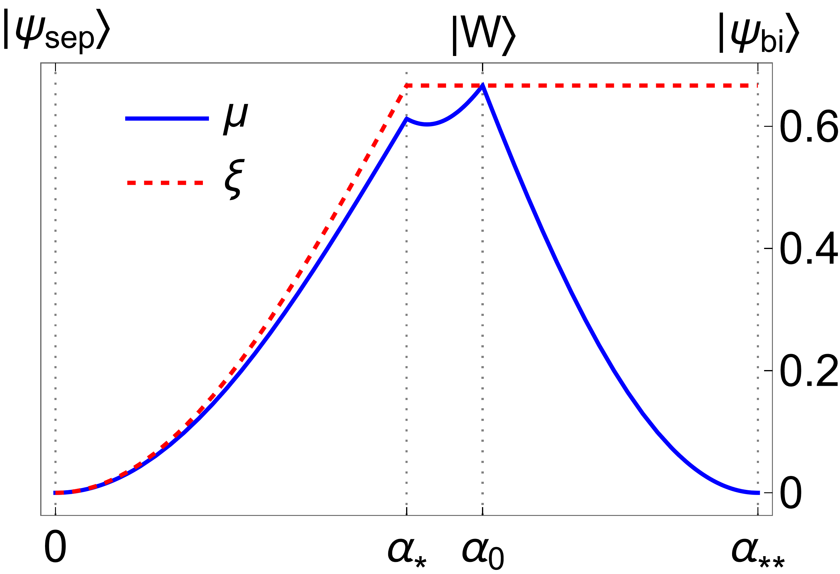
(b)

Figure 10: (a) When the parameter $\alpha$ sweeps the domain $[0,\alpha_{**}]\equiv[0,\pi/2]$, the state $|\psi_{\alpha}\rangle$ introduced in (22) describes a path $\vec{\lambda}_{\psi_{\alpha}}$ on the lower tetrahedron of $\mathcal{P}$. The trajectory goes first from the vertex $\vec{S}$ to the midpoint of $\overline{B_{2}B_{3}}$ (at $\alpha=\alpha_{*}=\pi/4$), and then to the vertex $\vec{B}_{1}$ (at $\alpha=\alpha_{**}$) on the triangle $\triangle_{B_{1}B_{2}B_{3}}$. In this last journey, $\vec{\lambda}_{\psi_{\alpha}}$ passes through the geometric center of $\triangle_{B_{1}B_{2}B_{3}}$, at $\alpha=\alpha_{0}=\arccos(\nicefrac{{1}}{{\sqrt{3}}})$, which houses state $|W\rangle$. (b) Measures $\xi$ and $\mu$ for state $|\psi_{\alpha}\rangle$, the former gives $\xi_{0}=2/3$ for $\alpha\in[\alpha_{*},\alpha_{**}]$ whereas the latter cancels at the ends of the $\alpha$-domain. In contrast with $\xi$, the measure $\mu$ also distinguishes among the points living on $\triangle_{B_{1}B_{2}B_{3}}$. That is, points $\vec{\lambda}_{\psi_{\alpha}}$ closer to the center of $\triangle_{B_{1}B_{2}B_{3}}$ will correspond to more $\mu$-entangled states $|\psi_{\alpha}\rangle$.

Parameterized by $\alpha$, the vector $\vec{\lambda}_{\psi_{\alpha}}$ describes a path in the entanglement–polytope $\mathcal{P}$ that follows a trajectory from $\vec{S}$ (at $\alpha=0$) to $\vec{B}_{1}$ (at $\alpha=\pi/2$), see Figure 10(a). Looping through values in the first half of the $\alpha$-domain, $\vec{\lambda}_{\psi_{\alpha}}$ draws a straight line on the triangle $\triangle_{SB_{2}B_{3}}$, from $\vec{S}$ to the midpoint of segment $\overline{B_{2}B_{3}}$ (at $\alpha=\pi/4$). From there, the vector continues in a straight line on triangle $\triangle_{B_{1}B_{2}B_{3}}$ to vertex $\vec{B}_{1}$. In this last journey, $\vec{\lambda}_{\psi_{\alpha}}$ passes through the geometric center of $\triangle_{B_{1}B_{2}B_{3}}$ (at $\alpha=\alpha_{0}$), which houses state $|W\rangle$.

Remember that mesure $\xi$ averages the constant value $\xi_{0}=2/3$ for any point on the triangle $\triangle_{B_{1}B_{2}B_{3}}$, see Figure 7(b). Then, the values averaged by $\xi$ would indicate that the degree of entanglement of $|\psi_{\alpha}\rangle$ is conserved during the second part of the path described above, just as it is shown in Figure 10(b). In turn, $\mu$ gives 0 for both separable and bi-separable states, so it cancels at the ends of the $\alpha$-domain. That is, with the values given by $\mu$ we find that $|\psi_{\alpha}\rangle$ increases its degree of entanglement during the first half of the journey, and decreases it during the second half to remain as at the beginning. According to $\mu$, the maximum degree of entanglement is reached at $\alpha=\alpha_{0}$, where $|\psi_{\alpha}\rangle$ coincides with $|W\rangle$. Indeed, $\mu$ averages two local maxima, the one at $\alpha=\alpha_{0}$, and another at $\alpha=\alpha_{*}=\pi/4$, see Figure 10(b). Between $\alpha_{*}$ and $\alpha_{0}$ (the transit from $\overline{B_{2}B_{3}}$ to the geometric center of $\triangle_{B_{1}B_{2}B_{3}}$) there is still an increase of $\mu$ that connects these maxima. This last result shows that, in contrast with $\xi$, the measure $\mu$ also distinguishes among the points living on $\triangle_{B_{1}B_{2}B_{3}}$. The points $\vec{\lambda}_{\psi_{\alpha}}$ closer to the center of $\triangle_{B_{1}B_{2}B_{3}}$ will correspond to more $\mu$-entangled states $|\psi_{\alpha}\rangle$.

Let us verify the universality of measure $\mu$ to quantify genuine multipartite entanglement. Consider the state

$$|\psi_{\theta}\rangle=N(\theta)\left[\cos^{2}\left(\tfrac{\theta}{2}\right)|111\rangle+\tfrac{1}{\sqrt{3}}\sin^{2}\left(\tfrac{\theta}{2}\right)|W\rangle\right],\quad\theta\in[0,\pi],$$ (23)

where

$$N(\theta)=\left[\cos^{4}\left(\tfrac{\theta}{2}\right)+\tfrac{1}{3}\sin^{4}\left(\tfrac{\theta}{2}\right)\right]^{-1/2}$$

stands for the normalization constant. It is immediate to verify the identities $|\psi_{\theta=0}\rangle=|111\rangle$, $|\psi_{\theta=\pi}\rangle=|W\rangle$ and $|\psi_{\theta=\theta_{0}}\rangle=|\varphi\rangle$, with $\theta_{0}=2\pi/3$. The latter state is given in Eq. (31), which has been shown to be local unitary equivalent to the GHZ–state. The measures $\mu$ and $F_{123}$ are respectively given by

$$\mu(\psi_{\theta})=1-\frac{2}{3}\bigg{|}\frac{3+5\cos\theta+\cos 2\theta}{3+2\cos\theta+\cos 2\theta}\bigg{|},$$ (24)

and

$$F_{123}(\psi_{\theta})=\frac{8(16\cos\theta+5\cos 2\theta+15)}{9(2\cos\theta+\cos 2\theta+3)}\sin^{4}\left(\frac{\theta}{2}\right).$$ (25)

In turn, the GME–concurrence reads $\mathcal{C}_{\operatorname{GME}}(\psi_{\theta})=\sqrt{F_{123}(\psi_{\theta})}$.

The above functions are plotted in Figure 11. They range between 0 and 1, with $\mu$ defining the lower bound for any $\theta\neq\theta_{0}$. At $\theta_{0}$, the three measures give the result 1.

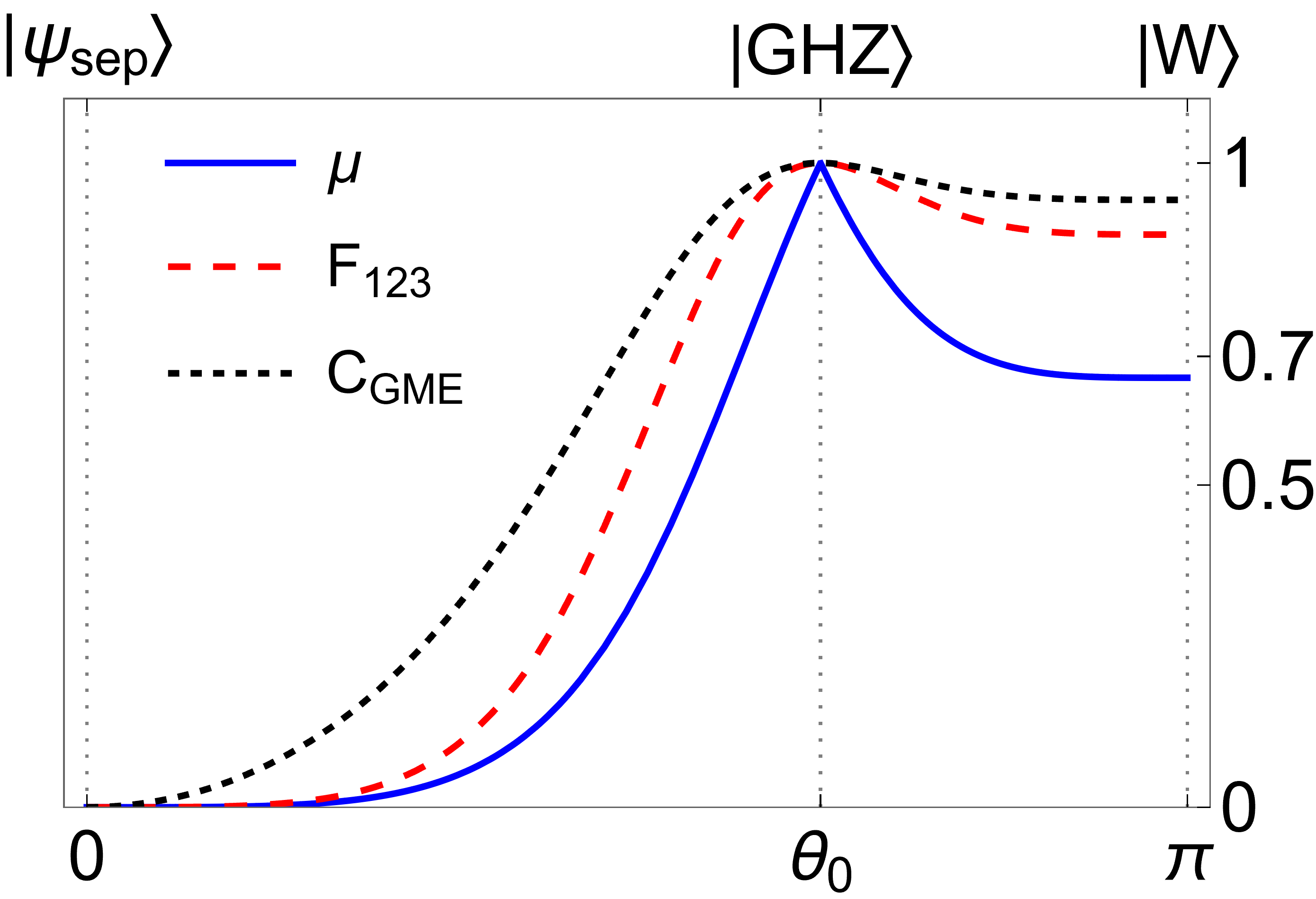
Figure 11: Entanglement measures $\mu(\psi)$, $F_{123}(\psi)$ and $\mathcal{C}_{\operatorname{GME}}(\psi)$ for the state $|\psi_{\theta}\rangle$ given in Eq. (23). At $\theta=0$ the state becomes $|111\rangle$, so it is fully separable. However, it is maximally entangled at $\theta=\theta_{0}=2\pi/3$, since it is local unitary equivalent to the GHZ–state. At $\theta=\pi$ the state is equal to $|W\rangle$. Consistently, the measures range between 0 and 1, reaching their maximum ($=1$) at $\theta_{0}$. Measure $\mu$ defines a lower bound, as it produces lower values than the results of the other two measures, except at $\theta=\theta_{0}$.

Note that $\mu$ defines a lower bound on the degree of entanglement that could be measured in the state $|\psi_{\theta}\rangle$, as it produces lower values than the results of the other two measures.

4 The inverse problem

One of the advantages of working with the geometric representation of quantum states is that the classification of entanglement becomes visual and simple. If a given three-qubit state $|\psi\rangle\in\mathcal{H}$ exhibits a certain amount of entanglement, this is linked to a very concrete point of the entanglement–polytope $\mathcal{P}$ throughout the vector $\vec{\lambda}_{\psi}$.

The question in the opposite direction offers even more interesting challenges and a much broader perspective on entanglement.

Given a point $\vec{\lambda}\in\mathcal{P}$, what three-qubit state (or class of states) can be mapped from $\mathcal{H}$ to precisely $\vec{\lambda}$?

This dilemma is an example of the inverse problem of quantum mechanics [36], where one seeks to manipulate systems in order to force them to behave in a particular way (some applications can be found in [37, 38, 39, 40, 41, 42]). In the present case, it is about choosing a point of the polytope in a region that characterizes very specific entanglement properties, and searching for the quantum state that satisfies such a profile.

Some of the possibilities of the inverse problem for states of types 1 to 4a have been explored in [24] (although the authors of such work do not use the terminology of the inverse problem nor exploit all the potential of the method). However, as a matter of fact, the solutions to the inverse problem for three-qubit systems are far from being exhausted. For example, to the best of our knowledge, the inverse problem for the facets $B_{1}B_{2}G$, $B_{1}B_{3}G$ and $B_{2}B_{3}G$, remains unsolved.

To contribute to this topic, let us solve the problem of determining the states that can be associated with a given point $\vec{\lambda}$ on the triangle $\triangle_{B_{2}B_{3}G}\in\mathcal{P}$.

The states that we are looking for belong to type 4c-1, so they are written in the form of Eq. (12). Since $\vec{\lambda}_{\psi_{4c-1}}$ must be provided in advance, we assume that we know every one of the coefficients of the convex combination (13). Then, we solve the parameter system (14) to fix the coefficients of $|\psi_{4c-1}\rangle$ in (12). The acceptable solutions are as follows

$$\begin{array}[]{l}b_{2}^{2}=\frac{1}{4}\left(1+\kappa_{1}^{2}-\kappa_{2}^{2}-\sqrt{\left(1-\kappa_{1}^{2}+\kappa_{2}^{2}\right)^{2}-4\kappa_{2}^{2}}\right),\\[10.33333pt] b_{3}^{2}=\frac{1}{4}\left(1-\kappa_{1}^{2}+\kappa_{2}^{2}-\sqrt{\left(1-\kappa_{1}^{2}+\kappa_{2}^{2}\right)^{2}-4\kappa_{2}^{2}}\right),\\[10.33333pt] b_{4}^{2}=\frac{1}{2}\left(1-\sqrt{\left(1-\kappa_{1}^{2}+\kappa_{2}^{2}\right)^{2}-4\kappa_{2}^{2}}\right).\end{array}$$ (26)

Thus, coefficients (26) are determined by the parametrization $\kappa_{1}$, $\kappa_{2}$ and $1-\kappa_{1}-\kappa_{2}$, which also defines the facet $B_{2}B_{3}G$.

The inverse problem for facets $B_{1}B_{3}G$ and $B_{1}B_{2}G$ finds a similar solution, this time using the states (15).

In a more general picture, any point $\vec{\lambda}\in\mathcal{P}$ can be written as a convex combination of the extremal points,

$$\vec{\lambda}=\kappa_{0}\vec{S}+\kappa_{1}\vec{B}_{1}+\kappa_{2}\vec{B}_{2}+\kappa_{3}\vec{B}_{3}+\kappa_{4}\vec{G},\quad\kappa_{q}\geq 0,\quad\sum_{q=0}^{4}\kappa_{q}=1.$$ (27)

This expression is universal for three-qubit systems in the sense that any of the states reported in Table 1 can be associated with $\vec{\lambda}$.

For example, knowing that states of type 4d are mapped to points along the entire entanglement–polytope $\mathcal{P}$, let us consider $|\psi_{4d}\rangle$ as it is given in Eq. (16). Making $c_{r}^{2}=v_{r}$, the corresponding smallest eigenvalues are

$$\begin{array}[]{ll}\lambda_{1}=\frac{1}{2}\left[1-\sqrt{1-4(v_{2}+v_{3})\left(1-v_{2}-v_{3}\right)}\right],\\[8.00002pt] \lambda_{2}=\frac{1}{2}\left[1-\sqrt{1-4(v_{1}+v_{3})\left(1-v_{1}-v_{3}\right)}\right],\\[8.00002pt] \lambda_{3}=\frac{1}{2}\left[1-\sqrt{1-4(v_{0}+v_{3})\left(1-v_{0}-v_{3}\right)}\right].\end{array}$$ (28)

Since these eigenvalues define the vector $\vec{\lambda}$, from (27) and (28) we see that the coefficients of $|\psi_{4d}\rangle$ can be expressed in terms of $\kappa_{i}$, $i=0,1,2,3$, as follows

$$\begin{array}[]{cc}v_{0}=\frac{1}{2}\left[1-2v_{3}\pm(\kappa_{0}+\kappa_{3})\right],\quad v_{1}=\frac{1}{2}\left[1-2v_{3}\pm(\kappa_{0}+\kappa_{2})\right],\\[8.00002pt] v_{2}=\frac{1}{2}\left[1-2v_{3}\pm(\kappa_{0}+\kappa_{1})\right],\quad v_{3}+v_{2}+v_{1}+v_{0}=1.\end{array}$$ (29)

Only four of the set of solutions above are admissible for our purposes. In particular, the case ‘$+$’ yields

$$c_{0}^{2}=\tfrac{1}{2}\left(\kappa_{3}+\tfrac{\kappa_{4}}{2}\right),\quad c_{1}^{2}=\tfrac{1}{2}\left(\kappa_{2}+\tfrac{\kappa_{4}}{2}\right),\quad c_{2}^{2}=\tfrac{1}{2}\left(\kappa_{1}+\tfrac{\kappa_{4}}{2}\right),\quad c_{3}^{2}=\tfrac{1}{2}\left(1+\kappa_{0}-\tfrac{\kappa_{4}}{2}\right).$$ (30)

The set (30) constitutes the solution to the inverse problem of the entanglement–polytope $\mathcal{P}$ that we are dealing with. By providing purely geometric information, through the parameters $\kappa_{i}$, the state $|\psi_{4d}\rangle$ is completely determined, with very specific entanglement properties that can be defined on demand.

To verify the universality of the above solution, first consider the vertex $\vec{S}$. That is, $\kappa_{0}=1$. Then $c_{3}=1$ and $c_{0}=c_{1}=c_{2}=0$. In this case we arrive at the fully separable state $|111\rangle$. Another immediate example arises if $\kappa_{4}=1$ (the vertex $\vec{G}$), then $c_{0}=c_{1}=c_{2}=c_{3}=\nicefrac{{1}}{{2}}$, and

$$|\varphi\rangle=\frac{1}{2}\left(\sqrt{3}|W\rangle+|111\rangle\right).$$ (31)

This state is local unitary equivalent to the GHZ state. Indeed,

$$|\varphi\rangle=\left(\sigma_{x}H\otimes\sigma_{x}H\otimes\sigma_{x}H\right)|GHZ\rangle,$$

with $H$ the Hadamard operator.

More interesting configurations are obtained when two or more $\kappa$-parameters are different from zero. In the extreme case, where $\kappa_{i}\neq 0$ for all $i=0,1,2,3,4$, one can pay attention to the barycenter of the simplex $\triangle_{B_{1}B_{2}B_{3}}$ (where state $|W\rangle$ is located). The inverse problem solution leads to the state

$$|\chi\rangle=\tfrac{1}{\sqrt{2}}\left(|W\rangle+|111\rangle\right).$$ (32)

It is remarkable that $|\chi\rangle$ is not local unitary equivalent to $|W\rangle$, although these two states are mapped into the same point of the entanglement–polytope $\mathcal{P}$. The difference is notable considering that the three-tangle of $|W\rangle$ is equal to zero [43], while the three-tangle of $|\chi\rangle$ is equal to $4/(3\sqrt{3})$.

The above case shows the generality that the inverse problem introduces in the determination of quantum states. In the conventional (direct) problem, every state $|\psi\rangle\in\mathcal{H}$ is mapped to one and only one point of $\mathcal{P}$. However, the fact that two or more elements of $\mathcal{H}$ can be mapped to the same point of $\mathcal{P}$ usually goes unnoticed because, in the direct problem, attention is paid to a specific state. The inverse problem considers all possibilities in $\mathcal{H}$ that can be associated with $\vec{\lambda}\in\mathcal{P}$ in a single move. The latter means that the solution to the inverse problem usually associates a family of states, rather than a single state, with such a point.

As we have seen, the solution (30) provides universality to the state $|\psi_{4d}\rangle$ in Eq. (16). Once the coefficients $c_{k}$ of $|\psi_{4d}\rangle$ are parametrized with purely geometric information, obtained from the entanglement–polytope $\mathcal{P}$, the entanglement properties of such state become manipulable. Furthermore, the strength of set (30) lies in the fact that any other selection of solutions (29) is local unitary equivalent to (30). For example, taking the roots ‘$+,-,-$’, from (29) we have

$$c_{0}^{2}=\tfrac{1}{2}\left(1+\kappa_{0}-\tfrac{\kappa_{4}}{2}\right),\quad c_{1}^{2}=\tfrac{1}{2}\left(\kappa_{1}+\tfrac{\kappa_{4}}{2}\right),\quad c_{2}^{2}=\tfrac{1}{2}\left(\kappa_{2}+\tfrac{\kappa_{4}}{2}\right),\quad c_{3}^{2}=\tfrac{1}{2}\left(\kappa_{3}+\tfrac{\kappa_{4}}{2}\right).$$

The state $|\widetilde{\psi}_{4d}\rangle$ that results from these coefficients is local unitary equivalent to $|\psi_{4d}\rangle$ through the transformation $U_{1}=\sigma_{x}\otimes\sigma_{x}\otimes\mathds{1}$. Similarly, the roots ‘$-,+,-$’ and ‘$-,-,+$’ provide states of type 4d that can be transformed into the form $|\psi_{4d}\rangle$ by using the unitary operators $U_{2}=\sigma_{x}\otimes\mathds{1}\otimes\sigma_{x}$ and $U_{3}=\mathds{1}\otimes\sigma_{x}\otimes\sigma_{x}$, respectively.

We have chosen type 4d states to exemplify, in a more or less general way, the applicability and power of the inverse problem. Therefore, we must emphasize that this method is applicable to any point $\vec{\lambda}_{\psi}\in\mathcal{P}$, in connection with the states included in Table 1.

In general, the versatility of the solutions of the inverse method could extend to the practical aspects of entanglement. For example, the creation and measurement of three-qubit entanglement associated with states of type  4c-2 have been reported in [28]. Since these results are parametrized by data obtained from the optical bench in the laboratory, information like this could be translated to the entanglement–polytope $\mathcal{P}$ to give it measurable properties.

5 Conclusions

We have studied the degree of entanglement between the different parts of a tripartite qubit system from a purely geometric perspective. After constructing the convex polytope $\mathcal{P}\subset\mathbb{R}^{3}$ formed by the points $\vec{\lambda}=(\lambda_{1},\lambda_{2},\lambda_{3})$, where $\lambda_{k}$ is the smallest eigenvalue of the reduced matrix associated with the $k$th qubit [24, 23, 25, 26], we have considered the map $\Lambda:\mathcal{H}\rightarrow\mathcal{P}$ to identify some relationships between the tripartite quantum states $|\psi\rangle\in\mathcal{H}$ and the points of the projective space $\cal P$.

In agreement with the conditions reported in [24], we have shown that the classification of entangled states introduced in [7, 8] results in the identification of concrete subsets of $\mathcal{P}$ under the mapping $\Lambda$. The emphasis in the present study has been on the states mapped into the facets of the polytope $\mathcal{P}$.

Considering the geometric properties of the polytope $\mathcal{P}$, we have introduced two different entanglement measures, denoted $\xi$ and $\mu$. They are respectively associated with the projection and rejection of the point $\vec{\lambda}$ on the biseparable segments of $\mathcal{P}$; the former quantifies global entanglement while the latter measures genuine entanglement. When compared with some previously reported measures of entanglement, it is found that $\xi$ and $\mu$ establish a lower bound for the type of entanglement to which they refer (excluding the GHZ–state for which both measurements return the value 1, as would be expected).

The above results can be extended in several directions. For example, one may consider the projection of $\vec{\lambda}$ onto different subsets of $\mathcal{P}$ in such a way that different entanglement information is provided. In general, the definition of $\xi$ and $\mu$ can be directly extended to the multi-qubit case, since the points of the corresponding entanglement–polytope (the dimension of the space that contains it does not matter) can always be projected onto the appropriate subsets of biseparable points.

The advantages of working with the geometric representation of quantum states, as we have done here, become more evident when considering the possibility of controlling and manipulating entanglement.

As we have shown, by solving the inverse problem we can force the system to behave in a particular way. In particular, given a point of the polytope in a region that characterizes very specific entanglement properties, the quantum state that satisfies such a profile is sought. As a matter of fact, the solution to the inverse problem associates a family of states in $\mathcal{H}$, rather than a single state, with such a point. The latter provides information of the space of states $\mathcal{H}$ that cannot be obtained by solving the conventional (direct) problem, where a given state in $\mathcal{H}$ is mapped to one and only one point of $\mathcal{P}$.

Setting the value of $\xi$ or $\mu$ identifies regions of the entanglement–polytope $\mathcal{P}$ whose points represent states with exactly the same degree of entanglement. These regions allow us to presuppose various evolutions of the tripartite system, associated with trajectories on some hypersurface of $\mathcal{P}$, which are characterized by leaving the degree of initial entanglement invariant. The inverse problem allows us to determine the type of operations that must be applied on the states of the system to induce said trajectories in $\mathcal{P}$. Even better, it opens the possibility of inducing an increase in the degree of entanglement by identifying operations that correspond to transitions between the different hypersurfaces of $\mathcal{P}$ that are characterized by the entanglement measures $\xi$ and $\mu$. Work in this direction is in progress and will be published elsewhere.

Author Contributions

Conceptualization, M.E. and O.R.-O.; methodology, formal analysis, investigation and original draft preparation, M.E., S.L.-H. and O.R.-O.; review and edditing O.R.-O.; project administration and funding acquisition, O.R.-O. All authors have read and agreed to the published version of the manuscript.

Funding

This research was funded by Consejo Nacional de Humanidades, Ciencia y Tecnología (CONAHCyT, Mexico), grant number A1-S-24569, and by Instituto Politécnico Nacional (IPN, Mexico), project SIP20242277.

Conflicts of Interest

The authors declare no conflict of interest.

References

- [1] M. A. Nielsen and I. L. Chuang, Quantum Computation and Quantum Information: 10th Anniversary Edition, Cambridge University Press: Cambridge, UK, 2010
- [2] I. Bengtsson and K. yczkowski, Geometry of Quantum States. An Introduction to Quantum Entanglement, 2nd Ed., Cambridge University Press: New York, USA, 2017
- [3] M. M. Cunha, A. Fonseca and E. O. Silva, Tripartite entanglement: foundations and applications, Universe 5 (2019) 209
- [4] D. Bruß, Characterizing entanglement, J. Math. Phys. 43 (2002) 4237
- [5] M. Walter, D. Gross and J. Eisert, Multi-partite entanglement, arXiv:1612.02437 (2016)
- [6] W. Dür, G. Vidal and J. I. Cirac, Three qubits can be entangled in two inequivalent ways, Phys. Rev. A 62 (2000) 062314
- [7] A. Acín, A. Andrianov, L. Costa, E. Jané, J. I. Latorre and R. Tarrach, Generalized Schmidt decomposition and classification of three-quantum-bit states, Phys. Rev. Lett. 85 (2000) 1560
- [8] A. Acín, A. Andrianov, E. Jané and R. Tarrach, Three-qubit pure-state canonical forms, J. Phys. A: Math. Gen. 34 (2001) 6725
- [9] C. Sabín and G. García-Alcaine, A classification of entanglement in three-qubit systems, Eur. Phys. J. D 48 (2008) 435
- [10] M. Enríquez, I. Wintrowicz and K. Życzkowski, Maximally entangled multipartite states: A brief survey, J. Phys.: Conf. Ser. 698 (2016) 012003
- [11] A. Shimony, Degree of entanglement, Ann. New York Acad. Sci. 755 (1995) 675
- [12] T.-C. Wei and P. M. Goldbart, Geometric measure of entanglement and applications to bipartite and multipartite quantum states, Phys. Rev. A 68 (2003) 042307
- [13] C. J. Hillar and L. H. Lim, Most tensor problems are NP-hard, J ACM 60 (2013) 1-39
- [14] D. T. Pope and G. J. Milburn, Multipartite entanglement and quantum state exchange, Phys. Rev. A 67 (2003) 052107
- [15] C. Eltschka and J. Siewert, Quantifying entanglement resources, J. Phys. A: Math. Theor. 47 (2014) 424005
- [16] W. Ganczarek, M. Kuś, and K. yczkowski, Barycentric measure of quantum entanglement, Phys. Rev. A 85 (2012) 032314
- [17] M. Aulbach, D. Markham and M. Murao, The maximally entangled symmetric state in terms of the geometric measure, New J. of Phys. 12 (2010) 073025
- [18] S. Xie and J. H. Eberly, Triangle measure of tripartite entanglement, Phys. Rev. Lett. 127 (2021) 040403
- [19] Z.-H. Ma, Z.-H. Chen, J.-L. Chen, et al, Measure of genuine multipartite entanglement with computable lower bounds, Phys. Rev. A 83 (2011) 062325
- [20] D. A. Meyer and N. R. Wallach, Global entanglement in multiparticle systems, J. Math. Phys. 43 (2002) 4273
- [21] G. K. Brennen, An observable measure of entanglement for pure states of multi-qubit systems, Quantum Inf. Comput. 3 (2003) 619
- [22] A. Sawicki, M. Walter and M. Kuś, When is a pure state of three qubits determined by its single-particle reduced density matrices?, J. Phys. A: Math. Theor. 46 (2013) 055304
- [23] M. Walter, B. Doran, D. Gross and M. Christandl, Entanglement polytopes: multiparticle entanglement from single-particle information, Science 340 (2013) 1205
- [24] Y.-J. Han, Y.-S. Zhang and G.-C. Guo, Compatible conditions, entanglement, and invariants, Phys. Rev. A 70 (2004) 042309
- [25] S. Luna-Hernández, Some remarks on the local unitary classification of three-qubit pure states, J. Phys.: Conf. Ser. 1540 (2020) 012025
- [26] A. Higuchi, A. Sudbery and J. Szulc, One-Qubit Reduced States of a Pure Many-Qubit State: Polygon Inequalities, Phys. Rev. Lett. 90 (2003) 107902
- [27] M. Enríquez, F. Delgado and K. Życzkowski, Entanglement of Three-Qubit Random Pure States, Entropy 20 (2018) 745
- [28] G. H. Aguilar, S. P. Walborn, P. H. Souto Ribeiro, et al, Experimental determination of multipartite entanglement with incomplete information, Phys. Rev. X 5 (2015) 031042
- [29] Y.-Y. Zhao, M. Grassl, B. Zeng, et al, Experimental detection of entanglement polytopes via local filters, npj Quantum Inf. 3 (2017) 11
- [30] X.-F. Qian, M. A. Alonso and J. H. Eberly, Entanglement polygon inequality in qubit systems, New J. Phys. 20 (2018) 063012
- [31] S. Luna-Hernández, Global and Bipartite Entanglement for Three-Qubit System Local Unitary Classes, J. Phys.: Conf. Ser. 2448 (2023) 012020
- [32] T. Maciążek and A. Sawicki, Asymptotic properties of entanglement polytopes for large number of qubits, J. Phys. A: Math. Theor. 51 (2018) 07LT01
- [33] M. Ziman, P. Štelmachovič and V. Bužek, On the Local Unitary Equivalence of States of Multi-partite Systems, Fortschr. Phys. 49 (2001) 1123
- [34] H. Barnum and N. Linden, Monotones and invariants for multi-particle quantum states, J. Phys. A: Math. Gen. 34 (2001) 6787
- [35] H. A. Carteret, A. Higuchi and A. Sudbery, Multipartite generalization of the Schmidt decomposition, J. Math. Phys. 41 (2000) 7932
- [36] D. J. Fernández C. and O. Rosas-Ortiz, Inverse techniques and evolution of spin-1/2 systems, Phys. Lett. A 236 (1997) 275
- [37] A. Emmanouilidou, X.-G. Zhao, P. Ao, and Q. Niu, Steering an Eigenstate to a Destination, Phys. Rev. Lett. 85 (2000) 1626
- [38] O. Rosas-Ortiz, Quantum control of two-level systems, in 8th International Conference on Squeezed States and Uncertainty Relations; H. Moya-Cessa et al (Eds.), Rinton Press, USA (2003) 360-365
- [39] B. Mielnik and O. Rosas-Ortiz, Factorization: Little or great algorithm?, J. Phys. A: Math. Gen. 37 (2004) 10007
- [40] S. Cruz y Cruz and B. Mielnik, Quantum control with periodic sequences of non resonant pulses, Rev. Mex. Fis. 53 S4 (2007) 37
- [41] M. Enriquez and S. Cruz y Cruz, Exactly Solvable One-Qubit Driving Fields Generated via Nonlinear Equations, Symmetry-Basel 10 (2018) 567
- [42] M. Enriquez, A. Jaimes-Nájera and F. Delgado, Single-Qubit Driving Fields and Mathieu Functions, Symmetry-Basel 11 (2019) 1172
- [43] V. Coffman, J. Kundu and W. K. Wootters, Distributed entanglement, Phys. Rev. A 61 (2000) 052306
- [44] P. J. Love, A. M. van den Brink, A. Y. Smirnov, et al, A Characterization of Global Entanglement, Quantum Inf. Process. 6 (2007) 187