Was there a Big Bang?

Abstract

New one parameter family of exact solutions in General Relativity with a scalar field is found. The metric is of Liouville type which admits complete separation of variables in the geodesic Hamilton–Jacobi equation. This solution exists for the exponential potential for a scalar field and is invariant with respect to global Lorentz transformations. It describes, in particular, a black hole formation as well as a naked singularity. Solutions corresponding to the naked singularity describe accelerating expansion of the homogeneous and isotropic Universe, and can be smoothly continued along geodesics to infinite past without Big Bang.

Introduction. Exact solutions of Einstein’s equations play a crucial role in General Relativity, providing physical interpretation of the model and comparison with the observational data. Though many exact solutions are known (see e.g [1, 2]), this field of research remains one of the most wanted and interesting.

We consider General Relativity minimally coupled to a scalar field with arbitrary potential. Two assumptions are made: (i) the metric is of Liouville type, i.e. it is conformally Lorentzian, the conformal factor being the sum of arbitrary functions depending on single coordinates, and (ii) the scalar field depends on coordinates only through the conformal factor. A general solution of the respective field equations depends on one parameter and is very simple. It is invariant under global Lorentz transformations and therefore admits six noncommuting Killing vector fields. Note that symmetry of the space-time was not assumed from the very beginning but arises as the consequence of the field equations (spontaneous symmetry emergence [3, 4]). The resulting solution is a global one, because any geodesic can be either continued to infinite value of the canonical parameter or it ends up at a singularity at its finite value. The obtained metrics describe, in particular, the black hole formation and naked singularity.

The solutions exist only for the special exponential type of the scalar field potential bounded from below. Such potentials attract much interest at present. They arise in higher-dimensional gravity models, superstring and M-theory (see, e.g. [5, 6]) and are used in cosmological models [7, 8, 9].

Solutions with the naked singularity in the Friedmann form describe the accelerating expansion of the homogeneous and isotropic Universe in some domain which is smoothly continued along geodesics to infinite future and past.

Notation and solution. We consider four-dimensional space-time with coordinates $x=(x^{\alpha})$, $\alpha=0,1,2,3$. Let there be the Liouville metric

$$g_{\alpha\beta}:=\Phi(x)\eta_{\alpha\beta},\qquad\eta_{\alpha\beta}:=\text{diag}(+1,-1,-1,-1),$$ (1)

where the conformal factor is the sum of four arbitrary functions on single arguments

$$\Phi:=\phi_{0}(x^{0})+\phi_{1}(x^{1})+\phi_{2}(x^{2})+\phi_{3}(x^{3}).$$ (2)

This is the famous Liouville metric [10] well known in mechanics because it admits complete separation of variables in the Hamilton–Jacobi equation for geodesic lines even if arbitrary functions are not specified. Note that it has no Killing vectors in general. It means that the geodesic equations are Liouville integrable even if there is no symmetry at all.

The Liouville metric (2) is conformally flat, its Weyl tensor vanishes, and therefore its curvature tensor is of type 0 in Petrov’s classification.

The curvature and Ricci tensors and scalar curvature for metric (1) are

$$R_{\alpha\beta\gamma}{}^{\delta}:= \partial_{\alpha}\Gamma_{\beta\gamma}{}^{\delta}-\partial_{\beta}\Gamma_{\alpha\gamma}{}^{\delta}-\Gamma_{\alpha\gamma}{}^{\epsilon}\Gamma_{\beta\epsilon}{}^{\delta}+\Gamma_{\beta\gamma}{}^{\epsilon}\Gamma_{\alpha\epsilon}{}^{\delta}=$$ (3)

$$= \frac{1}{2\Phi}\big{(}\Phi^{\prime\prime}_{\alpha\gamma}\delta_{\beta}^{\delta}-\Phi^{\prime\prime}_{\beta\gamma}\delta_{\alpha}^{\delta}-\Phi^{\prime\prime}_{\alpha}{}^{\delta}\eta_{\beta\gamma}+\Phi^{\prime\prime}_{\beta}{}^{\delta}\eta_{\alpha\gamma}\big{)}+$$

$$+\frac{3}{4\Phi^{2}}\big{(}-\phi^{\prime}_{\alpha}\phi^{\prime}_{\gamma}\delta_{\beta}^{\delta}+\phi^{\prime}_{\beta}\phi^{\prime}_{\gamma}\delta_{\alpha}^{\delta}+\phi^{\prime}_{\alpha}\phi^{\prime\delta}\eta_{\beta\gamma}-\phi^{\prime}_{\beta}\phi^{\prime\delta}\eta_{\alpha\gamma}\big{)}+$$

$$+\frac{1}{4\Phi^{2}}\phi^{\prime}_{\epsilon}\phi^{\prime\epsilon}\big{(}\eta_{\alpha\gamma}\delta_{\beta}^{\delta}-\eta_{\beta\gamma}\delta_{\alpha}^{\delta}\big{)},$$

$$R_{\alpha\gamma}:= R_{\alpha\beta\gamma}{}^{\beta}=\frac{1}{2\Phi}\big{(}2\Phi^{\prime\prime}_{\alpha\gamma}+\Phi^{\prime\prime}_{\epsilon}{}^{\epsilon}\eta_{\alpha\gamma}\big{)}-\frac{3}{2\Phi^{2}}\phi^{\prime}_{\alpha}\phi^{\prime}_{\gamma},$$ (4)

$$R:= g^{\alpha\gamma}R_{\alpha\gamma}=\frac{3}{\Phi^{2}}\Phi^{\prime\prime}_{\alpha}{}^{\alpha}-\frac{3}{2\Phi^{3}}\phi^{\prime}_{\alpha}\phi^{\prime\alpha},$$ (5)

where $\Gamma_{\alpha\beta}{}^{\gamma}$ are Christoffel’s symbols. Here and in what follows raising and lowering of indices are performed by using the Lorentz metric $\eta_{\alpha\beta}$, and the prime denotes derivatives with respect to the corresponding arguments.

If $\Phi>0$, then the signature of the metric is $(+---)$, and a scalar field $\varphi(x)$ in General Relativity with cosmological constant $\Lambda$ is described by the action

$$S:=\int\!dx\sqrt{{\scriptstyle|}g{\scriptstyle|}}\left[R-2\Lambda+\frac{1}{2}g^{\alpha\beta}\partial_{\alpha}\varphi\partial_{\beta}\varphi-V(\varphi)\right],\qquad g:=\text{det}g_{\alpha\beta},$$ (6)

where the potential for a scalar field $V(\varphi)$ will be specified later. Now we only assume that it is bounded from below. For another choice of the metric signature, $(-+++)$, we must change signs of the scalar curvature and kinetic term for a scalar field in the action to avoid ghosts. Then the Lorentz metric in ansatz (1) have to be replaced $\eta_{\alpha\beta}\mapsto-\eta_{\alpha\beta}$, keeping positive conformal factor $\Phi$.

First, we consider metrics of signature $(+---)$.

Variation of action (6) with respect to all metric components $g_{\alpha\beta}$ and a scalar field yields field equations. For the Liouville metric (1), they are

$$R_{\alpha\beta}=-\frac{1}{2}\partial_{\alpha}\varphi\partial_{\beta}\varphi+\frac{1}{2}\Phi\eta_{\alpha\beta}(V+2V),$$ (7)

$$\eta^{\alpha\beta}\partial^{2}_{\alpha\beta}\varphi+\frac{1}{\Phi}\phi^{\prime\alpha}\partial_{\alpha}\varphi+\Phi V^{\prime}=0,$$ (8)

which are to be solved.

We shall look for solutions of the field equations assuming that the scalar field depends on coordinates through the conformal factor, $\varphi(x):=\Psi\big{(}\Phi(x)\big{)}$, where $\Psi\big{(}\Phi\big{)}$ is an arbitrary function of single argument. Then equation (7) for $\alpha\neq\beta$ implies

$$\frac{3\phi^{\prime}_{\alpha}\phi^{\prime}_{\beta}}{\Phi^{2}}=\Psi^{\prime}\phi^{\prime}_{\alpha}\phi^{\prime}_{\beta},$$

where $\Psi^{\prime}:=d\Psi/d\Phi$. Therefore function $\Psi$ satisfies equation

$$\Psi^{\prime 2}=\frac{3}{\Phi^{2}}.$$

Its general solution is

$$\varphi:=\Psi=\pm\sqrt{3}{\sf\,ln}\big{(}C\Phi\big{)}\qquad\Leftrightarrow\qquad C\Phi=\text{e}^{\pm\varphi/\sqrt{3}},$$ (9)

where $C>0$ is an arbitrary integration constant. Then Eqs. (7), (8) reduce to

$$\Phi^{\prime\prime}_{\alpha\beta}+\frac{1}{2}\Phi^{\prime\prime}_{\gamma}{}^{\gamma}\eta_{\alpha\beta}= \frac{1}{2}\eta_{\alpha\beta}\Phi^{2}(V+2\Lambda),$$ (10)

$$\Phi^{\prime\prime}_{\gamma}{}^{\gamma}\pm\frac{\Phi^{2}}{\sqrt{3}}V^{\prime}= 0.$$ (11)

Taking the trace of Eq. (10) we obtain

$$3\Phi^{\prime\prime}_{\gamma}{}^{\gamma}=2\Phi^{2}(V+2\Lambda).$$ (12)

This equation coincides with Eq. (11) if and only if the potential satisfies the differential equation

$$V+2\Lambda\pm\frac{\sqrt{3}}{2}V^{\prime}=0.$$ (13)

It has a general solution

$$|V+2\Lambda|=\text{e}^{\mp\frac{2}{\sqrt{3}}(\varphi+\varphi_{0})},$$

where $\varphi_{0}$ is an integration constant. Assuming that $V+2\Lambda$ is bounded from below for all $\varphi$ the modulus sign can be dropped. So, the potential is

$$V=-2\Lambda+\text{e}^{\mp\frac{2}{\sqrt{3}}(\varphi+\varphi_{0})}.$$ (14)

Equation (13) has also the singular solution $V\equiv-2\Lambda$ corresponding to the massless scalar field, which is not considered here.

Now the only equation which has to be solved is Eq. (10), which takes the form

$$\Phi^{\prime\prime}_{\alpha\beta}=\frac{1}{6}\eta_{\alpha\beta}\Phi^{2}(V+2\Lambda).$$ (15)

For the Liouville conformal factor (2), $\Phi^{\prime\prime}_{\alpha\beta}\equiv 0$ when $\alpha\neq\beta$. Therefore off diagonal components of this equation are satisfied. The diagonal components reduce to

$$\begin{split}\phi^{\prime\prime}_{0}=&~{}~{}\frac{1}{6}\Phi^{2}(V+2\Lambda),\\ \phi^{\prime\prime}_{i}=&-\frac{1}{6}\Phi^{2}(V+2\Lambda),\qquad i=1,2,3.\end{split}$$

Taking the sum of these equations we get

$$\phi^{\prime\prime}_{0}+\phi^{\prime\prime}_{i}=0,\qquad\forall i.$$

The summands depend on different arguments and hence are equal to the same positive constant $b_{0}$ with opposite signs:

$$\begin{split}\phi_{0}=&~{}~{}b_{0}(x^{0}-x^{0}_{0})^{2}+c_{0},\\ \phi_{i}=&-b_{0}(x^{i}-x^{i}_{0})^{2}+c_{i},\end{split}$$ (16)

where $x^{\alpha}_{0}$ and $c_{\alpha}$ are arbitrary integration constants. Shifting the coordinates we put $x^{\alpha}_{0}=0$. Moreover, rescaling the coordinates $x^{\alpha}\mapsto kx^{\alpha}$, where $k:=b_{0}^{-1/4}$, constant $b_{0}$ can be set to unity. Hence the conformal factor is the quadratic polynomial:

$$\Phi=s+c,$$ (17)

where

$$s:=\eta_{\alpha\beta}x^{\alpha}x^{\beta},\qquad c:=c_{0}+c_{1}+c_{2}+c_{3}\in{\mathbb{R}}.$$

Now Eq. (15) reduces to

$$2=\frac{1}{6}\Phi^{2}(V+2\Lambda),$$ (18)

and Eq. (11) becomes

$$2=\frac{1}{6C^{2}}\text{e}^{\mp\frac{2}{\sqrt{3}}\varphi_{0}},$$ (19)

where Eqs. (9) and (14) were used. It defines constant $\varphi_{0}$ in terms of $C$. Therefore the potential (14) becomes

$$V=-2\Lambda+12C^{2}\text{e}^{\mp\frac{2}{\sqrt{3}}\varphi}.$$ (20)

Thus the particular solution of field Eqs. (7) and (8) with ansatz $\varphi:=\Psi(\Phi)$ is found for metric signature $(+---)$. The solution is very simple: the conformal factor in the Liouville metric and the scalar field are given by Eqs. (17) and (9).

If metric signature is opposite, $g_{\alpha\beta}:=-\Phi\eta_{\alpha\beta}$, $\Phi>0$ and signs of the scalar curvature and kinetic term for a scalar field in the action are changed, then Eq. (15) remains the same, because both sides are multiplied by $-1$. Hence the conformal factor has previous form (17). For further analysis it is convenient to unite both signatures of the metric. We note that ansatz for metric $-\eta_{\alpha\beta}\Phi$, $\Phi>0$, is equivalent to ansatz $\eta_{\alpha\beta}\Phi$, $\Phi<0$. Therefore the obtained metric is given by Eqs. (1) and (17) with $\Phi>0$ and $\Phi<0$ for signatures $(+---)$ and $(-+++)$, respectively.

Scalar field (9) diverges as $s\to-c$ or $s\to\pm\infty$. It is constant on two sheeted, $s=\text{const}>0$, and one sheeted, $s=\text{const}<0$, hyperboloids and on two cones $s=0$.

So we have obtained one parameter family of metrics

$$g_{\alpha\beta}=\Phi\eta_{\alpha\beta}=(s+c)\eta_{\alpha\beta},$$ (21)

which are defined in regions $s+c>0$ and $s+c<0$ for signatures $(+---)$ and $(-+++)$, respectively. This metric is obviously invariant with respect to global Lorentz rotations. Therefore it has six noncommuting Killing vector fields. Note that we did not assume any symmetry of the metric at the very beginning. It appears due to the field equations. This phenomena was called spontaneous symmetry emergence in [3, 4]. Sure, metric (21) is also spherically symmetric, because the rotational group is the subgroup of the Lorentz group.

The Hamilton–Jacobi equation for geodesics for metric (21) admits complete separation of variables and belongs to class $[0,4,0]_{2}$ according to the classification given in [11, 12]. The geodesic Hamiltonian equations in this coordinate system have four independent involutive quadratic conservation laws.

It is interesting that metric (21) nontrivially depends on time $x^{0}$ and spacial coordinates, and there is no coordinate system where it is static even locally for $s>0$.

Curvature tensor (3) for the obtained solution is

$$\begin{split}R_{\alpha\beta\gamma}{}^{\delta}=&\frac{1}{\Phi}\left(3-\frac{c}{\Phi}\right)\big{(}\eta_{\alpha\gamma}\delta_{\beta}^{\delta}-\eta_{\beta\gamma}\delta_{\alpha}^{\delta})-\\ &-\frac{3}{\Phi^{2}}\big{(}x_{\alpha}x_{\gamma}\delta_{\beta}^{\delta}-x_{\beta}x_{\gamma}\delta_{\alpha}^{\delta}-x_{\alpha}x^{\delta}\eta_{\beta\gamma}+x_{\beta}x^{\delta}\eta_{\alpha\gamma}\big{)}.\end{split}$$ (22)

It tends to zero when $s\to\pm\infty$ but we cannot say that the spacetime is asymptotically flat because metric becomes degenerate there. Nevertheless metric (21) is asymptotically flat in the limit

$$x^{0}\to\pm\infty,\qquad s\to c_{\infty}<\infty,\qquad c_{\infty}\neq-c.$$ (23)

The simplest curvature invariants are

$$R^{\alpha\beta\gamma\delta}R_{\alpha\beta\gamma\delta}= \frac{12}{\Phi^{4}}\left(9-6\frac{c}{\Phi}+5\frac{c^{2}}{\Phi^{2}}\right),$$ (24)

$$R^{\alpha\beta}R_{\alpha\beta}= \frac{36}{\Phi^{4}}\left(3+\frac{c^{2}}{\Phi^{2}}\right),$$ (25)

$$R= \frac{6}{\Phi^{2}}\left(3+\frac{c}{\Phi}\right),$$ (26)

We see that curvature is singular for $\Phi=0$, the singularity being located on one-sheeted, two-sheeted hyperboloids or cone, depending on constant $c$.

It can be proved that the spacetime is maximally extended along geodesics, i.e. any geodesic line can be either extended to infinite value of the canonical parameter or it ends up at a singularity at its finite value. Therefore coordinates $(x^{\alpha})$ are the global ones.

We draw the allowed regions of coordinates on the $x^{0},x^{1}$ slice for $\Phi>0$ and $c>0$ (the cases $c\leq 0$ will be considered elsewhere) in Fig. 1, a. Note that this picture has to be rotated in two extra space dimensions around the $x^{0}$ axis. Therefore the forbidden region (grey) is the connected one-sheeted “hyperboloid”. Its boundary is the timelike naked singularity. Test particles can either move throw the throat of the singularity and live forever or fall on the singularity at a finite proper time.

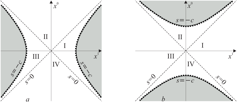
Figure 1: The Liouville metric for $\Phi>0$, $c>0$ (a) and $\Phi<0$, $c<0$ (b).

In Fig. 1, b, the allowed region of coordinates is shown for $\Phi<0$ and $c<0$. Test particles can live forever in the Universe (the rotated quadrants I or III) or fall into the black hole in quadrant II at a finite proper time, the cone $s=0$ being the horizon. This spacetime describes formation of the black hole. The spacetime in the far past is represented by the rotated quadrants I or III. There is no singularity there for $x^{0}<0$ except the white hole in quadrant IV. At a finite proper time corresponding to $s=0$ the horizon appears, and afterwards the spacelike singularity is formed.

The Liouville metric (21) can be rewritten in the Friedmann form by introduction of pseudospherical coordinates in quadrant II:

$$\begin{split}x^{0}:=&t\cosh\chi,\\ x^{1}:=&t\sinh\chi\sin\theta\cos\varphiup,\\ x^{2}:=&t\sinh\chi\sin\theta\sin\varphiup,\\ x^{3}:=&t\sinh\chi\cos\theta,\end{split}$$

where

$$t>0,\qquad\chi\in(0,\infty),\qquad\theta\in(0,\pi),\qquad\varphiup\in(0,2\pi).$$

Then the metric is

$$ds^{2}=(t^{2}+c)(dt^{2}-t^{2}d\Omega),$$ (27)

where

$$d\Omega:=d\chi^{2}+\sinh^{2}\chi(d\theta^{2}+\sin^{2}\theta d\varphiup^{2})$$

is the metric on the north sheet of two sheeted hyperboloid embedded in Minkowskian spacetime ${\mathbb{R}}^{1,3}$ (constant negative curvature three dimensional Riemannian manifold). These coordinates cover quadrant II in Fig. 1, a,b rotated in two extra space dimensions. The rotated quadrant IV is covered by the same coordinates with replacement $t\mapsto-t$.

If $\Phi>0$, we introduce new time coordinate $\tau$ defined by the differential equation

$$\frac{d\tau}{dt}=\sqrt{t^{2}+c},\qquad t^{2}+c>0$$

Then

$$\tau-\tau_{0}=\frac{t\sqrt{t^{2}+c}}{2}+\frac{c}{2}{\sf\,ln}\left|t+\sqrt{t^{2}+c}\right|,\qquad\tau_{0}=\text{const}.$$ (28)

The respective metric becomes

$$ds^{2}=d\tau^{2}-a(\tau)^{2}d\Omega,$$

and the scale factor

$$a(\tau)=t\sqrt{t^{2}+c}$$

is defined implicitly by Eq. (28). Its derivatives are

$$\begin{split}\frac{da}{d\tau}=&\frac{2t^{2}+c}{t^{2}+c},\\ \frac{d^{2}a}{d\tau^{2}}=&\frac{2ct}{(t^{2}+c)^{5/2}}.\end{split}$$ (29)

We see that the Universe in quadrant II is expanding with acceleration, constant velocity and deceleration for $c>0$, $c=0$, and $c<0$, respectively. In quadrant IV, the situation is opposite. Thus expansion with acceleration takes place for the naked singularity corresponding to $c>0$ in quadrant II. This expansion starts from the “horizon”, $t=0$, with zero scale factor, and there is no singularity in global coordinates. Going back in time, the homogeneity and isotropy of space sections are lost after crossing the “horizon” at finite proper time, and an observer turns out in the throat of the naked singularity. He sees signals from naked singularity and a hole in the center. Timelike worldlines can go through this hole and be extended to infinity. There is no big bang in this scenario.

For $\Phi<0$ and $c:=-\lambda^{2}<0$, $\lambda>0$ (otherwise the solution is not defined in quadrant II), the new coordinate $\tau$ is given by equation

$$\frac{d\tau}{dt}=\sqrt{\lambda^{2}-t^{2}},\qquad\lambda^{2}-t^{2}>0.$$

Its general solution is

$$\tau-\tau_{0}=\frac{t\sqrt{\lambda^{2}-t^{2}}}{2}+\frac{\lambda^{2}}{2}\arcsin\left(\frac{t}{\lambda}\right).$$

Now the scale factor

$$a(\tau)=t\sqrt{\lambda^{2}-t^{2}}$$

has derivatives:

$$\begin{split}\frac{da}{d\tau}=&~{}~{}\frac{\lambda^{2}-2t^{2}}{\lambda^{2}-t^{2}},\\ \frac{d^{2}a}{d\tau^{2}}=&-\frac{2\lambda^{2}t}{(\lambda^{2}-t^{2})^{5/2}}.\end{split}$$

The Universe expands for $0<t<\!\lambda/\sqrt{2}$ and contracts for $\lambda/\!\sqrt{2}<t<\lambda$ with deceleration. The scale factor is zero both on the horizon and black hole. In quadrant IV, the Universe expands for $-\lambda<t<-\lambda/\sqrt{2}$ and contracts for $-\lambda/\sqrt{2}<t<0$ with deceleration.

In quadrants I or III the solution cannot be brought to the Friedmann form because hypersurfaces $s<0$ are timelike.

Conclusion. The problem of a black hole formation has a long story started from the seminal paper [13]. Oppenheimer and Snyder assumed, in particular, that everything is spherically symmetric, the energy-momentum tensor of a star is produced by fluid-like matter, and the metric is of the Schwarzschild form outside the star. These assumptions were used in many subsequent papers. The essential point here is that the energy-momentum tensor is not obtained from the variation of matter action with respect to metric components and, in addition, there may be a problem in gluing smoothly solutions inside and outside a star. There were another approaches to matter collapse obtaining matter energy-momentum tensor from the variational principle (see, e.g. [9] and references therein). These models, to our knowledge, were solved either approximately or with strong simplifying assumptions different from ours.

In the present paper, a new simple exact global solution of Einstein equations with a scalar field is found. The solution has several novel features: 1) it is invariant under global Lorentz transformations; 2) it depends nontrivially both on time and space coordinates; 3) there are four quadratic independent involutive conservation laws for geodesics in global coordinates $x^{\alpha}$; 4) it describes, in particular, travelling through the naked singularity and the black hole formation. As far as we know, it is essentially different from all previously known solutions. For $\Phi>0$ and $c>0$, solutions describe accelerating expansion of the homogeneous and isotropic Universe under “horizon”, the scale factor there being zero. After crossing the “horizon” back in time, space sections loose their homogeneity and isotropy. This region corresponds to the throat of the naked singularity. An observer sees light rays from naked singularity, and there is the hole. Timelike worldlines can be extended through it to infinity. The obtained solutions explicitly show that cosmological solutions in General Relativity can be smoothly extended through the zero of the scale factor. This property raises the question used as the title of the paper. In addition, there is no reason to add dark energy to the model, its role is playing by the scalar field with reasonable physical properties. Hopefully, the obtained Liouville solution will help us in deeper understanding of General Relativity, black hole formation and cosmology.

Acknowledgement. The work of M.O. Katanaev was performed at the Steklov International Mathematical Center and supported by the Ministry of Science and Higher Education of the Russian Federation (agreement no. 075-15-2022-265).

References

- [1] H. Stephani, D. Kramer, M. A. H. MacCallum, C. Hoenselaers, and E. Hertl. Exact Solutions of Einstein’s Field Equations. Cambridge University Press, Cambridge, 2003.
- [2] J. B. Griffiths and Podolský. Exact Space-times in Einstein’s General Relativity. Cambridge University Press, Cambridge, 2009.
- [3] Afanasev D. E. and M. O. Katanaev. Global properties of warped solutions in general relativity with an electromagnetic field and a cosmological constant. Phys. Rev. D, 100(2):024052, 2019. https://doi.org/10.1103/PhysRevD.100.024052 http://arxiv.org/abs/arXiv:1904.04648 [physics.gen-ph].
- [4] Afanasev D. E. and M. O. Katanaev. Global properties of warped solutions in general relativity with an electromagnetic field and a cosmological constant. II. Phys. Rev. D, 101(12):124025, 2020. https://doi.org/10.1103/PhysRevD.101.124025. http://arxiv.org/abs/2006.09209 [gr-qc].
- [5] A. B. Burd and J. D. Barrow. Inflationary models with exponential potentials. Nucl. Phys., B308:929–945, 1989.
- [6] P. K. Townsend. Cosmic acceleration and M-theory. arXiv:hep-th/0308149v2 29 Aug 2003.
- [7] J. J. Halliwell. Scalar fields in cosmology with an exponental potential. Phys. Lett., B185(3-4):341–344, 1987.
- [8] A. A. Andrianov, F. Cannata, and A. Yu. Kamenshchik. General solution of scalar field cosmology with a (piecewise) exponential potential. JCAP, 10(004):19 pp., 2011.
- [9] S. Chakrabarti. Scalar field collapce with an exponential potential. Gen. Rel. Grav., 49:24(2):1–12, 2017.
- [10] L. Liouville. Mémoire sur l’intégration des équations différentielles du mouvement d’un nombre quelconque de points matériels. J. Math. Pures Appl., 14:257–299, 1849.
- [11] M. O. Katanaev. Complete separation of variables in the geodesic Hamilton-Jacobi equation. arXiv:2305.02222 [gr-qc], 2023.
- [12] M. O. Katanaev. Complete separation of variables in the geodesic Hamilton-Jacobi equation in four dimensions. Phys. Scr., 98(10):104001, 2023. DOI 10.1088/1402-4896/acf251.
- [13] J. R. Oppenheimer and H. Snyder. On continued gravitationsl contraction. Phys. Rev., 56:455–459, 1939.