Counting overlapping pairs of strings

Abstract

A correlation is a binary vector that encodes all possible positions of overlaps of two words, where an overlap for an ordered pair of words $(u,v)$ occurs if a suffix of $u$ matches a prefix of $v$. As multiple pairs can have the same correlation, it is relevant to count how many pairs of words share the same correlation depending on the alphabet size and word length $n$. We exhibit recurrences to compute the number of such pairs – which is termed population size – for any correlation; for this, we exploit a relationship between overlaps of two words and self-overlap of one word. This theorem allows us to compute the number of pairs with a longest overlap of a given length and to show that the expected length of the longest border of two words asymptotically diverges, which solves two open questions raised by Gabric in 2022. Finally, we also provide bounds for the asymptotic of the population ratio of any correlation. Given the importance of word overlaps in areas like word combinatorics, bioinformatics, and digital communication, our results may ease analyses of algorithms for string processing, code design, or genome assembly.

1 Introduction

A word $u$ overlaps a word $v$ if a suffix of $u$ equals a prefix of $v$. The shared suffix-prefix is called a border for the ordered pair of words $(u,v)$ (note that other authors call this a right border, see [5]). If $(u,v)$ has no border it is said unbordered. The pair $(u,v)$ is said mutually unbordered if both $(u,v)$ and $(v,u)$ lack a border. These notions generalize to pairs of words, the well studied notions of border, bordered and unbordered words, that were originally defined for single words.

Overlapping and unbordered words are central in many applications: bioinformatics, pattern matching, or code design. Computing overlaps between all pairs of sequencing reads is one step of the genome assembly task [8, 15]; several algorithms solve it in optimal time [9, 28, 12, 27]. The notion of borders is core in word combinatorics [14, 13], the design of pattern matching algorithms [11, 26], and in the statistical analysis of pattern finding and discovery [17, 4]. For instance, questions in vocabulary statistics deal with the distributions of the number of missing words or of common words in random texts [19, 20], which depend on the overlap structure of words, and find applications in bioinformatics [25] or in the test of random number generators [18]. Set of mutually unbordered words serve as code for synchronization purposes in network communication. A seminal construction algorithm appeared in 1973 [16], and others brought recent improvements in the design of cross bifix-free codes [2, 1], a topic of combinatorial interest [3].

Recently, Gabric gave recurrence to count bordered, mutually bordered, mutually unbordered pairs of words of length $n$ over a k-ary alphabet [5]. In his conclusion, he raised challenging open questions: 1/ count the number of pairs having a longest border of length $i$ (with $i$ satisfying $0<i<n$), and 2/ what is the expected length of the longest border of a pair of words? We address both questions in our work.

Example: Consider the binary alphabet $\{a,b\}$ and the following three words denoted by $u,v,w$: abaaa, aaabb, and abbbb. The pairs $(u,v)$ and $(v,w)$ both have a longest border of length $3$, but $(u,v)$ has $3$ distinct non empty borders aaa, aa, and a, while $(v,w)$ has only one abb.

First, this example illustrates that the possibilities of overlap of a pair $(u,v)$ depends on the self-overlapping structure of their longest border (compare aaa with abb). Second, it shows that the self overlap structure of the border limits the number of words having such a shared suffix-prefix, and thus the number of pairs of words to count. Indeed, only words of length $5$ having a suffix (resp. prefix) such as aaa or bbb, can participate in a pair having as much and as long borders as $(u,v)$. These observations suggest that to answer the open question raised by Gabric, one may have to account for the complete overlap structure of a pair of words.

Other authors have proposed to encode the starting position of such overlaps in a binary vector called a correlation [6]. In our example, the correlation of the pair $(u,v)$ is 00111, while that of $(v,w)$ is 00100. For any word $z$, the correlation of $(z,z)$ is called the autocorrelation of $z$. Clearly, multiple pairs can have the same correlation, and hence there are less correlations of length $n$ than pairs of words of length $n$.

Fortunately, one can build on earlier studies of set of autocorrelations, denoted ${\Gamma_{n}}$, and the set of correlations, denoted ${\Delta_{n}}$, for strings of length $n$ [6, 7, 22, 23]. It is known the self overlap structure of a word [6], as well as the overlap structure of a pair of words [24], does not depend on the alphabet size (provided the alphabet has at least two letters – a unary alphabet makes the question trivial). Combining a characterization of ${\Delta_{n}}$ provided in [24] and algorithm for enumerating ${\Gamma_{n}}$ [21], we can enumerate ${\Delta_{n}}$ to get the list of all correlations of length $n$.

With the terminology used in [6, 23, 20], we exhibit a solution to compute the population size of any correlation, that is the number of pairs of words having the same correlation (in Section 3). For this, we exploit a recurrence to compute the population size of autocorrelations [6]. With this in hand, we derive a formula for the abovementioned open question 1/ (Theorem 5.1), and show that expected length of longest border asymptotically diverges (open question 2/ - Theorem 5.2). Besides this, we provide bounds for the asymptotic of the population ratio of any correlation (Theorem 4.2 Section 4), which extends the result known on autocorrelations [6].

2 Preliminaries

Let $\Sigma$ be a finite alphabet, that is a set of letters of cardinality $\sigma$. We call a sequence of elements of $\Sigma$ a string or a word. The empty word is denoted by $\varepsilon$. We denote by $\Sigma^{*}$ the set of all finite strings over $\Sigma$, and by $\Sigma^{n}$ the set of all strings of length $n$ over $\Sigma$, with $n\in\mathbb{N}$. For a string $x$, $|x|$ denotes the length of $x$. For two strings $x,y$, we denote their concatenation by $xy$, and the $k$-fold concatenation of $x$ with itself by $x^{k}$ for any $k>0$. For any $L\subset{{\Sigma}^{*}}$, we define $x.L$ as $\{xy:y\in L\}$.

Let $u$ be a string of $\Sigma^{n}$. We index the letters of $u$ from $0$ to $n-1$: $u=u[0]\ldots u[n-1]$. The $i$th letter of $u$ is denoted by $u[i]$. We also denote by $u[i..j]$ for any $0\leq i\leq j<n$ the substring of $u$ starting at position $i$ and ending at position $j$. A substring is said to be proper iff $j-i+1<n$. Moreover, $u[0..j]$ is a prefix, $u[i..n-1]$ is a suffix of $u$.

2.1 Definitions of borders and correlation for pairs of strings

To study overlaps between two words, we consider ordered pairs of strings: a pair of strings $(u,v)\in\Sigma^{n}\times\Sigma^{m}$ differs from $(v,u)$, since overlaps are not symmetrical.

Definition 2.1 (Border of pair of strings).

A border of a pair of strings $(u,v)\in\Sigma^{n}\times\Sigma^{m}$ is any string that is a non-empty suffix of $u$, and a non-empty prefix of $v$. If a border exists, $(u,v)$ is said bordered, otherwise it is unbordered.

A pair may have multiple borders, and in general the set of borders for $(u,v)$ differs from that of $(v,u)$. In his article, Gabric refers to a border of $(u,v)$ as a right border and to a border of $(v,u)$ as a left border; we use a different terminology.

Guibas & Odlyzko [7] proposed to encode in a binary vector the positions in $u$ at which a border is starting, and they named this notion: a correlation of a pair of strings.

Definition 2.2 (Correlation).

Let $(u,v)\in\Sigma^{n}\times\Sigma^{m}$. The correlation of $(u,v)$, denoted $c(u,v)$, is a binary vector of length $n$ (i.e., $c(u,v)\in\{\mathtt{0},\mathtt{1}\}^{n}$) satisfying $\forall i\in[0,\dots,n-1]$

$$c(u,v)[i]=\begin{cases}\mathtt{1}&\text{ if }u[i..n-1]=v[0..i-1]\\ \mathtt{0}&\text{ otherwise.}\end{cases}$$

Generally $c(u,v)\neq c(v,u)$. A special case arises when $u$ equals $v$. Then $c(u,u)$ is called the autocorrelation of $u$ (which encodes the set of periods of $u$) [7], which for clarity, we will denote by $a(u)$. To each border $z$ of a word $u$ is associated a period, which is an integer equal to $|u|-|z|$. For the sake of simplicity, in this work, we focus on pairs of strings of equal length, that is, when $m=n$.

Example 2.3.

Consider the pair of strings $(u,v)=(aabbaa,baabaa)$ of length $6$ over the binary alphabet $\{a,b\}$. The pair $(u,v)$ has a border starting at position $3$ in $u$, and a shorter border starting at position $5$. Its correlation is $c(u,v)=\mathtt{000101}$. See Table 1. Of course, a permutation of the alphabet (that is exchanging $a$ with $b$ and vice versa) yields a different pair of strings, which has the same correlation as $(u,v)$. Thus, several pairs can share the same correlation.

pos.	0	1	2	3	4	5	6	7	8	9	10
$u$	a	a	b	b	a	b	-	-	-	-	-	$t$
$v$	b	a	b	b	a	a	-	-	-	-		0
	-	b	a	b	b	a	a	-	-	-	-	0
	-	-	b	a	b	b	a	a	-	-	-	0
	-	-	-	b	a	b	b	a	a	-	-	1
	-	-	-	-	b	a	a	b	a	b	-	0
	-	-	-	-	-	b	a	b	b	a	a	1

Table 1: Example of correlation for the pair $(u,v):=(aabbab,babbaa)$ of length $6$. All possible shifts of $v$ to the right of $u$ are displayed on distinct lines: those at which an overlap exists are colored in blue. The last column shows $c(u,v)$ written top-down, with $\mathtt{1}$ bits corresponding to borders also colored in blue.

We recall some known properties of autocorrelations that we use later on. Their proofs can be found in [24, 6, 10].

Lemma 2.4.

Let $t\in{\Gamma_{n}}$ and $u\in{{\Sigma}^{n}}$ such that $a(u)=t$. Let $0\leq p\leq q<n$ such that $t[p]=\mathtt{1}$. Then, $t[q]=\mathtt{1}$ iff $u[p..n-1]$ has period $(q-p)$ (equivalently the $(q-p)$ bit in $a(u[p..n-1])$ equals $\mathtt{1}$).

Lemma 2.5.

Let $t\in\Gamma_{n}$. For all $p$ satisfying $0\leq p<n$, and $t[p]=1$, it follows that $t[kp]=1$ for all $k\in[2,\dots,\lfloor{\frac{n}{p}}\rfloor].$

Lemma 2.6.

Let $\pi(u)$ be the basic period (the minimum non-trivial period) of $u\in\Sigma^{n}$, and $p$ be a non-trivial period. Then either $p=k\cdot\pi(u)$, $k\in[1,\dots,\lfloor{\frac{n}{\pi(u)}}\rfloor]$ or $p>n-\pi(u)$.

2.2 Set of all correlations of length $n$ and its characterization

As in [23], for any length $n\in\mathbb{N}$, we denote the set of all correlations for words of length $n$ by $\Delta_{n}$ and its cardinality by $\delta_{n}$. The set of all autocorrelations of strings of length $n$ is denoted by $\Gamma_{n}$ and its cardinality by $\kappa_{n}$. When $n=0$ we consider that $\delta_{n}={\Gamma_{n}}=\{\varepsilon\}$. So $\Delta_{n}:=\{t\in\{\mathtt{0,1}\}^{n}:\exists(u,v)\in{{\Sigma}^{n}}\times{{\Sigma}^{n}}:c(u,v)=t\}$ and $\Gamma_{n}:=\{s\in\{\mathtt{0,1}\}^{n}:\exists u\in{{\Sigma}^{n}}:a(u)=s\}$.

The first characterization of autocorrelation was given by Guibas and Odlyzko in their seminal paper [6]. They studied the cardinality of ${\Gamma_{n}}$ and provided a lower and an upper bound for $\log({\kappa_{n}})/\log_{2}(n)$, and conjectured that their lower bound was also an upper bound. They also proposed an algorithm to compute the number of strings in ${{\Sigma}^{n}}$ that share the same period set, which they termed the population of an autocorrelation. A key result of their work is the alphabet independence of ${\Gamma_{n}}$: Any alphabet with $\sigma>1$ gives rise to the same set of autocorrelations, i.e., to ${\Gamma_{n}}$.

Rivals et al. [24] have characterized $\Delta_{n}$ and exhibited its relation to the sets $\Gamma_{j}$ for $0\leq j\leq n$, which is stated below.

Lemma 2.7 (Lemma 21 [24] ).

The set of correlations of length $n$ is of the form

$$\Delta_{n}=\left\{0^{(n-j)}s,\;\text{ with }s\in\Gamma_{j}\;\text{ and }\ j\in[0,\dots,n]\right\}.$$

Lemma 2.7 gives us the structure of any correlation for any pair of strings $(u,v)$ of length $n$: it starts with a series of $0$, until the leftmost $1$, which marks the position in $u$ of the longest border of pair $(u,v)$. Let $z$ denote this border and $j$ denote its length. The above characterization is based on the fact that the suffix of length $j$ of $c(u,v)$ (the one starting with the leftmost $1$) must be the autocorrelation of $z$. Indeed, each border of $z$ is also a border of $(u,v)$. If $j=0$, then $z$ is empty string and $c(u,v)=0^{n}$. Of course, if $u=v$, then the correlation of $(u,v)$ is the autocorrelation of $u$.

A reformulation of this explanation is stated in the following corollary. We will often use this statement later on in this article.

Corollary 2.8.

Let $n>0$ and $t\in{\Delta_{n}}$. Then there exist $j\in[0,n]$ and $s\in\Gamma_{j}$ such that $t=0^{(n-j)}s$.

This characterization implies the following partition of $\Delta_{n}$:

Corollary 2.9.

$\Delta_{n}=\bigcup_{j=0}^{n}\{\mathtt{0}^{n-j}s\,|\,s\in\Gamma_{j}\}=\bigcup_{j=0}^{n}\left(\mathtt{0}^{n-j}.\Gamma_{j}\right)$.

Since correlations (and autocorrelations) are binary encoding of a set of positions, we can get the intersection (or union) of two correlations by taking their logical AND (or OR). For legibility, for $t,t^{\prime}\in\Delta_{n}$ we denote their intersection by $t\cap t^{\prime}$ and their union by $t\cup t^{\prime}$ . We use such notation to investigate the algebraic structure of $\Delta_{n}$ in Appendix A.

Rivals et al. [24] studied the cardinalities of $\Gamma_{n}$ and $\Delta_{n}$, and proved the asymptotic convergence of ratios involving $\kappa_{n}$ and $\delta_{n}$ towards the same limit when $n$ tends to infinity. Precisely, $\frac{\ln\delta_{n}}{\ln^{2}(n)}\rightarrow\frac{1}{2\ln(2)}$ when $n\rightarrow\infty$.

It is interesting to study the algebraic structure of ${\Delta_{n}}$. In Appendix A, we show that $\Delta_{n}$ is a lattice under set inclusion, and that it does not satisfy the Jordan-Dedekind condition. The example 2.10 and Figure 1 illustrate the lattice structure of ${\Delta_{n}}$ for $n=4$.

Example 2.10.

Figure 1 illustrates the lattice structure with $\Delta_{4}$, for strings of length $n=4$. From Corollary 2.9, one has $\Delta_{4}=\Gamma_{4}\cup(\mathtt{0}.\Gamma_{3})\cup(\mathtt{00}.\Gamma_{2})\cup(\mathtt{000}.\Gamma_{1})\cup\{\mathtt{0000}\}$.

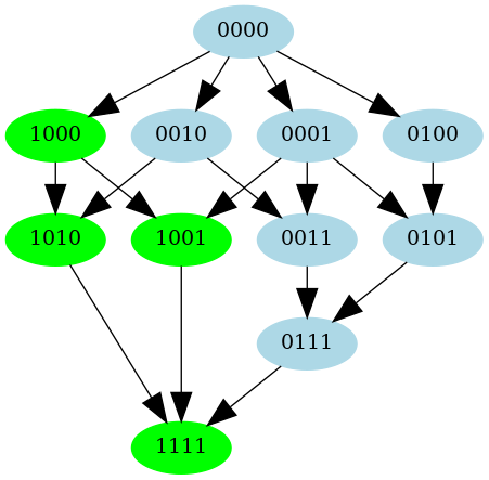
Figure 1: The lattice of $\Delta_{4}$: each node contains a correlation as a binary vector. The elements of $\Gamma_{4}$ are colored in green. Since between 0000 and 1111 there are chains of different lengths ($3$ and $4$), $\Delta_{4}$ does not satisfy the Jordan-Dedekind condition.

Table 2: Pair population sizes on a binary alphabet for correlations of $\Delta_{4}$; $\sigma=2$ and $n=4$.

correlation	pair
	population
	size
0000	74
0001	82
0010	30
0011	24
0100	16
0101	8
0111	6
1000	6
1001	6
1010	2
1111	2

3 Population size of a correlation

The population of a correlation $t\in{\Delta_{n}}$ is defined as: $POP(t):=\{(u,v)\in{{\Sigma}^{n}}\times{{\Sigma}^{n}}\text{ such that }\\ c(u,v)=t\}$. We want to compute its cardinality, i.e. the population size, which we denote by $pop(t)$. For example, consider the correlation $t:=01010$ from $\Delta_{5}$: over the alphabet $\Sigma=\{a,b\}$, we have $POP(t)=\{(ababa,babaa),(ababa,babab),(bbaba,babab),(bbaba,babaa),\\ (aabab,ababa),(aabab,ababb),(babab,ababa),(babab,ababb)\}$ and $pop(t)=8$.

Let us give an overview of our results and detail how they generalize or improve existing ones. First, for a given autocorrelation $t\in{\Gamma_{n}}$ there exists a linear time realization algorithm to build a binary string $u$ such that $a(u)=t$ [21]. We will exhibit such a realization algorithm for any correlation $t\in{\Delta_{n}}$ in Section 3.1. In fact, this is related to counting not the pairs of $POP(t)$, but single strings either $u$ or $v$, for which such pair exist. We show a formula to determine the cardinality of $POP_{l}(t):=\{u\in{{\Sigma}^{n}}:\exists v\in{{\Sigma}^{n}}\text{ such that }c(u,v)=t\}$ or of $POP_{r}(t):=\{v\in{{\Sigma}^{n}}:\exists u\in{{\Sigma}^{n}}\text{ such that }c(u,v)=t\}$. Note that as $u$ and $v$ play a symmetrical role in $POP_{l}(t)$ and $POP_{r}(t)$, it implies that their cardinalities, denoted $pop_{r}(t)$ and $pop_{l}(t)$, must be equal. Clearly, $pop^{2}_{r}(t)$ is an upper bound for $pop(t)$.

Second, there exist, two algorithms for computing the population size of an autocorrelation (i.e., when $t=a(u)$). A recurrence formula for the population size of an autocorrelation was proposed in [6][Theorem 7.1] and with it the authors investigated the asymptotics of the population size (Theorem 7.2). Another algorithm takes advantage of the fact that ${\Gamma_{n}}$, the set of autocorrelations of length $n$, forms a lattice with set inclusion [23]. We will review the recurrence formula from [6] (see page 3.2) and use it to propose one for correlations (Theorem 3.10 in Section 3.2). Another recurrence is proven in Theorem C.1 in Appendix C.

3.1 Computing the single population size

First, we need a simple Lemma about occurrences of a suffix of a word.

Lemma 3.1.

Let $i>0$ and $j>0$ be two integers. Let $u\in\Gamma_{i}$ and $v\in\Gamma_{j}$. If the first letter of $v$ does not occur in $u$, then $v$ occurs in $uv$ only at position $i$.

Let now us state the realization problem and describe our binary realization algorithm. Problem: Consider the binary alphabet $\Sigma=\{a,b\}$. Let $n>0$ and let $t\in{\Delta_{n}}$. Find a pair $(u,v)$ of strings over $\Sigma$, such that $c(u,v)=t$.
Algorithm: If $t[0]=\mathtt{1}$, then $t$ is an autocorrelation. Then, call the binary realization algorithm for autocorrelation with input $t$ and return the obtained binary word [21]. If $t=\mathtt{0}^{n}$, the pair of strings shall not overlap at all. Thus $u:=a^{n}$ and $v:=b^{n}$ satisfy the correlation vector $t$. Otherwise, we know there exists $0<j<n$ and $s\in\Gamma_{j}$ such that $t=\mathtt{0}^{n-j}s$. This is the main case.
Call the binary realization algorithm for autocorrelation with $s$ as input, and denote by $w$ the returned binary word. $w$ has length $j$ and must be the suffix of $u$ and prefix of $v$. Without loss of generality, assume $w[0]=a$. Then, setting $u:=b^{n-j}w$, and taking any $v$ in the set $w.\Sigma^{(n-j)}$, we get

• $w$ is border of $(u,v)$, and thus $s$ is a suffix of $c(u,v)$;

• $w$ has only one occurrence in $u$ by Lemma 3.1, and is thus the longest border of $(u,v)$.

Hence, we get $c(u,v)=\mathtt{0}^{n-j}s$ as required. Finally, return $(u,v)$ with $v:=w.a^{n-j}$.

From this realization algorithm, in the main case, we see that for a fixed $t\in\Delta_{n}$, once $w$ and $u$ are chosen as above, there exist $\sigma^{(n-j)}$ pairs since $v$ can be any word in $w.\Sigma^{(n-j)}$. This is a maximum for $pop_{r}(t)$ once $w$ is fixed. Hence, we obtain the following Lemma to compute the single population size. A formal proof appears in Appendix B.

Lemma 3.2.

Let $t:=\mathtt{0}^{n-j}s$ be in ${\Delta_{n}}$ with $j\in[1,\dots,n]$. Then the single population size of $t$ satisfies: $pop_{r}(t)=pop(s)\cdot\sigma^{(n-j)}$.

Remark: if $j=0$, then the pair of strings $(u,v)$ is unbordered. Note that if $vu\in\Gamma_{2n}$ with $|u|=|v|=n$ and is unbordered, then $(u,v)$ is also unbordered. Therefore, all such pairs of strings (aka "bifix-free sequences") can be constructed by the algorithm of Nielsen [16].

3.2 Computing the pair population size

Before, finding a formula to compute $pop(t)$, i.e. the pair population size, of a correlation $t$ in ${\Delta_{n}}$, we show that $pop(t)$ is related to the population size of some autocorrelations of strings of length $2n$ in Theorem 3.7. To achieve this, we demonstrate two lemmas linking the borders of a pair $(u,v)$ with the borders of the string $vu$.

Lemma 3.3.

Let $t\in{\Delta_{n}}$ and let $(u,v)\in\Sigma^{n}\times\Sigma^{n}$ such that $c(u,v)=t$. Then, $t$ is the suffix of length $n$ of the autocorrelation of the word $vu$.

Proof 3.4.

Let $t\in{\Delta_{n}}$ and $(u,v)$ be a pair of words as in the lemma. By Lemma 2.7, we know there exists $j\in[0,\dots,n]$ and $s\in\Gamma_{j}$ such that $t=0^{(n-j)}s$. If we denote by $z$ the longest border of $(u,v)$, then $|z|=j$. We distinguish two cases depending on $j$.

Case 1. If $j=n$ then $u=v=z$, $t=s=a(u)$ and $vu=uu$. As the word $uu$ has period $|u|$, then by Lemma 2.4, then $t$ is the suffix of length $n$ of $a(vu)$.

Case 2. Otherwise $j<n$. By hypothesis, there exist two words $x$ and $y$ of length $n-j$ such that $u=xz$ and $v=zy$. Hence, $vu=zyxz$ and $z$ is a border of $vu$. As $|zyx|=2n-j$, it implies that $vu$ has period $2n-j$, and by Lemma 2.4 $s$ is the suffix of length $j$ of $a(vu)$.
Let us show by contraposition that for any position $n\leq i<2n-j$ the i-th bit of $a(vu)$ is 0. Let $i$ be a integer such that $n\leq i<2n-j$ and assume the the i-th bit of $a(vu)$ equals 1. Then, $vu$ would have a border of length $2n-i$ with $n\geq 2n-i>j$, and this border would also be a border of $(u,v)$, which contradicts the maximality of $z$. Hence, $t$ is a suffix of $a(vu)$.

Lemma 3.5.

Let $w\in\Sigma^{2n}$; let $u$ and $v$ be words in ${{\Sigma}^{n}}$ such that $w=vu$. If $w$ has a border, then the pair of strings $(u,v)$ is bordered.

Proof 3.6.

Let $w$, $u$, and $v$ be as in the lemma. If $u=v$, then $u$ is a border of the pair $(u,u)$. Otherwise, we have $u\neq v$. Let $z$ be a border of $w$. We distinguish two cases based on $|z|$.

1. Case 1: $|z|\in[1,\dots,n-1]$. Then, there exist two words $x,y$ of length $n-|z|$ such that $v=zy$ and $u=xz$. Thus, $z$ is a border of $(u,v)$.

2. Case 2: $|z|\in[n+1,\dots,2n-1]$. Then, $w$ has a period $p:=2n-|z|$ and $p<n$ (the half $|w|$). According to properties of periods (Lemma 2.5), the integer $\lfloor{\frac{2n}{p}}\rfloor p$ is also period of $w$. Then, if we denote its corresponding border by $z^{\prime}$, we have $|z^{\prime}|<n$, and we are back to case 1, with $z^{\prime}$ being a border of $(u,v)$.

Before stating the theorem on the population size of a correlation, we need a notation. Let $t\in{\Delta_{n}}$. We denote by $G(t)$ the set of all strings of length $2n$ whose autocorrelation has $t$ as suffix, and by $g(t)$ the cardinality of $G(t)$. Formally, $G(t):=\{w\in\Sigma^{2n}:t\text{ is a suffix of }a(w)\}$.

The following theorem shows the relation between the number of pairs of strings of length $n$ and the number of specific strings of length $2n$. For $t\in\Gamma_{n}$, $pop(t)$ can be directly calculated using Theorem 3.9. Therefore we consider $t\in\Delta_{n}$ but exclude those in $\Gamma_{n}$.

Theorem 3.7.

Let $t\in\Delta_{n}\setminus\Gamma_{n}$. Then, $pop(t)=g(t)$.

Proof 3.8.

i/ Let us first prove that $pop(t)\leq g(t)$. Let $(u,v)\in POP(t)$. According to Lemma 3.3, the string $vu$ belongs to $G(t)$. This implies that $pop(t)\leq g(t)$.
ii/ Let us prove that $pop(t)\geq g(t)$. Let $w\in G(t)$, and let $u$ and $v$ be strings of length $n$ such that $w=vu$. As $t\in{\Delta_{n}}$, by Lemma 2.7, we know there exists $j\in[0,\dots,n]$ and $s\in\Gamma_{j}$ such that $t=0^{(n-j)}s$.

If $j=0$, then $t=0^{n}$. We show that $a(w)=\mathtt{1}\mathtt{0}^{2n-1}$. Indeed, assume $w$ has a period smaller than $n$, then by Lemma 2.5 it would also have periods $>n$, which contradicts $t=0^{n}$. Thus, $c(u,v)=t$ and $(u,v)$ belongs to $POP(t)$.

If $0<j<n$. Then $w[0..j-1]$ is the longest border of $w$ with length $j<n$. From Lemma 3.5 (specifically, case 1), we get that $(u,v)$ belongs to $POP(t)$. In both cases, this implies that $g(t)\leq pop(t)$.

Combining both inequalities, we get $pop(t)=g(t)$, which concludes the proof.

Now we will calculate the number of pairs of strings of length $n$ with the correlation $t=0^{n-j}s\in\Delta_{n}$ where $s\in\Gamma_{j}$, i.e., the population size of $t$. Our result is based on the recurrence for the population size of autocorrelation by Guibas & Odlyzko [6], as well as our Theorem 3.7.

We review the recurrence formula given by Guibas & Odlyzko. Let $s\in\Gamma_{j}$. They define the autocorrelation of length $n$ denoted as $s_{n}:=10^{n-j-1}s$, and the sequence $\psi$ for $k\in\mathbb{N}$ depending on $s_{k}$ and $s$ as

$$\psi[k]:=\begin{cases}0&\text{for }k>j\\ s[j-k]&\text{for }1\leq k\leq j\\ \sigma^{-k}&\text{for }k<1.\end{cases}$$

The sequence $\psi$ partitions $\mathbb{N}$ into three distinct ranges. For $k<1$, $\psi[k]$ equals $\sigma^{-k}$. In the interval $1\leq k\leq j$, $\psi[k]$ equals $1$ if $(j-k)$ is a period of $s$, and $0$ otherwise. For any $k>j$, $\psi[k]$ is consistently equal to $0$. Theorem 3.9 states their recurrence for $pop(s_{n})$.

Theorem 3.9 (Population size of an autocorrelation (Theorem 7.1 [6]) ).

The number of strings of length $n$ which have autocorrelation $s_{n}$ satisfies the recurrence

$$pop(s_{n})+\sum_{k}pop(s_{k})\psi[2k-n]=2\psi[2j-n]pop(s),$$

where $pop(s_{k})=0$ for $k<j$.

We state our result regarding the population size of a correlation $t=0^{n-j}s$ with $s$ being fixed. See Table 2 for pair population sizes on a binary alphabet for all correlations in $\Delta_{4}$. Note that if $j=n$, then the population size of $t$ is the known population size of $s$.

Theorem 3.10 (Population size of a correlation (I)).

Let $\lambda,j,n\in\mathbb{N}$ satisfying $0\leq\lambda,j<n$. Let $t:=0^{n-j}s$ be an element of $\Delta_{n}$ with $s\in\Gamma_{j}$. Then the population size of $t$ satisfies the recurrence

$$pop(t)=\sum_{\lambda=\lceil\frac{2n-j}{2}\rceil}^{n-1}pop(s_{(2n-\lambda)})\cdot s[j+2\lambda-2n]+pop(s_{2n}).$$

Proof 3.11.

Let $w\in G(t)$ and define the integer $\lambda$ as $\lambda:=\max\{0\leq i<n:a(w)[i]=\mathtt{1}\}$. According to Theorem 3.7, we know that $pop(t)=g(t)$. Thus we are left to show

$$g(t)=\sum_{\lambda=\lceil\frac{2n-j}{2}\rceil}^{n-1}pop(s_{(2n-\lambda)})\cdot s[j+2\lambda-2n]+pop(s_{2n}).$$

Define $s_{(2n,\lambda)}:=*^{\lambda}\mathtt{1}\mathtt{0}^{2n-\lambda-j-1}s\in\{0,1\}^{2n}$, where $*$ is a doesn’t care symbol in {0,1}. Note that this defines a binary vector of length $2n$, which may belong to $\Gamma_{2n}$ depending on the value of $\lambda$. Let us partition the set $G(t)$ into its subsets $POP(s_{(2n,\lambda)})$, where $s_{(2n,\lambda)}\in\Gamma_{2n}$

$$G(t)=\bigsqcup_{\lambda\in[0,\dots,n-1]:s_{(2n,\lambda)}\in\Gamma_{2n}}POP(s_{(2n,\lambda)}).$$

Taking the cardinalities, for $s_{(2n,\lambda)}\in\Gamma_{2n}$ we get

$$g(t)=\sum^{n-1}_{\lambda=0}pop(s_{(2n,\lambda)})=\sum^{n-1}_{\lambda=1}pop(s_{(2n,\lambda)})+pop(s_{(2n,0)}).$$

We distinguish different cases depending on $\lambda$.

1. When $\lambda=0$. The autocorrelation of $w$ satisfies $a(w)=s_{(2n,0)}=s_{2n}=10^{2n-j-1}s\in\Gamma_{2n}$. Thus the number of strings $w$ having the autocorrelation $s_{(2n,0)}$ equals the population size of $s_{2n}$, i.e., $pop(s_{(2n,0)})=pop(s_{2n})$.

2. When $\lambda\in[1,\dots,n-1]$. Recall $s_{(2n-\lambda)}=\mathtt{1}\mathtt{0}^{2n-\lambda-j-1}s$, then we have $s_{(2n,\lambda)}=*^{\lambda}s_{(2n-\lambda)}\in\{0,1\}^{2n}$. Note that not all $s_{(2n,\lambda)}$ belongs to $\Gamma_{2n}$, but all $a(w)$ must have the form $s_{(2n,\lambda)}$. We will identify all elements $a(w)$ in $\Gamma_{2n}$ that take the form $s_{(2n,\lambda)}$. By the definition of $\lambda$, we know $\lambda<|w|/2$ which indicates at most one $a(w)$ can possibly exist by given $s_{(2n-\lambda)}$. Note that $a(w)[2\lambda]=1$ where $2\lambda\in[2n-j,\dots,2n-2]$, this implies $\lambda\geq\lceil(2n-j)/2\rceil$. Denote by $\pi(w)$ the basic period of $w$, then $a(w)$ could be decomposed as $a(w)=(10^{\pi(w)-1})^{\alpha}s_{(2n-\lambda)}$ where $\alpha=\lambda/\pi(w)$ by Lemma 2.6. By Lemma 2.4, such an $a(w)$ exists precisely if $s[2\lambda-(2n-j)]=s[j+2\lambda-2n]=1$ since $a(w)[2n-j]=1$ and $j+2\lambda-2n\in[0,\dots,j-1]$. Thus we have

   $$\sum^{n-1}_{\lambda=1}pop(s_{(2n,\lambda)})=\sum_{\lambda=\lceil\frac{2n-j}{2}\rceil}^{n-1}pop(s_{(2n-\lambda)})s[j+2\lambda-2n].$$

Combine the two cases, we get $pop(t)=\sum_{\lambda=\lceil\frac{2n-j}{2}\rceil}^{n-1}pop(s_{(2n-\lambda)})\cdot s[j+2\lambda-2n]+pop(s_{2n})$.

Observe that in Theorem 3.10, calculating the population size of $t=0^{n-j}s$ requires to compute $pop(s_{(2n-\lambda)})$ for all $\lambda\in[\lceil\frac{2n-j}{2}\rceil,\dots,n-1]\cup\{0\}$ by Theorem 3.9. Therefore, we provide another recurrence on $t$ which calculates $pop(t)$ relying only on $s$. See details in Appendix C.1.

4 Asymptotics on the population ratios

The population ratio of a correlation $t\in{\Delta_{n}}$ is $pop(t)/\sigma^{2n}$. Here, we study the asymptotic lower and upper bounds for this ratio. Before stating our result, we give several definitions introduced by Guibas & Odlyzko [6]. Recall that Theorem 3.9 on the population size of an autocorrelation $s_{n}$ relies on a sequence $\psi[k]$. They define three generating functions (with dummy variable $z$) two for $pop(s_{n})$ and $\psi[k]$, and introduce $\widetilde{pop}(z)$, which is the normalization of ${pop}(z)$ by ${pop}(s)$. Their definitions are as follows:

$$pop(z)=\sum_{n=0}^{\infty}pop(s_{n})z^{-n};\quad\psi(z)=\sum_{n=0}^{\infty}\psi[k]z^{-n};\quad\widetilde{pop}(z)=\frac{pop(z)}{pop(s)}.$$

Thus Theorem 3.9 can be rewritten as:

$$\widetilde{pop}(z)+\psi(z)\widetilde{pop}(z^{2})=2\psi(z)z^{-2j}.$$ (1)

Hence, the asymptotics of $pop(s_{n})$ as $n\rightarrow\infty$ with $s$ being fixed follows.

Theorem 4.1 (Asymptotics on the population sizes (Theorem 7.2 [6])).

Let $\mu$ be any small positive complex number. The population size of $s_{n}$ divided by the population size of $s$ over an alphabet of cardinality $\sigma\geq 2$ satisfies

$$\frac{pop(s_{n})}{pop(s)}=\left(\frac{2}{\sigma^{2j}}-\widetilde{pop}(\sigma^{2})\right)\sigma^{n}+O((\sigma+\mu)^{\frac{n}{2}}),$$

where $\widetilde{pop}(\sigma^{2})$ satisfies the Functional Equation (1).

Denote $c=\frac{2}{\sigma^{2j}}-\widetilde{pop}(\sigma^{2})$. Note that $c$ is the asymptotic limit of $pop(s_{n})/(pop(s)\sigma^{n})$; thus $c\cdot pop(s)$ provides the limiting value of $pop(s_{n})/\sigma^{n}$. Here we state our result on the population size of $t$ with $s$ being assumed fixed. See Table 3 for some interesting cases on the limiting values of $pop(s_{n})/\sigma^{n}$ and asymptotic bounds on $pop(t)/\sigma^{2n}$.

Theorem 4.2 (Asymptotics on the population ratios).

Let $\mu$ be any small positive complex number. Let $t:=0^{n-j}s\in{\Delta_{n}}$ with $j\in[0,\dots,n-1]$. Over an alphabet of cardinality $\sigma\geq 2$, the ratio $pop(t)/pop(s)$ satisfies the asymptotic inequality:

$$c\cdot\sigma^{2n}+O((\sigma+\mu)^{n})\leq\frac{pop(t)}{pop(s)}<\frac{c\cdot\sigma}{\sigma-1}\cdot\sigma^{2n}+O(n(\sigma+\mu)^{n}).$$ (2)

In particular, we have the asymptotic bounds on the population ratio $pop(t)/\sigma^{2n}$

$$c\cdot pop(s)\leq\lim_{n\rightarrow\infty}\frac{pop(t)}{\sigma^{2n}}<\frac{c\cdot\sigma}{\sigma-1}\cdot pop(s).$$ (3)

Proof 4.3.

By Theorem 3.10 on the population size of $t$, for $\lambda\in[\lceil\frac{2n-j}{2}\rceil,\dots,n-1]\cup\{0\}$, we have.

$$\frac{pop(t)}{pop(s)}=\frac{\sum_{\lambda}pop(s_{(2n-\lambda)})\cdot s[j+2\lambda-2n]+pop(s_{2n})}{pop(s)}.$$ (4)

Then (4) could be bounded above and below by:

$$\frac{pop(s_{2n})}{pop(s)}\leq\frac{\sum_{\lambda}pop(s_{(2n-\lambda)})\cdot s[j+2\lambda-2n]+pop(s_{2n})}{pop(s)}<\frac{\sum_{\lambda=0}^{n}pop(s_{(2n-\lambda)})}{pop(s)}.$$ (5)

From Theorem 4.1, for any $\lambda\in[0,\dots,n]$ we have:

$$\frac{pop(s_{(2n-\lambda)})}{pop(s)}=c\cdot\sigma^{2n-\lambda}+O((\sigma+\mu)^{\frac{2n-\lambda}{2}}).$$ (6)

Plugging in (6) in the left hand side of (5) we get

$$\frac{pop(s_{2n})}{pop(s)}=c\cdot\sigma^{2n}+O((\sigma+\mu)^{n})$$

and in the right hand side of (5) we obtain:

$$\sum_{\lambda=0}^{n}\frac{pop(s_{(2n-\lambda)})}{pop(s)} = c\cdot\sum_{i=n}^{2n}\sigma^{i}+\left(O((\sigma+\mu)^{n})+O((\sigma+\mu)^{\frac{2n-1}{2}})+\dots+O((\sigma+\mu)^{\frac{n}{2}})\right)$$

$$= \frac{c\sigma}{\sigma-1}\cdot\sigma^{2n}+O(n(\sigma+\mu)^{n})$$

Combining both equations, we obtain (2):

$$c\cdot\sigma^{2n}+O((\sigma+\mu)^{n})\leq\frac{pop(t)}{pop(s)}<\frac{c\cdot\sigma}{\sigma-1}\cdot\sigma^{2n}+O(n(\sigma+\mu)^{n}).$$

Multiplying (2) by $pop(s)/\sigma^{2n}$, we get the desired bounds (3) on the asymptotic behavior of the population ratio $pop(t)/\sigma^{2n}$.

Table 3: For $\sigma=2,3$ and $24$, we give the limiting values of $pop(s_{n})/\sigma^{n}$ (column 3) and asymptotic bounds on $pop(t)/\sigma^{2n}$ (column 4) for some autocorrelations $s$. The limiting values of $pop(s_{n})/\sigma^{n}$ in column 3 are taken from [6]. Note that the lower bound in column 4 coincides with the value in column 3 (for a given $s$ and $\sigma$). The correlations $\varepsilon$ and $0^{n-1}1$ are the most "popular" for $\sigma=2$, but it is not possible to distinguish which one is the most popular. It differs from the autocorrelation case, where $10^{n-2}1$ is the most popular. For $\sigma\geq 3$, the trivial correlation is the most popular, as in the autocorrelation case.

Alphabet Size $\sigma$	Autocorrelation $s$	$pop(s_{n})/\sigma^{n}$	$pop(t)/\sigma^{2n}$
2	$\varepsilon$	0.268	[0.268, 0.536)
	1	0.300	[0.300, 0.600)
	10	0.110	[0.110, 0.220)
	11	0.089	[0.089, 0.178)
3	$\varepsilon$	0.557	[0.557, 0.836)
	1	0.283	[0.283, 0.424)
	10	0.072	[0.072, 0.108)
	11	0.032	[0.032, 0.048)
24	$\varepsilon$	0.957	[0.957, 0.999)
	1	0.042	[0.042, 0.044)

5 Solutions to Gabric’s open questions

In the article about bordered and unbordered pairs of words [5], the author raises two challenging open questions: 1/ How many pairs of length-$n$ words have a longest border of fixed length $j$? and 2/ what is the expected length of the longest border of a pair of words?. Note that with his terminology, a border is either a right-border or a left-border depending on the order of words in the pair. As the words play symmetrical roles in the definition of border, the counts for question 1/ are equal.

From the characterization of the set of correlations (Lemma 2.7), we know that correlations are partitioned by their longest border (Corollary 2.9). To consider pairs with longest border of length say $j$, we must count pairs having a correlation $t$ in the subset $(\mathtt{0}^{n-j}.\Gamma_{j})$ of ${\Delta_{n}}$. With the recurrence that computes the population size for any correlation $t$ (Theorem 3.10), it suffices to sum up $pop(t)$ over all $t$ in this subset to answer question 1/, which yields Corollary 5.1.

For question 2/, we take the average over this same subset as shown below in the equation of $E(X)$ on page 5.2. This provides a general formula and allows us to investigate the limit of this expectation, and to show in Theorem 5.2 that it diverges when the string length $n$ tends to infinity.

5.1 Counting pairs of strings with a longest border of fixed length

Corollary 5.1.

Let $L_{j}$ be the number of pairs of strings of length $n$ that have a longest border of length $j$. Let $s$ be any autocorrelation of $\Gamma_{j}$. Let $t:=0^{n-j}s\in(\mathtt{0^{n-j}}.\Gamma_{j})$. Let $s_{(2n-\lambda)}=10^{2n-\lambda-j-1}s\in\Gamma_{(2n-\lambda)}$ where $\lambda\in[\lceil\frac{2n-j}{2}\rceil,\dots,n-1]\cup\{0\}$. Then

$$L_{j}=\sum_{t\in(\mathtt{0}^{n-j}.\Gamma_{j})}pop(t)=\sum_{\lambda=\lceil\frac{2n-j}{2}\rceil}^{n-1}\sum_{s\in\Gamma_{j}}pop(s_{(2n-\lambda)})\cdot s[j+2\lambda-2n]+\sum_{s\in\Gamma_{j}}pop(s_{2n}).$$

5.2 Expected value of the longest border of a pair of words

In [5], Gabric considers a fixed alphabet size $\sigma$ and a Bernoulli i.i.d model for random words. In this model, the probability that a character occurs at any position is independent of other positions and equals $1/\sigma$. For a fixed word length $n$, the probability of any pair of words $(u,v)$ both of length $n$ is $1/\sigma^{2n}$. Gabric shows that, for the expected length of the shortest border of a pair of words converges to a constant. In contrast, we show that the asymptotic expected length of the longest border actually diverges.

Define $X$ to be the length of the longest border of a pair of strings $(u,v)$. Then, the expectation of $X$ is

$$E(X)=\sum_{j=0}^{n-1}j\cdot Pr(X=j)=\sum_{j=1}^{n-1}j\cdot\frac{L_{j}}{\sigma^{2n}}=\sum_{j=1}^{n-1}j\cdot\frac{\sum_{t\in(\mathtt{0^{n-j}}.\Gamma_{j})}pop(t)}{\sigma^{2n}}.$$

Theorem 5.2.

The asymptotic expected length of the longest border of a pair of strings $(u,v)$ diverges.

Proof 5.3.

The asymptotic expected length of the longest border of $(u,v)$ is:

$$E_{\infty}(X)=\lim_{n\rightarrow\infty}\sum_{j=1}^{n-1}j\cdot\frac{\sum_{t\in(\mathtt{0^{n-j}}.\Gamma_{j})}pop(t)}{\sigma^{2n}}.$$

We claim that $\sum_{t\in(\mathtt{0^{n-j}}.\Gamma_{j})}pop(t)/\sigma^{2n}\geq c$ when $n\rightarrow\infty$, where $c$ is a positive constant as defined in Section 4. To see this, note that $\sum_{t\in(\mathtt{0^{n-j}}.\Gamma_{j})}pop(t)/\sigma^{2n}$ satisfies the following equation by Corollary 5.1.

$$\frac{\sum_{t\in(\mathtt{0^{n-j}}.\Gamma_{j})}pop(t)}{\sigma^{2n}} =\frac{\sum_{\lambda=\lceil\frac{2n-j}{2}\rceil}^{n-1}\sum_{s\in\Gamma_{j}}pop(s_{(2n-\lambda)})\cdot s[j+2\lambda-2n]+\sum_{s\in\Gamma_{j}}pop(s_{2n})}{\sigma^{2n}}$$

$$\geq\frac{\sum_{s\in\Gamma_{j}}pop(s_{2n})}{\sigma^{2n}}.$$ (7)

By Theorem 3.9 and since $\sum_{s\in\Gamma_{j}}pop(s_{2n})\geq 1$, the right side of (7) asymptotically satisfies:

$$\frac{\sum_{s\in\Gamma_{j}}pop(s_{2n})}{\sigma^{2n}}=\frac{\left(c\cdot\sigma^{2n}+O((\sigma+\mu)^{n})\right)\cdot\sum_{s\in\Gamma_{j}}pop(s_{2n})}{\sigma^{2n}}\\ \geq c+O(\sigma^{-n}).$$

Therefore, we obtain:

$$\frac{\sum_{t\in(\mathtt{0^{n-j}}.\Gamma_{j})}pop(t)}{\sigma^{2n}}\geq c\text{ when }n\rightarrow\infty.$$ (8)

Which means that there exists a very large $N$ such that when $n>N$, (8) is true. After substituting (8) to the asymptotic expectation formula, we conclude

$$E_{\infty}(X)=\lim_{n\rightarrow\infty}\sum_{j=1}^{n-1}j\cdot\frac{\sum_{t\in(\mathtt{0^{n-j}}.\Gamma_{j})}pop(t)}{\sigma^{2n}}\geq\lim_{n\rightarrow\infty}\sum_{j=N}^{n-1}c\cdot j\rightarrow\infty.$$

6 Conclusion

In this work, we report new insights regarding ${\Delta_{n}}$, the set of correlations for words of length $n$, and provide solutions for computing the population size of any correlation of ${\Delta_{n}}$. This allows us to solve two interesting open questions raised by Gabric [5], notably that regarding the expected length of the longest border of a pair of words.

We conclude our work by proposing one conjecture and one open question:

1. We conjecture that population ratio $pop(t)/\sigma^{2n}$ converges, and its asymptotic behavior equals the limiting value of $pop(s_{n})/\sigma^{2n}$: $\lim_{n\rightarrow\infty}pop(t)/\sigma^{2n}=\lim_{n\rightarrow\infty}pop(s_{n})/\sigma^{n}.$

2. What are the variance or distribution of the length of the longest border of a pair of strings?

Appendix A Structure of $\Delta_{n}$

In this section, we show that $\Delta_{n}$ is a lattice under set inclusion, and that it does not satisfy the Jordan-Dedekind condition. The Jordan-Dedekind condition requires that all maximal chains between the same two elements have the same length. This extends to $\Delta_{n}$ the findings of Rivals & Rahmann [23] who proved similar results for $\Gamma_{n}$.

First let us now show that $\Delta_{n}$ is closed by intersection, for any $n>0$.

Lemma A.1.

Let $t$ and $t^{\prime}\in\Delta_{n}$. Then $(t\cap t^{\prime})\in\Delta_{n}$.

Proof A.2.

Let $t,t^{\prime}\in\Delta_{n}$. By Lemma 2.7, we can write $t=\mathtt{0}^{n-i}s_{i},t^{\prime}=\mathtt{0}^{n-j}s_{j},s_{i}\in\Gamma_{i},s_{j}\in\Gamma_{j},i,j\in[0,\dots,n-1]$. We claim that if $(s_{i}\cap s_{j})\in\Gamma_{\min(i.j)}$, then $(t\cap t^{\prime})\in\Delta_{n}$. We distinguish two cases: If $\mathbf{i=j}$, then $(s_{i}\cap s_{j})\in\Gamma_{j}$ by Lemma 3.3 from [23]. Thus $\mathtt{0}^{n-i}(s_{i}\cap s_{j})\in\left(\mathtt{0}^{n-j}.\Gamma_{j}\right)\subset\Delta_{n}$.

Otherwise, $\mathbf{i\neq j}$, and without loss of generality, we suppose $i<j$. Let string $U\in\Sigma^{i}$, and string $V\in\Sigma^{j}$ such that $a(U)=s_{i},a(V)=s_{j}$. Denote $V=V_{1}V_{2}$ where $|V_{1}|=i,|V_{2}|=j-i$. Let $W=(\Sigma\times\Sigma)^{i}$ such that $W[k]=(U[k],V[k]),k\in[0,i-1]$. It follows that $a(W)\in\Gamma_{i}$ (by Lemma 3.3 [23]). Note that $a(V)=a(V_{1})\cup 0^{i}a(V_{2})$. Then we have $(s_{i}\cap s_{j})=a(U)\cap a(V)=a(U)\cap\left(a(V_{1})\cup 0^{i}a(V_{2})\right)=(a(U)\cap a(V_{1})\cup(a(U)\cap 0^{i}a(V_{2}))=a(W)\cup\emptyset=a(W)\in\Gamma_{i}$. Therefore $\mathtt{0}^{n-i}(s_{i}\cap s_{j})\in\left(\mathtt{0}^{n-i}.\Gamma_{i}\right)\subset\Delta_{n}$.

Theorem A.3.

$(\Delta_{n},\subset)$ is a lattice.

Proof A.4.

Note that $(\Delta_{n},\subset)$ has null element $\mathtt{0}^{n}$, and universal element $1^{n}$. By Lemma A.1, $\Delta_{n}$ is closed under intersection. The meet $x\wedge y$ of $x,y$ is their intersection, the join $x\vee y$ of $x,y$ is the intersection of all elements containing $x,y$. The universal element ensures this intersection is not empty.

By Lemma 2.7, we have $\Gamma_{n}$ is strictly included in $\Delta_{n}$. As any autocorrelation has its leftmost bit equal to $\mathtt{1}$, and only the autocorrelations have this property in $\Delta_{n}$, it follows that only an autocorrelation can be a successor of an autocorrelation. Moreover, $\mathtt{1}\mathtt{O}^{n-1}$ is a successor of the null element $\mathtt{O}^{n}$. It follows that, between the null and universal element of $\Delta_{n}$, there is a chain of length strictly smaller than $n$ that goes through a chain between $\mathtt{1}\mathtt{O}^{n-1}$ and the universal element $\mathtt{1}^{n}$ and traverses only nodes that are autocorrelations, by Lemma 3.5 from [23] when $n>6$. More exactly this chain has length $\lfloor n/2\rfloor+1$.

For any $n>2$, the following chain $\mathtt{O}^{n}\prec\mathtt{O}^{n-1}\mathtt{1}\prec\ldots\prec\mathtt{O}^{n-i}\mathtt{1}^{i}$ (with $i$ in ${2,\ldots,n-2}$) to $\mathtt{O}\mathtt{1}^{n-1}$, and finally to the universal element $\mathtt{1}^{n}$ exists in $\Delta_{n}$. This chain is maximal has length $n$ – which is the maximal length of a chain in $\Delta_{n}$. Since there exist two maximal chains of different length between the null and universal elements of $\Delta_{n}$, when $n>6$, and visual inspection of $\Delta_{4}$ and $\Delta_{5}$ confirms the same property, we obtain this Theorem.

Theorem A.5.

For $n>3$, the lattice $\Delta_{n}$ does not satisfy the Jordan-Dedekind condition.

Appendix B Proof of Lemma 3.2

Proof B.1.

We prove by construction. $POP_{r}(t)$ is the set of strings $v$ who have length $n$, and a prefix whose autocorrelation is $s$.

Denote $v=v_{1}v_{2}$, where $|v_{1}|=j,|v_{2}|=n-j$. Clearly, $s$ is the autocorrelation of $v_{1}$. The population size $pop_{r}(t)$ equals all possible choices of $v_{1}$ times all possible choices of $v_{2}$. Note that all possible choices of $v_{1}$ is the population size of $s$, $pop(s)$, whereas $v_{2}$ can be arbitrary which implies all possible choices of $v_{2}$ is $\sigma^{n-j}$. Indeed, once a string $v$ is given, we can construct a corresponding string $u$ as following: Denote $u=u_{1}v_{1}$ where $|u_{1}|=n-j$. We construct $u_{1}=u[0,n-j-1]$ by choosing $u[i]\in\Sigma\backslash\{v[0]\}$, $i\in[0,n-j-1]$ meaning each letter in $u[0,n-j-1]$ differs from the first letter of $v$. It ensures that there is no overlap for $(u,v)$ before the position $n-j$.

Appendix C Population size of a correlation: recurrence II

Theorem C.1.

Let $k,\lambda,j,n\in\mathbb{N}$ satisfying $0\leq\lambda,j<n$. Let $s\in\Gamma_{j}$ be a fixed element. Define $t:=0^{n-j}s$ to be an element of $\Delta_{n}$. Then, $pop(t)$, the population size of $t$ satisfies the recurrence

$$pop(t) =\sum_{\lambda=\lceil\frac{2n-j}{2}\rceil}^{n-1}2pop(s)\psi[2j+\lambda-2n]\;s[j+2\lambda-2n]$$

$$-\sum_{\lambda=\lceil\frac{2n-j}{2}\rceil}^{n-1}\sum_{k}pop(s_{k})\psi[2k-2n+\lambda])\;s[j+2\lambda-2n]+pop(s_{2n}),$$

where $pop(s_{k})=0$ for $k<j$, and $\psi$ is defined as above.

Proof C.2.

We just substitute the recurrence on $s_{(2n-\lambda)}$ by Theorem 3.9 to Theorem 3.10

$$pop(s_{(2n-\lambda)})=2pop(s)\psi[2j+\lambda-2n]-\sum_{k}pop(s_{k})\psi[2k-2n+\lambda].$$

References

- [1] Dragana Bajic and Tatjana Loncar-Turukalo. A simple suboptimal construction of cross-bifix-free codes. Cryptography and Communications, 6(6):27–37, 2014.
- [2] Stefano Bilotta, Elisa Pergola, and Renzo Pinzani. A new approach to cross-bifix-free sets. IEEE Transactions on Information Theory, 58(6):4058–4063, 2012.
- [3] Simon R. Blackburn, Navid Nasr Esfahani, Donald L. Kreher, and Douglas R. Stinson. Constructions and bounds for codes with restricted overlaps. IEEE Transactions on Information Theory, 70(4):2479–2490, 2024.
- [4] Isa Cakir, Ourania Chryssaphinou, and Marianne Månsson. On A conjecture by eriksson concerning overlap in strings. Comb. Probab. Comput., 8(5):429–440, 1999.
- [5] Daniel Gabric. Mutual borders and overlaps. IEEE Transactions on Information Theory, 68(10):6888–6893, 2022.
- [6] Leonidas J. Guibas and Andrew M. Odlyzko. Periods in strings. Journal of Combinatorial Theory, Series. A, 30:19–42, 1981.
- [7] Leonidas J. Guibas and Andrew M. Odlyzko. String overlaps, pattern matching, and nontransitive games. Journal of Combinatorial Theory, Series A, 30(2):183–208, 1981.
- [8] Dan Gusfield. Algorithms on Strings, Trees, and Sequences - Computer Science and Computational Biology. Cambridge University Press, 1997.
- [9] Dan Gusfield, Gad M. Landau, and Baruch Schieber. An efficient algorithm for the All Pairs Suffix-Prefix Problem. Inf Proc Letters, 41(4):181–185, 1992.
- [10] Vesa Halava, Tero Harju, and Lucian Ilie. Periods and binary words. Journal of Combinatorial Theory, Series A, 89(2):298–303, 2000.
- [11] Donald E. Knuth, James H. Morris Jr., and Vaughan R. Pratt. Fast pattern matching in strings. SIAM Journal of Computing, 6:323–350, 1977.
- [12] Jihyuk Lim and Kunsoo Park. A fast algorithm for the All-Pairs Suffix–Prefix problem. Theoretical Computer Science, 698:14–24, 2017.
- [13] M. Lothaire, editor. Algebraic combinatorics on Words. Cambridge University Press, second edition, 1997.
- [14] M. Lothaire, editor. Combinatorics on Words. Cambridge University Press, second edition, 1997.
- [15] Veli Mäkinen, Djamal Belazzougui, Fabio Cunial, and Alexandru I. Tomescu. Genome-Scale Algorithm Design: Biological Sequence Analysis in the Era of High-Throughput Sequencing. Cambridge University Press, 2015.
- [16] Peter Tolstrup Nielsen. A note on bifix-free sequences (corresp.). IEEE Trans. Inf. Theory, 19(5):704–706, 1973.
- [17] Peter Tolstrup Nielsen. On the expected duration of a search for a fixed pattern in random data (corresp.). IEEE Transactions on Information Theory, 19(5):702–704, 1973.
- [18] Ora E. Percus and Paula A. Whitlock. Theory and Application of Marsaglia’s Monkey Test for Pseudorandom Number Generators. ACM Transactions on Modeling and Computer Simulation, 5(2):87–100, April 1995.
- [19] Sven Rahmann and Eric Rivals. Exact and efficient computation of the expected number of missing and common words in random texts. In Raffaele Giancarlo and David Sankoff, editors, Combinatorial Pattern Matching, 11th Annual Symposium, CPM 2000, Montreal, Canada, June 21-23, 2000, Proceedings, volume 1848 of Lecture Notes in Computer Science, pages 375–387. Springer, 2000.
- [20] Sven Rahmann and Eric Rivals. On the distribution of the number of missing words in random texts. Combinatorics, Probability and Computing, 12(01), Jan 2003.
- [21] Eric Rivals. Incremental algorithms for computing the set of period sets. HAL, 2024. lirmm-04531880, 22 pages.
- [22] Eric Rivals and Sven Rahmann. Combinatorics of Periods in Strings. In F. Orejas, P. Spirakis, and J. van Leuween, editors, ICALP 2001, Proc. of the 28th International Colloquium on Automata, Languages and Programming, (ICALP), Crete, Greece, July 8-12, 2001, volume 2076 of Lecture Notes in Computer Science, pages 615–626. Springer Verlag, 2001.
- [23] Eric Rivals and Sven Rahmann. Combinatorics of periods in strings. Journal of Combinatorial Theory, Series A, 104(1):95–113, 2003.
- [24] Eric Rivals, Michelle Sweering, and Pengfei Wang. Convergence of the Number of Period Sets in Strings. In Kousha Etessami, Uriel Feige, and Gabriele Puppis, editors, 50th International Colloquium on Automata, Languages, and Programming (ICALP 2023), volume 261 of Leibniz International Proceedings in Informatics (LIPIcs), pages 100:1–100:14, Dagstuhl, Germany, 2023. Schloss Dagstuhl – Leibniz-Zentrum für Informatik.
- [25] Stéphane Robin, François Rodolphe, and Sophie Schbath. DNA, Words and Models. Cambrigde University Press, 2005.
- [26] William F. Smyth. Computating Pattern in Strings. Pearson - Addison Wesley, 2003.
- [27] William H. A. Tustumi, Simon Gog, Guilherme P. Telles, and Felipe A. Louza. An improved algorithm for the All-Pairs Suffix–Prefix problem. J. of Discrete Algorithms, 37:34–43, 2016.
- [28] Niko Välimäki, Susana Ladra, and Veli Mäkinen. Approximate All-Pairs Suffix/Prefix overlaps. Inf. Comput., 213:49–58, 2012.