The Unfairness of $\varepsilon$-Fairness

Abstract

Fairness in decision-making processes is often quantified using probabilistic metrics. However, these metrics may not fully capture the real-world consequences of unfairness. In this article, we adopt a utility-based approach to more accurately measure the real-world impacts of decision-making process. In particular, we show that if the concept of $\varepsilon$-fairness is employed, it can possibly lead to outcomes that are maximally unfair in the real-world context. Additionally, we address the common issue of unavailable data on false negatives by proposing a reduced setting that still captures essential fairness considerations.

We illustrate our findings with two real-world examples: college admissions and credit risk assessment. Our analysis reveals that while traditional probability-based evaluations might suggest fairness, a utility-based approach uncovers the necessary actions to truly achieve equality. For instance, in the college admission case, we find that enhancing completion rates is crucial for ensuring fairness. Summarizing, this paper highlights the importance of considering the real-world context when evaluating fairness.

Introduction

With the immense success of machine-learning algorithms, also the aim at more fair decisions, particularly in fields where decisions have profound implications on individuals’ lives, such as finance, healthcare, and employment, has become in close reach. Although numerous measures aimed at parity across different groups have been proposed, these often focus narrowly on statistical metrics. We argue that solely focusing on narrow probabilistic metrics can not capture the full picture of the question at hand, in particular the real-world consequences of the decision are overlooked, see also (Selbst et al. 2019; Heidari et al. 2021).

This article introduces a tractable utility-based approach that incorporates the real-world context of the question at hand and therefore provides a more holistic understanding of fairness. This becomes most prominent when $\varepsilon$-fairness, introduced in (Kearns et al. 2018), is considered: this concept has been proposed when exact parity is unattainable but close probability seems to be sufficient. We show that this hope for sufficiency may break down when embedded in a real-world context. It even may happen that an $\varepsilon$-fair approach for a very small $\varepsilon>0$ is heavily unfair in terms of the associated utilities and we provide several examples which point this out. In addition, we provide sufficient conditions which - even when the context is only known approximately, or when uncertainty needs to be taken into account - can be applied to ensure absence of disadvantages (in utility).

Since monetary measures are a special case of utility-based measures, our approach also allows us to conclude the absence of material inequality. We proceed by introducing a simple setup, which we call the standard setting which includes the typically considered cases with four cases. Since in many practically relevant cases information on true and false negatives is not available, we also introduce a reduced setting, where these two cases are merged into one case. To give an outlook on the full power of the utility-based approach, we also touch upon a general setting where hidden random variables determine the cases and correlation between default probability and utility is possible, paving the way for more complex treatments. Proofs are relegated to the appendix.

Related literature

The famous concept of describing human decisions via utilities is well-established in economic contexts. The application in the context of fairness dates at least back to (Arrow 1973). Just recently, the treatment in the fairness context intensified, see (Mitchell et al. 2021) for an overview. The works which are most related to our approach are (Heidari et al. 2019), (Blandin and Kash 2023), (Dwork, Reingold, and Rothblum 2023), (Ben-Porat, Sandomirskiy, and Tennenholtz 2021), and (Wen, Bastani, and Topcu 2021). Credit modeling has of course been considered intensively, and we refer to (McNeil, Frey, and Embrechts 2015) for an overview. We mention that (Liu et al. 2019) already pointed out that standard measures of fairness show difficulties in promoting the long-term being of the protected group in a feedback model. We highlight these difficulties from a different viewpoint; a feedback model is beyond the scope of this paper and left for future research.

Since we also take uncertainty into account, we shortly refer to (Gilboa and Schmeidler 1993; Fadina, Neufeld, and Schmidt 2019) for a detailed treatment and further references. For a work that is intrinsically linked to fairness and uncertainty, see (Dwork, Reingold, and Rothblum 2023).

The standard setting

The fairness question we focus on considers $n$ individuals which face a binary classification by an algorithm. The underlying state $Y_{i}$ of individual $i$ is a random variable, i.e.

$$Y_{i}\in\{0,1\},\qquad 1\leq i\leq n.$$

According to the usual convention in the machine learning literature we associate with $1$ the ”good” state, for example successfully completing studies or paying back a credit.

Each individual $i$ is characterised by covariates, which we often do not observe. We therefore consider the covariates as fixed in the current context which means we concentrate on individuals with similar covariates. A detailed treatment taking covariables into account is quite complex and therefore beyond the scope of this work.

The fairness question arises through a sensitive attribute. More precisely, each individual carries a legally protected or ethically sensitive attribute

$$S_{i}\in\{0,\dots,N\}.$$

Of course, $Y$ is typically not known - it is only available in test data sets. The considered algorithm gives a prediction $\hat{Y}_{i}$ to each individual, which estimates this outcome. We assume that

$$\hat{Y}_{i}\in\{0,1\}$$

Hence, we do not include any sort of randomization, as done, for example, in (Dwork et al. 2012).

In the following, we will simply write $Y$ instead of $Y_{i}$ and $\hat{Y}$ instead of $\hat{Y}_{i}$ if there is no focus on a particular individual.

The associated utilities

The decision of the algorithm impacts each individual differently, contingent on the actual outcome $Y$ - in the college admission setting the two possible decisions are: admitted, $\hat{Y}=1,$ (predicting the completion of the studies) or not admitted, $\hat{Y}=0$. In the first case the utility will depend on whether the studies can successfully be completed (in this case $Y=1$) or not (then $Y=0$), which we reflect by specific utilities assigned to each outcome. In the case where the applicant is not admitted, the utilities might also depend on $Y$: on the one side, if the applicant is highly capable, she or he might also perform very well in another professional area. On the other side, it turns out preferable to not have a high burden from student loans. It seems important to point out that typically there is no data available on these cases where no admission occurs - which motivates the reduced setting introduced later.

To capture the context of all these distinguished cases in an appropriate manner, we introduce the associated utilities. Utilities are a well established tool to describe the decisions of rational persons. Hence, to each possible state $Y_{i}=k$ and $\hat{Y}_{i}=j$, we associate the utility

$$U_{kj}.$$

This means that for given outcome of the decision, say $\hat{Y}_{i}=1$ one receives utility $U_{11}$ if $Y_{i}$ turns out to be equal to $1$, and $U_{01}$ if $Y_{i}$ turns out to be equal to $0$. Note that the utility does not depend on $i$, hence is the same for each individual, see Figure 1.

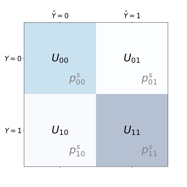
Figure 1: Confusion matrix in our setting - for each group $s$ we associate to $Y=i$ and $\hat{Y}=j$ the utility $U_{ij}$ and the probability $p^{s}_{ij}$. The true positives are represented by $p^{s}_{11}$, since $Y=1$ is considered the positive case.

Example 1 (University admission).

Admission to the university ($\hat{Y}=1$) offers a high utility if the study is completed. Failing to complete one’s studies often results in significant financial loss, encompassing both direct costs and the foregone opportunities of alternative paths. Therefore,

$$U_{11}\gg U_{01}$$ (1)

indicating that the utility derived from successfully completing studies (the case $11$) is substantially greater (indicated by $\gg$) than that from not completing them (the case $01$). For the case of no admission, we could neglect the utility difference, but it seems also plausible that in the case where $Y=1$ (indicating the capability to successfully complete the studies) the performance in other professional areas is higher in comparison to $Y=0$.

Fairness and inequality

It is common in the fairness literature to rely on a number of well-known statistical measures. We will refrain from a detailed discussion but only show a simple example here. A more detailed discussion is developed in (Fadina, Hinsch, and Schmidt 2024).

Disadvantages in terms of utilities

The central aim of our work is to measure inequalities by the means of utilities. In contrast to manifold other approaches we therefore do not rely on narrow statistical measures. Note that if the utility function is chosen to be the identity, we are considering monetary outcomes directly, and thus the detection of material inequality is contained as a special case. However, working with utilities allows a more general viewpoint, which we adopt here.

To ease the exposition we concentrate on two groups, i.e. $N=1$, while the arguments extend also to the general case. It is typically considered unfair if the algorithm produces unjustified disadvantages. Disadvantage will be measured in terms of utility difference between the groups. We do not aim at a distance, but a directed quantitiy. To this end, define $s=0$ as the standard group and $s=1$ as the protected group. We denote by $P_{s}$ the probability conditional on $s\in\{0,1\}$ and by $E_{s}$ the associated expectation.

A disadvantage (for the protected group) is a positive utility difference $\operatorname{UD}$ where

$$\operatorname{UD}:=E_{0}[U]-E_{1}[U].$$ (2)

If the utility difference is negative, the outcome for the protected group is better in comparison to the standard group, such that there is no disadvantage. Small disadvantages might be acceptable, and we fix a size $\tau\geq 0$ as a level of acceptable differences (in terms of utilities). A utility difference above $\tau$ is classified as a not negligible disadvantage of the protected group, which leads to the following definition.

Definition 2.

A decision rule induces a (not negligible) disadvantage, if

$$\operatorname{UD}>\tau.$$ (3)

In the following, by fairness we refer to the case where there is no disadvantage (at level $\tau=0$). Sometimes we also use the term fairness in utility to emphasize the difference to other fairness metrics.

Expected utility

Our first result computes the expected utility in our setting. It turns out that this expression can be simplified in the case with two groups only, while an analogous expression can obtained in a similar manner for arbitrarily many groups.

Proposition 3.

Assume that there are only two groups, i.e. $N=1$. Then, the expected utility for group $s$ is given by

$$E_{s}[U] =P_{s}(Y=1,\,\hat{Y}=1)\cdot(U_{11}-U_{01})$$

$$+P_{s}(Y=0,\,\hat{Y}=0)\cdot(U_{00}-U_{10})$$

$$+P_{s}(\hat{Y}=1)\cdot(U_{01}-U_{10})+U_{10}.$$ (4)

To provide an easy access to this formula we introduce the following notation:

$$\mathbf{U}:=\begin{pmatrix}U_{11}-U_{01}\\ U_{00}-U_{10}\\ U_{01}-U_{10}\end{pmatrix},\qquad\mathbf{P}_{s}:=\begin{pmatrix}P_{s}(Y=1,\hat{Y}=1)\\ P_{s}(Y=0,\hat{Y}=0)\\ P_{s}(\hat{Y}=1),\end{pmatrix}$$

such that

$$E_{s}[U]=\mathbf{U}\cdot\mathbf{P}_{s}+U_{10}.$$ (5)

The following proposition draws the connection to probabilities: if the joint probabilities of both groups coincide, then fairness holds. This also implies that all partial statistics (conditional use accuracy, positive predictive value, etc.) do not guarantee fairness without further assumptions.

Proposition 4 (Equal joint probabilities imply fairness).

Consider the case with two groups, i.e. $N=1$. If

$$P_{0}(\hat{Y}=i\,,\,Y=j)=P_{1}(\hat{Y}=i\,,\,Y=j),$$

for at least three pairs $(i,j)\in\{0,1\}\times\{0,1\}$, then the decision rule does not induce a disadvantage.

Since probabilities sum up to one, we do not need all four pairs $(i,j)$, and can reduce to three in the above results.

Computing the utility difference

We now introduce the appropriate tools to compute the utility difference $\operatorname{UD}$ easily in our setting with two groups, i.e. $N=1$. Then we have the associated probability measures $P_{0}$ and $P_{1}$ and introduce the difference

$$\operatorname{PD}(A):=P_{0}(A)-P_{1}(A)$$ (6)

for all sets $A$. From equation (5) we obtain that

$$\operatorname{UD}=\mathbf{U}\cdot\mathbf{PD}$$ (7)

where the vector $\mathbf{PD}=\mathbf{P}_{0}-\mathbf{P}_{1}$ can also be computed through the probability differences

$$\mathbf{PD}:=\begin{pmatrix}\operatorname{PD}(Y=1,\hat{Y}=1)\\ \operatorname{PD}(Y=0,\hat{Y}=0)\\ \operatorname{PD}(\hat{Y}=1)\end{pmatrix}.$$

The unfairness of $\varepsilon$-fairness

A general notion of fairness relies on a measure which describes the fairness of a certain decision rule $\hat{Y}$. From the above discussion we see that the question of fairness depends on the full joint distribution between groups. As a consequence, fairness can be related to a certain distance of these measures. Let us denote this distance by $d$. We say that the estimator $\hat{Y}$ achieves $d$-fairness if

$$d(P_{s_{1}},P_{s_{2}})=0.$$ (8)

In reality, it will typically not be possible to achieve a vanishing distance. In particular, since the probabilities need to be estimated, even if the distance vanishes on the estimated probabilities, this of course does not guarantee (maybe even not with a high probability) that the distance of the true underlying probability measures vanishes. Therefore it is natural to relax this notion in the following way: $\hat{Y}$ achieves $(d,\varepsilon)$-fairness if

$$d(P_{s_{1}},P_{s_{2}})\leq\varepsilon.$$ (9)

If the metric is clear from the context, we simply talk about $\varepsilon$-fairness.

The main goal of this section is to show that under certain assumptions $(d,0)$-fairness ensures utility-fairness, while this is not the case for $(d,\varepsilon)$-fairness. In fact, we provide an example which is $(d,\varepsilon)$- fair for an $\varepsilon>0$ arbitrary close to zero but is unfair in utility (even more, it is unfair on an arbitrarily large scale).

For all usual metrics $d$, a positive distance

$$d(P_{0},P_{1})>0$$ (10)

implies that at least one of the distances $|\operatorname{PD}(Y=0,\,\hat{Y}=0)|$, or $|\operatorname{PD}(Y=1,\,\hat{Y}=1)|$ is positive, hence

$$|\operatorname{PD}(Y=0,\,\hat{Y}=0)|+|\operatorname{PD}(Y=1,\,\hat{Y}=1)|>0.$$ (11)

The following results shows that $\varepsilon$-fairness can be maximally unfair. In particular, if the distance of the probability measures is not zero (but very small), the utility difference can be arbitrarily large.

Proposition 5.

Assume that $d(P_{0},P_{1})>0$ such that (11) holds. Then, there exist for any $K>0$ parameters $U_{00},\dots,U_{11}$ such that

$$\operatorname{UD}\geq K.$$

We may point to the simple proof of this proposition in the appendix which illustrates that for each possible scenario the utilities can be chosen in such an inconvenient way implying an arbitrarily large utility difference. In practice, however, there should be natural bounds on the utilities available. For this case we develop a number of tools in the following.

Without further assumptions we can at most hope for the following upper bound. Having Equation (7) in mind, we say that utility differences are bounded by $K$ if the vector $\mathbf{U}=(U_{1},U_{2},U_{3})^{\top}$ satisfies

$$\max\{|U_{1}|,|U_{2}|,|U_{3}|\}\leq K$$

and the probability differences are bounded by $\varepsilon$, if the vector $\mathbf{PD}=(\operatorname{PD}_{1},\operatorname{PD}_{2},\operatorname{PD}_{3})^{\top}$ satisfies

$$\max\{|\operatorname{PD}_{1}|,|\operatorname{PD}_{2}|,|\operatorname{PD}_{3}|\}\leq\varepsilon.$$

Proposition 6.

Assume that utility differences are bounded by $K>0$ and probability differences by $\varepsilon>0$. Then, there is no disadvantage larger than

$$3\hskip 0.86108pt\varepsilon K.$$

Demographic parity and equalized odds

There is an intensive discussion of which metrics should be used to study fairness of an algorithm. One metric which is of interest in the fairness discussion is demographic parity. In our context demographic parity arises naturally, compare Equation (7). Indeed, demographic parity holds if

$$P_{0}(\hat{Y}=1)=P_{1}(\hat{Y}=1),$$

and hence $\operatorname{PD}(\hat{Y}=1)=0.$ We say that statistical parity holds when

$$P_{0}(Y=1)=P_{1}(Y=1).$$

A further metric which is often discussed, is equalized odds. This measure requires equal true positive and false positive rates, i.e.

$$P_{0}(\hat{Y}=i|Y=i)=P_{1}(\hat{Y}=i|Y=i),i=0,1.$$ (12)

The following proposition shows that equalized odds together with statistical parity implies fairness. However, since statistical parity can not be controlled and will often not hold, this should rather rarely be applicable in practice.

Proposition 7.

Assume that statistical parity and equalized odds hold and that $U_{01}=U_{10}$. Then, there is no disadvantage.

We note that demographic parity together with equalized odds is not sufficient to conclude fairness.

College admission

As an example of our framework, we study college admission in further detail, extending Example 1. The study in (Webber 2016) shows that besides, age, education, race and gender also cognitive and non-cognitive abilities play an important role. For the first case we consider two groups which have median abilities but otherwise only differ in the protected attribute. For this case, the above study reports expected life-time earnings in the case with high college expenses of approximately 1,420,000 (high school) and 1,590,000 (some college). Thus, the utility of successfully completing the studies equals (in monetary terms)

$$U_{11}=170{,}000.$$

A first, rough estimate

Proposition 6 gives us a first rough estimate on possible disadvantages. With (14) we obtain $K=230.000$ as minimal bound on the utilities in this case. If a small $\varepsilon$ could be achieved this would already lead to a good bound. However, we will motivate in the following paragraph that the protected group typically has substantial disadvantages in completing their studies (say 20%) such that probability differences are bounded by $q_{0}\cdot 0.2=0.16$ in the later example. This implies

$$\operatorname{UD}\leq 0.16\cdot 230{,}000=36{,}800$$

which is substantial. Despite the fact that demographic parity holds in this case as we detail in the following.

The simplest case

Additionally, we assume $U_{01}=0$, since we see this as our reference case here. Also let us assume for this case that $U_{10}=U_{00}=0$. It is clear that university admission is highly attractive and everybody should have equal opportunities to participate.

We again assume that group $0$ is admitted with probability $q_{0}\in[0,1]$ and the protected group $1$ with probability $q_{1}\in[0,1]$. The algorithm has some forecasting abilities, and hence $Y$ is not independent from $\hat{Y}$. However failure rates are still reported to be high and we assume that the forecast is little worse in the protected group, possibly due to lack of data or other factors. We introduce $\delta>0$ as follows:

$$P_{0}(Y=1\,|\,\hat{Y}=1) =P_{1}(Y=1\,|\,\hat{Y}=1)+\delta$$

$$>P_{1}(Y=1\,|\,\hat{Y}=1)=:q_{1}(1,1);$$

where we denote $q_{s}(i,j)=P_{s}(Y=i\,|\,\hat{Y}=j)$. Then,

$$\operatorname{UD} =\mathbf{U}\cdot\mathbf{PD}$$

$$=\begin{pmatrix}U_{11}\\ 0\\ 0\end{pmatrix}\cdot\begin{pmatrix}q_{0}\cdot(q_{1}(1,1)+\delta)-q_{1}\cdot q_{1}(1,1)\\ (1-q_{0})\cdot q_{0}(0,0)-(1-q_{1})\cdot q_{1}(0,0)\\ q_{0}-q_{1}\end{pmatrix}$$

$$=U_{11}\cdot\big{(}q_{1}(1,1)\cdot(q_{0}-q_{1})+q_{0}\cdot\delta\big{)}.$$ (13)

The simplicity of this formula stems from our assumptions, since only $U_{11}$ was assumed to be non-vanishing, while all other utilities vanish.

At this moment two things become clear: demographic parity (i.e. $q_{0}=q_{1}$) only implies no disadvantages if $\delta=0$. In this case,

$$\operatorname{UD}_{q_{0}=q_{1}}=U_{11}\cdot q_{0}\cdot\delta=0.$$

If the standard group is admitted with, say $q_{0}=80\%$, and the prediction difference $\delta$ is substantial, say $\delta=20\%$, then the utility difference computes to 27,200.

We compute the smallest level of admission probabilities for the protected group which implies no disadvantages. We assume that $q_{1}(1,1)=70\%$, i.e. 30% failure rate. Then,

$$q_{1}^{*}=\frac{q_{1}(1,1)\cdot q_{0}+q_{0}\cdot\delta}{q_{1}(1,1)}=q_{0}\cdot\Big{(}1+\frac{\delta}{q_{1}(1,1)}\Big{)}>1.00.$$

Summarizing, from our viewpoint an admission rate of over 100% is the minimal admission rate to ensure no disadvantage. The advantage of university admission in this case is so high that almost everyone from the protected group should be admitted to correct for the disadvantage arising through the more insecure prediction through $\delta$. With an admission rate of 100% still a disadvantage of 500 remains. It turns out that more needs to be done to achieve fairness: the failure rates of the protected group need to be reduced, a surprisingly strong result from our simple framework.

We illustrate the situation in Figure 2. On the left hand side we modify the setup slightly, by considering a fixed number of possible admissions, which improves the situation a bit (we do not detail the simple calculations).

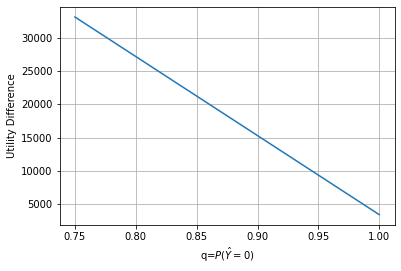
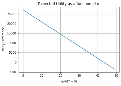
Figure 2: Utility differences for the college admission. Left:The utility difference as function of $q_{1}$. Even if the admission rate of the protected group equals $q_{1}=100\%$, there remains a disadvantage of ca. 500. Right: The case with a fixed number of admitted persons. We admit 1000 persons out of 1250, where 250 belong to the protected group. Starting from an equal admission rate of 80% we allow additional persons from the protected group, meanwhile diminishing the number of admissions from the other group. In this case one is able to achieve equal utilities by admitting 95% of the protected group.

Incorporating student loans

Now we may revisit that case, incorporating remaining student loans when studies are not completed successfully. According to (Webber 2016) high college costs were on average leading to a loan of size 60,000, i.e.

$$U_{01}=-60{,}000.$$ (14)

In this case, we obtain

$$\operatorname{UD}=\mathbf{U}\cdot\mathbf{PD}$$

$$=\begin{pmatrix}U_{11}-U_{01}\\ 0\\ U_{01}\end{pmatrix}\cdot\begin{pmatrix}q_{0}\cdot(q_{1}(1,1)+\delta)-q_{1}\cdot q_{1}(1,1)\\ (1-q_{0})\cdot q_{0}(0,0)-(1-q_{1})\cdot q_{1}(0,0)\\ q_{0}-q_{1}\end{pmatrix}$$

$$=(U_{11}-U_{01})\cdot\big{(}q_{1}(1,1)\cdot(q_{0}-q_{1})+q_{0}\cdot\delta\big{)}$$

$$+U_{01}\cdot(q_{0}-q_{1}).$$ (15)

We first observe that now $U_{11}$ is replaced by

$$U_{11}-U_{01}=230{,}000,$$

such that the previously discussed effect is increased by more than one fourth. Demographic parity ($q_{0}=q_{1}$) in this case eliminates the second component of the utility difference (see Equation (15)).

Taking wealth into account

Up to now we presented fairly general results and concentrated on monetary inequality. However, the utility-based framework offers much more, for example different wealth between the groups or even on an individual level can be taken into account through a utility function. In this case, the utilities will depend on the group. This can be incorporated into our framework, but is beyond the scope of this paper and therefore left for future research.

Sufficient conditions

The preceding results showed that one has to be extremely careful when considering fairness, in particular when the context is left aside. In the following we will show how to come up with useful estimates which allow to conclude a suitable level of fairness even when the utilities are not known precisely. In the case when some utilities vanish, we may reduce our requirements even further and can conclude fairness on the basis of some well-known requirements.

Conditional use accuracy

While many conditional quantities like true positive rate or equalized odds typically do not imply equality of the unconditional probabilities they are difficult to connect to Equation (5).

This is simpler with the conditional use accuracy, which we will exploit now. In principle this can also be applied to equalized odds, but not without a few additional steps, such that we do not consider this quantity here.

According to (Caton and Haas 2024) Section 3.2.2, equality in the conditional use accuracy (CUA) holds, if

$$\operatorname{PD}(Y=i\,|\,\hat{Y}=i)=0$$

for $i=0,1$.

Recall that by no disadvantage in the sense of Definition 2 we mean a vanishing (or negative) utility difference, i.e. $\operatorname{UD}\leq 0$. For the following proposition we denote by $\Gamma\in[0,1]$ the number

$$\Gamma=\max\{P_{0}(Y=1\,|\,\hat{Y}=1);P_{0}(Y=0\,|\,\hat{Y}=0)\}.$$ (16)

Note that under CUA, $P_{0}$ can be replaced by $P_{1}$ for the computation of $\Gamma$.

Proposition 8.

Assume that equality of the conditional use accuracy holds.

1. If $P_{0}(\hat{Y}=1)=P_{1}(\hat{Y}=1)$, then there is no disadvantage.

2. If the utility differences are bounded by $K>0$ and $|P_{0}(\hat{Y}=1)=P_{1}(\hat{Y}=1)|\leq\varepsilon$, then there is no disadvantage larger than

   $$(1+2\Gamma)\cdot\varepsilon\cdot K.$$

In comparison to Proposition (6), CUA allows to reduce the general bound further, in particular if $\Gamma$ is small. The second result shows that if $(1+2\Gamma)\varepsilon K\leq\tau$ for the level $\tau$ in Definition 2, there are only negligible disadvantages. In our examples $K$ turns out to be quite small, such that this seems to be a result highly relevant for practical cases.

Independence

An abstract criterion for fairness (on the probability level only) which immediately makes sense is independence, see (Caton and Haas 2024) Section 3.1, for example. We will show that independence also implies absence of disadvantages and, hence, fairness in the sense we consider here - but is not necessary. In essence, it is to strict. It also turns out that independence of the estimator $\hat{Y}$ and the group alone is not sufficient.

To consider independence, assume that the group $S$ is a random variable. Our probability measures $P_{s}$ are then obtained by conditioning on $S=s$.

Proposition 9.

Independence of $(Y,\hat{Y})$ and $S$ implies absence of a disadvantage.

The reduced setting

In many situations there is not enough information about the probability of the cases $\{Y=0,\hat{Y}=0\}$ and $\{Y=1,\hat{Y}=0\}$: in the college admission this would refer to the probability of successfully completing the studies while not being admitted to the university, a probability which is clearly difficult to estimate.

To additionally capture these important situations within our framework, we introduce the reduced setting: here, both cases (00 and 01) are collapsed into the case 0 (referring to $\hat{Y}=0$) and hence only the probability

$$p^{s}_{0}:=P_{s}(\hat{Y}=0)$$

is needed, see Figure 3 for an illustration.

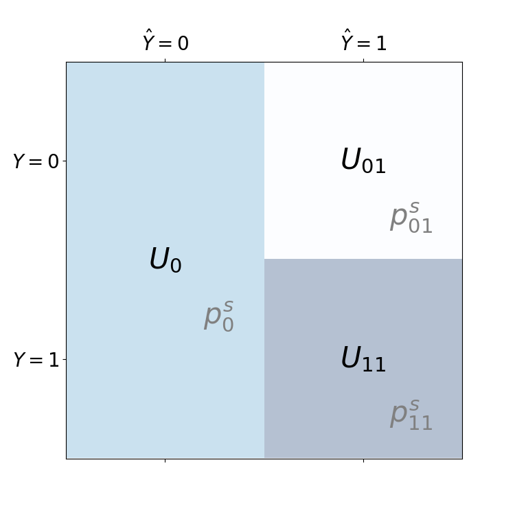
Figure 3: Confusion matrix in the reduced setting. The cases 00 and 10 are now collapsed to the case $0$ (where $\hat{Y}=0$).

Note that the results for the reduced setting can be obtained as a special case of the standard case by letting $U_{10}=U_{00}=U_{0}$.

Lemma 10.

The expected utility in the reduced setting is

$$E_{s}[\tilde{U}]=\tilde{\mathbf{U}}\cdot\tilde{\mathbf{P}}_{s}+U_{0}.$$ (17)

with

$$\tilde{\mathbf{U}}:=\begin{pmatrix}U_{11}-U_{01}\\ U_{01}-U_{0}\end{pmatrix},\qquad\tilde{\mathbf{P}}_{s}:=\begin{pmatrix}P_{s}(Y=1,\hat{Y}=1)\\ P_{s}(\hat{Y}=1).\end{pmatrix}$$

In the college example we were already working in a reduced setting since we assumed $U_{00}=U_{10}=0$.

Sufficient conditions in the reduced setting

We adopt the conditional use accuracy to this setting. Since $\{Y=0|\hat{Y}=0\}$ is not available, we replace this by the unconditional $\hat{Y}=0$ and call it the (conditional) use accuracy, (C)UA. It holds if

$$\begin{aligned} \operatorname{PD}(Y=1\,|\,\hat{Y}=1)&=0,\\ \operatorname{PD}(\hat{Y}=0)&=0.\end{aligned}$$ (18)

We immediately obtain the following result from Proposition 8

Proposition 11.

Assume that equality of the (conditional) use accuracy holds, i.e. (18). Then there is no disadvantage.

A mortgage example

As an example where it is important to consider the context for an in-depth analysis of fairness, we consider credit ratings used in the context of mortgages. It also illustrates the importance of the reduced setting - since there is no data on people who were rejected on a mortgage application. In contrast to smaller credits, the mortgage case is much more involved. We take some time to show how a fundamental model can be developed and what are the conclusions drawn. We start with a simplified setting and then illustrate the full power of the utility-based approach.

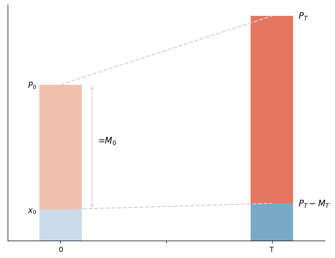
Figure 4: Illustration of the mortgage example

For the mortgage, we look at the evolution over time, starting at time $t=0$ and ending with the payback time $T>0$. Consider a mortgage of size $M_{0}$ for a house of price $P_{0}$ and assume that the individual has liquid capital $x_{0}$. For simplicity, we assume $M_{0}=P_{0}-x_{0}$. The value of the house changes over time and its value at time $T$ is denoted by $P_{T}$. The creditor saved the amount $x_{T}$ until time $T$.

First, if $X_{T}\geq M_{T}$ there is no default. Second, if $X_{T}<M_{T}$, there is default and the house has to be sold. This typically can only be sold at a lower price, which we denote by $P_{T}\cdot(1-\lambda)$ with $\lambda\geq 0$.

Now, if $P_{T}\cdot(1-\lambda)+X_{T}\geq M_{T}$, the bank has no loss - the full mortgage can be covered. However, the creditor ends up with a possibly small fraction

$$P_{T}\cdot(1-\lambda)+X_{T}-M_{T}.$$

If $P_{T}\cdot(1-\lambda)+X_{T}<M_{T}$, the bank receives what is left,

$$\big{(}P_{T}\cdot(1-\lambda)+X_{T}\big{)}^{+},$$

and faces a (typically small) financial loss.

This already gives the impression that the risk for the bank is quite small, but the risk for the creditor is substantial. In particular in the case of default, the situation for the creditor is difficult and associated with a highly negative utility.

Reduced setting

We first simplify the setting and view the approach from a purely data-based point of view, as it is often done in this case. In this case we end up in the reduced setting introduced above.

We note that in the reduced setting we have to specify utilities for the cases $U_{11},\ U_{01}$ and the case $U_{0}$ together with associated probabilities. We think of a house costing $P_{0}=300{,}000$ and the creditor has capital of 30%, such that the needed mortgage equals $M_{0}=210{,}000$. Assume that with a probability of $95\%$ no default happens. The associated utility is

$$U_{11}=400{,}000-90{,}000=310{,}000$$

through the rise in the value of the house minus the initial capital. On the other side, in case of default the house can be sold at 300,000 in the good case and 200,000 in the bad case and we consider the average. Hence,

$$U_{01}=250{,}000-90{,}000=160{,}000.$$

In the case of no mortgage, the living cost $C=100{,}000$ is computed by using $T=10$ and approx. 3% of the house value as yearly rent. Thus,

$$U_{0}=200{,}000+90{,}000-100{,}000=190{,}000,$$

where we assumed that only little less than $M_{0}$ is earned on average over the 10 years. In contrast to the college admission, $U_{0}$ does not vanish and is even larger than $U_{10}$. It is therefore better not to get the mortgage when the likelihood of default is substantial.

We consider an equal acceptance rate between both groups, $P_{0}(\hat{Y}=1)=P_{1}(\hat{Y}=1)=0.8$. Conditionally on acceptance we assume that 95% of the standard group does not default while 90% of the protected group does not default. In this case the setting will clearly be unfair - and our question will be how to remedy this. First we compute the utility difference according to Equation (17),

$$\tilde{\operatorname{UD}} =\begin{pmatrix}150{,}000\\ -30{,}000\end{pmatrix}\cdot\begin{pmatrix}0.76-0.72\\ 0.8-0.8\end{pmatrix}=6{,}000.$$

First, we observe that $\tilde{U}_{2}$ is negative (in contrast to being zero as in the college admission). Second, the small change in the default probability results in a difference which is 4% of 150.000. Since default probabilities can not be changed in this situation (although this is of course an important aspect of fairness) we aim at changing the acceptance rate for the protected group to obtain a situation where both groups have equal utilities.

Quite surprising, decreasing the acceptance rate improves the utility for the protected group: we need to solve

$$-30{,}000\cdot(0.8-p)=-60{,}000,$$

and we find $p=0.6$. Thus, with a reduced acceptance rate for the protected group of 0.6 the setting turns out to be fair in the sense that there is no disadvantage for the protected group. The reason for this is that in the case of default the situation is disadvantageous. Thus, simply aiming at equal acceptance rates actually turns out to lead to a disadvantage in utility for the protected group - clearly an unwanted effect.

Accounting for uncertainty

Up to now we assumed that the probability measures where given and exactly known. This is of course not true in practice where probabilities have to be estimated. While the estimator carries significant uncertainty, this can be reduced by considering confidence intervals. In this section, we extend our previous setting by working on uncertainty sets, which could be obtained from confidence intervals or, in the spirit of Knightian uncertainty, by a combination with expert opinions or other data sources.

To simplify the approach we remain in the reduced setting from Equation (17), while the standard setting can be treated in the same manner.

To this end we denote the estimated probabilities by $\pi$ - the uncertainty interval will be represented by $[\underline{\pi},\overline{\mathrlap{\pi}\phantom{\underline{\pi}}}].$ In this spirit, the uncertainty interval for $\tilde{\mathbf{P}}_{s}$ is denoted by the two intervals

$$\begin{matrix}[\underline{\pi}_{s}(Y=1,\hat{Y}=1)\,,\,\overline{\mathrlap{\pi}\phantom{\underline{\pi}}}_{s}(Y=1,\hat{Y}=1)]\\[5.69054pt] [\underline{\pi}_{s}(\hat{Y}=1)\,,\,\overline{\mathrlap{\pi}\phantom{\underline{\pi}}}_{s}(\hat{Y}=1)]\end{matrix}$$ (19)

Proposition 12.

Assume that $\tilde{\mathbf{U}}\geq 0$. Then, the upper bound of the utility difference is given by

$$\overline{\operatorname{UD}}=\tilde{\mathbf{U}}\cdot\Pi^{*}$$ (20)

with

$$\Pi^{*}=\begin{pmatrix}\overline{\mathrlap{\pi}\phantom{\underline{\pi}}}_{0}(Y=1,\hat{Y}=1)-\underline{\pi}_{1}(Y=1,\hat{Y}=1)\\ \overline{\mathrlap{\pi}\phantom{\underline{\pi}}}_{0}(\hat{Y}=1)-\underline{\pi}_{1}(\hat{Y}=1)\end{pmatrix}.$$ (21)

Confidence intervals

Depending on the chosen approach, estimating confidence intervals could be challenging. While for logistic regression, a common statistical approach to categorial classification, this is well-known, it might be less known that also for ML-algorithms like random forests, there are known approaches to estimate confidence intervals. For example, one may rely on the jackknife estimator, see (Wager, Hastie, and Efron 2014).

Beyond this we would like to remark that some subtleties should be taken into account: first, recall that we considered no covariables (up to now), i.e. the individuals which we consider should have the same or at least similar levels of the covariables. This could be the same credit rating, the same post code, a similar gpa, etc. Moreover, the data should be i.i.d. - which might not be the case if many years are considered, which also needs to be taken into account. Since smaller sample sizes increase the confidence intervals, we expect that this is important for many cases.

Outlook on a general setting

In the general setting we introduce a probabilistic model of the default along the line of the famous Merton model, (Merton 1974), with an adaptation to the mortgage case. A more detailed modelling would require treating imperfect information as in (Stiglitz and Weiss 1981; Frey and Schmidt 2009) and will be treated in future work. The following steps also serve as a guideline on how explicit biases in existing data could be modelled or how the approach could be applied in more complex questions which can not be treated by the standard setting in Equation (5).

Let us assume that the future wealth $X_{T}$ is normally distributed with mean $\mu$ and standard deviation $\sigma$. Denote the difference in income by $\Delta X_{T}=X_{T}-x_{0}$. At time $T$ we have that the utility of the creditor is given by

$$U=\begin{cases}P_{T}+\Delta X_{T}-M_{T}&X_{T}>M_{T},\\ P_{T}\cdot(1-\lambda)+\Delta X_{T}-M_{T}&D_{1},\\ -x_{0}&D_{2},\end{cases}$$

where $D_{1}$ denotes the default case where $P_{T}\cdot(1-\lambda)+X_{T}>M_{T}$ and $D_{2}$ denotes the default case where $P_{T}\cdot(1-\lambda)+X_{T}\leq M_{T}$.

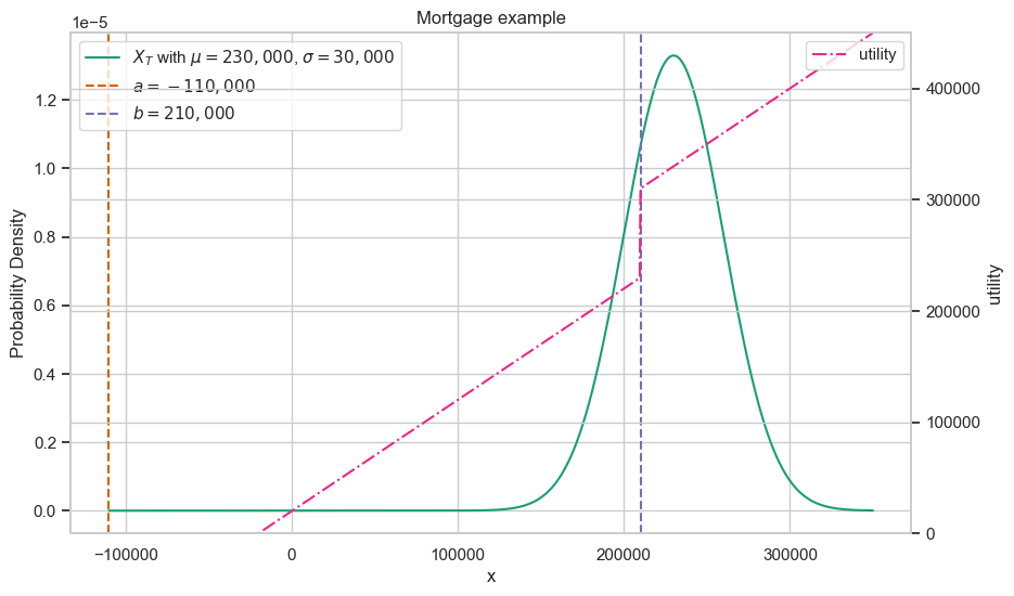
Figure 5: Illustration of the general setting - the income $X_{T}$ is normally distributed and we plot the density, together with the two utility barriers - $D_{1}$ is between $a$ and $b$ - and the utility $U$.

As a first result we compute the distribution of $U$ together with its expected utility. Note that the case $11$ corresponds to no default, while $01$ corresponds to the default case (which in our case contains $D_{1}$ and $D_{2}$). Thus $P(Y=1,\hat{Y}=1)=P(X_{T}>M_{T})$ while $P(Y=0,\hat{Y}=1)=1-P(X_{T}>M_{T})=P(D_{1})+P(D_{2})$. Utilities in the case where the mortgage is not admitted is easily computed and equals $U_{0}=x_{0}+E[X_{T}]=x_{0}+\mu-C$ where $C$ includes additional costs due to lending. By $D=D_{1}+D_{2}$ we denote the event that default occurs, such that the probability of default equals $P(D)$.

Lemma 13.

Under the above assumptions, we have

$$P(X_{T}>M_{T})=\Phi\Big{(}\frac{\mu-M_{T}}{\sigma}\Big{)}=1-P(D),$$

$$P(D_{1})=\Phi\Big{(}\frac{M_{T}-\mu}{\sigma}\Big{)}-\Phi\Big{(}\frac{M_{T}-P_{T}\cdot(1-\lambda)-\mu}{\sigma}\Big{)},$$

$$P(D_{2})=\Phi\Big{(}\frac{M_{T}-P_{T}\cdot(1-\lambda)-\mu}{\sigma}\Big{)},$$

$$E[U_{11}|=\big{(}P_{T}+\mu-x_{0}-M_{T})\cdot\Phi\big{(}\frac{\mu-M_{T}}{\sigma}\Big{)}$$

$$\phantom{E[U_{11}]}+\sigma\phi\Big{(}\frac{\mu-M_{T}}{\sigma}\Big{)},$$

$$E[U_{01}]=-x_{0}\cdot P(D)+\big{(}P_{T}(1-\lambda)+\mu-M_{T}\big{)}\cdot P(D_{1})$$

$$\phantom{E[U_{01}]}+\sigma\Big{(}\phi\Big{(}\frac{M_{T}-P_{T}(1-\lambda)-\mu}{\sigma}\Big{)}-\phi\Big{(}\frac{M_{T}-\mu}{\sigma}\Big{)}\Big{)},$$

$$E[U_{0}]=x_{0}+E[X_{T}]=x_{0}+\mu-C.$$

For an illustration, we compute the related values in correspondence to our previous mortgage example. We then have $M_{T}=M_{0}=200{,}000$, $P_{T}=400{,}000$, $x_{0}=90{,}000$ and $C=100{,}000$. For illustration we expect that the average income is higher than the mortgage, such that $\mu=M_{T}+20{,}000$ (not too high to see a significant default probability) and $\sigma=30{,}000$ together with a $\lambda=0.2$, see Figure 5. The default probability then computes to 25% and $E[U_{11}]=256{,}000$, $E[U_{01}]=54{,}000$ and $E[U_{0}]=220{,}000$ showing a similar relation between the utilities as in the previous example.

Changing the mean to $\mu=M_{T}+50{,}000$ allows to adjust the default probability, which then computes to 5% together with $E[U_{11}]=345{,}000$, $E[U_{01}]=10{,}000$ and $E[U_{0}]=250{,}000$, even more showing that the utility in the default case is far away from the utility in the non-default case or from the case where the credit is not offered. Computation of utility differences under several model assumptions is now straightforward. A detailed discussion, however, is beyond the scope of this short paper.

Summarizing, this small illustration of a general utility-based approach confirms the findings in our reduced-setting: fairness measured only on statistical measures is out of context and may be highly unfair if measured in utilities. To mitigate unfairness in the mortgage example not only acceptance rates have to be adjusted but also precautionary measures have to be taken into account to lower the highly unwanted effects when default occurs.

Conclusion

This paper introduces a simple and tractable framework for measuring fairness in terms of utilities. We show that previously considered measures do not necessarily guarantee fair outcomes from this more holistic viewpoint, in particular the concept of $\varepsilon$-fairness might lead to wrong assessments. We also provide illustrating examples and mathematical tools which may serve as a useful basis for further applications.

Appendix A Proofs

Proposition 3.

Assume that there are only two groups, i.e. $N=1$. Then, the expected utility is given by

$$E[U] =P(Y=1,\,\hat{Y}=1)\cdot(U_{11}-U_{01})$$

$$+P(Y=0,\,\hat{Y}=0)\cdot(U_{00}-U_{10})$$

$$+P(\hat{Y}=1)\cdot(U_{01}-U_{10})+U_{10}.$$

Proof.

The overall utility is given by summing over all possible states, i.e.

$$U=\sum_{k,j=0}^{1}{\mathds{1}}_{\{Y=k,\hat{Y}=j\}}U_{kj}.$$

Hence, the expected utility equals

$$E[U] =\sum_{k,j=0}^{1}P(Y=k,\hat{Y}=j)\cdot U_{kj}.$$ (22)

Now let us concentrate on $j=1$. We obtain that

$$P(Y=0\,,\,\hat{Y}=1)=P(\hat{Y}=1)-P(Y=1\,,\,\hat{Y}=1).$$

Hence, inserting this into Equation (22),

$$E[U{\mathds{1}}_{\{\hat{Y}=1\}}] =P(\hat{Y}=1)\cdot U_{01}$$

$$+P(Y=1\,,\,\hat{Y}=1)\cdot(U_{11}-U_{01}).$$ (23)

Similarly, $P(Y=1\,,\,\hat{Y}=0)=P(\hat{Y}=0)-P(Y=0\,,\,\hat{Y}=0)$, such that

$$E[U{\mathds{1}}_{\{\hat{Y}=0\}}] =P(\hat{Y}=0)\cdot U_{10}$$

$$+P(Y=0\,,\,\hat{Y}=0)\cdot(U_{00}-U_{10})$$ (24)

and the conclusion follows by summing (A) and (A) and using that $P(\hat{Y}=0)=1-P(\hat{Y}=1)$. ∎

Proposition 5.

Assume that $d(P_{0},P_{1})>0$ such that (11) holds. Then, there exist for any $K\geq 0$ parameters $U_{00},\dots,U_{11}$ such that

$$\operatorname{UD}\geq K.$$

Proof.

The core of the argument is representation (7), which we repeat for convenience,

$$\operatorname{UD}=\begin{pmatrix}U_{11}-U_{01}\\ U_{00}-U_{10}\\ U_{01}-U_{10}\end{pmatrix}\cdot\begin{pmatrix}\operatorname{PD}(Y=1,\hat{Y}=1)\\ \operatorname{PD}(Y=0,\hat{Y}=0)\\ \operatorname{PD}(\hat{Y}=1).\end{pmatrix}$$

We set $U_{01}=U_{10}$, such that $\operatorname{UD}_{3}=0$. Equation (11) implies a number of cases which we can treat similarly. Consider for example $\operatorname{PD}(Y=1,\,\hat{Y}=1)>0$. We choose $U_{00}=U_{10}$ to obtain $\operatorname{UD}_{2}=0$. Then, we choose $U_{10}=0$ and $U_{11}=K\cdot\operatorname{PD}(Y=1,\,\hat{Y}=1)^{-1}>0$, such that

$$\operatorname{UD}=(U_{11}-U_{01})\cdot\operatorname{PD}(Y=1,\,\hat{Y}=1)=K.$$ (25)

The other results follow in a similar way. ∎

Proposition 7.

Assume statistical parity and equalized odds hold and that $U_{01}=U_{10}$. Then, there is no disadvantage.

Proof.

We begin by noting that Bayes’ formula implies that

$$P_{s}(Y=i)\cdot P_{s}(\hat{Y}=i|Y=i)=P_{s}(\hat{Y}=i,Y=i).$$

Thus, statistical parity together with equalized odds imply equal joint distributions on the diagonal. Since $U_{01}=U_{10}$, we obtain that $U_{3}=0$ and the claim follows from Equation (7). ∎

Proposition 8.

Assume that equality of the conditional use accuracy holds.

1. If $P_{0}(\hat{Y}=1)=P_{1}(\hat{Y}=1)$, then there is no disadvantage.

2. If the utility differences are bounded by $K>0$ and $|P_{0}(\hat{Y}=1)=P_{1}(\hat{Y}=1)|\leq\varepsilon$, then there is no disadvantage larger than

   $$(1+2\Gamma)\cdot\varepsilon\cdot K.$$

Proof.

For the first claim, observe that

$$\operatorname{PD}(Y=1,\hat{Y}=1) =P_{0}(Y=1,\hat{Y}=1)-P_{1}(\hat{Y}=1).$$

Note that by Bayes’ theorem,

$$P_{s}(Y=1,\hat{Y}=1)=P_{s}(\hat{Y}=1)\cdot P_{s}(Y=1|\hat{Y}=1)$$

for $s=0,1$. Since CUA implies that the conditional probabilities $P_{s}(Y=1|\hat{Y}=1)$, $s=0,1$ are equal it remains to consider the probabilities $P_{s}(\hat{Y}=1).$ This is exactly our assumption in (i) and it follows that the probability difference vanishes, i.e.

$$\operatorname{PD}(Y=1,\hat{Y}=1)=0.$$

For the probability difference $\operatorname{PD}(Y=0,\hat{Y}=0)$ observe that the assumption in (i) also implies $P_{0}(\hat{Y}=0)=P_{1}(\hat{Y}=0)$ and we obtain in a similar manner

$$\operatorname{PD}(Y=0,\hat{Y}=0)=0.$$

Since we also have $\operatorname{PD}(\hat{Y}=1)=0$, Proposition 4 implies absence of any disadvantage.

For the second claim we estimate the utility difference using Equation (4) by

$$|\operatorname{UD}|\leq K\cdot\parallel\operatorname{PD}\parallel_{\infty}$$

where $\parallel\operatorname{PD}\parallel_{\infty}$ denotes the maximum of the absolute values of the rows of the vector $\operatorname{PD}$. We examine the rows of $\operatorname{PD}$ separately. For the first row we argue as above, using Bayes’ theorem, and obtain that (again using CUA)

$$|\operatorname{PD}(Y=1,\hat{Y}=1)| \leq P_{0}(Y=1|\hat{Y}=1)\cdot|\operatorname{PD}(\hat{Y}=1)|$$

$$\leq P_{0}(Y=1|\hat{Y}=1)\cdot\varepsilon\leq\Gamma\cdot\varepsilon.$$

In an analogous manner we obtain a similar estimate for the second row and $\varepsilon\cdot K$ as a bound for the third row and the proof is finished. ∎

Proposition 9.

Independence of $(Y,\hat{Y})$ and $S$ implies absence of a disadvantage.

Proof.

Note that independence implies for all $i,j$ that

$$P_{0}(Y=i\,,\,\hat{Y}=j) =P(Y=i\,,\,\hat{Y}=j\,|\,S=0)$$

$$=P(Y=i\,,\,\hat{Y}=j)$$

$$=P_{1}(Y=i\,,\,\hat{Y}=j).$$

Now, Proposition 4 yields the result. ∎

Lemma 10.

The expected utility in the reduced setting computes to

$$E[\tilde{U}]=\tilde{\mathbf{U}}\cdot\tilde{\mathbf{P}}+U_{0}.$$

with

$$\tilde{\mathbf{U}}:=\begin{pmatrix}U_{11}-U_{01}\\ U_{01}-U_{0}\end{pmatrix},\qquad\tilde{\mathbf{P}}:=\begin{pmatrix}P(Y=1,\hat{Y}=1)\\ P(\hat{Y}=1).\end{pmatrix}$$

Proof.

As in Proposition 3,

$$E[U] =U_{11}\cdot P(Y=1,\hat{Y}=1)+U_{01}\cdot P(Y=0,\hat{Y}=1)$$

$$+U_{0}P(\hat{Y}=0).$$

Since $P(\hat{Y}=0)=1-P(\hat{Y}=1)$ and

$$P(Y=0,\hat{Y}=1)+P(Y=1,\hat{Y}=1)=P(\hat{Y}=1),$$

we obtain that

$$E[U] =(U_{11}-U_{01})\cdot P(Y=1,\hat{Y}=1)$$

$$+(U_{01}-U_{0})\cdot P(\hat{Y}=1)+U_{0}.$$

Putting this into the representation of the lemma, the result is proven. ∎

Lemma 11.

Under the above assumptions, we have

$$P(X_{T}>M_{T})=\Phi\Big{(}\frac{\mu-M_{T}}{\sigma}\Big{)}=1-P(D),$$

$$P(D_{1})=\Phi\Big{(}\frac{M_{T}-\mu}{\sigma}\Big{)}-\Phi\Big{(}\frac{M_{T}-P_{T}\cdot(1-\lambda)-\mu}{\sigma}\Big{)},$$

$$P(D_{2})=\Phi\Big{(}\frac{M_{T}-P_{T}\cdot(1-\lambda)-\mu}{\sigma}\Big{)},$$

$$E[U_{11}|=\big{(}P_{T}+\mu-x_{0}-M_{T})\cdot\Phi\big{(}\frac{\mu-M_{T}}{\sigma}\Big{)}$$

$$\phantom{E[U_{11}]}+\sigma\phi\Big{(}\frac{\mu-M_{T}}{\sigma}\Big{)},$$

$$E[U_{01}]=-x_{0}\cdot P(D)+\big{(}P_{T}(1-\lambda)+\mu-M_{T}\big{)}\cdot P(D_{1})$$

$$\phantom{E[U_{01}]}+\sigma\Big{(}\phi\Big{(}\frac{M_{T}-P_{T}(1-\lambda)-\mu}{\sigma}\Big{)}-\phi\Big{(}\frac{M_{T}-\mu}{\sigma}\Big{)}\Big{)},$$

$$E[U_{0}]=x_{0}+E[X_{T}]=x_{0}+\mu-C.$$

Proof.

Since $X_{T}$ is normally distributed, $X_{T}=M_{T}+\sigma\xi$ with mean $M_{T}$ and standard deviation $\sigma$. This already gives the first result. Next, $P(D_{1})=P(M_{T}-P_{T}(1-\lambda)<X_{T}\leq M_{T})$ which implies the second and the third equation.

The utility in the case $Y=1,\hat{Y}=1$ is given by

$$E[U_{11}] =E\Big{[}\big{(}P_{T}+X_{T}-x_{0}-M_{T}\big{)}{\mathds{1}}_{\{X_{T}>M\}}\Big{]}$$

$$=\big{(}P_{T}+\mu-x_{0}-M_{T}\big{)}\cdot P(X_{T}>M)$$

$$+\sigma\cdot E\Big{[}\xi\,{\mathds{1}}_{\{\xi>\frac{M_{T}-\mu}{\sigma}\}}\Big{]}.$$

Noting that

$$\int_{C}^{\infty}x\frac{1}{\sqrt{2\pi}}e^{-\frac{x^{2}}{2}}=\frac{1}{\sqrt{2\pi}}e^{-\frac{C^{2}}{2}}=\phi(C),$$

the fourth equation follows. In a similar way,

$$E[U_{01}] =E\Big{[}\big{(}P_{T}(1-\lambda)+X_{T}-x_{0}-M_{T}\big{)}\cdot$$

$$\qquad\qquad\cdot{\mathds{1}}_{\{M_{T}-P_{T}(1-\lambda)<X_{T}\leq M_{T}\}}\Big{]}$$

$$+E\Big{[}-x_{0}\cdot{\mathds{1}}_{\{X_{T}\leq M_{T}-P_{T}(1-\lambda)\}}\Big{]}$$

$$=-x_{0}\cdot P(D_{1}+D_{2})$$

$$+\big{(}P_{T}(1-\lambda)+\mu-M_{T}\big{)}\cdot P(D_{1})$$

$$+\sigma\cdot E\Big{[}\xi\,{\mathds{1}}_{\{M_{T}-P_{T}(1-\lambda)<X_{T}\leq M_{T}\}}\Big{]}.$$

Noting that

$$\int_{C_{1}}^{C_{2}}x\frac{1}{\sqrt{2\pi}}e^{-\frac{x^{2}}{2}}=\phi(C_{1})-\phi(C_{2}),$$

the fith equation follows. Since the last equation is immediate, the proof is finished. ∎

References

- Arrow (1973) Arrow, K. J. 1973. Some ordinalist-utilitarian notes on Rawls’s theory of justice.
- Ben-Porat, Sandomirskiy, and Tennenholtz (2021) Ben-Porat, O.; Sandomirskiy, F.; and Tennenholtz, M. 2021. Protecting the Protected Group: Circumventing Harmful Fairness. In Proceedings of the AAAI Conference on Artificial Intelligence, 35.
- Blandin and Kash (2023) Blandin, J.; and Kash, I. A. 2023. Generalizing Group Fairness in Machine Learning via Utilities. Journal of Artificial Intelligence Research, 78: 747–780.
- Caton and Haas (2024) Caton, S.; and Haas, C. 2024. Fairness in machine learning: A survey. ACM Computing Surveys, 56(7): 1–38.
- Dwork et al. (2012) Dwork, C.; Hardt, M.; Pitassi, T.; Reingold, O.; and Zemel, R. 2012. Fairness through awareness. In Proceedings of the 3rd innovations in theoretical computer science conference, 214–226.
- Dwork, Reingold, and Rothblum (2023) Dwork, C.; Reingold, O.; and Rothblum, G. N. 2023. From the real towards the ideal: risk prediction in a better world. In 4th Symposium on Foundations of Responsible Computing (FORC 2023). Schloss Dagstuhl-Leibniz-Zentrum für Informatik, Schloss Dagstuhl-Leibniz-Zentrum für Informatik.
- Fadina, Hinsch, and Schmidt (2024) Fadina, T.; Hinsch, W.; and Schmidt, T. 2024. Fundamentals of Fairness. In preparation.
- Fadina, Neufeld, and Schmidt (2019) Fadina, T.; Neufeld, A.; and Schmidt, T. 2019. Affine processes under parameter uncertainty. Probability, Uncertainty and Quantitative Risk, 4(1): 1.
- Föllmer and Schied (2011) Föllmer, H.; and Schied, A. 2011. Stochastic Finance. Walter de Gruyter, Berlin.
- Frey and Schmidt (2009) Frey, R.; and Schmidt, T. 2009. Pricing corporate securities under noisy asset information. Mathematical Finance: An International Journal of Mathematics, Statistics and Financial Economics, 19(3): 403–421.
- Gilboa and Schmeidler (1993) Gilboa, I.; and Schmeidler, D. 1993. Updating ambiguous beliefs. Journal of economic theory, 59(1): 33–49.
- Heidari et al. (2021) Heidari, H.; Barocas, S.; Kleinberg, J.; and Levy, K. 2021. On modeling human perceptions of allocation policies with uncertain outcomes. In Proceedings of the 22nd ACM Conference on Economics and Computation, 589–609.
- Heidari et al. (2019) Heidari, H.; Loi, M.; Gummadi, K. P.; and Krause, A. 2019. A moral framework for understanding fair ml through economic models of equality of opportunity. In Proceedings of the conference on fairness, accountability, and transparency, 181–190.
- Kearns et al. (2018) Kearns, M.; Neel, S.; Roth, A.; and Wu, Z. S. 2018. Preventing fairness gerrymandering: Auditing and learning for subgroup fairness. In International conference on machine learning, 2564–2572. PMLR.
- Kusner et al. (2017) Kusner, M. J.; Loftus, J.; Russell, C.; and Silva, R. 2017. Counterfactual fairness. Advances in neural information processing systems, 30.
- Liu et al. (2019) Liu, L. T.; Dean, S.; Rolf, E.; Simchowitz, M.; and Hardt, M. 2019. Delayed Impact of Fair Machine Learning. In Proceedings of the Twenty-Eighth International Joint Conference on Artificial Intelligence, IJCAI-19, 6196–6200. International Joint Conferences on Artificial Intelligence Organization.
- McNeil, Frey, and Embrechts (2015) McNeil, A. J.; Frey, R.; and Embrechts, P. 2015. Quantitative risk management: concepts, techniques and tools-revised edition. Princeton university press.
- Merton (1974) Merton, R. C. 1974. On the pricing of corporate debt: The risk structure of interest rates. The Journal of finance, 29(2): 449–470.
- Mitchell et al. (2021) Mitchell, S.; Potash, E.; Barocas, S.; D’Amour, A.; and Lum, K. 2021. Algorithmic Fairness: Choices, Assumptions, and Definitions. Annual Review of Statistics and Its Application, 8(Volume 8, 2021): 141–163.
- Selbst et al. (2019) Selbst, A. D.; Boyd, D.; Friedler, S. A.; Venkatasubramanian, S.; and Vertesi, J. 2019. Fairness and abstraction in sociotechnical systems. In Proceedings of the conference on fairness, accountability, and transparency, 59–68.
- Stiglitz and Weiss (1981) Stiglitz, J. E.; and Weiss, A. 1981. Credit rationing in markets with imperfect information. The American economic review, 71(3): 393–410.
- Wager, Hastie, and Efron (2014) Wager, S.; Hastie, T.; and Efron, B. 2014. Confidence intervals for random forests: The jackknife and the infinitesimal jackknife. The journal of machine learning research, 15(1): 1625–1651.
- Webber (2016) Webber, D. A. 2016. Are college costs worth it? How ability, major, and debt affect the returns to schooling. Economics of Education Review, 53: 296–310.
- Wen, Bastani, and Topcu (2021) Wen, M.; Bastani, O.; and Topcu, U. 2021. Algorithms for Fairness in Sequential Decision Making. In International Conference on Artifcial Intelligence and Statistics.