Analytical Characterization of the Operational Diversity Order in Fading Channels

Abstract

We introduce and characterize the operational diversity order (ODO) in fading channels, as a proxy to the classical notion of diversity order at any arbitrary operational signal-to-noise ratio (SNR). Thanks to this definition, relevant insights are brought up in a number of cases: (i) We quantify that in line-of-sight scenarios an increased diversity order is attainable compared to that achieved asymptotically; (ii) this effect is attenuated, but still visible, in the presence of an additional dominant specular component; (iii) we confirm that the decay slope in Rayleigh product channels increases very slowly and never fully achieves unitary slope for finite values of SNR.

I Introduction

Supported by continuous advances in microelectronics and computing capabilities, the surge of new generations of wireless technologies allows for sustained improved performances, enabling use cases that seemed futuristic only a couple generations ago [1, 2]. However, before such new technologies become a commercial reality, their performances need to be thoroughly evaluated and assessed, and insights related to their performance scaling laws and operational limits must be well understood. Taking a deep look into communication theory fundamentals, it is undeniable that asymptotic analysis has been a remarkably useful tool for decades to evaluate system performances [3, 4].

One of the milestone works in the communication theory literature [5] set the basis for the asymptotic performance analysis of wireless communication systems. Under reasonably mild conditions related to the smoothness of the probability density function (PDF) of the signal to noise ratio (SNR), error probability measures can be expressed in the form of $P_{\rm op}\approx\alpha\left({\gamma_{\rm th}}/{\overline{\gamma}}\right)^{b}$ for sufficiently large average SNR $\overline{\gamma}$, with $\gamma_{\rm th}$ being the threshold SNR value required for a given performance. The notion of coding gain or power offset (captured by $\alpha$) and diversity order (captured by $b$) have become ubiquitous in the wireless literature, as a way to characterize the performance scaling laws of wireless systems: how much performance increase can we have by increasing the average SNR a certain amount? Still today, Wang and Giannakis’ power law approximation is used to analyze rather complex architectures [6] in terms of their asymptotic outage probability (OP).

Now, with great power comes great responsibility, and asymptotic analysis tools need to be used with caution [7] to provide valuable guidelines instead of misleading conclusions. First, performances predicted by asymptotic analysis may not be relevant in practice; this may happen because of a number of factors: (i) low-SNR operating points for users in cellular systems [7], (ii) the asymptotic approximation kicks in only at extremely low OP values [8] that are not operational even in ultra-reliable regimes. This latter effect becomes relevant especially in line-of-sight (LoS) scenarios, or in the presence of reduced scattering [9], and can provide false intuitions on the error performance decay at operational SNRs. Second, even though the conditions established in [5] were mild, they are not met in quite some relevant practical cases. For instance, the diversity order in keyhole multiple-input multiple-output (MIMO) channels does not admit a power law approximation for equal number of transmit and receive antennas [10]. This includes as special case the Rayleigh product (or cascaded) channel [11], which is a key building block in relay systems [12] and backscatter communications [13]. Similarly, the lognormal distribution neither admits a power law approximation under the conditions established in [5]. For this reason, some alternative asymptotic metrics have been provided to circumvent this issue [14, 15], and the need for a proxy to diversity order in finite/operational SNR values has been identified [16].

Aiming to provide further analytical support to this latter work, where the notion of effective diversity order was introduced in the context of the diversity-multiplexing trade-off in MIMO systems, we formalize the definition of operational diversity order (ODO) in the context of fading channels, understood as the decay slope for a linear approximation to the log-CDF around the operating SNR. We provide a simple closed-form expression for the ODO valid for any choice of fading distribution, thus not being restricted to the constraints in [5]. Then, we provide analytical evidences that some fading distributions offer increased diversity orders in LoS conditions, which is exemplified by the relevant cases of Rician and Two-wave with Diffuse Power (TWDP) fading channels [17]. The case of the Rayleigh product (or cascaded) channel is also analyzed, indicating that the unitary diversity order is never fully achieved for practical (operational) SNRs.

II System model and definitions

Let us define the instantaneous SNR at the receiver side as $\gamma=g\overline{\gamma}$, where $\overline{\gamma}$ is a deterministic positive quantity representing the average received SNR, while $g$ is a channel-dependent non-negative normalized random variable capturing the effects of fading. Let $R$ denote the transmission rate of information packets; assuming that packet errors occur due to outages caused by fading fluctuations, the packet error rate (PER) $\epsilon$ is captured by the outage probability, defined as the probability that the instantaneous SNR $\gamma$ falls below a certain threshold $\gamma_{\rm th}$, i.e.,

$$\epsilon\triangleq P_{\rm op}=\Pr(\log_{2}(1+\gamma)<R)={\Pr}(\gamma<\gamma_{\rm th}),$$ (1)

where $\gamma_{\rm th}=2^{R}-1$ is the minimal required SNR to receive the packet sent at a rate $R$. Assuming narrowband channel models with block fading, the power at which the packet is received remains constant and equal to $\Omega$, so that $\overline{\gamma}=\Omega/N_{\rm 0}$, with $N_{\rm 0}$ being the noise power at the receiver. Equivalently, the received signal power can be expressed as $W=g\Omega$, since $W$ and $\gamma$ are scaled versions of each other through $N_{\rm 0}$, i.e., $\gamma=W/N_{\rm 0}$, and hence a minimal required power to decode the packet correctly at rate $R$ is given as $W_{\rm th}=\gamma_{\rm th}N_{\rm 0}$. With these definitions, it is possible to rewrite the expression (1) as

$$P_{\rm op}=\Pr(W<W_{\rm th})=\int_{g_{\rm min}}^{W_{\rm th}/\Omega}f_{g}(g)dg={\rm F}_{g}\left(W_{\rm th}/\Omega\right),$$ (2)

where $f_{g}(\cdot)$ is the PDF of the power channel coefficient $g$, ${\rm F}_{g}\left(\cdot\right)$ denotes its cumulative distribution function (CDF), and $g_{\rm min}$ denotes the lower limit of the support for the distribution of $g$; classically, $g_{\rm min}=0$ for most fading distributions.

As aforementioned, for a wide variety of channel models the behavior of the lower tail can be approximated by a power-law expression [5, 8] in the high SNR regime as

$${\rm F}_{g}\left(W_{\rm th}/\Omega\right)\approx\alpha\left(\frac{W_{\rm th}}{{\Omega}}\right)^{b}=\alpha\left(\frac{\gamma_{\rm th}}{{\overline{\gamma}}}\right)^{b},$$ (3)

where $\alpha$ and $b$ are parameters that depend on the actual channel model, and do not depend on $\left\{\overline{\gamma},\Omega\right\}$. For the case of considering the log-CDF $G_{g}\left({\cdot}\right)=\log_{10}{\rm F}_{g}\left(\cdot\right)$, the power-law approximation becomes linear in log-log scale, as

$$G_{g}\left(W_{\rm th}/\Omega\right)\approx\frac{\alpha^{\rm dB}}{10}+\frac{b}{10}\left(W_{\rm th}^{\rm dB}-\Omega^{\rm dB}\right),$$ (4)

where the superindex ^dB denotes a transformation in the form $10\log_{10}(\cdot)$ over a given magnitude. Expressions (3) and (4) are asymptotic approximations, which become increasingly valid as $\left\{\overline{\gamma},\Omega\right\}\rightarrow\infty$, or equivalently, as $\left\{\gamma_{\rm th}/\overline{\gamma},W_{\rm th}/\Omega\right\}\rightarrow 0$.

III Operational diversity order

Our goal is to provide an expression similar to (4), that is valid for any operational received power $\Omega$ or average SNR $\overline{\gamma}$. To achieve this, we will introduce the notion of operational diversity order (ODO) to capture how certain variations around an operational SNR impact the error performance in a similar form as the conventional diversity order does for sufficiently high (often non-operational) SNRs. Let us consider a generic function $\mathcal{G}\left(x;\Gamma\right)$, where $\Gamma$ denotes an arbitrary set of constant parameters. Then, a linear approximation to $\mathcal{G}\left(x;\Gamma\right)$ around the operating point $x=x_{\rm 0}$ has the form

$$T(x,x_{\rm 0};\Gamma)=\mathcal{G}^{\prime}(x_{\rm 0};\Gamma)\left(x-x_{\rm 0}\right)+\mathcal{G}(x_{\rm 0};\Gamma),$$ (5)

where

$$\mathcal{G}^{\prime}(x_{\rm 0};\Gamma)=\left.\frac{\partial\mathcal{G}\left(x;\Gamma\right)}{\partial x}\right|_{x=x_{\rm 0}}.$$ (6)

Assuming that the generic function $\mathcal{G}\left(x;\Gamma\right)$ corresponds to the log-CDF of $g$, with $x=\Omega^{\rm dB}$ and $x_{\rm 0}=\Omega_{\rm 0}^{\rm dB}$, we formalize a new linear approximation to the OP in the following lemma:

Lemma 1 (CDF).

Let us consider an OP metric as defined in (1). Then, the OP around the operation point $\Omega_{\rm 0}$ can be approximated as

$$P_{\rm op}\approx\alpha_{\rm 0}\left(\frac{\Omega_{\rm 0}}{\Omega}\right)^{\delta},$$ (7)

where

$$\alpha_{0} ={\rm F}_{g}\left(W_{\rm th}/\Omega_{\rm 0}\right),$$ (8)

$$\delta =\frac{W_{\rm th}}{\Omega_{\rm 0}}\frac{f_{g}\left(W_{\rm th}/\Omega_{\rm 0}\right)}{{\rm F}_{g}\left(W_{\rm th}/\Omega_{\rm 0}\right)}.$$ (9)

Proof.

See appendix V. ∎

In Lemma 1, $\alpha_{\rm 0}$ can be interpreted as an operational power offset. This parameter has a similar interpretation as the $\alpha$ parameter in (3), only that evaluating the CDF at a different point, i.e., $\alpha={\rm F}_{g}\left(1\right)$ when $\Omega=W_{\rm th}$. Now, the key parameter $\delta$ can be seen as an ODO, dominating the log-log decay of the OP at a given operational point $\Omega_{\rm 0}$. Unlike the conventional diversity order, which only depends on $R$ and the distribution parameters of $g$, the ODO also depends on $\Omega_{\rm 0}$; i.e., depending on the operational value of $\Omega$, a different ODO may be attainable. Despite its remarkable simplicity, we note that the analytical formulation in Lemma 1 is new in the literature to the best of our knowledge.

Remark 1 (How to use the ODO for system design?).

Since the linear approximation for the log-CDF in Lemma 1 coincides with the exact OP at $\Omega_{\rm 0}$, we have $P_{\rm op}(\Omega_{\rm 0})=\alpha_{\rm 0}=F_{g}(W_{\rm th}/\Omega_{\rm 0})$. In the proximity of $\Omega_{\rm 0}$, the linear approximation in (7) predicts that a $c$-fold increase ($c>1$) or decrease ($c<1$) in the received power/SNR (i.e., a $c_{\rm dB}=10\log_{10}(c)$ dB increase/decrease) causes the OP to be scaled by a factor of $c^{\delta}$. Mathematically:

$$\frac{P_{\rm op}(\Omega=\Omega_{\rm 0})}{P_{\rm op}(\Omega=c\cdot\Omega_{\rm 0})}\approx c^{\delta}.$$ (10)

In other words, the power increase required to achieve a 1 order of magnitude improvement in terms of OP is well-approximated by

$$\frac{P_{\rm op}(\Omega=\Omega_{\rm 0})}{P_{\rm op}(\Omega=c\cdot\Omega_{\rm 0})}=10\Rightarrow c_{\rm dB}\approx\frac{10}{\delta}({\rm dB}).$$ (11)

IV Application examples

IV-A Effect of LoS

Let us first investigate the role of the ODO in a LoS scenario; for this purpose, we consider the Rician distribution. By virtue of Lemma 1, and using the well-known expressions for the Rician PDF and CDF, the ODO can be expressed in closed-form as

$$\delta_{\rm Rice}=\frac{W_{\rm th}}{\Omega_{\rm 0}}\frac{{(1+K)}e^{-K-\tfrac{(1+K)W_{\rm th}}{\Omega_{\rm 0}}}I_{0}\left(2\sqrt{\tfrac{K(1+K)W_{\rm th}}{\Omega_{\rm 0}}}\right)}{1-\text{Q}_{1}\left(\sqrt{2K};\sqrt{\tfrac{2(1+K)W{\rm th}}{\Omega_{\rm 0}}}\right)},$$ (12)

where $I_{0}(\cdot)$ represents the modified Bessel function of the first kind and order zero, whereas $\text{Q}_{1}(\cdot)$ denotes the first-order Marcum-$Q$ function. In Fig. 1, the ODO is evaluated as a function of the average operational received power $\Omega_{\rm 0}$, assuming a threshold rate of $R=1.7$ bps/Hz, and varying the Rician $K$ factor that quantifies the amount of LoS. After close inspection of the evolution of $\delta_{\rm Rice}$, several remarks are in order:

1. We observe how the ODO converges to the classical diversity order (dotted line, unity for the case of Rician fading) as $\Omega_{\rm 0}\rightarrow\infty$.

2. Note that, for lower operational values of $\Omega$, the ODO can exhibit larger values than unity as a stronger LoS component is considered. This is in coherence with the observation made in [8], which suggested the possibility for the Rician distribution to offer an increased diversity order in practical operational values of OP.

3. As the LoS component becomes weaker, (i.e., for values of $K\leq 1$), the ODO monotonically increases with $\Omega$, so that it can never exceed the asymptotic value of unity set by the classical diversity order.

In order to better understand the role of the ODO, we exemplify in Fig. 2 the linear approximations to the OP at different operational values of SNR, for the case of $K=15$. Depending on the operational value of the SNR, we see that the decay slope of the linear approximation to the OP differs from that predicted by the conventional diversity order. For instance, let us focus on the case of an operational value of $\Omega_{\rm 0}=10$ dB. Following the rationale in Remark 1, increasing (equivalently, decreasing) the operational receive power (or equivalently, SNR) by a factor of $2$ (i.e., 3 dB) makes the OP to be reduced (equivalently, increased) by a factor of $2^{\delta_{\rm Rice}}\approx 21$. To improve the OP performance by one order of magnitude, a power increase of $c_{\rm dB}\approx 2.27$ dB is required when operating at $\Omega_{\rm 0}=10$ dB. If instead the operational point is at $\Omega_{\rm 0}=20$ dB, then $c_{\rm dB}\approx 4.25$ dB is required for a one-order of magnitude improvement. Hence, the ODO becomes a useful tool to predict performance excursions around a given operational point, in a more general (and precise) way than the conventional diversity order counterpart.

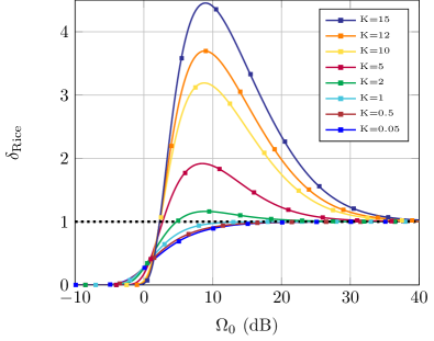
Figure 1: ODO for the Rician fading channel, as a function of the operational average received power $\Omega_{\rm 0}$, for different values of $K$. Solid lines are obtained from (12), markers correspond to Monte Carlo (MC) simulations. The case of the conventional diversity order is included as a reference, using a lightly dotted line.

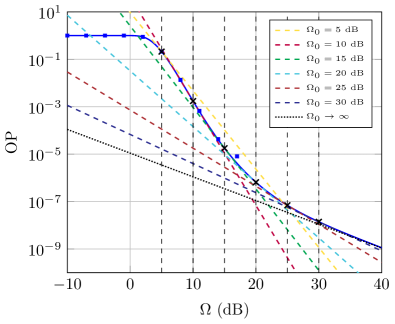
Figure 2: ODO-based linear approximations to the OP for the Rician fading channel at different operational points. Parameter values are $R=1.7$ bps/Hz and $K=15$. Solid lines correspond to the theoretical expression for the OP, markers correspond to MC simulations.

IV-B Effect of a second specular component

Now, let us move to a more general LoS set-up, by assuming the presence of a second dominant specular component. This is encapsulated by Durgin’s TWDP fading model [17], through the parameter $\Delta\in[0,1]$ that captures the amplitude imbalance between these two components. In the limit case of $\Delta=0$, TWDP model reduces to the Rician case, whereas the case with $\Delta=1$ corresponds to a scenario with two LoS components of equal magnitude. Plugging in (9) the PDF and CDF expressions for the TWDP distribution given in [18], we can express

$$\delta_{\rm TWDP}=\left.\frac{W_{\rm th}}{\Omega}\frac{{f}_{\rm g}(W_{\rm th}/\Omega)}{\text{F}_{\rm g}(W_{\rm th}/\Omega)}\right|_{\Omega=\Omega_{\rm 0}},$$ (13)

where

$${f}_{\rm g}(W_{\rm th}/\Omega)= \frac{1}{\pi}\vbox{\hbox{\stretchto[440]{\displaystyle\int}{6ex}}}_{0}^{\pi}{(1+K)}e^{-\kappa_{\theta}-\tfrac{(1+K)W_{\rm th}}{\Omega}}$$

$$\times I_{0}\left(2\sqrt{\tfrac{\kappa_{\theta}(1+K)W_{\rm th}}{\Omega}}\right),$$ (14)

and

$$\text{F}_{\rm g}(W_{\rm th}/\Omega)=1-\tfrac{1}{\pi}\vbox{\hbox{\stretchto[440]{\displaystyle\int}{6ex}}}_{0}^{\pi}\text{Q}_{1}\left(\sqrt{2\kappa_{\theta}};\right.\left.\sqrt{\tfrac{2(1+K)W_{\rm th}}{\Omega}}\right)d\theta.$$ (15)

with $\kappa_{\theta}=K(1+\Delta\cos\theta)$. To better understand the role of $\Delta$ with respect to the Rician case, the ODO is evaluated in Fig. 3 for different values of $\Delta$. A reference scenario with a dominant LoS propagation is assumed, i.e., $K=12$. We note that as $\Delta$ is increased, the ODO is reduced; however, the ODO still offers an improved behavior compared to the conventional diversity order, unless $\Delta\rightarrow 1$. In this situation, often associated to a worse-than-Rayleigh condition [19] due to the probability of cancellation between the dominant specular components, the ODO for the TWDP case is below unity even for such a large value of $K$.

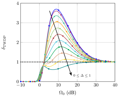
Figure 3: ODO for the TWDP fading channel, as a function of the operational average received power $\Omega_{\rm 0}$, for different values of $\Delta$. Parameter values are $K=12$ and $R=1.7$ bps/Hz. Solid lines are obtained from (13), markers correspond to MC simulations. The case of the conventional diversity order is included as a reference, using a lightly dotted line.

IV-C When conventional diversity order is not applicable

The general definition of diversity order in [5] established a mild condition over the PDF of the SNR, requiring that such a PDF could be approximated by a single polynomial term in the proximity of $0^{+}$. An equivalent condition can be formulated in the Laplace domain, so that the moment generating function (MGF) presents a decay in the form $|s|^{-b}$. However, this condition does not hold in some practical situations, including the case of MIMO keyhole channels with equal number of transmit and receive antennas as a relevant example [10]. Let us focus on the baseline case of a single-input single-output scenario, referred to as product (or cascaded) Rayleigh channel. In this situation, the MGF presents a decay of the form $\log(s)/s$, and the classical diversity order fails to capture the asymptotic behavior of the OP in this scenario. Using the well-known expressions for the cascaded Rayleigh PDF and CDF [8], we can obtain a closed-form expression for the ODO as:

$$\delta_{\rm cas}=\frac{W_{\rm th}}{\Omega_{\rm 0}}\frac{2K_{0}\left(2\sqrt{\tfrac{W_{\rm th}}{\Omega_{\rm 0}}}\right)}{1-2\sqrt{\tfrac{W_{\rm th}}{\Omega_{\rm 0}}}K_{1}\left(2\sqrt{\tfrac{W_{\rm th}}{\Omega_{\rm 0}}}\right)},$$ (16)

where $K_{0}(\cdot)$ and $K_{1}(\cdot)$ correspond to the modified Bessel functions of the second kind and order zero, and one, respectively. The ODO for the cascaded Rayleigh fading channel is represented in Fig. 4, and compared to the case of a single Rayleigh link, which has a simple form given by

$$\delta_{\rm Ray}=\frac{W_{\rm th}}{\Omega_{\rm 0}}\frac{e^{-\tfrac{W_{\rm th}}{\Omega_{\rm 0}}}}{1-e^{-\tfrac{W_{\rm th}}{\Omega_{\rm 0}}}}.$$ (17)

While for the latter the ODO quickly converges to unity, the former has a much slower growth and never manages to achieve the same diversity order as the single Rayleigh link. This is also represented in Fig. 5, where different linear approximations to the log-CDF are represented, using the slope values determined by the ODO. We see that assuming that the cascaded Rayleigh approximately decays with unitary slope may be exceedingly optimistic, and the true decay captured by the ODO must be considered for a proper system design around a given operation point.

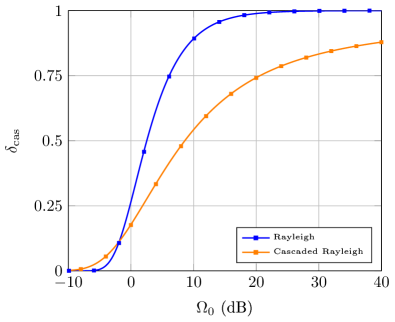
Figure 4: ODO for the cascaded Rayleigh fading channel, as a function of the average SNR $\Omega$. Solid lines are obtained from (16), markers correspond to MC simulations. The case of the single Rayleigh fading channel is included as a reference.

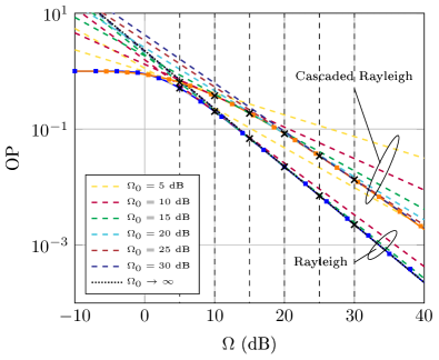
Figure 5: ODO-based linear approximations to the OP for the cascaded Rayleigh fading channel at different operational points. Parameter values are $R=1.7$ bps/Hz. Solid lines correspond to the theoretical expressions for the OP, markers correspond to MC simulations.

V Conclusions

We presented and formally characterized the operational diversity order, as an extension to the classical definition of diversity order but valid for any range of operational SNR. The ODO provides precise information about the decay slope of probability measures for communication systems operating over wireless fading channels, giving insightful information about how power excursions around the system’s SNR can impact its performance. Thanks to the ODO, the increased diversity order offered by LoS propagation is quantified, and the true diversity order in keyhole channels is analytically computed. The simple and compact definition of the ODO in terms of the aggregate fading PDF and CDF opens up the possibility to directly evaluate this insightful performance metric for any wireless system.

Proof of Lemma 1

By analogy with (4), inspection of (5) and (9) implies the following equivalence:

$$\delta=-10\left.\frac{\partial\mathcal{G}\left(x;\Gamma\right)}{\partial x}\right|_{x=x_{\rm 0}}=-10\left.\frac{\partial\log_{10}P_{\rm op}\left(\Omega;\Gamma\right)}{\partial\Omega^{\rm dB}}\right|_{\Omega=\Omega_{\rm 0}},$$ (18)

where the set of parameters $\Gamma$ includes the distribution parameters for $g$ and the threshold value $W_{\rm th}$ for the sake of shorthand notation. To prove the lemma, the following steps are applied from (18):

$$\delta =-\left.\frac{\partial\log_{10}P_{\rm op}\left(\Omega;\Gamma\right)}{\partial\log_{10}\Omega}\right|_{\Omega=\Omega_{\rm 0}},$$ (19)

$$=-\left.\frac{\partial\log P_{\rm op}\left(\Omega;\Gamma\right)}{\partial\log\Omega}\right|_{\Omega=\Omega_{\rm 0}},$$ (20)

$$=-\Omega\left.\frac{\partial\log P_{\rm op}\left(\Omega;\Gamma\right)}{\partial\Omega}\right|_{\Omega=\Omega_{\rm 0}},$$ (21)

$$=-\frac{\Omega}{\text{F}_{g}\left(W_{\rm th}/\Omega\right)}\left.\frac{\partial P_{\rm op}\left(\Omega;\Gamma\right)}{\partial\Omega}\right|_{\Omega=\Omega_{\rm 0}}.$$ (22)

From (2), and applying the chain rule in the integral definition of the OP, we have

$$\left.\frac{\partial P_{\rm op}\left(\Omega;\Gamma\right)}{\partial\Omega}\right|_{\Omega=\Omega_{\rm 0}}=\left.-\frac{W_{\rm th}}{\Omega^{2}}f_{g}\left(W_{\rm th}/\Omega\right)\right|_{\Omega=\Omega_{\rm 0}}.$$ (23)

Finally, combining (22) and (23), the proof is complete.

References

- [1] J. G. Andrews, S. Buzzi, W. Choi, S. V. Hanly, A. Lozano, A. C. K. Soong, and J. C. Zhang, “What Will 5G Be?,” IEEE J. Sel. Areas Commun., vol. 32, pp. 1065–1082, June 2014.
- [2] S. Dang, O. Amin, B. Shihada, and M.-S. Alouini, “What should 6G be?,” Nat. Electron., vol. 3, pp. 20–29, Jan. 2020.
- [3] R. Bahr, “Asymptotic analysis of error probabilities for the nonzero-mean Gaussian hypothesis testing problem,” IEEE Trans. Inf. Theory, vol. 36, pp. 597–607, May 1990.
- [4] J. Ventura-Traveset, G. Caire, E. Biglieri, and G. Taricco, “Impact of diversity reception on fading channels with coded modulation. I. Coherent detection,” IEEE Trans. Commun., vol. 45, pp. 563–572, May 1997.
- [5] Z. Wang and G. Giannakis, “A simple and general parameterization quantifying performance in fading channels,” IEEE Trans. Commun., vol. 51, pp. 1389–1398, Aug. 2003.
- [6] W. K. New, K.-K. Wong, H. Xu, K.-F. Tong, and C.-B. Chae, “Fluid Antenna System: New Insights on Outage Probability and Diversity Gain,” IEEE Trans. Wireless Commun., vol. 23, pp. 128–140, Jan. 2024.
- [7] M. Dohler, R. Heath, A. Lozano, C. Papadias, and R. Valenzuela, “Is the PHY layer dead?,” IEEE Commun. Mag., vol. 49, pp. 159–165, Apr. 2011.
- [8] P. C. F. Eggers, M. Angjelichinoski, and P. Popovski, “Wireless Channel Modeling Perspectives for Ultra-Reliable Communications,” IEEE Trans. Wireless Commun., vol. 18, pp. 2229–2243, Mar. 2019.
- [9] P. Ramírez-Espinosa, R. J. Sánchez-Alarcón, and F. J. López-Martínez, “On the Beneficial Role of a Finite Number of Scatterers for Wireless Physical Layer Security,” IEEE Access, vol. 8, pp. 105055–105064, June 2020.
- [10] S. Sanayei, A. Hedayat, and A. Nosratinia, “Space Time Codes in Keyhole Channels: Analysis and Design,” IEEE Trans. Wireless Commun., vol. 6, pp. 2006–2011, Jan. 2007.
- [11] V. Erceg, S. Fortune, J. Ling, A. Rustako, and R. Valenzuela, “Comparisons of a computer-based propagation prediction tool with experimental data collected in urban microcellular environments,” IEEE J. Sel. Areas Commun., vol. 15, pp. 677–684, May 1997.
- [12] M. Hasna and M.-S. Alouini, “End-to-end performance of transmission systems with relays over Rayleigh-fading channels,” IEEE Trans. Wireless Commun., vol. 2, pp. 1126–1131, Nov. 2003.
- [13] J. D. Griffin and G. D. Durgin, “Gains For RF Tags Using Multiple Antennas,” IEEE Trans. Antennas Propag., vol. 56, pp. 563–570, Feb. 2008.
- [14] M. Safari and M. Uysal, “Cooperative diversity over log-normal fading channels: performance analysis and optimization,” IEEE Trans. Wireless Commun., vol. 7, pp. 1963–1972, May 2008.
- [15] M. Elamassie and M. Uysal, “Incremental Diversity Order for Characterization of FSO Communication Systems Over Lognormal Fading Channels,” IEEE Commun. Lett., vol. 24, pp. 825–829, Feb. 2020.
- [16] R. Narasimhan, “Finite-SNR Diversity–Multiplexing Tradeoff for Correlated Rayleigh and Rician MIMO Channels,” IEEE Trans. Inf. Theory, vol. 52, pp. 3965–3979, Aug. 2006.
- [17] G. Durgin, T. Rappaport, and D. de Wolf, “New analytical models and probability density functions for fading in wireless communications,” IEEE Trans. Commun., vol. 50, pp. 1005–1015, June 2002.
- [18] M. Rao, F. J. Lopez-Martinez, M.-S. Alouini, and A. Goldsmith, “MGF approach to the analysis of generalized two-ray fading models,” IEEE Trans. Wireless Commun., vol. 14, pp. 2548–2561, May 2015.
- [19] D. W. Matolak and J. Frolik, “Worse-than-Rayleigh fading: Experimental results and theoretical models,” IEEE Commun. Mag., vol. 49, no. 4, pp. 140–146, 2011.