Content-based image retrieval for multi-class volumetric radiology images: a benchmark study

Abstract

While content-based image retrieval (CBIR) has been extensively studied in natural image retrieval, its application to medical images presents ongoing challenges, primarily due to the 3D nature of medical images. Recent studies have shown the potential use of pre-trained vision embeddings for CBIR in the context of radiology image retrieval. However, a benchmark for the retrieval of 3D volumetric medical images is still lacking, hindering the ability to objectively evaluate and compare the efficiency of proposed CBIR approaches in medical imaging. In this study, we extend previous work and establish a benchmark for region-based and multi-organ retrieval using the TotalSegmentator dataset (TS) with detailed multi-organ annotations. We benchmark embeddings derived from pre-trained supervised models on medical images against embeddings derived from pre-trained unsupervised models on non-medical images for 29 coarse and 104 detailed anatomical structures in volume and region levels. We adopt a late interaction re-ranking method inspired by text matching for image retrieval, comparing it against the original method proposed for volume and region retrieval achieving retrieval recall of 1.0 for diverse anatomical regions with a wide size range. The findings and methodologies presented in this paper provide essential insights and benchmarks for the development and evaluation of CBIR approaches in the context of medical imaging.

Keywords Content-based image retrieval  $\cdot$ Medical imaging  $\cdot$ Pre-trained embeddings  $\cdot$ Re-ranking

1 Introduction

In the realm of computer vision, content-based image retrieval (CBIR) has been the subject of extensive research for several decades (Dubey, 2021). CBIR systems commonly preserve low-dimensional image representations in a database and subsequently retrieve similar images based on the distance/similarity of the image representations (Khun Jush et al., 2023). Early approaches to CBIR involved manually crafting distinctive features, which led to a semantic gap, resulting in the loss of crucial image details due to the limitations of low-dimensional feature design (Dubey, 2021; Wang et al., 2022). However, recent studies in deep learning have redirected attention towards the creation of machine-generated discriminative feature spaces, effectively addressing and bridging this semantic gap (Qayyum et al., 2017). This shift has significantly enhanced the potential for more accurate and efficient CBIR methods (Dubey, 2021).

While natural image retrieval has been extensively researched, the application of retrieval frameworks to medical images, particularly radiology images, presents ongoing challenges. CBIR offers numerous advantages for medical images. Radiologists can utilize CBIR to search for similar cases, enabling them to review the history, reports, patient diagnoses, and prognoses, thereby enhancing their decision-making process. In real-world use-cases, we often encounter huge unannotated datasets available from different studies where the DICOM headers are removed or incorrect. Finding relevant images in such databases is extremely time-consuming. Moreover, the development of new tools and research in the medical field requires trustable dataset sources and therefore a reliable method for retrieving images, making CBIR an essential component in advancing computer-aided medical image analysis and diagnosis. The challenge with applying CBIR to medical images lies in the fact that algorithms developed for natural images are typically designed for 2D images, while medical images are often 3D volumes which adds a layer of complexity to the retrieval process.

Recent studies have proposed and demonstrated the potential use of pre-trained vision embeddings for CBIR in the context of radiology image retrieval (Khun Jush et al., 2023; Abacha et al., 2023; Denner et al., 2024; Truong et al., 2023). However, these studies have primarily focused on 2D images (Denner et al., 2024) or specific pathologies or tasks (Abacha et al., 2023; Khun Jush et al., 2023; Truong et al., 2023), overlooking the presence of multiple organs in the volumetric images, which is a critical aspect of real-world scenarios. Leveraging multilabel datasets can thoroughly evaluate the efficacy of the proposed methods, enabling a more comprehensive assessment of CBIR approaches for radiology images. Despite previous efforts, there is still no established benchmark available for comparing methods for the retrieval of 3D volumetric medical images. This absence of a benchmark impedes the ability to objectively evaluate and compare the efficiency of the proposed CBIR approaches in the context of medical imaging.

Our previous work (Khun Jush et al., 2023) demonstrated the potential of utilizing pre-trained embeddings, originally trained on natural images, for various medical image retrieval tasks using the Medical Segmentation Decathlon Challenge (MSD) dataset (Antonelli et al., 2022). The approach is outlined in Figure 1. Building upon this, the current study extends the methodology proposed in Khun Jush et al. (2023) to establish a benchmark for anatomical region-based and multi-organ retrieval. While the focus of Khun Jush et al. (2023) was on evaluating sampling methods within the context of the single-organ MSD dataset (Antonelli et al., 2022), it was observed that the single-organ labeling, hinders the evaluations for images containing multiple organs. The main objective of this study is to set a benchmark for organ retrieval at the subvolume or region-based level, which is particularly valuable in practical scenarios, such as when users zoom in on specific regions of interest to retrieve similar images of the precise organ under examination. To achieve this, we evaluate a count-based method in regions using the TotalSegmentator dataset (TS) (Wasserthal et al., 2023). TS dataset along with its detailed multi-organ annotations is a valuable resource for medical image analysis and research. This dataset provides comprehensive annotations for 104 organs or anatomical structures, which allow us to derive fine-grained retrieval tasks and comprehensively evaluate the proposed methods.

The contribution of this work is as follows:

• We benchmarked pre-trained embeddings trained supervised on medical images against pre-trained embeddings trained unsupervised on non-medical images for 29 modified coarse anatomical regions and 104 original anatomical regions from TS dataset Wang et al. (2022).

• We adopted a late interaction re-ranking method originally used for text retrieval called ColBERT (Khattab and Zaharia, 2020) for image retrieval that takes the similarity over the whole volumes into account.

• We benchmarked the re-ranking method against the original method proposed in Khun Jush et al. (2023) for volume and region retrieval on 29 modified coarse anatomical regions and 104 original anatomical regions from TS dataset Wang et al. (2022).

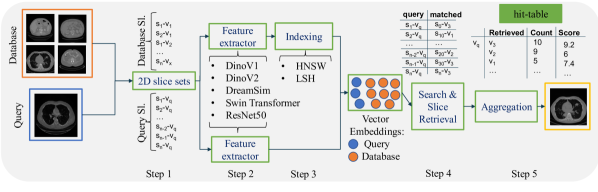
Figure 1: Overview of a retrieval system based on Khun Jush et al. (2023): Step 1: 2D slices are extracted from the 3D volumes. Step 2: Feature extractors are used to extract the embeddings from the database slices and query volumes. Step 3: Database embeddings are indexed using HNSW or LSH indexing. Step 4: Search and slice retrieval is performed, and a hit-table is saved (the hit-table shows the occurrence of volume-ids per each query volume or region saved along with the sum of its total score). Step 5: The results from slice retrieval are aggregated to retrieve the final volume.

2 Materials and Methods

2.1 Vector Database and Indexing

In the context of image search the database is where all the representations of the images, a.k.a. embeddings, and their metadata including annotations are stored. A query allows the user or the system to request specific images in various ways, e.g., by inputting a reference image or a textual description. The goal is to search the database for similar images that match the query. Similarly, in this study, the search process entails comparing a query image with images in the database to identify the most similar image using the similarity of the embeddings. Throughout this process, we do not depend on any metadata information at any stage. Metadata-independence is an intended design choice and in stark contrast to widely used metadata-based image retrieval solutions that frequently lack the necessary specificity in real-world retrieval applications. In small sets, the similarity search is easy but with the growing size of the database, the complexity increases. Accuracy and speed are the key factors in search, thus, naive approaches typically fail in huge datasets.

Indexing in the context of content-based image search involves creating a structured system that allows for efficient storage and retrieval of images based on their visual content. A flat index is the simplest form of indexing, where no modification is made to the vectors before they are used for search. In flat indexing, the query vector is compared to every other full-size vector in the database and their distances are calculated. The nearest k of the searched spaces is then returned as the k-nearest neighbors (kNN). While this method is the most accurate, it comes at the cost of significant search time Aumüller et al. (2020). To improve search time, two approaches can be employed: reducing the vector size through dimensionality reduction, e.g., by reducing the number of bits representing each vector, or reducing the search scope by clustering or organizing vectors into tree structures based on similarity or distance. This results in the identification of an approximation of the true nearest neighbors, known as approximate nearest neighbor search (ANN) (Aumüller et al., 2020).

There are several ANN methods available. Khun Jush et al. (2023) compared Locality Sensitive Hashing (LSH) and Hierarchical Navigable Small World (HNSW) for indexing and search. LSH hashes data points in a way that similar data points are mapped to the same buckets with higher probabilities. This allows for a more efficient search for nearest neighbors by reducing the number of candidates to be examined. HNSW (Malkov and Yashunin, 2018) indexing organizes data into a hierarchical graph structure where each layer of the hierarchy has a lower resolution. The top layer connects data points directly, but the lower layers have fewer connections. The graph structure is designed to allow for efficient navigation during the search. Compared to LSH, HNSW enables faster search and requires less memory Taha et al. (2024). Based on findings in (Khun Jush et al., 2023) HSNW was chosen in this setting over LSH as the preferred indexing method due to speed advantages at a comparable recall.

We propose a system similar to Khun Jush et al. (2023) and Truong et al. (2023) that allows the pre-computation of the image representations of the database. There are various index solutions available to store and search vectors. In this study, we used the Facebook AI Similarity Search (FAISS) package that enables fast similarity search (Johnson et al., 2019). The indexing process involves running the feature extractors on slices of each volumetric image and storing the output embeddings per slice. The produced representations are then added to the search index which is used later on for vector-similarity-based retrieval.

2.2 Feature Extractors

We extend the analysis of Khun Jush et al. (2023) by adding two ResNet50 embeddings and evaluating the performance of six different slice embedding extractors for CBIR tasks. All the feature extractors are based on deep-learning-based models.

Self-supervised Models: We employed three self-supervised models pre-trained on ImageNet (Deng et al., 2009). DINOv1 (Caron et al., 2021), that demonstrated learning efficient image representations from unlabeled data using self-distillation. DINOv2 (Oquab et al., 2023), is built upon DINOv1 (Caron et al., 2021), this model scales the pre-training process by combining an improved training dataset, patchwise objectives during training and introducing a new regularization technique, achieving superior performance on segmentation tasks. DreamSim (Fu et al., 2023), built upon the foundation of DINOv1 (Caron et al., 2021), fine-tunes the model using synthetic data triplets specifically designed to be cognitively impenetrable with human judgments.

Supervised Models: We included a SwinTransformer model (Liu et al., 2021) and a ResNet50 model (He et al., 2016) trained in a supervised manner using the RadImageNet dataset (Mei et al., 2022) that includes 5 million annotated CT, MRI, and ultrasound images of musculoskeletal, neurologic, oncologic, gastrointestinal, endocrine, and pulmonary pathology. Furthermore, a ResNet50 model pre-trained on rendered images of fractal geometries was included based on (Kataoka et al., 2022). These training images are formular-derived, non-natural, and do not require any human annotation.

2.3 Dataset

Table 1: Mapping of the original TS classes to 29 coarse anatomical regions.

Anatomical region	Mapped class	Anatomical region	Mapped class	Anatomical region	Mapped class
adrenal gland left	adrenal gland	iliopsoas right	iliopsoas	rib right 8	rib
adrenal gland right	adrenal gland	inferior vena cava	cardiovascular system	rib right 9	rib
aorta	cardiovascular system	kidney left	kidney	sacrum	sacrum
autochthon left	autochthon	kidney right	kidney	scapula left	scapula
autochthon right	autochthon	liver	liver	scapula right	scapula
brain	brain	lung lower lobe left	lung	small bowel	small bowel
clavicula left	clavicula	lung lower lobe right	lung	spleen	spleen
clavicula right	clavicula	lung middle lobe right	lung	stomach	stomach
colon	colon	lung upper lobe left	lung	trachea	trachea
duodenum	duodenum	lung upper lobe right	lung	urinary bladder	urinary bladder
esophagus	esophagus	pancreas	pancreas	vertebrae C1	vertebrae
face	face	portal and splenic vein	portal & splenic vein	vertebrae C2	vertebrae
femur left	femur	pulmonary artery	cardiovascular system	vertebrae C3	vertebrae
femur right	femur	rib left 1	rib	vertebrae C4	vertebrae
gallbladder	gallbladder	rib left 10	rib	vertebrae C5	vertebrae
gluteus maximus left	gluteus muscles	rib left 11	rib	vertebrae C6	vertebrae
gluteus maximus right	gluteus muscles	rib left 12	rib	vertebrae C7	vertebrae
gluteus medius left	gluteus muscles	rib left 2	rib	vertebrae L1	vertebrae
gluteus medius right	gluteus muscles	rib left 3	rib	vertebrae L2	vertebrae
gluteus minimus left	gluteus muscles	rib left 4	rib	vertebrae L3	vertebrae
gluteus minimus right	gluteus muscles	rib left 5	rib	vertebrae L4	vertebrae
heart atrium left	cardiovascular system	rib left 6	rib	vertebrae L5	vertebrae
heart atrium right	cardiovascular system	rib left 7	rib	vertebrae T1	vertebrae
heart myocardium	cardiovascular system	rib left 8	rib	vertebrae T10	vertebrae
heart ventricle left	cardiovascular system	rib left 9	rib	vertebrae T11	vertebrae
heart ventricle right	cardiovascular system	rib right 1	rib	vertebrae T12	vertebrae
hip left	hip	rib right 10	rib	vertebrae T2	vertebrae
hip right	hip	rib right 11	rib	vertebrae T3	vertebrae
humerus left	humerus	rib right 12	rib	vertebrae T4	vertebrae
humerus right	humerus	rib right 2	rib	vertebrae T5	vertebrae
iliac artery left	cardiovascular system	rib right 3	rib	vertebrae T6	vertebrae
iliac artery right	cardiovascular system	rib right 4	rib	vertebrae T7	vertebrae
iliac vena left	cardiovascular system	rib right 5	rib	vertebrae T8	vertebrae
iliac vena right	cardiovascular system	rib right 6	rib	vertebrae T9	vertebrae
iliopsoas left	iliopsoas	rib right 7	rib

We designed a CBIR benchmark relying on the TS dataset which is publicly available on Wasserthal et al. (2023). TS is a dataset comprising 1204 computed tomography (CT) volumes with 104 anatomical structure annotations. Since the anatomical regions presented in the original dataset include small structures we additionally mapped these small regions to classes with coarse labels, e.g., all the rib classes are mapped to a single class in the coarse label classes. The coarse label classes can provide insight into the retrieval of anatomical regions that are close to the target organ. LABEL:tab:_mapping_table shows the mapping of the TS original classes to the coarse classes. The query cases are sourced from the test split, while the train set serves as the database for searching. The search is assessed on the retrieval rate of 29 coarse anatomical structures and 104 original TS anatomical structures.

The models presented in Section 2.2 are 2D models used without fine-tuning to extract the embeddings. Thus, per each 3D volume, individual 2D slices of the corresponding 3D volumes are utilized for embedding extraction. The input size for all the used models is equal to $224\times 224$ pixels with image replication along the RGB channel axis. For all the ViT-based models and the ResNet50 trained on fractal images, images are normalized to the ImageNet mean and standard deviation of $(.485,.456,.406)$ and $(.229,.224,.225)$, respectively. For the SwinTransformer and the ResNet50 model pre-trained on the RadImageNet dataset, the images are normalized to $.5$ mean and $.5$ standard deviation based on Mei et al. (2022). The total size of the database is $290757$ embeddings, while the final query set of the test set comprises $20442$ embeddings.

2.4 Search and Retrieval

After creating the vector database, the search is performed using the embeddings extracted from slices of query volumes. The simplest way of retrieval is to match each 2D slice with the most similar 2D slice in the database. Here, we used cosine similarity. In Khun Jush et al. (2023) we introduced this method as the lower bound baseline for evaluating our proposed aggregation and sampling schemes. Similarly, in this work, we keep the slice-wise evaluation as the lower bound for the retrieval rate of our methods. We performed and evaluated image retrieval at the level of volumes and sub-volumes or regions. The difference between volume and region-based retrieval is as follows:

2.4.1 Volume-based

For every slice within the query volume, the system retrieves the most similar slice from the database. Subsequently, the corresponding volume-id and its similarity score for each retrieved slice are stored in a hit-table similar to the hit-table shown in Figure 1. The aggregation method in Khun Jush et al. (2023) is a count-based method that retrieves per query volume the volume that has the most number of similar slices from the database Figure 1. Abacha et al. (2023) refers to this method as the evaluation based on frequency. For every retrieved slice, its corresponding volume-id is saved in the hit-table. The occurrence of volume-ids is then counted per each query volume. The volume with the highest count is selected as the most similar retrieved volume. Evaluation is then carried out based on the aggregated labels of the query volume and the most similar retrieved volume. This method retrieves the most similar volume per query volume. An overview is shown in Figure 2(a).

2.4.2 Region-based

The hit-table is generated following the process outlined in Section 2.4.1 with the same aggregation method. The key distinction lies in the fact that the subsequent retrieved volumes and final evaluation are predicated upon sub-volumes or anatomical regions. Meaning, that the occurrence of volume-ids is counted per each query region. The volumes with the highest count are selected as the most similar retrieved volumes. This means that in contrast to volume-based retrieval when all organs are under examination, multiple volumes are retrieved for each query volume. Naturally, only one organ can be searched (by querying only the slices that contain the limited organ view). The overview of this method is depicted in Figure 2(b).

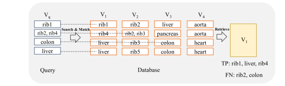
(a)

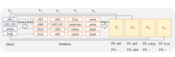
(b)

Figure 2: Comparison of volume-based (a) and region-based (b) retrieval, in volume-based retrieval per each query volume one volume is retrieved while in region-based retrieval per each anatomical structure, one volume is retrieved.

2.5 Re-ranking

Re-ranking in information retrieval involves the process of re-ordering the initially retrieved results to better align with the user’s information needs. This can be achieved through different methods such as relevance feedback, learning to rank algorithms, or incorporating contextual information (Ai et al., 2018; Guo et al., 2020; MacAvaney et al., 2019). Relevance feedback allows users to provide input on the initial results, which is then used to adjust the ranking (Ai et al., 2018). Learning to rank algorithms utilize machine learning techniques to re-rank results based on relevant features (Guo et al., 2020). Additionally, re-ranking methods may also consider contextual information such as user behavior, temporal relevance, or other relevant factors to better reflect the user’s current information needs, ultimately enhancing the overall quality of retrieved results (MacAvaney et al., 2019). A method based on contextualized information proposed in Khattab and Zaharia (2020) called ColBERT (Contextualized Late Interaction over BERT). ColBERT operates by generating contextualized representations of the query and the documents using BERT (Devlin et al., 2018). In this method, queries and documents are encoded into more detailed multi-vector representations, and relevance is gauged through comprehensive yet scalable interactions between these sets of vectors. ColBERT creates an embedding for each token in the query and document, and it measures relevance as the total of maximum similarities between each query vector and all vectors within the document (Santhanam et al., 2021). This late interaction approach allows for a more refined and contextually aware retrieval process, thereby enhancing the quality of information retrieval.

Inspired by ColBERT we introduce a method in which filtering of the search space is performed and the total similarity of the entire target volume is considered to re-rank and score the retrieved volumes. To create an analogy to the ColBERT method each word can be considered as one slice and each passage of the database or each question of the query can be considered as one volume. Instead of the BERT encoder for the image retrieval task, the pre-trained vision models can be used to create the embeddings as discussed in Section 2.2.

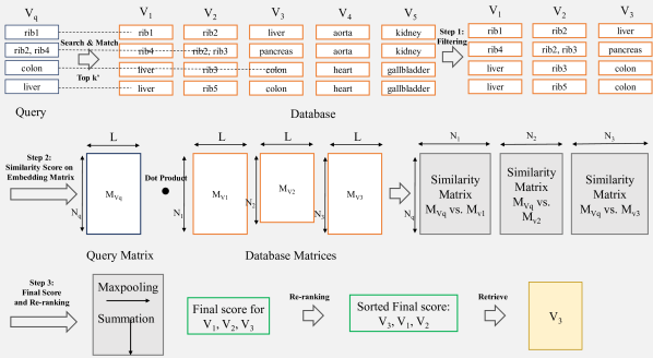
Figure 3: Overview of re-ranking: Step 1: Filtering based on at least one similar slice leads to the selection of candidate volumes Step 2: followed by similarity score computation using dot product on the normalized embedding matrices. Step 3: The final step involves max-pooling and summation to determine the top-scoring volumes for retrieval.

An overview of the proposed method is shown in Figure 3. The method consists of the following steps:

2.5.1 Step 1: Filtering

In the first step per each slice query, top k’ retrieval in the indexed space is performed based on cosine, L2 similarity, etc. In this step all the embedding are saved as vectors, one per each slice both for the query and the database. For each volume, that contained $N_{q}$ slices, maximum $N_{q}\times k^{\prime}$ volumes are retrieved. Thus, for $V$ query volumes or regions, in total maximum $N_{q}\times k^{\prime}\times V$ volumes are filtered. In the filtered volumes there is at least one slice that has a high similarity with its corresponding query volume or region. all the following operations are performed on the subsection of the filtered volumes and the re-ranking will be performed only on the filtered volumes.

2.5.2 Step 2: Similarity Score on Embedding Matrix

In this step, volumes are treated as matrices, where for each query $V_{q}$ there is a matrix of multiple embeddings. If the embeddings per slice have size $L$ and $N_{q}$ is the number of slices the loaded query matrix $M_{V_{q}}$ has size $Nq\times L$. Similarly, there is a matrix of multiple embeddings for each volume in the database. In this step, all the embeddings should be normalized such that the L2 norm is equal to 1. The result is that the dot-product of any two embeddings will be equivalent to their cosine similarity. The dot product of each query embedding matrix with size $Nq\times L$ to an embedding matrix of a volume in the database of size $M_{v_{x}}\times L$ results in a similarity score matrix of size $N_{q}\times M_{v_{x}}$ where $x=1,2,...$ denoting volume-id number.

2.5.3 Step 3: Final Score and Re-ranking

To compute the score of each volume, its dimension across the volume is reduced via max-pooling (i.e. representing the most similar slice in the target volume for each query slice). Across the query dimension, a summation is performed (i.e. representing the total score of the similarity of all the slices of the query to the whole volume in the database). Finally, the k’ documents are sorted by their total scores, and the volume/volumes with the maximum overall score are retrieved.

3 Evaluation

In this section, we evaluate the retrieval recall of the methods explained in Section 2.4 and Section 2.5. Since finding extra anatomical regions is not critical for this study (that would be the anatomical regions that are present in the retrieved volume/slice and are missing from the query volume/slice, i.e. false positives (FP)) we do not discuss the precision metric. The results are presented for 29 anatomical structures presented in LABEL:tab:_mapping_table and 104 anatomical structures that were originally presented in Wasserthal et al. (2023). In the tables presented in this section, the average and standard deviation (STD) columns are aimed to highlight difficult classes across models (low average) and the ones that have higher variations among models (higher STD). The average and STD rows show the average and STD over all the classes for each model.

3.1 Search and Retrieval

3.1.1 Slice-wise

In the computation of slice-wise recall, per each slice, if the retrieved slice contains the same anatomical region/regions the corresponding class/classes are considered as the true positive class (TP). If the query slice contains anatomical regions that are not present in the retrieved slice that class is considered a false negative (FN).

LABEL:tab:slicewise-recall-28-regions and LABEL:tab:slicewise-recall-104-regions show the retrieval recall of 29 coarse anatomical regions and 104 original TS anatomical regions, respectively, using the slice-wise method (lower bound).

In slice-wise retrieval, DreamSim is the best-performing model with retrieval recall of $.849\pm.148$ and $.797\pm.129$ for coarse and original TS classes, respectively. ResNet50 pre-trained on fractal images has the lowest retrieval recall almost on every anatomical region for 29 and 104 classes. This is however expected due to the nature of synthetic generated images.

In LABEL:tab:slicewise-recall-104-regions the gallbladder has the lowest retrieval rate followed by vertebrae C4 and C5 (see average column). However, in LABEL:tab:slicewise-recall-28-regions the vertebrae class shows a higher recall which indicated that the vertebrae classes were detected but the exact location, i.e. C4 or C5 were mismatched. The same pattern can be observed in rib classes.

Table 2: Slice-wise recall of coarse anatomical regions (29 classes) using HNSW Indexing. In each row, bold numbers represent the best-performing values, while italicized numbers indicate the worst-performing. The separate average and standard deviation (STD) columns are color-coded, with blue indicating the best-performing values and yellow indicating the worst-performing values across different models. Additionally, bold numbers in colored columns represent the best classes in terms of average and standard deviation, while italicized values represent the worst-performing class across the models.

Model	DINOv1	DINOv2	DreamSim	SwinTrans.	ResNet50
Dataset (pre-trained)	(ImgNet)	(ImgNet)	(ImgNet)	(RadImg)	(Fractaldb)	(RadImg)	Average	STD
adrenal gland	.749	.639	.671	.614	.490	.557	.620	.090
autochthon	.980	.974	.979	.976	.941	.965	.969	.015
brain	.852	.843	.901	.894	.850	.863	.867	.025
cardiovascular system	.978	.974	.979	.970	.941	.953	.966	.015
clavicula	.886	.884	.898	.857	.632	.873	.838	.102
colon	.932	.931	.945	.912	.830	.905	.909	.042
duodenum	.678	.682	.719	.697	.605	.733	.686	.045
esophagus	.934	.934	.936	.933	.870	.894	.917	.028
face	.854	.840	.872	.788	.692	.733	.797	.072
femur	.927	.907	.953	.914	.778	.860	.890	.063
gallbladder	.246	.345	.312	.341	.347	.400	.332	.051
gluteus muscles	.964	.940	.978	.950	.879	.915	.938	.036
hip	.959	.928	.974	.941	.880	.907	.931	.034
humerus	.575	.600	.633	.598	.351	.523	.547	.102
iliopsoas	.950	.933	.957	.934	.863	.923	.927	.034
kidney	.759	.771	.791	.776	.641	.776	.752	.055
liver	.840	.817	.844	.841	.814	.839	.833	.013
lung	.953	.930	.958	.940	.890	.898	.928	.028
pancreas	.720	.685	.779	.734	.552	.722	.699	.078
portal and splenic vein	.731	.627	.679	.658	.522	.584	.634	.074
rib	.950	.942	.951	.948	.900	.933	.937	.020
sacrum	.894	.865	.907	.878	.805	.856	.867	.036
scapula	.935	.913	.924	.891	.793	.869	.887	.052
small bowel	.896	.872	.900	.894	.783	.892	.873	.045
spleen	.774	.719	.735	.699	.731	.693	.725	.029
stomach	.811	.781	.844	.778	.741	.752	.784	.038
trachea	.893	.862	.903	.863	.762	.816	.850	.053
urinary bladder	.720	.643	.722	.720	.633	.666	.684	.041
vertebrae	.981	.967	.977	.969	.950	.964	.968	.011
Average	.855	.832	.863	.837	.751	.813
STD	.108	.118	.107	.114	.152	.124

Table 3: Slice-wise recall of all TS anatomical regions (104 classes) using HNSW Indexing. In each row, bold numbers represent the best-performing values, while italicized numbers indicate the worst-performing. The separate average and standard deviation (STD) columns are color-coded, with blue indicating the best-performing values and yellow indicating the worst-performing values across different models. Additionally, bold numbers in colored columns represent the best classes in terms of average and standard deviation, while italicized values represent the worst-performing class across the models.

Model	DINOv1	DINOv2	DreamSim	SwinTrans.	ResNet50
Dataset (pre-trained)	(ImgNet)	(ImgNet)	(ImgNet)	(RadImg)	(Fractaldb)	(RadImg)	Average	STD
adrenal gland left	.636	.524	.573	.539	.407	.453	.522	.082
adrenal gland right	.644	.515	.593	.551	.408	.521	.539	.080
aorta	.954	.941	.946	.952	.915	.926	.939	.015
autochthon left	.981	.972	.980	.974	.942	.966	.969	.014
autochthon right	.980	.974	.979	.976	.942	.965	.969	.014
brain	.852	.843	.901	.894	.850	.863	.867	.025
clavicula left	.866	.875	.886	.864	.636	.874	.833	.097
clavicula right	.862	.871	.867	.840	.614	.855	.818	.101
colon	.932	.931	.945	.912	.830	.905	.909	.042
duodenum	.678	.682	.719	.697	.605	.733	.686	.045
esophagus	.934	.934	.936	.933	.870	.894	.917	.028
face	.854	.840	.872	.788	.692	.733	.797	.072
femur left	.920	.902	.940	.909	.773	.855	.883	.061
femur right	.931	.910	.952	.938	.808	.915	.909	.052
gallbladder	.246	.345	.312	.341	.347	.400	.332	.051
gluteus maximus left	.937	.914	.951	.927	.845	.903	.913	.037
gluteus maximus right	.942	.914	.945	.925	.858	.900	.914	.032
gluteus medius left	.930	.878	.948	.920	.824	.883	.897	.045
gluteus medius right	.922	.892	.951	.923	.852	.893	.905	.034
gluteus minimus left	.872	.824	.894	.855	.795	.876	.853	.037
gluteus minimus right	.876	.811	.878	.874	.819	.898	.860	.035
heart atrium left	.709	.656	.800	.680	.588	.542	.663	.091
heart atrium right	.793	.762	.870	.773	.684	.668	.758	.074
heart myocardium	.798	.757	.844	.808	.715	.733	.776	.049
heart ventricle left	.778	.724	.824	.788	.699	.720	.756	.048
heart ventricle right	.802	.801	.851	.822	.723	.738	.789	.049
hip left	.959	.928	.971	.937	.880	.905	.930	.034
hip right	.963	.932	.977	.948	.889	.916	.938	.032
humerus left	.525	.571	.591	.577	.313	.471	.508	.105
humerus right	.593	.625	.627	.567	.314	.529	.543	.118
iliac artery left	.882	.863	.902	.893	.813	.841	.866	.034
iliac artery right	.905	.869	.918	.895	.822	.851	.876	.036
iliac vena left	.903	.868	.908	.893	.825	.857	.876	.032
iliac vena right	.910	.870	.923	.891	.831	.873	.883	.033
iliopsoas left	.950	.929	.958	.932	.861	.924	.926	.034
iliopsoas right	.947	.929	.951	.932	.854	.922	.923	.035
inferior vena cava	.928	.896	.922	.923	.841	.893	.901	.033
kidney left	.719	.708	.762	.747	.600	.762	.716	.061
kidney right	.708	.724	.755	.737	.602	.756	.714	.058
liver	.840	.817	.844	.841	.814	.839	.833	.013
lung lower lobe left	.903	.885	.908	.887	.826	.811	.870	.041
lung lower lobe right	.903	.880	.914	.897	.806	.809	.868	.048
lung middle lobe right	.800	.785	.818	.794	.726	.699	.770	.047
lung upper lobe left	.917	.909	.921	.906	.850	.875	.896	.028
lung upper lobe right	.928	.883	.919	.885	.818	.848	.880	.042
pancreas	.720	.685	.779	.734	.552	.722	.699	.078
portal and splenic vein	.731	.627	.679	.658	.522	.584	.634	.074
pulmonary artery	.819	.711	.773	.679	.526	.563	.679	.115
rib left 1	.855	.824	.867	.851	.669	.821	.815	.073
rib left 10	.827	.775	.803	.823	.742	.747	.786	.037
rib left 11	.773	.767	.785	.788	.694	.756	.761	.034
rib left 12	.594	.568	.682	.620	.481	.576	.587	.066
rib left 2	.841	.804	.858	.807	.681	.803	.799	.062
rib left 3	.832	.803	.808	.805	.728	.789	.794	.035
rib left 4	.820	.783	.809	.776	.738	.759	.781	.031
rib left 5	.789	.786	.805	.784	.699	.723	.764	.043
rib left 6	.815	.787	.797	.787	.706	.751	.774	.039
rib left 7	.830	.825	.834	.829	.734	.778	.805	.040
rib left 8	.810	.799	.850	.831	.745	.777	.802	.038
rib left 9	.826	.803	.833	.853	.737	.780	.805	.042
rib right 1	.852	.820	.828	.831	.672	.827	.805	.066
rib right 10	.827	.768	.804	.814	.728	.747	.781	.040
rib right 11	.770	.763	.798	.771	.681	.742	.754	.040
rib right 12	.577	.570	.619	.634	.456	.556	.569	.063
rib right 2	.839	.820	.840	.815	.680	.802	.799	.060
rib right 3	.850	.794	.826	.795	.725	.780	.795	.043
rib right 4	.834	.790	.809	.770	.738	.753	.782	.036
rib right 5	.802	.791	.810	.776	.709	.718	.768	.044
rib right 6	.810	.788	.772	.779	.709	.741	.766	.036
rib right 7	.803	.813	.805	.817	.731	.765	.789	.034
rib right 8	.814	.792	.847	.833	.754	.778	.803	.035
rib right 9	.823	.793	.813	.844	.738	.776	.798	.038
sacrum	.894	.865	.907	.878	.805	.856	.867	.036
scapula left	.922	.891	.908	.891	.798	.884	.882	.044
scapula right	.930	.905	.919	.884	.799	.872	.885	.047
small bowel	.896	.872	.900	.894	.783	.892	.873	.045
spleen	.774	.719	.735	.699	.731	.693	.725	.029
stomach	.811	.781	.844	.778	.741	.752	.784	.038
trachea	.893	.862	.903	.863	.762	.816	.850	.053
urinary bladder	.720	.643	.722	.720	.633	.666	.684	.041
vertebrae C1	.555	.571	.655	.592	.399	.592	.561	.086
vertebrae C2	.744	.613	.812	.594	.529	.643	.656	.104
vertebrae C3	.677	.566	.586	.414	.271	.359	.479	.155
vertebrae C4	.427	.377	.519	.488	.323	.308	.407	.087
vertebrae C5	.513	.444	.572	.565	.330	.366	.465	.102
vertebrae C6	.562	.562	.536	.423	.220	.445	.458	.131
vertebrae C7	.712	.645	.685	.576	.375	.580	.595	.121
vertebrae L1	.620	.561	.662	.653	.452	.540	.582	.080
vertebrae L2	.555	.514	.658	.587	.411	.591	.553	.084
vertebrae L3	.747	.533	.608	.593	.503	.629	.602	.086
vertebrae L4	.612	.449	.639	.693	.523	.572	.581	.087
vertebrae L5	.732	.592	.748	.714	.606	.631	.670	.069
vertebrae T1	.723	.698	.704	.689	.464	.694	.662	.098
vertebrae T10	.568	.517	.583	.565	.449	.518	.533	.050
vertebrae T11	.555	.539	.574	.546	.433	.506	.526	.051
vertebrae T12	.556	.554	.604	.581	.468	.562	.554	.047
vertebrae T2	.750	.670	.752	.726	.563	.679	.690	.071
vertebrae T3	.794	.744	.814	.736	.621	.668	.729	.073
vertebrae T4	.742	.715	.713	.666	.540	.666	.674	.072
vertebrae T5	.647	.618	.701	.627	.513	.550	.609	.068
vertebrae T6	.696	.627	.637	.597	.488	.514	.593	.079
vertebrae T7	.703	.680	.705	.613	.460	.516	.613	.104
vertebrae T8	.595	.590	.728	.564	.450	.469	.566	.101
vertebrae T9	.603	.540	.660	.609	.515	.524	.575	.057
Average	.784	.750	.797	.765	.659	.726
STD	.137	.144	.129	.140	.172	.154

3.1.2 Volume-based

This section presents the recall of volume-based retrieval explained in Section 2.4.1 An overview of the evaluation is shown in Figure 2(a). In volume-based retrieval, per each query volume, one volume is retrieved. In the recall computation, the classes present in both the query and the retrieved volume are considered TP classes. The classes that are present in the query volume and are missing from the retrieved volume are considered FN.

LABEL:tab:volumewise-recall-29-regions and LABEL:tab:volumewise-recall-104-regions present the retrieval recall of the volume-based method on 29 and 104 classes, respectively. The overall recall rates are increased compared slice-wise which is expected due to the aggregation and effects of neighboring slices.

LABEL:tab:volumewise-recall-29-regions shows that ResNet50 trained on RadImageNet outperforms other methods with an average recall of $.952\pm.043$. However, in LABEL:tab:volumewise-recall-104-regions DINOv1 outperforms all models including ResNet50 with an average recall of $.923\pm.077$. This shows that the embeddings of finer classes are retrieved and assigned to a different similar class by ResNet50, thus, the performance from fine to coarse classes is improved. Whereas, all the self-supervised methods in LABEL:tab:volumewise-recall-104-regions outperform the supervised methods. Although some models perform slightly better than others based on looking at isolated classes, overall models perform on par.

Table 4: Volume-based retrieval recall of coarse anatomical regions (29 classes) using HNSW Indexing. In each row, bold numbers represent the best-performing values, while italicized numbers indicate the worst-performing. The separate average and standard deviation (STD) columns are color-coded, with blue indicating the best-performing values and yellow indicating the worst-performing values across different models. Additionally, bold numbers in colored columns represent the best classes in terms of average and standard deviation, while italicized values represent the worst-performing class across the models.

Model	DINOv1	DINOv2	DreamSim	SwinTrans.	ResNet50
Dataset (pre-trained)	(ImgNet)	(ImgNet)	(ImgNet)	(RadImg)	(Fractaldb)	(RadImg)	Average	STD
adrenal gland	1.000	.960	.960	.960	.980	.980	.973	.016
autochthon	.985	.969	.969	.985	.985	1.000	.982	.012
brain	.692	.769	.769	.846	.769	.846	.782	.058
cardiovascular system	1.000	1.000	.968	1.000	1.000	.968	.989	.016
clavicula	.949	.949	.949	.897	.821	.949	.919	.052
colon	1.000	.943	.981	.943	1.000	.962	.972	.026
duodenum	.940	.860	.900	.920	.980	.920	.920	.040
esophagus	.964	.964	.946	.982	.946	1.000	.967	.021
face	.765	.765	.706	.706	.706	.882	.755	.069
femur	.933	.933	.911	.911	.956	.933	.930	.017
gallbladder	.846	.795	.872	.821	.846	.897	.846	.036
gluteus muscles	1.000	.977	.977	.977	1.000	.955	.981	.017
hip	1.000	.977	.977	.977	1.000	.955	.981	.017
humerus	.898	.857	.980	.898	.878	.878	.898	.043
iliopsoas	.981	.981	.962	.962	.981	.962	.972	.010
kidney	.945	.927	.945	.891	.927	.964	.933	.025
liver	.964	.945	.982	.945	.982	.982	.967	.018
lung	.983	.983	.931	.983	.983	.983	.974	.021
pancreas	.940	.920	.920	.940	.960	.980	.943	.023
portal and splenic vein	.980	.960	.940	.980	.960	.980	.967	.016
rib	.983	.983	.949	1.000	.966	1.000	.980	.020
sacrum	.977	.955	.977	.955	1.000	.955	.970	.019
scapula	.909	.909	.909	.818	.886	.886	.886	.035
small bowel	.958	.896	.917	.958	.979	.938	.941	.031
spleen	1.000	.980	.960	.980	.980	1.000	.983	.015
stomach	1.000	.980	.961	.980	.980	1.000	.984	.015
trachea	.951	.951	.951	.878	.805	.902	.907	.059
urinary bladder	1.000	.977	.977	.953	.977	.953	.973	.018
vertebrae	.984	.969	1.000	.984	1.000	1.000	.990	.013
Average	.949	.932	.936	.932	.939	.952
STD	.072	.064	.063	.067	.078	.043

Table 5: Volume-based retrieval recall of all TS anatomical regions (104 classes) using HNSW Indexing. In each row, bold numbers represent the best-performing values, while italicized numbers indicate the worst-performing. The separate average and standard deviation (STD) columns are color-coded, with blue indicating the best-performing values and yellow indicating the worst-performing values across different models. Additionally, bold numbers in colored columns represent the best classes in terms of average and standard deviation, while italicized values represent the worst-performing class across the models.

Model	DINOv1	DINOv2	DreamSim	SwinTrans.	ResNet50
Dataset (pre-trained)	(ImgNet)	(ImgNet)	(ImgNet)	(RadImg)	(Fractaldb)	(RadImg)	Average	STD
adrenal gland left	.960	.900	.920	.900	.900	.960	.923	.029
adrenal gland right	.980	.900	.940	.900	.900	.960	.930	.035
aorta	.984	.934	.934	.934	.918	.934	.940	.022
autochthon left	.969	.923	.938	.923	.908	.954	.936	.023
autochthon right	.969	.923	.938	.923	.908	.954	.936	.023
brain	.692	.692	.692	.692	.769	.692	.705	.031
clavicula left	.949	.923	.897	.821	.821	.897	.885	.053
clavicula right	.974	.947	.921	.816	.816	.895	.895	.067
colon	.981	.906	.962	.906	.906	.925	.931	.033
duodenum	.920	.820	.880	.880	.880	.880	.877	.032
esophagus	.946	.911	.911	.911	.875	.964	.920	.031
face	.765	.706	.647	.588	.706	.765	.696	.069
femur left	.911	.911	.889	.867	.867	.911	.893	.022
femur right	.927	.927	.902	.902	.927	.927	.919	.013
gallbladder	.846	.744	.846	.795	.795	.872	.816	.047
gluteus maximus left	.977	.953	.953	.907	.930	.930	.942	.024
gluteus maximus right	.977	.953	.930	.930	.907	.930	.938	.024
gluteus medius left	.977	.932	.955	.909	.909	.932	.936	.027
gluteus medius right	.977	.930	.953	.930	.907	.953	.942	.024
gluteus minimus left	.977	.953	.953	.907	.930	.930	.942	.024
gluteus minimus right	.976	.952	.952	.905	.929	.952	.944	.025
heart atrium left	.915	.830	.872	.936	.830	.979	.894	.060
heart atrium right	.939	.898	.898	.939	.816	.980	.912	.056
heart myocardium	.939	.898	.898	.939	.816	.980	.912	.056
heart ventricle left	.939	.898	.878	.939	.816	.980	.908	.057
heart ventricle right	.939	.898	.898	.939	.816	.980	.912	.056
hip left	.977	.932	.955	.932	.909	.932	.939	.023
hip right	.977	.932	.955	.932	.886	.932	.936	.030
humerus left	.949	.897	.949	.872	.846	.897	.902	.041
humerus right	.875	.854	.917	.833	.833	.813	.854	.037
iliac artery left	.977	.932	.955	.932	.909	.955	.943	.024
iliac artery right	.955	.909	.932	.909	.886	.932	.920	.024
iliac vena left	.977	.932	.955	.932	.909	.932	.939	.023
iliac vena right	.955	.909	.932	.909	.886	.932	.920	.024
iliopsoas left	.943	.887	.925	.925	.906	.925	.918	.019
iliopsoas right	.961	.922	.941	.922	.902	.941	.931	.021
inferior vena cava	.982	.930	.965	.930	.912	.965	.947	.027
kidney left	.906	.887	.906	.849	.868	.943	.893	.033
kidney right	.900	.820	.880	.860	.820	.900	.863	.037
liver	.945	.909	.964	.909	.891	.945	.927	.028
lung lower lobe left	.912	.877	.842	.895	.895	.912	.889	.026
lung lower lobe right	.946	.911	.875	.893	.875	.929	.905	.029
lung middle lobe right	.939	.918	.878	.959	.837	.980	.918	.053
lung upper lobe left	.929	.911	.911	.911	.839	.946	.908	.036
lung upper lobe right	.891	.870	.870	.804	.891	.870	.866	.032
pancreas	.920	.880	.900	.900	.900	.960	.910	.028
portal and splenic vein	.960	.920	.920	.940	.880	.960	.930	.030
pulmonary artery	.850	.825	.850	.750	.800	.800	.813	.038
rib left 1	.974	.947	.921	.842	.816	.895	.899	.061
rib left 10	.961	.922	.922	.941	.882	.980	.935	.034
rib left 11	.961	.922	.922	.941	.882	.980	.935	.034
rib left 12	.896	.938	.896	.917	.875	.958	.913	.031
rib left 2	.950	.950	.925	.825	.825	.875	.892	.058
rib left 3	.951	.927	.927	.829	.854	.878	.894	.048
rib left 4	.900	.875	.900	.825	.850	.875	.871	.029
rib left 5	.909	.841	.864	.864	.841	.909	.871	.031
rib left 6	.880	.840	.860	.940	.820	.960	.883	.056
rib left 7	.959	.918	.918	.959	.857	.980	.932	.044
rib left 8	.961	.922	.922	.961	.882	.980	.938	.036
rib left 9	.961	.922	.922	.961	.902	.980	.941	.030
rib right 1	.974	.947	.921	.842	.842	.895	.904	.054
rib right 10	.961	.922	.922	.941	.882	.980	.935	.034
rib right 11	.961	.922	.922	.941	.882	.980	.935	.034
rib right 12	.872	.915	.872	.936	.830	.957	.897	.047
rib right 2	.974	.949	.923	.846	.846	.897	.906	.053
rib right 3	.927	.902	.902	.805	.854	.854	.874	.045
rib right 4	.927	.902	.878	.829	.854	.854	.874	.036
rib right 5	.932	.841	.864	.864	.864	.886	.875	.031
rib right 6	.918	.857	.857	.918	.796	.918	.878	.050
rib right 7	.959	.918	.918	.959	.816	.980	.925	.059
rib right 8	.961	.922	.922	.961	.882	.980	.938	.036
rib right 9	.941	.902	.902	.941	.902	.961	.925	.026
sacrum	.955	.909	.955	.909	.909	.932	.928	.022
scapula left	.902	.878	.902	.780	.854	.854	.862	.045
scapula right	.930	.884	.884	.767	.860	.860	.864	.054
small bowel	.938	.854	.896	.917	.896	.896	.899	.028
spleen	.980	.940	.940	.940	.900	.980	.947	.030
stomach	.980	.941	.941	.941	.902	.980	.948	.030
trachea	.951	.927	.902	.805	.805	.854	.874	.063
urinary bladder	.977	.953	.953	.907	.907	.930	.938	.028
vertebrae C1	.643	.643	.643	.643	.714	.643	.655	.029
vertebrae C2	.692	.692	.692	.692	.769	.692	.705	.031
vertebrae C3	.643	.714	.571	.714	.857	.714	.702	.095
vertebrae C4	.600	.667	.533	.667	.867	.667	.667	.112
vertebrae C5	.650	.600	.600	.500	.700	.600	.608	.066
vertebrae C6	.818	.758	.788	.758	.606	.636	.727	.086
vertebrae C7	.972	.944	.917	.833	.806	.861	.889	.066
vertebrae L1	.959	.918	.918	.918	.878	.959	.925	.031
vertebrae L2	.909	.886	.909	.886	.886	.977	.909	.035
vertebrae L3	.932	.841	.932	.886	.818	.955	.894	.055
vertebrae L4	.955	.864	.955	.909	.909	.977	.928	.042
vertebrae L5	.953	.884	.953	.907	.907	.953	.926	.031
vertebrae T1	.973	.946	.919	.838	.811	.892	.896	.063
vertebrae T10	.918	.898	.918	.918	.837	.980	.912	.046
vertebrae T11	.958	.917	.917	.938	.875	.979	.931	.036
vertebrae T12	.960	.900	.920	.920	.900	.980	.930	.033
vertebrae T2	.974	.947	.921	.842	.816	.895	.899	.061
vertebrae T3	.947	.921	.895	.816	.816	.868	.877	.054
vertebrae T4	.949	.949	.923	.821	.821	.872	.889	.060
vertebrae T5	.949	.923	.872	.821	.821	.821	.868	.057
vertebrae T6	.944	.944	.917	.833	.833	.889	.894	.051
vertebrae T7	.872	.821	.846	.821	.821	.846	.838	.021
vertebrae T8	.867	.800	.822	.844	.822	.889	.841	.033
vertebrae T9	.878	.857	.857	.898	.796	.939	.871	.048
Average	.923	.887	.892	.873	.856	.908
STD	.077	.071	.080	.082	.054	.081

3.1.3 Region-based

This section presents the recall of region-based retrieval. An overview of the evaluation is shown in Figure 2(b). In region-based retrieval, per each anatomical region in the query volume, one volume is retrieved. In the recall computation, the classes present in both the sub-volume of the query and the corresponding retrieved volume are considered TP classes. The classes that are present in the query sub-volume and are missing from the retrieved volume are considered FN.

LABEL:tab:regionbased-recall-29-regions and LABEL:tab:regionbased-recall-104-regions present the retrieval recalls. Compared to volume-based retrieval the average retrieval for the regions is higher. The performance of the models is very close. DreamSim performs slightly better with an average recall of $.979\pm.037$ for coarse anatomical regions and $.983\pm.032$ for 104 anatomical regions. The retrieval recall for many classes is $1.0$. The standard deviation among classes and the models is low, with the highest standard deviation of $.05$ and $.092$, respectively.

Table 6: Region-based retrieval recall of coarse anatomical regions (29 classes) using HNSW Indexing. In each row, bold numbers represent the best-performing values, while italicized numbers indicate the worst-performing. The separate average and standard deviation (STD) columns are color-coded, with blue indicating the best-performing values and yellow indicating the worst-performing values across different models. Additionally, bold numbers in colored columns represent the best classes in terms of average and standard deviation, while italicized values represent the worst-performing class across the models.

Model	DINOv1	DINOv2	DreamSim	SwinTrans.	ResNet50
Dataset (pre-trained)	(ImgNet)	(ImgNet)	(ImgNet)	(RadImg)	(Fractaldb)	(RadImg)	Average	STD
adrenal gland	1.000	1.000	1.000	.970	.990	1.000	.993	.012
autochthon	.992	.992	.992	.992	.992	.992	.992	.000
brain	.846	.846	1.000	.923	1.000	1.000	.936	.076
cardiovascular system	1.000	1.000	1.000	1.000	1.000	1.000	1.000	.000
clavicula	.987	.987	1.000	1.000	.961	.987	.987	.014
colon	1.000	1.000	1.000	1.000	1.000	1.000	1.000	.000
duodenum	1.000	1.000	.979	.958	.958	1.000	.983	.020
esophagus	1.000	1.000	1.000	1.000	1.000	.982	.997	.007
face	.882	.882	.824	.824	.882	.824	.853	.032
femur	.977	.977	.977	.977	.977	.953	.973	.009
gallbladder	.821	.795	.897	.846	.923	.872	.859	.048
gluteus muscles	1.000	1.000	1.000	.992	1.000	.984	.996	.006
hip	1.000	1.000	1.000	1.000	1.000	.989	.998	.005
humerus	.931	.931	.977	.966	.897	.977	.946	.032
iliopsoas	.980	.990	.990	.980	.980	.990	.985	.005
kidney	1.000	1.000	.980	.971	.941	1.000	.982	.024
liver	1.000	1.000	.982	.982	.945	.982	.982	.020
lung	1.000	1.000	.992	1.000	1.000	1.000	.999	.003
pancreas	1.000	1.000	.980	.980	.980	1.000	.990	.011
portal and splenic vein	.980	.980	.980	.980	.980	.980	.980	.000
rib	.998	.997	.996	1.000	1.000	1.000	.999	.002
sacrum	1.000	1.000	1.000	.977	1.000	.977	.992	.012
scapula	.964	.964	.952	.964	1.000	.988	.972	.018
small bowel	.979	.958	.979	.958	.938	.958	.962	.016
spleen	1.000	1.000	.960	1.000	.980	.980	.987	.016
stomach	1.000	1.000	.980	1.000	1.000	1.000	.997	.008
trachea	1.000	1.000	1.000	1.000	1.000	.976	.996	.010
urinary bladder	1.000	1.000	.977	.977	.977	.977	.984	.012
vertebrae	1.000	.999	1.000	.997	.998	.994	.998	.002
Average	.977	.976	.979	.973	.976	.978
STD	.047	.051	.037	.042	.033	.039

Table 7: Regiond-based retrieval recall of all TS anatomical regions (104 classes) using HNSW Indexing. In each row, bold numbers represent the best-performing values, while italicized numbers indicate the worst-performing. The separate average and standard deviation (STD) columns are color-coded, with blue indicating the best-performing values and yellow indicating the worst-performing values across different models. Additionally, bold numbers in colored columns represent the best classes in terms of average and standard deviation, while italicized values represent the worst-performing class across the models.

Model	DINOv1	DINOv2	DreamSim	SwinTrans.	ResNet50
Dataset (pre-trained)	(ImgNet)	(ImgNet)	(ImgNet)	(RadImg)	(Fractaldb)	(RadImg)	Average	STD
adrenal gland left	.980	1.000	1.000	.940	1.000	1.000	.987	.024
adrenal gland right	1.000	1.000	1.000	.980	.960	1.000	.990	.017
aorta	1.000	1.000	1.000	.984	1.000	1.000	.997	.007
autochthon left	1.000	1.000	1.000	.985	1.000	.985	.995	.008
autochthon right	.985	.985	.985	.985	.985	1.000	.987	.006
brain	.846	.846	1.000	.923	1.000	1.000	.936	.076
clavicula left	.974	.974	1.000	1.000	.974	.974	.983	.013
clavicula right	1.000	1.000	1.000	.974	.947	1.000	.987	.022
colon	1.000	1.000	1.000	1.000	1.000	1.000	1.000	.000
duodenum	1.000	1.000	.979	.958	.958	1.000	.983	.020
esophagus	1.000	1.000	1.000	1.000	1.000	.982	.997	.007
face	.882	.882	.824	.824	.882	.824	.853	.032
femur left	.978	.956	.956	.978	.956	.933	.959	.017
femur right	.951	1.000	.976	.976	1.000	.976	.980	.018
gallbladder	.821	.795	.897	.846	.923	.872	.859	.048
gluteus maximus left	1.000	1.000	1.000	1.000	1.000	.977	.996	.009
gluteus maximus right	1.000	1.000	1.000	1.000	1.000	.977	.996	.009
gluteus medius left	1.000	1.000	1.000	.977	1.000	.977	.992	.012
gluteus medius right	1.000	1.000	1.000	1.000	1.000	1.000	1.000	.000
gluteus minimus left	1.000	1.000	1.000	.977	1.000	.977	.992	.012
gluteus minimus right	1.000	1.000	1.000	1.000	1.000	1.000	1.000	.000
heart atrium left	1.000	1.000	1.000	1.000	1.000	.957	.993	.017
heart atrium right	1.000	1.000	1.000	1.000	1.000	.959	.993	.017
heart myocardium	1.000	1.000	1.000	1.000	1.000	1.000	1.000	.000
heart ventricle left	1.000	1.000	1.000	1.000	1.000	1.000	1.000	.000
heart ventricle right	1.000	1.000	1.000	1.000	1.000	1.000	1.000	.000
hip left	1.000	1.000	1.000	1.000	1.000	.977	.996	.009
hip right	1.000	1.000	1.000	1.000	1.000	1.000	1.000	.000
humerus left	.923	.872	.974	.949	.846	.949	.919	.050
humerus right	.917	.938	.979	.917	.896	.958	.934	.031
iliac artery left	1.000	1.000	1.000	.977	1.000	.977	.992	.012
iliac artery right	1.000	1.000	1.000	.977	1.000	.977	.992	.012
iliac vena left	1.000	1.000	1.000	.977	1.000	.977	.992	.012
iliac vena right	1.000	1.000	1.000	.977	1.000	.977	.992	.012
iliopsoas left	.960	.980	1.000	.980	.980	.980	.980	.013
iliopsoas right	.980	.980	.980	.980	.980	1.000	.984	.008
inferior vena cava	1.000	1.000	.982	1.000	.965	1.000	.991	.015
kidney left	.981	.943	.981	.962	.943	1.000	.969	.023
kidney right	.980	1.000	.980	.980	.939	1.000	.980	.022
liver	1.000	1.000	.982	.982	.945	.982	.982	.020
lung lower lobe left	.982	1.000	.982	.982	1.000	.982	.988	.009
lung lower lobe right	.982	.982	.982	1.000	1.000	1.000	.991	.010
lung middle lobe right	1.000	1.000	1.000	1.000	.980	.980	.993	.011
lung upper lobe left	1.000	1.000	1.000	1.000	1.000	.982	.997	.007
lung upper lobe right	1.000	.978	.957	.978	1.000	1.000	.986	.018
pancreas	1.000	1.000	.980	.980	.980	1.000	.990	.011
portal and splenic vein	.980	.980	.980	.980	.980	.980	.980	.000
pulmonary artery	.900	.925	.975	.975	.975	.925	.946	.033
rib left 1	1.000	1.000	1.000	1.000	.974	1.000	.996	.011
rib left 10	.980	.980	1.000	1.000	1.000	1.000	.993	.010
rib left 11	1.000	1.000	.980	.980	1.000	1.000	.993	.010
rib left 12	.938	.896	.979	.979	.958	.979	.955	.033
rib left 2	1.000	1.000	1.000	1.000	1.000	1.000	1.000	.000
rib left 3	1.000	1.000	1.000	.976	.976	.951	.984	.020
rib left 4	.975	.975	1.000	.950	1.000	1.000	.983	.020
rib left 5	1.000	1.000	1.000	.932	.977	.977	.981	.027
rib left 6	.980	.980	.980	1.000	1.000	.980	.987	.010
rib left 7	1.000	1.000	1.000	1.000	1.000	.980	.997	.008
rib left 8	1.000	1.000	1.000	1.000	1.000	1.000	1.000	.000
rib left 9	1.000	1.000	1.000	1.000	1.000	1.000	1.000	.000
rib right 1	1.000	1.000	1.000	1.000	.974	1.000	.996	.011
rib right 10	1.000	1.000	1.000	1.000	1.000	1.000	1.000	.000
rib right 11	1.000	.980	.980	.980	1.000	1.000	.990	.011
rib right 12	.915	.872	.936	.979	.936	.894	.922	.037
rib right 2	1.000	1.000	1.000	1.000	1.000	1.000	1.000	.000
rib right 3	.976	.951	.976	.951	.976	.927	.959	.020
rib right 4	.951	.976	1.000	.976	1.000	.976	.980	.018
rib right 5	1.000	.977	1.000	.932	.977	.977	.977	.025
rib right 6	.959	.959	.959	1.000	1.000	.959	.973	.021
rib right 7	1.000	1.000	1.000	1.000	1.000	1.000	1.000	.000
rib right 8	1.000	1.000	1.000	1.000	1.000	1.000	1.000	.000
rib right 9	.980	1.000	.980	1.000	1.000	.980	.990	.011
sacrum	1.000	1.000	1.000	.977	1.000	.977	.992	.012
scapula left	.976	.976	.951	.976	1.000	1.000	.980	.018
scapula right	.953	.953	.953	.953	1.000	.977	.965	.019
small bowel	.979	.958	.979	.958	.938	.958	.962	.016
spleen	1.000	1.000	.960	1.000	.980	.980	.987	.016
stomach	1.000	1.000	.980	1.000	1.000	1.000	.997	.008
trachea	1.000	1.000	1.000	1.000	1.000	.976	.996	.010
urinary bladder	1.000	1.000	.977	.977	.977	.977	.984	.012
vertebrae C1	.929	.857	.929	.929	.929	.857	.905	.037
vertebrae C2	1.000	.923	1.000	1.000	.846	.923	.949	.063
vertebrae C3	.929	.857	1.000	1.000	.929	1.000	.952	.058
vertebrae C4	.867	.800	.933	.933	.733	.733	.833	.092
vertebrae C5	.850	.750	.850	.850	.900	.900	.850	.055
vertebrae C6	.909	.848	.848	.939	.788	.848	.864	.053
vertebrae C7	1.000	1.000	1.000	.972	.861	1.000	.972	.056
vertebrae L1	1.000	1.000	.938	1.000	1.000	1.000	.990	.026
vertebrae L2	.955	1.000	.977	.932	.955	.977	.966	.024
vertebrae L3	.977	1.000	.977	.977	.909	1.000	.973	.033
vertebrae L4	1.000	.932	1.000	1.000	.977	1.000	.985	.028
vertebrae L5	1.000	.953	1.000	1.000	.953	1.000	.984	.024
vertebrae T1	1.000	1.000	1.000	.973	.919	1.000	.982	.033
vertebrae T10	.980	1.000	1.000	.980	1.000	.980	.990	.011
vertebrae T11	.979	1.000	1.000	.979	.979	1.000	.990	.011
vertebrae T12	1.000	.980	1.000	1.000	.980	1.000	.993	.011
vertebrae T2	1.000	1.000	1.000	1.000	.974	1.000	.996	.011
vertebrae T3	.974	.974	.974	.974	.974	.974	.974	.000
vertebrae T4	1.000	1.000	1.000	1.000	1.000	.974	.996	.010
vertebrae T5	.974	.974	.974	1.000	1.000	.949	.979	.019
vertebrae T6	.944	.944	1.000	1.000	1.000	.944	.972	.030
vertebrae T7	.974	.947	.947	.974	1.000	.947	.965	.021
vertebrae T8	.978	.978	.956	.956	.956	.933	.959	.017
vertebrae T9	1.000	.959	.980	.980	1.000	.959	.980	.018
Average	.979	.972	.983	.978	.973	.974
STD	.037	.050	.032	.032	.046	.042

3.2 Re-ranking

This section presents the retrieval recalls after applying the re-ranking method of Section 2.5. The TP and FN definitions for volume-based and region-based are the same as the Section 3.1.

3.2.1 Volume-based

LABEL:tab:volumewise-recall-29-regions-reranking and LABEL:tab:volumewise-recall-104-regions-reranking show the retrieval recalls for 29 coarse anatomical structures and 104 original TS anatomical structures using the proposed re-ranking method. All the recalls are improved using re-ranking. The performance of the models for 29 classes is close with only slight differences. DINOv1 and DreamSim have a slightly better recall in comparison, with an average recall of $.967$ but the standard deviation of DINOv1 is slightly lower ($.040$ vs. $.045$). In 104 anatomical regions, SwinTransformer performs better than the other models with an average recall of $.924$ but its standard deviation ($.072$) is the lowest.

Table 8: Volume-based retrieval recall of coarse anatomical regions (29 classes) using HNSW Indexing and re-ranking. In each row, bold numbers represent the best-performing values, while italicized numbers indicate the worst-performing. The separate average and standard deviation (STD) columns are color-coded, with blue indicating the best-performing values and yellow indicating the worst-performing values across different models. Additionally, bold numbers in colored columns represent the best classes in terms of average and standard deviation, while italicized values represent the worst-performing class across the models.

Model	DINOv1	DINOv2	DreamSim	SwinTrans.	ResNet50
Dataset (pre-trained)	(ImgNet)	(ImgNet)	(ImgNet)	(RadImg)	(Fractaldb)	(RadImg)	Average	STD
adrenal gland	1.000	1.000	.980	.960	1.000	.960	.983	.020
autochthon	.985	.969	.985	.985	1.000	1.000	.987	.012
brain	.923	.923	.846	.923	.692	.846	.859	.090
cardiovascular system	1.000	1.000	.984	1.000	1.000	1.000	.997	.006
clavicula	.974	.974	.974	.974	1.000	1.000	.983	.013
colon	1.000	.981	1.000	.962	.962	.981	.981	.017
duodenum	.920	.900	.960	.940	1.000	.920	.940	.036
esophagus	.982	1.000	.982	1.000	1.000	1.000	.994	.009
face	.941	.882	.824	.765	.647	.824	.814	.092
femur	.956	.978	.933	.956	.978	.933	.956	.020
gallbladder	.821	.821	.897	.872	.872	.821	.850	.034
gluteus muscles	1.000	1.000	1.000	1.000	1.000	.977	.996	.009
hip	1.000	1.000	1.000	1.000	1.000	.977	.996	.009
humerus	.918	.857	.959	.918	.918	.980	.925	.042
iliopsoas	.962	.962	1.000	1.000	1.000	.943	.978	.025
kidney	.964	.945	1.000	.964	.982	.964	.970	.019
liver	.982	.964	1.000	.982	.982	1.000	.985	.014
lung	.983	.983	.948	.966	.983	.983	.974	.014
pancreas	.940	.960	.980	.980	.980	.960	.967	.016
portal and splenic vein	1.000	.980	.980	.980	.980	.980	.983	.008
rib	.983	.983	.983	.983	.983	1.000	.986	.007
sacrum	.977	.977	1.000	.977	1.000	.977	.985	.012
scapula	.909	.932	.932	.909	.977	.955	.936	.027
small bowel	.958	.958	.958	.958	1.000	.938	.962	.020
spleen	1.000	1.000	.980	.980	1.000	1.000	.993	.010
stomach	1.000	1.000	1.000	.980	1.000	.980	.993	.010
trachea	.976	.976	.951	.976	.951	.976	.967	.013
urinary bladder	1.000	1.000	1.000	1.000	1.000	.977	.996	.009
vertebrae	.984	.969	1.000	.984	1.000	1.000	.990	.013
Average	.967	.961	.967	.961	.962	.960
STD	.040	.045	.045	.049	.086	.050

Table 9: Volume-based retrieval recall of all TS anatomical regions (104 classes) using HNSW Indexing and re-ranking. In each row, bold numbers represent the best-performing values, while italicized numbers indicate the worst-performing. The separate average and standard deviation (STD) columns are color-coded, with blue indicating the best-performing values and yellow indicating the worst-performing values across different models. Additionally, bold numbers in colored columns represent the best classes in terms of average and standard deviation, while italicized values represent the worst-performing class across the models.

Model	DINOv1	DINOv2	DreamSim	SwinTrans.	ResNet50
Dataset (pre-trained)	(ImgNet)	(ImgNet)	(ImgNet)	(RadImg)	(Fractaldb)	(RadImg)	Average	STD
adrenal gland left	.920	.880	.880	.940	.920	.880	.903	.027
adrenal gland right	.940	.920	.880	.940	.920	.900	.917	.023
aorta	.951	.902	.885	.951	.885	.918	.915	.030
autochthon left	.938	.877	.892	.938	.908	.923	.913	.025
autochthon right	.938	.877	.892	.938	.908	.923	.913	.025
brain	.923	.846	.846	.769	.692	.769	.808	.081
clavicula left	.949	.897	.949	.897	.974	.974	.940	.035
clavicula right	.974	.921	.974	.921	.974	.974	.956	.027
colon	.943	.887	.887	.943	.868	.906	.906	.032
duodenum	.860	.800	.840	.920	.880	.840	.857	.041
esophagus	.929	.911	.911	.946	.929	.929	.926	.013
face	.941	.824	.824	.647	.647	.765	.775	.114
femur left	.889	.889	.800	.933	.867	.844	.870	.045
femur right	.878	.878	.805	.976	.902	.854	.882	.057
gallbladder	.795	.744	.795	.872	.821	.769	.799	.044
gluteus maximus left	.930	.907	.860	.977	.907	.884	.911	.040
gluteus maximus right	.930	.907	.837	.977	.907	.884	.907	.047
gluteus medius left	.932	.886	.864	.977	.909	.886	.909	.041
gluteus medius right	.930	.884	.860	.977	.907	.907	.911	.040
gluteus minimus left	.930	.907	.860	.977	.907	.884	.911	.040
gluteus minimus right	.929	.905	.857	.976	.905	.905	.913	.039
heart atrium left	.894	.915	.915	.979	.936	.936	.929	.029
heart atrium right	.918	.918	.898	.980	.918	.939	.929	.028
heart myocardium	.918	.918	.898	.980	.918	.939	.929	.028
heart ventricle left	.918	.918	.898	.980	.918	.939	.929	.028
heart ventricle right	.918	.918	.898	.980	.918	.939	.929	.028
hip left	.932	.886	.864	.977	.909	.886	.909	.041
hip right	.932	.886	.864	.977	.909	.886	.909	.041
humerus left	.949	.821	.949	.923	.974	.949	.927	.055
humerus right	.854	.771	.875	.875	.854	.896	.854	.044
iliac artery left	.932	.886	.864	.977	.909	.886	.909	.041
iliac artery right	.909	.864	.841	.955	.909	.886	.894	.040
iliac vena left	.932	.886	.864	.977	.909	.886	.909	.041
iliac vena right	.909	.864	.841	.955	.909	.886	.894	.040
iliopsoas left	.906	.868	.887	.981	.887	.868	.899	.042
iliopsoas right	.902	.843	.882	.980	.882	.882	.895	.046
inferior vena cava	.947	.895	.895	.965	.877	.930	.918	.034
kidney left	.868	.849	.868	.925	.868	.887	.877	.026
kidney right	.860	.800	.880	.940	.860	.860	.867	.045
liver	.927	.891	.891	.964	.873	.927	.912	.033
lung lower lobe left	.912	.877	.842	.895	.912	.895	.889	.026
lung lower lobe right	.929	.875	.857	.911	.911	.911	.899	.027
lung middle lobe right	.918	.918	.898	.980	.918	.939	.929	.028
lung upper lobe left	.929	.911	.911	.929	.929	.929	.923	.009
lung upper lobe right	.891	.848	.870	.870	.935	.913	.888	.032
pancreas	.880	.880	.880	.960	.880	.900	.897	.032
portal and splenic vein	.940	.900	.880	.960	.900	.920	.917	.029
pulmonary artery	.850	.850	.825	.850	.875	.875	.854	.019
rib left 1	.974	.921	.974	.921	.974	.974	.956	.027
rib left 10	.922	.902	.882	.961	.902	.941	.918	.029
rib left 11	.922	.902	.882	.961	.902	.941	.918	.029
rib left 12	.896	.917	.875	.917	.896	.896	.899	.016
rib left 2	.950	.925	.950	.925	.950	.950	.942	.013
rib left 3	.951	.902	.951	.927	.951	.951	.939	.020
rib left 4	.925	.900	.900	.900	.950	.925	.917	.020
rib left 5	.886	.886	.886	.909	.977	.932	.913	.036
rib left 6	.860	.860	.880	.960	.900	.900	.893	.037
rib left 7	.939	.918	.918	.980	.918	.939	.935	.024
rib left 8	.941	.922	.902	.961	.922	.941	.931	.021
rib left 9	.941	.922	.902	.961	.922	.941	.931	.021
rib right 1	.974	.921	.974	.921	.974	.974	.956	.027
rib right 10	.922	.902	.882	.961	.902	.941	.918	.029
rib right 11	.922	.902	.882	.961	.902	.941	.918	.029
rib right 12	.851	.894	.851	.957	.872	.894	.887	.040
rib right 2	.974	.923	.974	.923	.974	.974	.957	.026
rib right 3	.927	.878	.927	.902	.951	.927	.919	.025
rib right 4	.927	.878	.878	.902	.927	.927	.907	.024
rib right 5	.886	.864	.886	.932	.977	.932	.913	.042
rib right 6	.878	.837	.898	.959	.857	.898	.888	.042
rib right 7	.939	.918	.918	.980	.918	.939	.935	.024
rib right 8	.941	.922	.902	.961	.922	.941	.931	.021
rib right 9	.922	.902	.882	.941	.922	.922	.915	.020
sacrum	.909	.864	.864	.955	.909	.886	.898	.034
scapula left	.902	.902	.902	.878	.951	.902	.907	.024
scapula right	.907	.860	.884	.860	.953	.930	.899	.038
small bowel	.896	.854	.833	.938	.896	.854	.878	.038
spleen	.940	.920	.880	.960	.920	.940	.927	.027
stomach	.941	.922	.902	.961	.902	.922	.925	.023
trachea	.951	.902	.927	.902	.927	.927	.923	.018
urinary bladder	.930	.907	.860	.977	.907	.884	.911	.040
vertebrae C1	.857	.786	.857	.714	.714	.786	.786	.064
vertebrae C2	.923	.846	.923	.769	.769	.846	.846	.069
vertebrae C3	.929	.857	.929	.714	.857	.786	.845	.084
vertebrae C4	.867	.800	.867	.667	.800	.733	.789	.078
vertebrae C5	.750	.700	.750	.600	.650	.650	.683	.061
vertebrae C6	.788	.848	.909	.788	.758	.758	.808	.060
vertebrae C7	.972	.917	.972	.917	1.000	.944	.954	.034
vertebrae L1	.898	.878	.878	.939	.898	.918	.901	.024
vertebrae L2	.864	.841	.886	.955	.886	.841	.879	.042
vertebrae L3	.886	.818	.864	.932	.864	.841	.867	.039
vertebrae L4	.909	.841	.864	.932	.886	.886	.886	.032
vertebrae L5	.907	.837	.860	.953	.907	.907	.895	.041
vertebrae T1	.973	.919	.973	.919	.973	.973	.955	.028
vertebrae T10	.898	.918	.898	.959	.918	.939	.922	.024
vertebrae T11	.938	.917	.917	.979	.917	.938	.934	.024
vertebrae T12	.940	.920	.900	.940	.920	.940	.927	.016
vertebrae T2	.974	.921	.974	.921	.974	.974	.956	.027
vertebrae T3	.947	.895	.947	.895	.974	.947	.934	.032
vertebrae T4	.949	.897	.923	.923	.949	.949	.932	.021
vertebrae T5	.949	.897	.897	.923	.923	.923	.919	.019
vertebrae T6	.944	.861	.917	.944	.917	.972	.926	.038
vertebrae T7	.872	.846	.897	.897	.897	.897	.885	.021
vertebrae T8	.822	.844	.867	.911	.889	.889	.870	.033
vertebrae T9	.857	.878	.878	.939	.898	.918	.895	.030
Average	.914	.880	.887	.924	.901	.902
STD	.040	.041	.040	.072	.061	.055

3.2.2 Region-based

LABEL:tab:regionbased-recall-29-regions-reranking and LABEL:tab:regionwise-recall-104-regions-reranking show the retrieval recall for 29 coarse anatomical structures and 104 original TS anatomical structures employing the proposed re-ranking method. Using the re-ranking, the overall performance of all the models has improved. DreamSim performs the best with the average retrieval recall of $.987\pm.027$ and $.987\pm.024$ for 29 and 104 classes, respectively. There are only slight variations between the performance on coarse and all the original TS classes. Similar to the count-based method in the anatomical region retrieval many classes are perfectly retrieved (recall of 1.0). There is a low variation among models and between classes where the highest standard deviation is $.064$ and $.042$.

Table 10: Region-based retrieval recall of coarse anatomical regions (29 classes) using HNSW Indexing and re-ranking. In each row, bold numbers represent the best-performing values, while italicized numbers indicate the worst-performing. The separate average and standard deviation (STD) columns are color-coded, with blue indicating the best-performing values and yellow indicating the worst-performing values across different models. Additionally, bold numbers in colored columns represent the best classes in terms of average and standard deviation, while italicized values represent the worst-performing class across the models.

Model	DINOv1	DINOv2	DreamSim	SwinTrans.	ResNet50
Dataset (pre-trained)	(ImgNet)	(ImgNet)	(ImgNet)	(RadImg)	(Fractaldb)	(RadImg)	Average	STD
adrenal gland	1.000	1.000	1.000	.970	.990	1.000	.993	.012
autochthon	.992	1.000	.992	.985	1.000	.992	.994	.006
brain	.923	.846	1.000	.923	1.000	1.000	.949	.063
cardiovascular system	1.000	1.000	1.000	1.000	1.000	1.000	1.000	.000
clavicula	.987	.987	1.000	1.000	.974	.987	.989	.010
colon	1.000	1.000	1.000	.981	.981	.981	.991	.010
duodenum	.980	.980	1.000	.960	.940	.980	.973	.021
esophagus	1.000	1.000	1.000	1.000	1.000	1.000	1.000	.000
face	.882	.824	.882	.824	.882	.765	.843	.048
femur	.965	.977	.988	1.000	1.000	.977	.984	.014
gallbladder	.795	.846	.923	.872	.897	.923	.876	.050
gluteus muscles	1.000	1.000	1.000	.988	1.000	.996	.997	.005
hip	1.000	1.000	1.000	1.000	1.000	.989	.998	.005
humerus	.954	.954	1.000	.966	.931	.966	.962	.023
iliopsoas	1.000	.990	.990	.981	.981	.990	.989	.007
kidney	1.000	1.000	.990	.990	.980	.990	.992	.007
liver	1.000	1.000	1.000	1.000	1.000	.981	.997	.008
lung	1.000	1.000	1.000	1.000	1.000	.989	.998	.005
pancreas	1.000	1.000	1.000	1.000	.980	1.000	.997	.008
portal and splenic vein	.980	.980	.980	.980	.960	.980	.977	.008
rib	.999	.999	1.000	1.000	.999	1.000	1.000	.000
sacrum	1.000	1.000	1.000	1.000	1.000	.977	.996	.009
scapula	.964	.964	.952	.976	.988	1.000	.974	.018
small bowel	.979	1.000	.958	.958	.979	.979	.976	.016
spleen	1.000	1.000	.980	1.000	1.000	1.000	.997	.008
stomach	1.000	1.000	1.000	1.000	1.000	1.000	1.000	.000
trachea	1.000	1.000	1.000	1.000	1.000	1.000	1.000	.000
urinary bladder	1.000	1.000	1.000	.977	1.000	.953	.988	.019
vertebrae	1.000	1.000	1.000	.998	.998	.997	.999	.002
Average	.979	.977	.987	.977	.981	.979
STD	.045	.050	.027	.041	.031	.045

Table 11: Region-based retrieval recall of all TS anatomical regions (104 classes) using HNSW Indexing and re-ranking. In each row, bold numbers represent the best-performing values, while italicized numbers indicate the worst-performing. The separate average and standard deviation (STD) columns are color-coded, with blue indicating the best-performing values and yellow indicating the worst-performing values across different models. Additionally, bold numbers in colored columns represent the best classes in terms of average and standard deviation, while italicized values represent the worst-performing class across the models.

Model	DINOv1	DINOv2	DreamSim	SwinTrans.	ResNet50
Dataset (pre-trained)	(ImgNet)	(ImgNet)	(ImgNet)	(RadImg)	(Fractaldb)	(RadImg)	Average	STD
adrenal gland left	.980	1.000	1.000	.940	1.000	1.000	.987	.024
adrenal gland right	1.000	1.000	1.000	.980	.960	1.000	.990	.017
aorta	1.000	1.000	1.000	1.000	1.000	1.000	1.000	.000
autochthon left	1.000	1.000	1.000	.985	1.000	.985	.995	.008
autochthon right	.985	1.000	.985	.985	1.000	1.000	.992	.008
brain	.923	.846	1.000	.923	1.000	1.000	.949	.063
clavicula left	.974	.974	1.000	1.000	.949	.974	.979	.019
clavicula right	1.000	1.000	1.000	.974	1.000	1.000	.996	.011
colon	1.000	1.000	1.000	.981	.981	.981	.991	.010
duodenum	.980	.980	1.000	.960	.940	.980	.973	.021
esophagus	1.000	1.000	1.000	1.000	1.000	1.000	1.000	.000
face	.882	.824	.882	.824	.882	.765	.843	.048
femur left	.956	.956	.978	1.000	1.000	.956	.974	.022
femur right	.951	1.000	.951	1.000	1.000	1.000	.984	.025
gallbladder	.795	.846	.923	.872	.897	.923	.876	.050
gluteus maximus left	1.000	1.000	1.000	.977	1.000	.977	.992	.012
gluteus maximus right	1.000	1.000	1.000	1.000	1.000	1.000	1.000	.000
gluteus medius left	1.000	1.000	1.000	.977	1.000	1.000	.996	.009
gluteus medius right	1.000	1.000	1.000	1.000	1.000	1.000	1.000	.000
gluteus minimus left	1.000	1.000	1.000	.977	1.000	1.000	.996	.009
gluteus minimus right	1.000	1.000	1.000	1.000	1.000	1.000	1.000	.000
heart atrium left	1.000	1.000	1.000	1.000	1.000	.979	.996	.009
heart atrium right	1.000	1.000	1.000	1.000	1.000	1.000	1.000	.000
heart myocardium	1.000	1.000	1.000	1.000	1.000	.980	.997	.008
heart ventricle left	1.000	1.000	1.000	1.000	1.000	1.000	1.000	.000
heart ventricle right	1.000	1.000	1.000	1.000	1.000	1.000	1.000	.000
hip left	1.000	1.000	1.000	1.000	1.000	.977	.996	.009
hip right	1.000	1.000	1.000	1.000	1.000	1.000	1.000	.000
humerus left	.949	.923	1.000	.974	.897	.897	.940	.042
humerus right	.938	.938	1.000	.917	.917	1.000	.951	.039
iliac artery left	1.000	1.000	1.000	.977	1.000	.977	.992	.012
iliac artery right	1.000	1.000	1.000	.977	1.000	.977	.992	.012
iliac vena left	1.000	1.000	1.000	.977	1.000	.977	.992	.012
iliac vena right	1.000	1.000	1.000	.977	1.000	.977	.992	.012
iliopsoas left	.981	.981	1.000	.981	.981	.981	.984	.008
iliopsoas right	1.000	.980	.980	.980	.980	1.000	.987	.010
inferior vena cava	1.000	1.000	1.000	1.000	1.000	1.000	1.000	.000
kidney left	.981	.962	.981	.981	.962	.981	.975	.010
kidney right	.980	1.000	1.000	.980	1.000	1.000	.993	.011
liver	1.000	1.000	1.000	1.000	1.000	.981	.997	.008
lung lower lobe left	1.000	1.000	1.000	.982	1.000	.965	.991	.015
lung lower lobe right	.982	.982	.982	1.000	1.000	.982	.988	.009
lung middle lobe right	1.000	1.000	1.000	1.000	1.000	1.000	1.000	.000
lung upper lobe left	1.000	1.000	1.000	1.000	1.000	1.000	1.000	.000
lung upper lobe right	.978	.978	.957	1.000	1.000	.978	.982	.016
pancreas	1.000	1.000	1.000	1.000	.980	1.000	.997	.008
portal and splenic vein	.980	.980	.980	.980	.960	.980	.977	.008
pulmonary artery	.923	.974	.974	1.000	1.000	.974	.974	.028
rib left 1	1.000	1.000	1.000	1.000	1.000	1.000	1.000	.000
rib left 10	.980	.980	1.000	1.000	.980	1.000	.990	.011
rib left 11	1.000	1.000	1.000	.980	1.000	1.000	.997	.008
rib left 12	.917	.917	1.000	.979	.979	.938	.955	.036
rib left 2	1.000	1.000	1.000	1.000	1.000	1.000	1.000	.000
rib left 3	1.000	1.000	1.000	1.000	1.000	.976	.996	.010
rib left 4	.975	.975	1.000	1.000	1.000	1.000	.992	.013
rib left 5	1.000	1.000	1.000	.955	1.000	.977	.989	.019
rib left 6	.980	.980	.980	1.000	1.000	1.000	.990	.011
rib left 7	1.000	1.000	1.000	1.000	1.000	1.000	1.000	.000
rib left 8	1.000	1.000	1.000	1.000	1.000	1.000	1.000	.000
rib left 9	1.000	1.000	1.000	1.000	1.000	1.000	1.000	.000
rib right 1	1.000	1.000	1.000	1.000	.947	1.000	.991	.021
rib right 10	1.000	1.000	1.000	1.000	1.000	1.000	1.000	.000
rib right 11	1.000	1.000	1.000	.980	1.000	1.000	.997	.008
rib right 12	.936	.915	.979	.979	.957	.957	.954	.025
rib right 2	1.000	1.000	1.000	1.000	1.000	1.000	1.000	.000
rib right 3	.976	1.000	.976	.976	1.000	.951	.980	.018
rib right 4	.975	.975	1.000	1.000	1.000	1.000	.992	.013
rib right 5	1.000	1.000	1.000	.953	1.000	1.000	.992	.019
rib right 6	.980	.980	.980	1.000	1.000	.959	.983	.015
rib right 7	1.000	1.000	1.000	1.000	1.000	1.000	1.000	.000
rib right 8	1.000	1.000	1.000	1.000	1.000	1.000	1.000	.000
rib right 9	.980	1.000	.980	1.000	1.000	1.000	.993	.010
sacrum	1.000	1.000	1.000	1.000	1.000	.977	.996	.009
scapula left	.976	.976	.951	.976	1.000	1.000	.980	.018
scapula right	.953	.953	.953	.977	.977	1.000	.969	.019
small bowel	.979	1.000	.958	.958	.979	.979	.976	.016
spleen	1.000	1.000	.980	1.000	1.000	1.000	.997	.008
stomach	1.000	1.000	1.000	1.000	1.000	1.000	1.000	.000
trachea	1.000	1.000	1.000	1.000	1.000	1.000	1.000	.000
urinary bladder	1.000	1.000	1.000	.977	1.000	.953	.988	.019
vertebrae C1	.929	.929	.929	.857	.857	.786	.881	.058
vertebrae C2	1.000	.923	1.000	1.000	1.000	1.000	.987	.031
vertebrae C3	.929	.929	1.000	1.000	1.000	1.000	.976	.037
vertebrae C4	.867	.800	.933	.933	.867	.933	.889	.054
vertebrae C5	.895	.842	.895	.842	.842	.842	.860	.027
vertebrae C6	.862	.828	.897	.897	.724	.828	.839	.064
vertebrae C7	1.000	1.000	1.000	1.000	.944	.972	.986	.023
vertebrae L1	1.000	1.000	.980	1.000	.980	1.000	.993	.011
vertebrae L2	.977	.977	.977	.977	1.000	.977	.981	.009
vertebrae L3	.977	1.000	.977	.977	1.000	1.000	.988	.013
vertebrae L4	1.000	.977	.977	1.000	1.000	1.000	.992	.012
vertebrae L5	1.000	.977	.977	1.000	1.000	1.000	.992	.012
vertebrae T1	1.000	1.000	1.000	.973	.919	1.000	.982	.033
vertebrae T10	.980	1.000	1.000	.980	.980	1.000	.990	.011
vertebrae T11	.979	.979	1.000	.979	1.000	1.000	.990	.011
vertebrae T12	1.000	1.000	1.000	.980	1.000	1.000	.997	.008
vertebrae T2	1.000	1.000	1.000	1.000	.974	1.000	.996	.011
vertebrae T3	1.000	.974	1.000	.974	1.000	.974	.987	.014
vertebrae T4	1.000	1.000	1.000	1.000	1.000	1.000	1.000	.000
vertebrae T5	1.000	.974	.974	1.000	1.000	1.000	.991	.013
vertebrae T6	.917	.972	.972	1.000	.972	.972	.968	.027
vertebrae T7	.949	.949	.949	.974	.974	1.000	.966	.021
vertebrae T8	.955	.977	.955	1.000	1.000	.909	.966	.034
vertebrae T9	.980	.980	.980	.980	1.000	.980	.983	.008
Average	.980	.978	.987	.981	.982	.980
STD	.036	.042	.024	.033	.042	.041

4 Discussion

4.1 Dataset

As depicted in Figure 4, the labels inside the database and query subset (derived from TS train and test set, respectively) are not balanced. This should resemble a pattern as can be observed in future real-world scenarios of image retrieval. At the same time, this imbalance should be kept in mind when reading and interpreting recall values from the provided result tables.

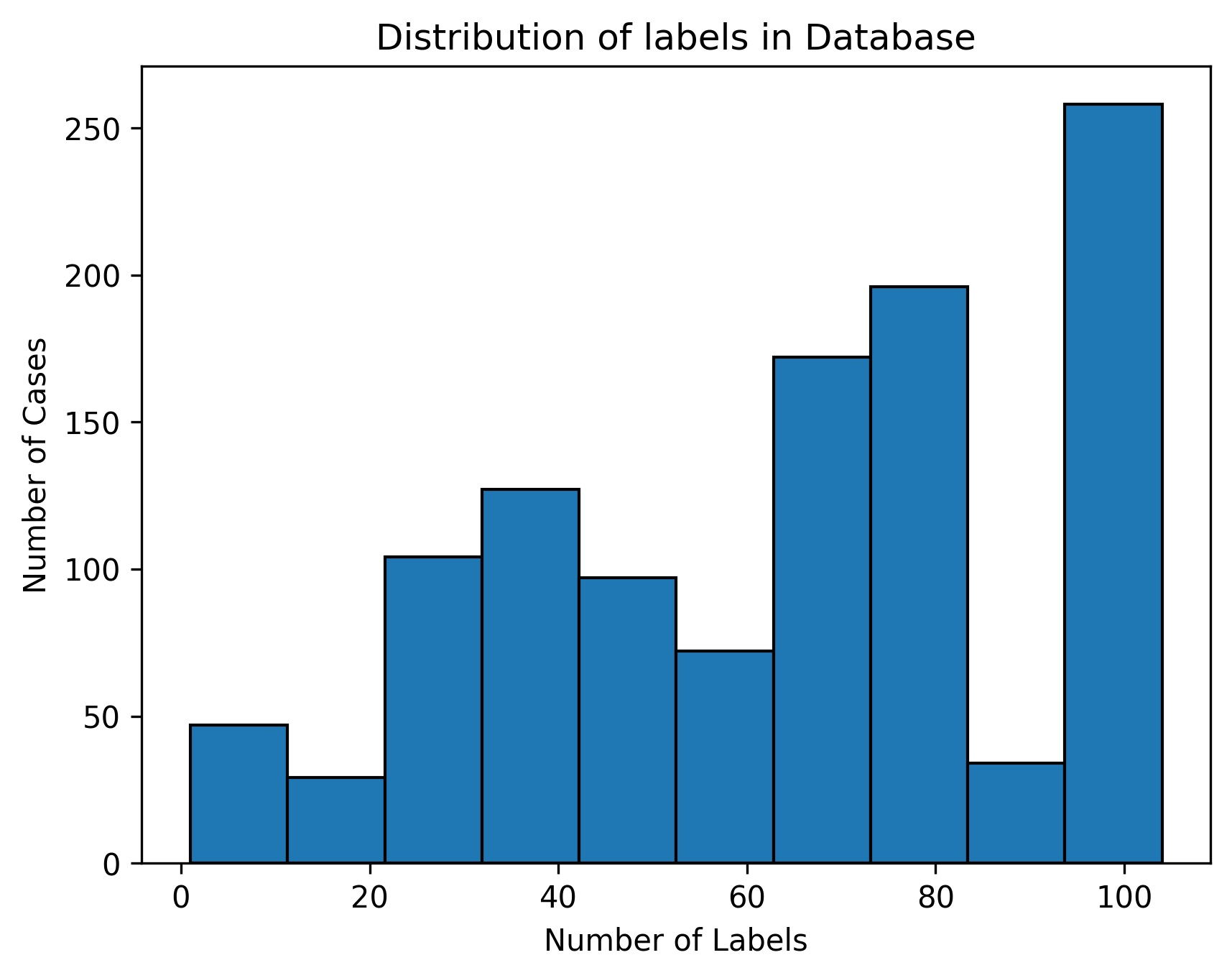
(a)

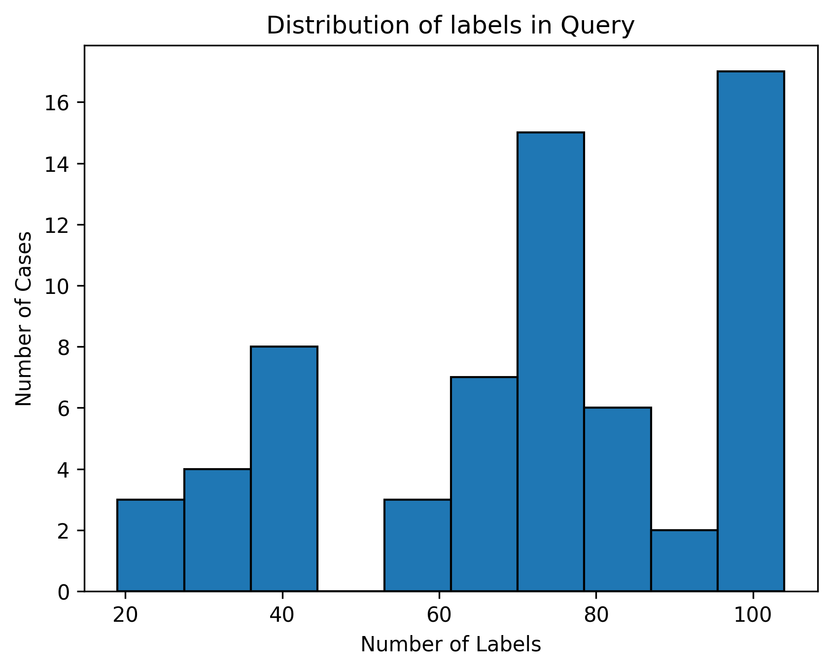
(b)

Figure 4: Distribution of the classes in database (a) and query (b) volumes.

Additionally, it is worth noting that the size and shape of organs can impact the probability of correctly predicting a given label by chance. For example, smaller organs can be less likely to collect "by-chance" true positive predictions compared to larger organs. Similarly, organs with elongated shapes aligned with the slice-wise sampling direction can increase the likelihood of "by-chance" hits. A volume and shape-adjusted representation of recall values does not seem reasonable and thus has not been performed in this work. However, organ volume as shown in Figure 5 and Figure 6 should be considered while interpreting result tables.

Figure 8 and Figure 8 present an overview of mean recall for each of the retrieval methods (all models) versus the mean anatomical region size for 29 and 104 classes, respectively. There is no pattern suggesting any correlation between the size of the anatomical region and the average retrieval recall.

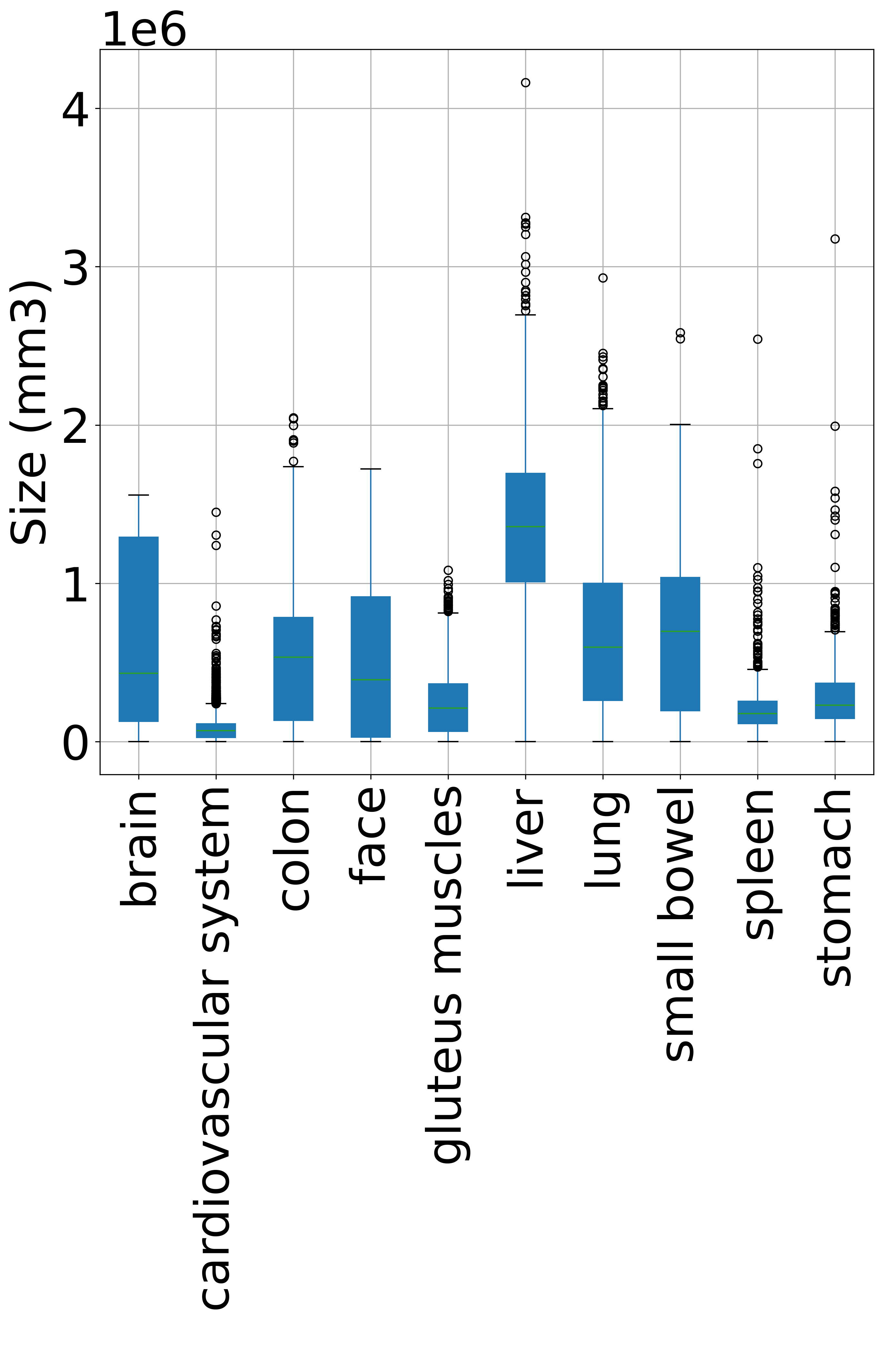
(a)

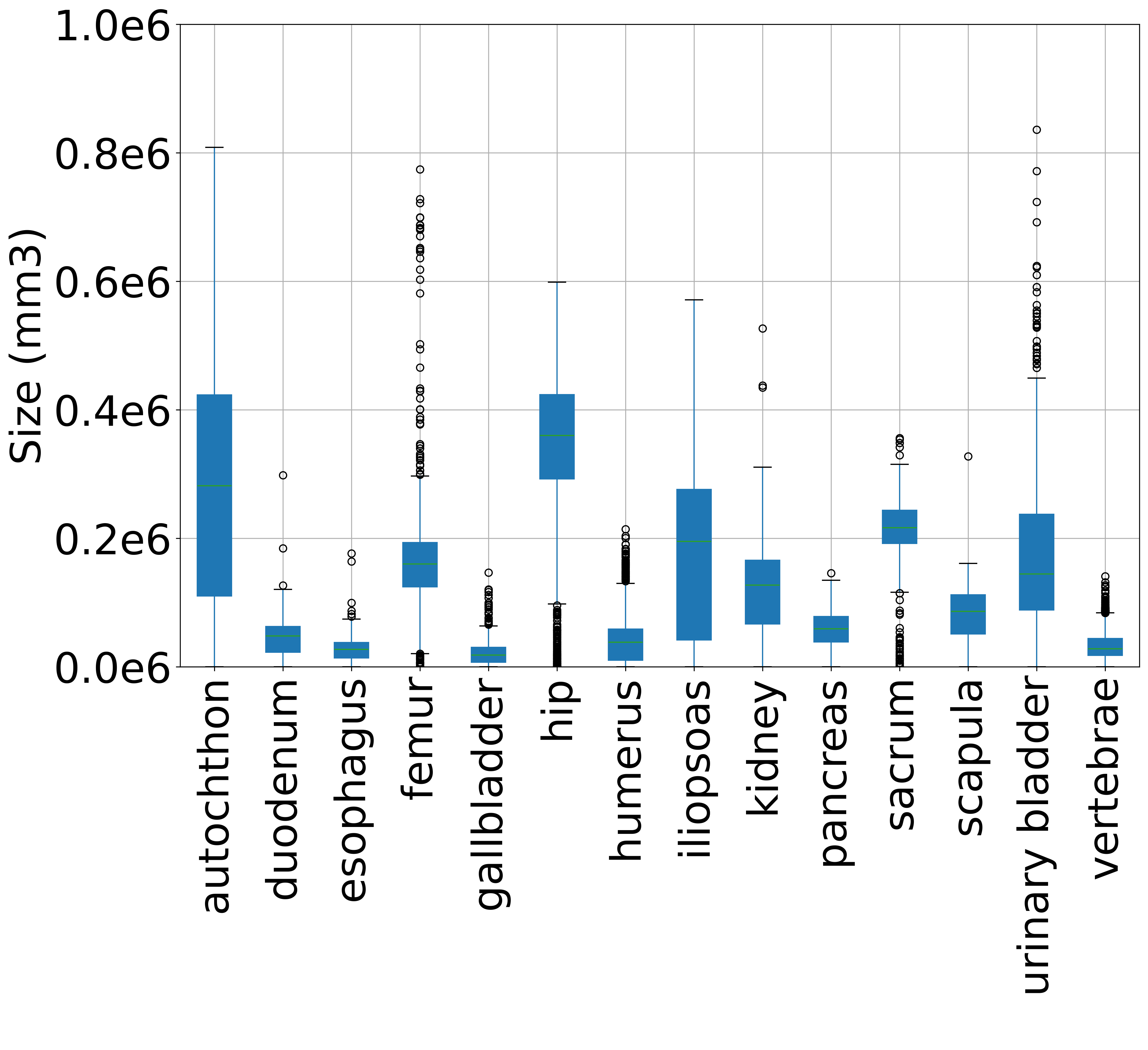
(b)

(c)

Figure 5: distribution of the size of the anatomical regions for the 29 regions (a) big anatomical regions with a physical size range that exceeds $10^{6}$ $mm^{3}$, (b) mid-size anatomical regions with a physical size in range in the range $(.1:1)\times 10^{6}$ $mm^{3}$ and (c) small anatomical regions with a physical size smaller than $.1\times 10^{6}$ $mm^{3}$.

(a)

(b)

(c)

Figure 6: distribution of the size of the anatomical regions for the 104 regions (a) big anatomical regions with a physical size range that exceeds $10^{6}$ $mm^{3}$, (b) mid-size anatomical regions with a physical size in range in the range $(.1:1)\times 10^{6}$ $mm^{3}$ and (c) small anatomical regions with a physical size smaller than $.1\times 10^{6}$ $mm^{3}$.

(a)

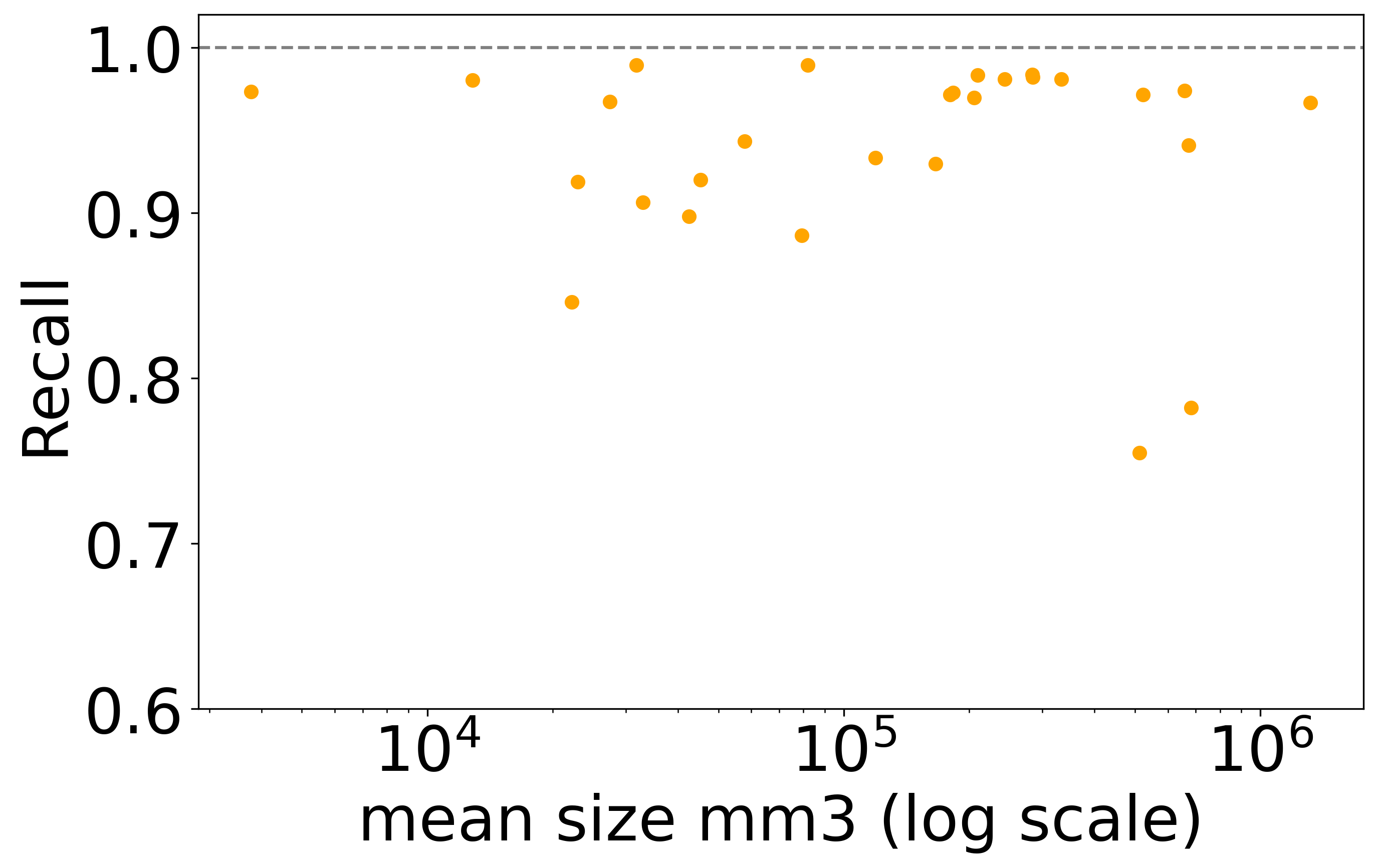
(b)

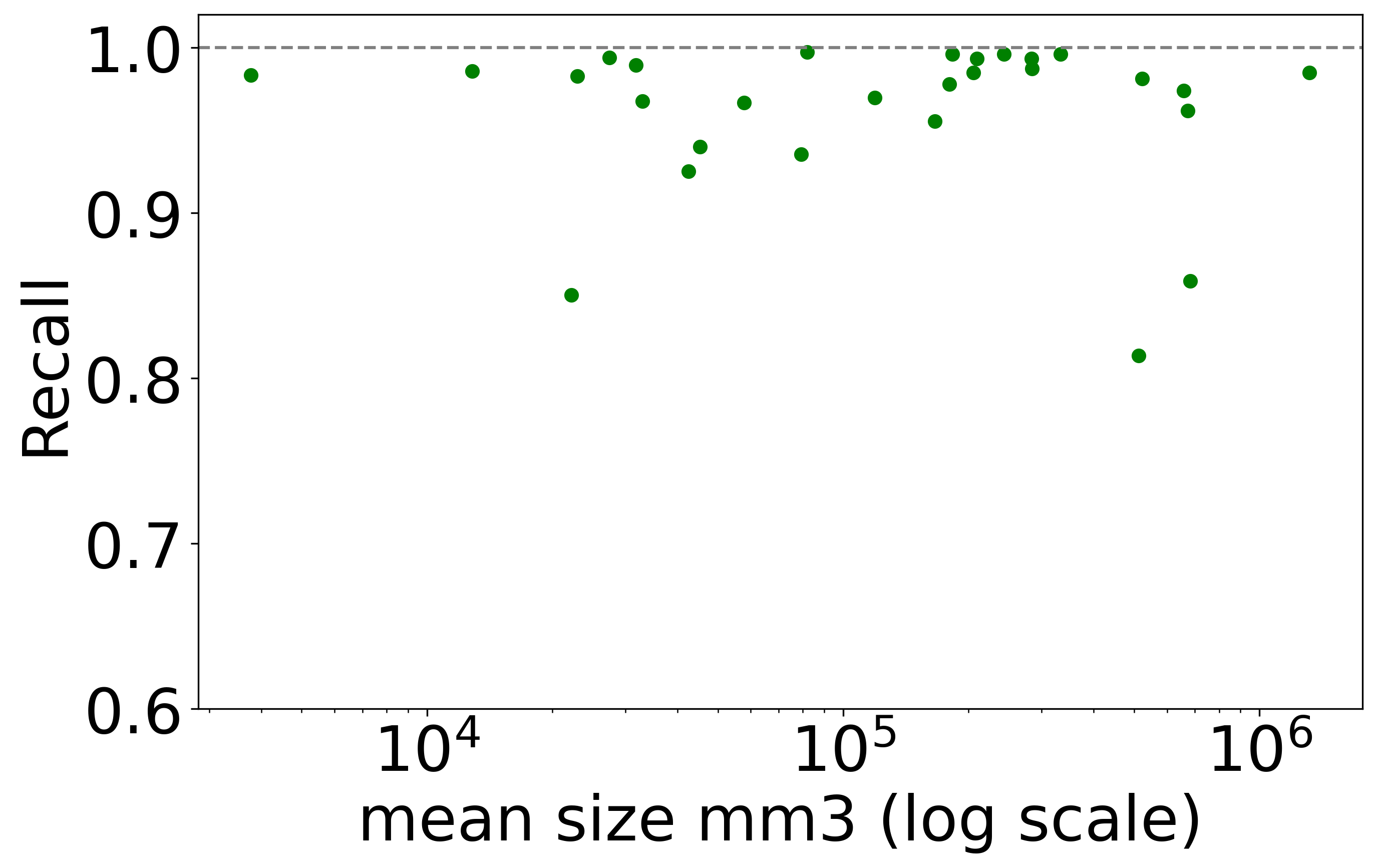
(c)

(d)

(e)

Figure 7: Overview of average recall vs. mean anatomical region size for 29 anatomical regions for (a) slice-wise, (b) volume-based, (c) volume-based and re-ranking, (d) region-based, (e) region-based and re-ranking retrieval.

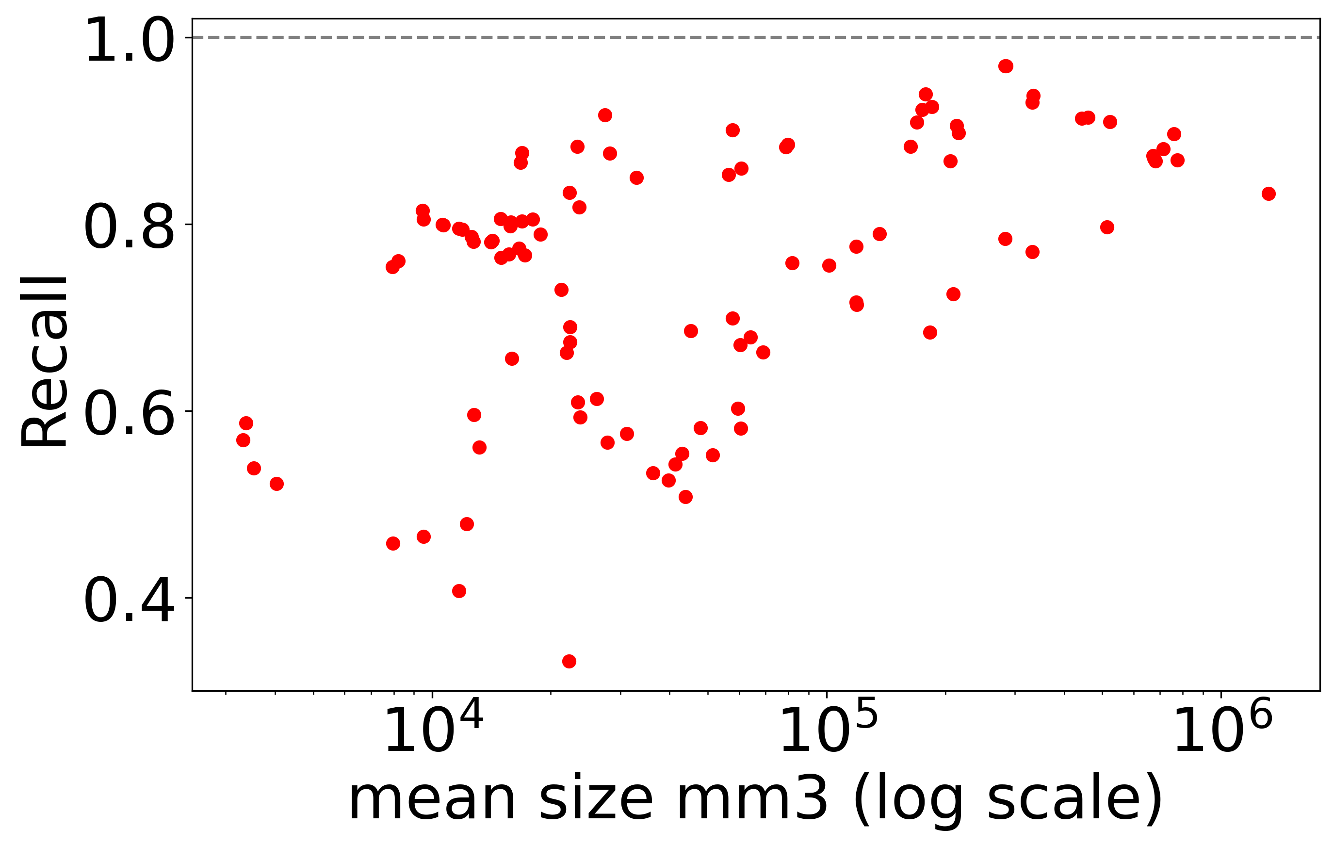
(f)

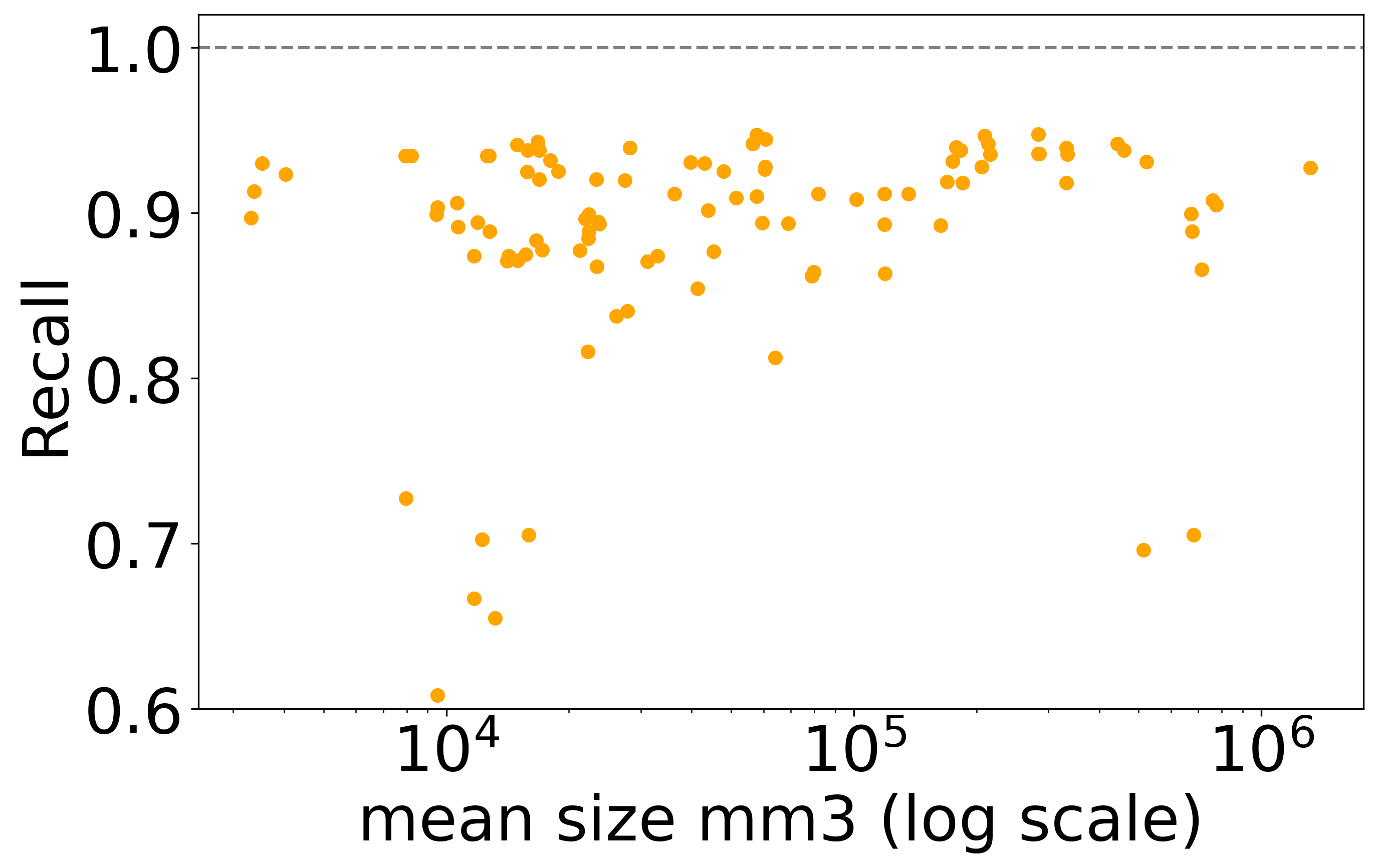
(g)

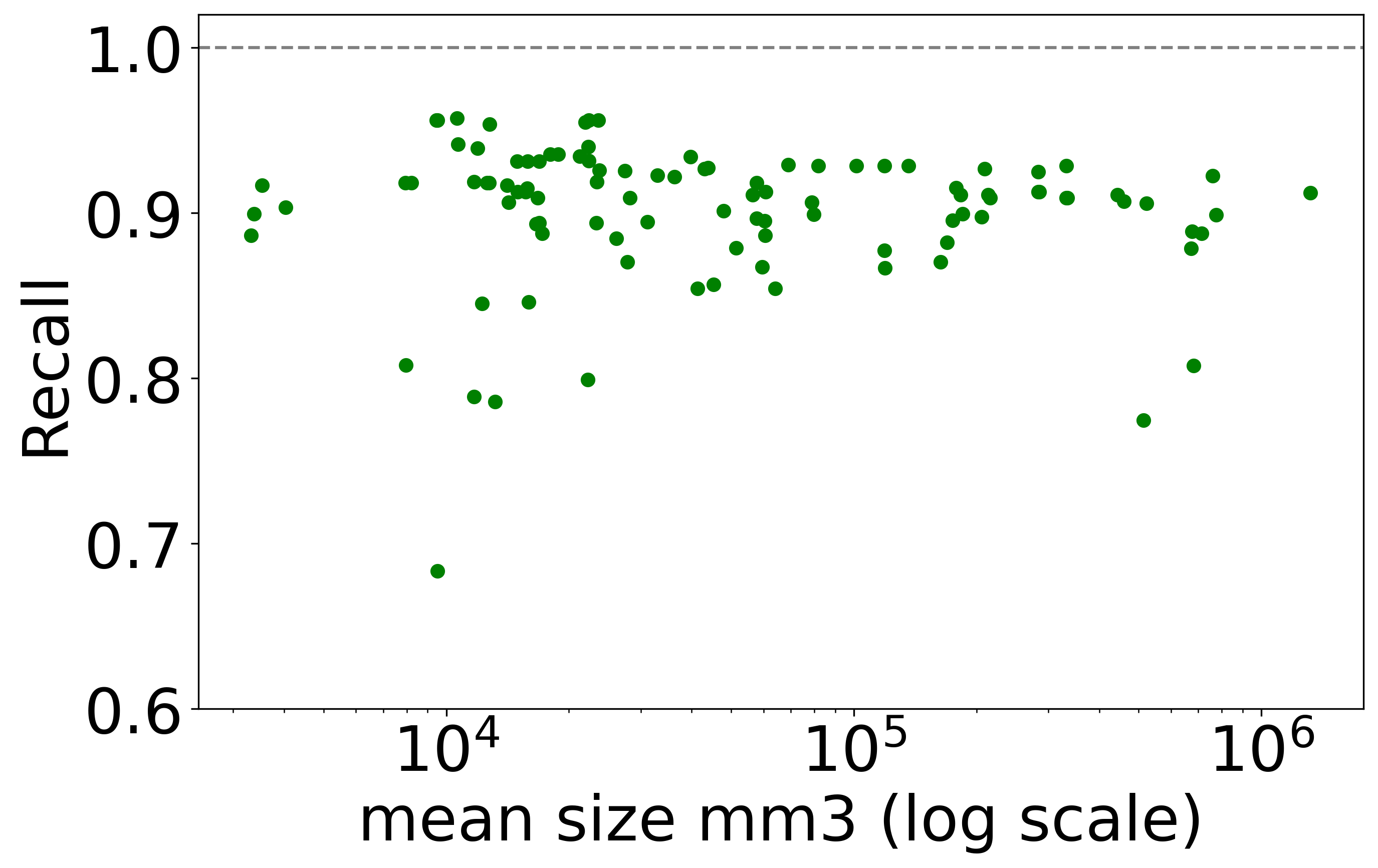
(h)

(i)

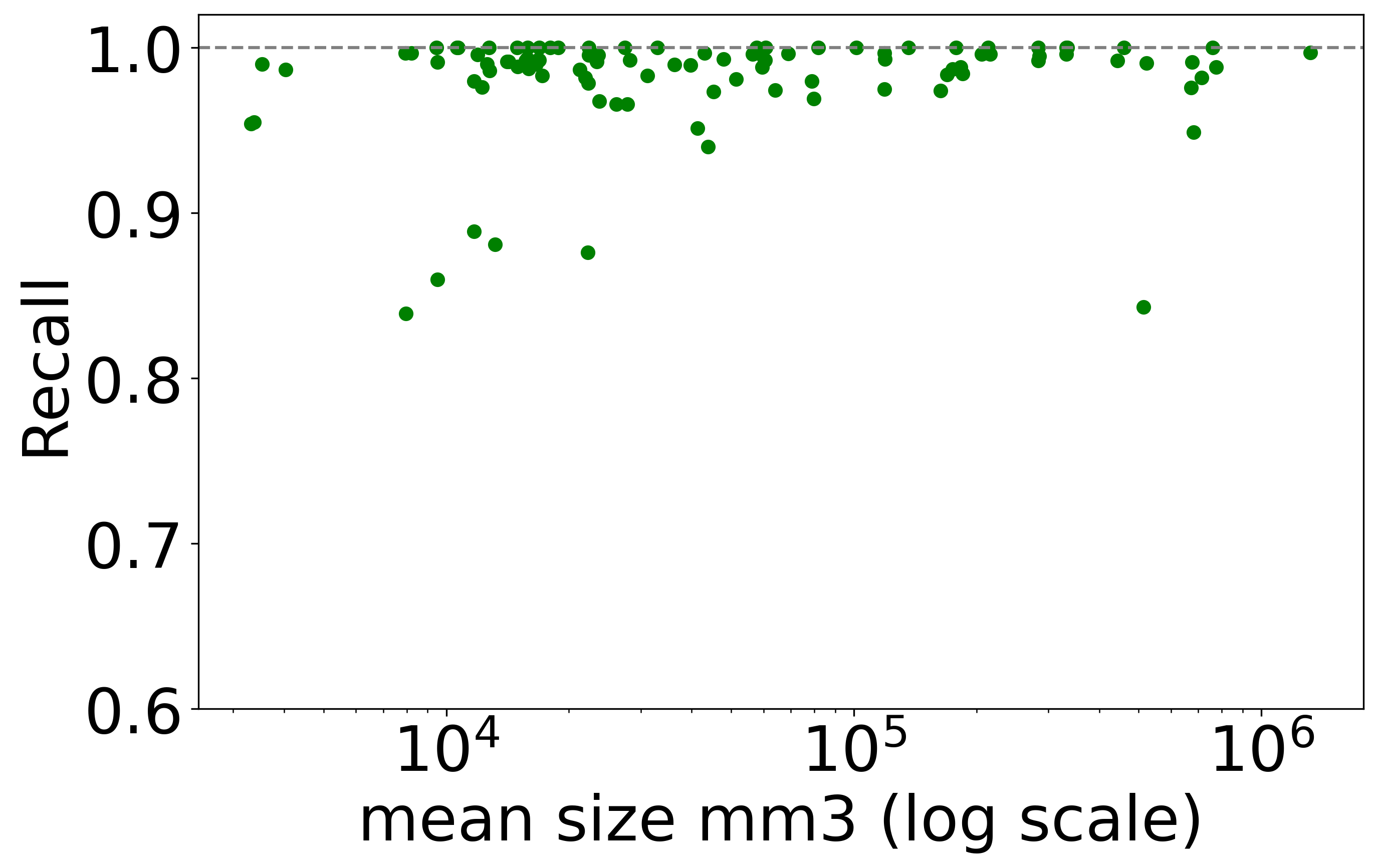
(j)

Figure 8: Overview of average recall vs. mean anatomical region size for 104 anatomical regions for (a) slice-wise, (b) volume-based, (c) volume-based and re-ranking, (d) region-based, (e) region-based and re-ranking retrieval.

4.2 Re-ranking

For the first time, we could successfully show the feasibility of ColBERT-inspired re-ranking out of an image retrieval task. In theory, this shows that CBIR results can be made subject to context-aware re-ranking. This is very important as this provides a conceptual entry point to use the information of a future retrieval solution in the real world. Concretely, observations such as user behavior on a graphical user interface, and temporal or medical relevance can be "factored in" to adjust the search results. Further research will study the advantages and disadvantages of ColBERT-inspired re-ranking. Further insights into balancing computational costs in the context of latency-accuracy trade-offs will be shared.

4.3 Embeddings

It was shown that embeddings generated from self-supervised models are slightly better for image retrieval tasks than those derived from regular supervised models. This is true for coarse anatomical regions with 29 labels (see LABEL:tab:recall-29-regions) as well as fine-granular anatomical regions with 104 regions (see LABEL:tab:recall-104-regions). This is roughly preserved for all modes of retrieval (i.e. slice-wise, volume-based, and region-based). More generally, the differences in recall across differently pre-trained models (except pre-trained from fractal image) are very small and except for slice-wise close to $1.0$. Practically, the exact choice of the feature extractor should not be noticeable to a potential user in a downstream application. Further, it can be concluded that pre-training on general natural images (i.e. ImageNet) resulted in slightly more performant embedding vectors than domain-specific natural images (i.e. RadImageNet). This is somewhat surprising and is subject to further research.

Although, the model pre-trained of formula-derived synthetic images of fractals (i.e. Fractaldb) showed the lowest recall accuracy the absolute values are surprisingly high considering that the model learned visual primitives out of rendered fractals. This is very encouraging as the Formular-Driven Supervised Learning (FDSL) can easily be extended to the very high number of data points per class and also several virtual classes within one family of formulas (Kataoka et al., 2022). Additionally, the mathematical space of formulas for producing visual primitives is virtually infinite and thus it is the subject of further research whether radiology-specific visual primitives can be created that outperform natural image-based pre-training. Again, FDSL does not require the effort of data collection, curation, and annotation. It can scale to a large number of samples and classes which potentially results in a very smooth and evenly covered latent space.

Embeddings derived from DreamSim architecture showed the highest overall retrieval recall in the region-based retrieval with re-ranking. This was true for 29 coarse anatomical regions as well as the original 104 fine-granular regions as used in TotalSegmentator. DreamSim is an ensemble architecture that uses multiple ViT embeddings with additional fine-tuning using synthetic images. It is plausible that an ensemble approach outperforms single-architecture embeddings (i.e. DINOv1, DINOv2, SwinTransformer, and ResNet50). Therefore, the usage of DreamSim is the currently preferred method of embedding generation.

Worth discussing is an observation that can be found in all tables presenting recall values. Across all model architectures (column) there are usually a few anatomies or regions (i.e. row) that show lower recall on average (see "Average" column). For example, in LABEL:tab:slicewise-recall-28-regions "gallbladder" showed poor retrieval accuracy, whereas in Table LABEL:tab:volumewise-recall-29-regions "brain" and "face" showed lower recall. The observation of isolated low-recall patterns can be seen across all modes of retrieval and aggregation. The authors of this paper cannot provide an explanation, as to why certain anatomies perform worse in certain retrieval configurations but gain high recall in many other retrieval configurations. This will be subject to future research.

Table 12: Summary of the average retrieval recall and standard deviation between classes for 29 anatomical regions, the boldfaced values highlight the highest recall across feature extractors.

Model	DINOv1	DINOv2	DreamSim	SwinTrans.	ResNet50
Dataset (pre-trained)	(ImgNet)	(ImgNet)	(ImgNet)	(RadImg)	(Fractaldb)	(RadImg)
slice-wise	$.839\pm.156$	$.819\pm.148$	$\mathbf{.849\pm.148}$	$.824\pm.146$	$.740\pm.167$	$.802\pm.14$
volume-based	$.949\pm.072$	$.932\pm.064$	$.936\pm.063$	$.932\pm.067$	$.939\pm.078$	$\mathbf{.952\pm.04}$
volume-based re-ranked	$\mathbf{.967\pm.040}$	$.961\pm.045$	$.967\pm.045$	$.961\pm.049$	$.962\pm.086$	$.960\pm.050$
region-based	$.977\pm.047$	$.976\pm.051$	$\mathbf{.979\pm.037}$	$.973\pm.042$	$.976\pm.033$	$.978\pm.033$
region-based re-ranked	$.979\pm.045$	$.977\pm.050$	$\mathbf{.987\pm.027}$	$.977\pm.041$	$.981\pm.031$	$.979\pm.04$

Table 13: Summary of the average retrieval recall and standard deviation between classes for 104 anatomical regions, the boldfaced values highlight the highest recall across feature extractors.

Model	DINOv1	DINOv2	DreamSim	SwinTrans.	ResNet50
Dataset (pre-trained)	(ImgNet)	(ImgNet)	(ImgNet)	(RadImg)	(Fractaldb)	(RadImg)
slice-wise	$.784\pm.137$	$.750\pm.144$	$\mathbf{.797\pm.129}$	$.765\pm.140$	$.659\pm.172$	$.726\pm.154$
volume-based	$\mathbf{.923\pm.077}$	$.887\pm.071$	$.892\pm.080$	$.873\pm.082$	$.856\pm.054$	$.908\pm.081$
volume-based re-ranked	$.914\pm.040$	$.880\pm.041$	$.887\pm.040$	$\mathbf{.924\pm.072}$	$.901\pm.061$	$.902\pm.055$
region-based	$.979\pm.037$	$.972\pm.050$	$\mathbf{.983\pm.032}$	$.978\pm.032$	$.973\pm.046$	$.974\pm.042$
region-based re-ranked	$.980\pm.036$	$.978\pm.042$	$\mathbf{.987\pm.024}$	$.981\pm.033$	$.982\pm.042$	$.980\pm.041$

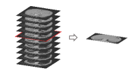
(a)

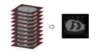
(b)

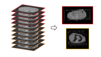
(c)

Figure 9: An overview of three retrieval methods: (a) Slice-wise, where the retrieval is based on one selected slice e.g., the user zooms to a slice and retrieves the most similar slice (b) volume-based, where the retrieval is based on a complete volume, e.g., the user would like to retrieve similar volumes to the volumes under examination or simply filter the database (c) region-based, where the retrieval is based on the selected organ (or sub-volume), e.g, the user zooms in to a specific region and the most similar volume containing that region is retrieved.

4.4 Volume-based vs Region-based Retrieval

Since multiple organs (i.e. labels) are present in each query volume, there are essentially two ways in which image retrieval can be performed. The preferred choice depends on the context of the retrieval task in the real world. If the goal is to find a scan out of a database that is most similar to a complete query scan with the entirety of all present organs (think scan-id to scan-id but visual), then volume-based retrieval is the right choice. In contrast, if the experimenter is interested in a particular organ and its most similar counterpart in the database (and all other organs just happen to be in the same scan due to proximity), then region-based retrieval is advised. The second query scenario offers a higher retrieval recall. The slice-wise retrieval can find the most similar slice of a volume regardless of other slices. This is not usually a practical choice in real scenarios. Figure 9 visualizes the options.

5 Conclusion

Our study establishes a new benchmark for the retrieval of anatomical structures within 3D medical volumes, utilizing the TotalSegmentator dataset to facilitate targeted queries of volumes or sub-volumes for specific anatomical structures. The results highlight the potential of leveraging pre-trained embeddings, originally trained on non-medical images, for medical image retrieval across diverse anatomical regions with a wide size range.

We introduced a re-ranking method based on a late interaction model from text retrieval, i.e. ColBERT Khattab and Zaharia (2020). The proposed ColBERT-inspired method enhances the retrieval recall of all anatomical regions. Future investigations can focus on refining and optimizing the computational efficiency of the proposed re-ranking method.

We evaluated the performance of different embeddings pre-trained supervised and self-supervised on medical and non-medical data. The results indicate that pre-training on general natural images (e.g., ImageNet) yields slightly more effective embedding vectors than domain-specific natural images (e.g., RadImageNet). However, given the marginal difference, the choice of embeddings is unlikely to impact the user experience in downstream tasks significantly.

The retrieval of certain anatomical structures, such as the brain and face, demonstrates low recall across all embedding and retrieval methods. Subsequent research can explore the prevalence of such patterns and potential solutions.

This benchmark sets the stage for future advancements in content-based medical image retrieval, particularly in localizing specific organs or areas within scans.

References

- Dubey [2021] Shiv Ram Dubey. A decade survey of content based image retrieval using deep learning. IEEE Transactions on Circuits and Systems for Video Technology, 32(5):2687–2704, 2021.
- Khun Jush et al. [2023] Farnaz Khun Jush, Tuan Truong, Steffen Vogler, and Matthias Lenga. Medical image retrieval using pretrained embeddings. arXiv preprint arXiv:2311.13547, 2023.
- Wang et al. [2022] Wenqing Wang, Pengfei Jiao, Han Liu, Xiao Ma, and Zhuo Shang. Two-stage content based image retrieval using sparse representation and feature fusion. Multimedia Tools and Applications, 81(12):16621–16644, 2022.
- Qayyum et al. [2017] Adnan Qayyum, Syed Muhammad Anwar, Muhammad Awais, and Muhammad Majid. Medical image retrieval using deep convolutional neural network. Neurocomputing, 266:8–20, 2017.
- Abacha et al. [2023] Asma Ben Abacha, Alberto Santamaria-Pang, Ho Hin Lee, Jameson Merkow, Qin Cai, Surya Teja Devarakonda, Abdullah Islam, Julia Gong, Matthew P Lungren, Thomas Lin, et al. 3d-mir: A benchmark and empirical study on 3d medical image retrieval in radiology. arXiv preprint arXiv:2311.13752, 2023.
- Denner et al. [2024] Stefan Denner, David Zimmerer, Dimitrios Bounias, Markus Bujotzek, Shuhan Xiao, Lisa Kausch, Philipp Schader, Tobias Penzkofer, Paul F Jäger, and Klaus Maier-Hein. Leveraging foundation models for content-based medical image retrieval in radiology. arXiv preprint arXiv:2403.06567, 2024.
- Truong et al. [2023] Tuan Truong, Farnaz Khun Jush, and Matthias Lenga. Benchmarking pretrained vision embeddings for near-and duplicate detection in medical images. arXiv preprint arXiv:2312.07273, 2023.
- Antonelli et al. [2022] Michela Antonelli, Annika Reinke, Spyridon Bakas, Keyvan Farahani, Annette Kopp-Schneider, Bennett A Landman, Geert Litjens, Bjoern Menze, Olaf Ronneberger, Ronald M Summers, et al. The medical segmentation decathlon. Nature communications, 13(1):4128, 2022.
- Wasserthal et al. [2023] Jakob Wasserthal, Hanns-Christian Breit, Manfred T Meyer, Maurice Pradella, Daniel Hinck, Alexander W Sauter, Tobias Heye, Daniel T Boll, Joshy Cyriac, Shan Yang, et al. Totalsegmentator: Robust segmentation of 104 anatomic structures in ct images. Radiology: Artificial Intelligence, 5(5), 2023.
- Khattab and Zaharia [2020] Omar Khattab and Matei Zaharia. Colbert: Efficient and effective passage search via contextualized late interaction over bert. In Proceedings of the 43rd International ACM SIGIR conference on research and development in Information Retrieval, pages 39–48, 2020.
- Aumüller et al. [2020] Martin Aumüller, Erik Bernhardsson, and Alexander Faithfull. Ann-benchmarks: A benchmarking tool for approximate nearest neighbor algorithms. Information Systems, 87:101374, 2020.
- Malkov and Yashunin [2018] Yu A Malkov and Dmitry A Yashunin. Efficient and robust approximate nearest neighbor search using hierarchical navigable small world graphs. IEEE transactions on pattern analysis and machine intelligence, 42(4):824–836, 2018.
- Taha et al. [2024] Ibraheem Taha, Matteo Lissandrini, Alkis Simitsis, and Yannis Ioannidis. A study on efficient indexing for table search in data lakes. In 2024 IEEE 18th International Conference on Semantic Computing (ICSC), pages 245–252. IEEE, 2024.
- Johnson et al. [2019] Jeff Johnson, Matthijs Douze, and Hervé Jégou. Billion-scale similarity search with gpus. IEEE Transactions on Big Data, 7(3):535–547, 2019.
- Deng et al. [2009] Jia Deng, Wei Dong, Richard Socher, Li-Jia Li, Kai Li, and Li Fei-Fei. Imagenet: A large-scale hierarchical image database. In 2009 IEEE conference on computer vision and pattern recognition, pages 248–255. Ieee, 2009.
- Caron et al. [2021] Mathilde Caron, Hugo Touvron, Ishan Misra, Hervé Jégou, Julien Mairal, Piotr Bojanowski, and Armand Joulin. Emerging properties in self-supervised vision transformers. In Proceedings of the IEEE/CVF international conference on computer vision, pages 9650–9660, 2021.
- Oquab et al. [2023] Maxime Oquab, Timothée Darcet, Théo Moutakanni, Huy Vo, Marc Szafraniec, Vasil Khalidov, Pierre Fernandez, Daniel Haziza, Francisco Massa, Alaaeldin El-Nouby, et al. Dinov2: Learning robust visual features without supervision. arXiv preprint arXiv:2304.07193, 2023.
- Fu et al. [2023] Stephanie Fu, Netanel Tamir, Shobhita Sundaram, Lucy Chai, Richard Zhang, Tali Dekel, and Phillip Isola. Dreamsim: Learning new dimensions of human visual similarity using synthetic data. arXiv preprint arXiv:2306.09344, 2023.
- Liu et al. [2021] Ze Liu, Yutong Lin, Yue Cao, Han Hu, Yixuan Wei, Zheng Zhang, Stephen Lin, and Baining Guo. Swin transformer: Hierarchical vision transformer using shifted windows. In Proceedings of the IEEE/CVF international conference on computer vision, pages 10012–10022, 2021.
- He et al. [2016] Kaiming He, Xiangyu Zhang, Shaoqing Ren, and Jian Sun. Deep residual learning for image recognition. In Proceedings of the IEEE conference on computer vision and pattern recognition, pages 770–778, 2016.
- Mei et al. [2022] Xueyan Mei, Zelong Liu, Philip M Robson, Brett Marinelli, Mingqian Huang, Amish Doshi, Adam Jacobi, Chendi Cao, Katherine E Link, Thomas Yang, et al. Radimagenet: an open radiologic deep learning research dataset for effective transfer learning. Radiology: Artificial Intelligence, 4(5):e210315, 2022.
- Kataoka et al. [2022] Hirokatsu Kataoka, Kazushige Okayasu, Asato Matsumoto, Eisuke Yamagata, Ryosuke Yamada, Nakamasa Inoue, Akio Nakamura, and Yutaka Satoh. Pre-training without natural images. International Journal of Computer Vision (IJCV), 2022.
- Ai et al. [2018] Qingyao Ai, Jiaxin Mao, Yiqun Liu, and W Bruce Croft. Unbiased learning to rank: Theory and practice. In Proceedings of the 27th ACM International Conference on Information and Knowledge Management, pages 2305–2306, 2018.
- Guo et al. [2020] Jiafeng Guo, Yixing Fan, Liang Pang, Liu Yang, Qingyao Ai, Hamed Zamani, Chen Wu, W Bruce Croft, and Xueqi Cheng. A deep look into neural ranking models for information retrieval. Information Processing & Management, 57(6):102067, 2020.
- MacAvaney et al. [2019] Sean MacAvaney, Andrew Yates, Arman Cohan, and Nazli Goharian. Cedr: Contextualized embeddings for document ranking. In Proceedings of the 42nd international ACM SIGIR conference on research and development in information retrieval, pages 1101–1104, 2019.
- Devlin et al. [2018] Jacob Devlin, Ming-Wei Chang, Kenton Lee, and Kristina Toutanova. Bert: Pre-training of deep bidirectional transformers for language understanding. arXiv preprint arXiv:1810.04805, 2018.
- Santhanam et al. [2021] Keshav Santhanam, Omar Khattab, Jon Saad-Falcon, Christopher Potts, and Matei Zaharia. Colbertv2: Effective and efficient retrieval via lightweight late interaction. arXiv preprint arXiv:2112.01488, 2021.