Leveraging graphical model techniques to study evolution on phylogenetic networks

Abstract

The evolution of molecular and phenotypic traits is commonly modelled using Markov processes along a rooted phylogeny. This phylogeny can be a tree, or a network if it includes reticulations, representing events such as hybridization or admixture. Computing the likelihood of data observed at the leaves is costly as the size and complexity of the phylogeny grows. Efficient algorithms exist for trees, but cannot be applied to networks. We show that a vast array of models for trait evolution along phylogenetic networks can be reformulated as graphical models, for which efficient belief propagation algorithms exist. We provide a brief review of belief propagation on general graphical models, then focus on linear Gaussian models for continuous traits. We show how belief propagation techniques can be applied for exact or approximate (but more scalable) likelihood and gradient calculations, and prove novel results for efficient parameter inference of some models. We highlight the possible fruitful interactions between graphical models and phylogenetic methods. For example, approximate likelihood approaches have the potential to greatly reduce computational costs for phylogenies with reticulations.

Keywords belief propagation, cluster graph, admixture graph, trait evolution, Brownian motion, linear Gaussian

1 Introduction

In phylogenetics, data are observed at the leaves of a phylogeny: a directed acyclic graph representing the historical relationships between species, populations or individuals of interest, with branch lengths representing evolutionary time and internal nodes representing divergence (e.g. speciation) or merging (e.g. introgression) events. Stochastic processes are used to model the evolution of traits over time along this phylogeny. In this work, we consider traits that may be multivariate, discrete and/or continuous, with a focus on continuous traits. Inference from these models are used to infer evolutionary dynamics and historical correlation between traits, predict unobserved traits at ancestral nodes or extant leaves, or estimate phylogenies from rich data sets.

Calculating the likelihood is no easy task because the traits at ancestral nodes are unobserved and need to be integrated out. This problem is very well studied for phylogenetic trees, with efficient solutions for both discrete and continuous traits. Admixture graphs and phylogenetic networks with reticulations are now gaining traction due to growing empirical evidence for gene flow, hybridization and admixture. Yet many methods and tools for these networks could be improved towards more efficient likelihood calculations.

The vast majority of evolutionary models used in phylogenetics make a Markov assumption, in that the trait distribution at all nodes (observed at the tips and unobserved at internal nodes) can be expressed by a set of local models. At the root, this model describes the prior distribution of the ancestral trait. For each node in the phylogeny, a local transition model describes the trait distribution at this node conditional on the trait(s) at its parent node(s). As each local model can be specified individually with its own set of parameters, the overall evolutionary model can be very flexible, including possible shifts in rates, constraints, and mode of evolution across different clades. Other models do not make a Markov assumption, such as models that combine a backwards-in-time coalescent process for gene trees and forward-in-time mutation process along gene trees. We show here that some of these models can still be expressed as a product of local conditional distributions, over a graph that is more complex than the initial phylogeny.

These evolutionary models are special cases of graphical models, also known as Bayesian networks, which have been heavily studied. The task of calculating the likelihood of the observed data has received a lot of attention, including algorithms for efficient approximations when the network is too complex to calculate the likelihood exactly. Another well-studied task is that of predicting the state of unobserved variables (ancestral states in phylogenetics) conditional on the observed data. We argue here that the field of phylogenetics could greatly benefit from applying and expanding knowledge from graphical models for the study and use of phylogenetic networks.

In section 2 we review the challenge brought by phylogenetic models in which only tip data are observed, and the techniques currently used for efficient likelihood calculations for phylogenetic models on trees and networks. In section 3 we focus on the general Gaussian models for the evolution of a continuous trait, possibly multivariate to capture evolutionary correlations between traits. On reticulate phylogenies, these models need to describe the trait of admixed populations conditional on their parental populations. Turning to graphical models in section 4, we describe their general formulation and show that many phylogenetic models can be expressed as special cases, from known examples (on gene trees) to less obvious examples (using the coalescent process on species trees, or species networks). We then provide a short review of belief propagation, a core technique to perform inference on graphical models, first in its general form and then specialized for continuous traits in linear Gaussian models. In section 5 we describe loopy belief propagation, a technique to perform approximation inference in graphical models, when exact inference does not scale. As far as we know, loopy belief propagation has never been used in phylogenetics. Section 6 describes leveraging BP for parameter inference: fast calculations of the likelihood and its gradient can be used in any likelihood-based framework, frequentist or Bayesian. Finally, section 7 discusses future challenges for the application and extension of graphical model techniques in phylogenetics. These techniques offer a range of avenues to expand the phylogeneticists’ toolbox for fitting evolutionary models on phylogenetic networks, from approximate inference methods that are more scalable, to algorithms for fast gradient computation for better parameter inference.

2 Complexity of the phylogenetic likelihood calculation

2.1 The pruning algorithm

Felsenstein’s pruning algorithm Felsenstein [1973, 1981] launched the era of model-based phylogenetic inference, now rich with complex models to account for a large array of biological processes: including DNA and protein substitution models, variation of their substitution rates across genomic loci, lineages and time, and evolutionary models for continuous traits and geographic distributions. The pruning algorithm gave the key to calculate the likelihood of these models along a phylogenetic tree, in a practically feasible way. The basis of this algorithm, which extends to tasks beyond likelihood calculation, was discovered in other areas and given other names, such as the sum-product algorithm, message passing, and belief propagation (BP).

The pruning algorithm, which is a form of BP, computes the the full likelihood of all the observed taxa by traversing the phylogenetic tree once, taking advantage of the Markov property: where the evolution of the trait of interest along a daughter lineage is independent of its past evolution, given knowledge of the parent’s state. The idea is to traverse the tree and calculate the likelihood of the descendant leaves of an ancestral species conditional on its state, from similar likelihoods calculated for each of its children. If the trait is discrete with 4 states for example (as for DNA), then this entails keeping track of 4 likelihood values at each ancestral species. If the trait is continuous with a Gaussian distribution, e.g. from a Brownian motion (BM) or an Ornstein-Uhlenbeck (OU) process Hansen [1997], then the likelihood at an ancestral species is a nice function of its state that can be concisely parametrized by quantities akin to the posterior mean and variance conditional on descendant leaves. Felsenstein’s independent contrasts (IC) Felsenstein [1985] also captures these partial posterior quantities and can be viewed as a special implementation of BP for likelihood calculation.

BP is used ubiquitously for the analysis of discrete traits, such as for DNA substitution models (e.g. in RAxML Stamatakis [2014], IQ-TREE Nguyen et al. [2015], MrBayes Ronquist and Huelsenbeck [2003]) or for discrete morphological traits in comparative methods (e.g. in phytools Revell [2012], BayesTraits Pagel et al. [2004], corHMM Boyko and Beaulieu [2021], Boyko et al. [2023], RevBayes Höhna et al. [2016]). For discrete traits, there is simply no feasible alternative. On a tree with 20 taxa and 19 ancestral species, the naive calculation of the likelihood at a given DNA site would require the calculation and summation of $4^{19}$ or 274 billion likelihoods, one for each nucleotide assignment at the 19 ancestral species. This calculation would need to be repeated for each site in the alignment, then repeated all over during the search for a well-fitting phylogenetic tree.

2.2 Continuous traits on trees: the lazy way

For continuous traits under a Gaussian model (including the Brownian motion), BP is not used as ubiquitously because a multivariate Gaussian distribution can be nicely captured by its mean and covariance matrix: the multivariate Gaussian formula can serve as an alternative. For example, for one trait $Y$ with ancestral state $\mu$ at the root of the phylogeny, the phylogenetic covariance $\bm{\Sigma}$ between the taxa at the leaves can be obtained from the branch lengths in the tree. Under a BM, the covariance $\operatorname{cov}(Y_{i},Y_{j})$ between taxa $i$ and $j$ is $\Sigma_{ij}=\sigma^{2}t_{ij}$ where $t_{ij}$ is the length between the root and their most recent common ancestor. The likelihood of the observed traits at the $n$ leaves can then be calculated using matrix and vector multiplication techniques as

$$(2\pi)^{-n/2}\det|\bm{\Sigma}|^{-1/2}\exp\left(-\frac{1}{2}(Y-\mu)^{\top}\bm{\Sigma}^{-1}(Y-\mu)\right).$$ (1)

This alternative to BP has the disadvantage of requiring the inversion of the covariance matrix $\bm{\Sigma}$, a task whose computing time typically grows as $m^{3}$ for a matrix of size $m\times m$. It also has the disadvantage that $\bm{\Sigma}$ needs to be calculated and stored in memory in the first place. For multivariate observations of $p$ traits on each of $n$ taxa, the covariance matrix has size $m=pn$ so the typical calculation cost of (1) is then $O(p^{3}n^{3})$, which can quickly become very large. For example, with only 30 taxa and 10 traits, $\bm{\Sigma}$ is a $300\times 300$-matrix. Studies with large $p$ and/or large $n$ are now frequent, especially from geometric morphometric data with $p$ over 100 typically (e.g. Hedrick [2023]) or with expression data on $p>1000$ genes easily, that also require more complex models to account for variation (e.g. within species, between organs, between batches) Dunn et al. [2013], Shafer [2019]. Studies with a large number $n$ of taxa are now frequent (e.g. $n>5,000$ in birds and mammals Jetz et al. [2012], Upham et al. [2019]) and virus phylogenies can be massive (e.g. $n>1000$ and $p=3$ virulence traits in HIV Hassler et al. [2022a], or $n>500,000$ SARS-CoV-2 strains De Maio et al. [2023]).

In these cases with large data size $np$, the matrix-based alternative to BP is prone to numerical inaccuracy and numerical instability in addition to the increased computational time, because it is hard to accurately invert a large matrix. Even when the matrix is of moderate size, numerical inaccuracy can arise when the matrix is “ill-conditioned”. These problems were identified under OU models on phylogenetic trees that have closely-related sister taxa, or under early-burst (EB) models with strong morphological diversification early on during the group radiation, and much slowed-down evolution later on Adams and Collyer [2017], Jhwueng and O’Meara [2020], Bartoszek et al. [2023].

For some simple models, the large $np\times np$ covariance matrix can be decomposed as a Kronecker product of a $p\times p$ trait covariance and a $n\times n$ phylogenetic covariance. This decomposition can simplify the complexity of calculating the likelihood. However, this decomposition is not available under many models, such as the multivariate Brownian motion with shifts in the evolutionary rates (e.g. Caetano and Harmon [2019]) or the multivariate Ornstein-Uhlenbeck model with non-scalar rate or selection matrices Bartoszek et al. [2012], Clavel et al. [2015].

2.3 BP for continuous traits on trees

To bypass the complexity of matrix inversion, Felsenstein pioneered IC to test for phylogenetic correlation between traits, assuming a BM model on a tree Felsenstein [1985]. Many authors then used BP approaches to handle Gaussian models beyond the BM FitzJohn [2012], Freckleton [2012], Cybis et al. [2015], Goolsby et al. [2017]. Notably, Ho and Ané [2014] describe a fast algorithm that can be used for non-Gaussian models as well. Most recently, Mitov et al. [2020] highlighted that BP can be applied to a large class of Gaussian models: including the BM and the OU process with shifts and variation of rates and selection regimes across branches. Software packages that use these fast BP algorithms include phylolm Ho and Ané [2014], Rphylopars Goolsby et al. [2017], BEAST Hassler et al. [2023] or the most recent versions of hOUwie Boyko et al. [2023] and mvSLOUCH Bartoszek et al. [2023].

All the methods cited above only use the first post-order tree traversal of BP to compute the likelihood. A second preorder traversal allows, in the Gaussian case, for the computation of the distribution of all internal nodes conditionally on the model and on the traits values at the tips. These distributions can then be used for, e.g., ancestral state reconstruction Lartillot [2014], expectation-maximization algorithms for shift detection in the optimal values of an OU Bastide et al. [2018a], or the computation of the gradient of the likelihood in the BM Zhang et al. [2021], Fisher et al. [2021] or general Gaussian model Bastide et al. [2021]. Such BP techniques have also been used for taking gradients of the likelihood with respect to branch lengths in sequence evolution models Ji et al. [2020] or for phylogenetic factor analysis Tolkoff et al. [2018], Hassler et al. [2022b].

2.4 From trees to networks

So far, Felsenstein’s pruning algorithm and related BP approaches have been restricted to phylogenetic trees, mostly. There is now ample evidence that reticulation is ubiquitous in all domains of life from biological processes such as lateral gene transfer, hybridization, introgression and gene flow between populations. Networks are recognized to be better than trees for representing the phylogenetic history of species and populations in many groups. Although current studies using networks have few taxa, typically between 10-20 (e.g. Nielsen et al. [2023]), they tend to have increasingly more tips as network inference methods become more scalable (e.g. $n=39$ languages in Neureiter et al. [2022]). As viruses are known to be affected by recombination, we also expect future virus studies to use large network phylogenies Ignatieva et al. [2022], so that BP will become essential for network studies too. In this work, we describe approaches currently used for trait evolution on phylogenetic networks. We argue that the field of evolutionary biology would benefit from applying BP approaches on networks more systematically. Transferring knowledge from the mature and rich literature on BP would advance evolutionary biology research when phylogenetic networks are used.

2.5 Current network approaches for discrete traits

For discrete traits on general networks, very few approaches use BP techniques as far as we know. For DNA data for example, PhyLiNC Allen-Savietta [2020] and NetRAX Lutteropp et al. [2022] extend the typical tree-based model to general networks, assuming no incomplete lineage sorting. That is, each site is assumed to evolve along one of the trees displayed in the network, chosen according to inheritance probabilities at reticulate edges. PhyLiNC assumes independent (unlinked) sites. NetRAX assumes independent loci, which may have a single site each. Each locus may have its own set of branch lengths and substitution model parameters. Both methods calculate the likelihood of a network $N$ via extracting its displayed trees and then applying BP on each tree. Similarly, comparative methods for binary and multi-state traits implemented in PhyloNetworks also extract displayed trees and then apply BP on each displayed tree Karimi et al. [2020]. While these approaches use BP on each displayed tree, a network with $h$ reticulations can have up to $2^{h}$ displayed trees. This leads to a computational bottleneck when the number of reticulations increases.

BP approaches have also been used for models with incomplete lineage sorting, modelled by the coalescent Kingman [1982]. Notably, SNAPP models the evolution of unlinked biallelic markers along a species tree, accounting for incomplete lineage sorting Bryant et al. [2012]. This method was recently made faster with SNAPPER Stoltz et al. [2020] and extended to phylogenetic networks with SnappNet Rabier et al. [2021]. The coalescent process introduces the challenge that each site may evolve along any tree, depending on past coalescent events. SNAPP introduced a way to bypass the difficulties of handling coalescent histories and hence decrease computation time. After we describe BP for general graphical models, we recast this innovation as BP on a graphical model formulation of the problem.

BP was also used to calculate the likelihood of the joint sample frequency spectrum (SFS). To account for incomplete lineage sorting on a tree, Kamm et al. [2017] use the continuous-time Moran model to reduce computational complexity, and assume that each site undergoes at most one mutation. In momi2, Kamm et al. [2020] extend the approach to phylogenetic networks by assuming a pulse of admixture at reticulations. The associated graphical model is much simpler than that required by SNAPP or SnappNet thanks to the assumption of no recurrent mutation.

2.6 Current network approaches for continuous traits

Compared to the rich toolkit available for the analysis of continuous traits on trees, the toolkit for phylogenetic networks is still limited. PhyloNetworks includes comparative methods on networks Solís-Lemus et al. [2017], implemented in Julia Bezanson et al. [2017]. These methods extend phylogenetic ANOVA to networks, for a continuous response trait predicted by any number of continuous or categorical traits, with residual variation being phylogenetically correlated. So far, the models available in PhyloNetworks include the BM, Pagel’s $\lambda$, possible within-species variation, and shifts at reticulations to model transgressive evolution Bastide et al. [2018b], Teo et al. [2023]. However, all calculations are based on working with the full covariance matrix, without BP. TreeMix Pickrell and Pritchard [2012], ADMIXTOOLS Patterson et al. [2012], Maier et al. [2023], poolfstat Gautier et al. [2022] and AdmixtureBayes Nielsen et al. [2023] use allele frequency as a continuous trait. They model its evolution along a network, or admixture graph, using a Gaussian model in which the evolutionary rate variance is affected by the ancestral allele frequency Soraggi and Wiuf [2019], Lipson [2020]. Again, these methods work with the phylogenetic covariance matrix, rather than BP approaches. They also consider subsets of up to 4 taxa at a time via $f_{2}$, $f_{3}$ and $f_{4}$ statistics, which simplifies the likelihood calculation. To identify selection and adaptation on a network, PolyGraph Racimo et al. [2018] and GRoSS Refoyo-Martínez et al. [2019] assume a similar model and use the full covariance matrix. In summary, BP has yet to be used for continuous trait evolution on networks.

3 Continuous trait evolution on a phylogenetic network

We now present phylogenetic models for the evolution of continuous traits, to which we apply BP later. We generalize the framework in Mitov et al. [2020] and Bastide et al. [2021] from trees to networks, and we extend the network model in Bastide et al. [2018b] from the BM to more general evolutionary models. We consider a multivariate $X$ consisting of $p$ continuous traits, and model their correlation over time. Our model ignores the potential effects of incomplete lineage sorting on $X$, a reasonable assumption for highly polygenic traits.

3.1 Linear Gaussian models

Most random processes used to model continuous trait evolution on a phylogenetic tree are extensions of the BM to capture processes such as evolutionary trends, adaptation, and variation in rates across lineages for example. In its most general form, the linear Gaussian evolutionary model on a tree (referred to as the GLInv family in Mitov et al. [2020]) assumes that the trait $X_{v}$ at node $v$ has the following distribution conditional on its parent $\operatorname{pa}(v)$

$$X_{v}\mid X_{\operatorname{pa}(v)}\sim\mathcal{N}(\bm{q}_{v}X_{\operatorname{pa}(v)}+{\omega}_{v},\bm{V}_{v})$$ (2)

where the actualization matrix $\bm{q}_{v}$, the trend vector ${\omega}_{v}$ and the covariance matrix $\bm{V}_{v}$ are appropriately sized and do not depend on trait values $X_{\operatorname{pa}(v)}$. When the tree is replaced by a network, a node $v$ can have multiple parents $\operatorname{pa}(v)$. In this case, we can write $X_{\operatorname{pa}(v)}$ as the vector formed by stacking the elements of $\{X_{u}\mid u\in\operatorname{pa}(v)\}$ vertically, with length equal to the number of traits times the number of parents of $v$. In the following, we show that (2), already used on trees, can easily be extended to networks, to describe both evolutionary models along one lineage and a merging rule at reticulation events.

3.2 Evolutionary models along one lineage

For a tree node $v$ with parent node $u$, we need to describe the evolutionary process along one lineage, graphically modelled by the tree edge $e=(u,v)$. It is well known that a wide range of evolutionary models can fit in the general form (2) Mitov et al. [2020], Bastide et al. [2021]. For instance, the BM with variance rate $\bm{\Sigma}$ (a variance-covariance matrix for a multivariate trait) is described by (2) where $\bm{q}_{v}$ is the $p\times p$ identity matrix $\bm{I}_{p}$, there is no trend ${\omega}_{v}=\bm{0}$, and the variance is proportional to the edge length $\ell(e)$: $\bm{V}_{v}=\ell(e)\bm{\Sigma}$.

Allowing for rate variation amounts to letting the variance rate vary across edges $\bm{\Sigma}=\bm{\Sigma}(e)$. For example, the Early Burst (EB) model assumes that the variance rate at any given point in the phylogeny depends on the time $t$ from the root to that point, as:

$$\bm{\Sigma}(t)=\bm{\Sigma}_{0}e^{bt}\,.$$

For this $t$ to be well-defined on a reticulate network, the network needs to be time-consistent (distinct paths from the root to a node all share the same length). The rate $b$ is a rate of variance decay if it is negative, to expected during adaptive radiations, with a burst of variation near the root (hence Early Burst) before a slow-down of trait evolution Harmon et al. [2010]. When $b>0$, this model is called “accelerating rate” (AC) Blomberg et al. [2003]. Clavel and Morlon [2017] used a flexible extension of this model (on a tree), replacing $t$ by one or more covariates that are known functions of time, such as the average global temperature and other environmental variables:

$$\bm{\Sigma}(t)=\tilde{\sigma}(t,T_{1}(t),\cdots,T_{k}(t))\,.$$

Then, the variance accumulated along edge $e=(u,v)$ is given by

$$\bm{V}_{v}=\int_{t(u)}^{t(v)}\bm{\Sigma}(t)dt\;.$$

In the particular case of the EB model, we get

$$\bm{V}_{v}=\bm{\Sigma}_{0}\,e^{bt(u)}(e^{b\ell(e)}-1)/b\;.$$

Allowing for shifts in the trait value, perhaps due to jumps or cladogenesis, amounts to including ${\omega}_{v}\neq 0$ for some $v$.

Adaptive evolution is typically modelled by the OU process, which includes a parameter $\bm{A}_{e}$ for the strength of selection along edge $e$. This selection strength is often assumed constant across edges, and is typically denoted as $\alpha$ for a univariate trait. The OU process also includes a primary optimum value $\theta_{e}$, which may vary across edges when we are interested in detecting shifts in the adaptive regime across the phylogeny. Under the OU model, the trait evolves along edge $e$ with random drift and a tendency towards $\theta_{e}$:

$$dX^{(e)}(t)=\bm{A}_{e}(\theta_{e}-X^{(e)}(t))dt+\bm{R}_{e}dB(t)$$

where $B$ is a standard BM and the drift variance is $\bm{\Sigma}_{e}=\bm{R}_{e}\bm{R}_{e}^{\top}$. Then, conditional on the starting value at the start of $e$, the end value $X_{v}$ is linear Gaussian as in (2) with actualization $\bm{q}_{v}=e^{-\ell(e)\bm{A}_{e}}$, trend ${\omega}_{v}=(\bm{I}-e^{-\ell(e)\bm{A}_{e}})\theta_{e}$ and variance

$$\bm{V}_{v}=\int_{0}^{\ell(e)}e^{-s\bm{A}_{e}}\bm{\Sigma}_{e}e^{-s\bm{A}_{e}^{\top}}\,ds=\bm{S}_{e}-e^{-\ell(e)\bm{A}_{e}}\bm{S}_{e}e^{-\ell(e)\bm{A}_{e}^{\top}}$$

where $\bm{S}_{e}$ is the stationary variance matrix. These equations simplify greatly if $\bm{A}_{e}$ and $\bm{\Sigma}_{e}$ commute, such as if $\bm{A}_{e}$ is scalar of the form $\alpha_{e}\bm{I}_{p}$, including when the process is univariate. In this case,

$$\bm{V}_{v}=(1-e^{-2\alpha\ell(e)})\bm{\Sigma}_{e}/(2\alpha)\,.$$

Shifts in adaptive regimes can be modelled by shifts in any of the parameters $\theta_{e}$, $\bm{A}_{e}$ or $\bm{\Sigma}_{e}$ across edges.

Finally, variation within species, including measurement error, can be easily modelled by grafting one or more edges at each species node, to model the fact that the measurement taken from an individual may differ from the true species mean. The model for within-species variation, then, should also follow (2) by which an individual value is assumed to be normally distributed with a mean that depends linearly on the species mean, and a variance independent of the species mean – although this variance can vary across species. Most typically, observations from species $v$ are modelled using $\bm{q}=\bm{I}_{p}$, ${\omega}=\bm{0}$ and some phenotypic variance to be estimated, that may or may not be tied to the evolutionary variance parameter from the phylogenetic model across species. This additional observation layer can also be used for factor analysis, where the unobserved latent trait evolving on the network has smaller dimension than the observed trait. In that case, $\bm{q}$ is a rectangular, representing the loading matrix Tolkoff et al. [2018], Hassler et al. [2022b].

3.3 Evolutionary models at reticulations

For a continuous trait and a hybrid node $h$, Bastide et al. [2018b] and Pickrell and Pritchard [2012] assumed that $X_{h}$ is a weighted average of its immediate parents, using their state immediately before the reticulation event. Specifically, if $h$ has parent edges $e_{1},\ldots,e_{m}$, and if we denote by $X_{\underline{e_{k}}}$ the state at the end of edge $e_{k}$ right before the reticulation event ($1\leq k\leq m$), then the weighted-average model assumes that

$$X_{h}=\sum_{e_{k}\text{ parent of }h}\gamma(e_{k})X_{\underline{e_{k}}}\;.$$ (3)

This model is a reasonable null model for polygenic traits, reflecting the typical observation that hybrid species show intermediate phenotypes. In this model, the biological process underlying the reticulation event (such as gene flow versus hybrid speciation) does not need to be known. Only the proportion of the genome inherited by each parent, $\gamma(e_{k})$, needs to be known. Compared to the evolutionary time scale of the phylogeny, the reticulation event is assumed to be instantaneous.

To describe this process as a graphical model, we may add a degree-2 node at the end of each hybrid edge $e$ to store the value $X_{\underline{e}}$, so as to separate the description of the evolutionary process along each edge from the description of the process at a reticulation event. With these extra degree-2 nodes, the weighted-average model (3) corresponds to the linear Gaussian model (2) with no trend ${\omega}_{h}=\bm{0}$, no variance $\bm{V}_{h}=\bm{0}$, and with actualization $\bm{q}_{h}=[\gamma(e_{1})\bm{I}_{p}\,\ldots\,\gamma(e_{m})\bm{I}_{p}]$ made of scalar diagonal blocks.

Several extensions of this hybrid model can be considered. Bastide et al. [2018b] modelled transgressive evolution with a shift ${\omega}_{h}\neq\bm{0}$, for the hybrid population to differ from the weighted average of its immediate parents, even possibly taking a value outside their range. Jhwueng and O’Meara [2015] considered transgressive shifts at each hybrid node as random variables with a common variance, corresponding to a model with ${\omega}_{h}=\bm{0}$ but non-zero variance $\bm{V}_{h}$.

More generally, we may consider models in which the hybrid value is any linear combination of its immediate parents $\bm{q}_{v}X_{\operatorname{pa}(v)}$ as in (2). A biologically relevant model could consider $\bm{q}_{v}$ to be diagonal, with, on the diagonal, parental weights $\gamma(e,j)$ that may depend on the trait $j$ instead of being shared across all $p$ traits.

We may also consider both a fixed transgressive shift ${\omega}_{h}\neq\bm{0}$ and an additional hybrid variance $\bm{V}_{h}$. For both of these components to be identifiable in the typical case when we observe a unique realization of the trait evolution, the model would need extra assumptions to induce sparsity. For example, we may assume that $\bm{V}_{h}$ is shared across all reticulations and is given an informative prior, to capture small variations around the parental weighted average. We may also need a sparse model on the set of ${\omega}_{h}$ parameters, e.g. letting ${\omega}_{h}\neq\bm{0}$ only at a few candidate reticulations $h$, chosen based on external domain knowledge.

For a continuous trait known to be controlled by a single gene, we may prefer a model similar to the discrete trait model presented later in Example 2, by which $X_{h}$ takes the value of one of its immediate parent $X_{\underline{e}}$ with probability $\gamma(e)$. This model would no longer be linear Gaussian, unless we condition on which parent is being inherited at each reticulation. Such conditioning would reduce the phylogeny to one of its displayed tree. But it would require other techniques to integrate over all parental assignments to each hybrid population, such as Markov Chain Monte Carlo or Expectation Maximization.

3.4 Evolutionary models with interacting populations

Models have been proposed in which the evolution of $X^{(e)}(t)$ along one edge $e$ depends on the state on other edges existing at the same time $t$ Drury et al. [2016], Manceau et al. [2017], Bartoszek et al. [2017], Duchen et al. [2020]. These models can describe “phenotype matching” that may arise from ecological interactions (mutualism, competition) or demographic interactions (migration), in which traits across species converge to or diverge from one another. To express this coevolution, we consider the set $E(t)$ of edges contemporary to one another at time $t$ and divide the phylogeny into epochs: time intervals $[\tau_{i},\tau_{i+1}]$ during which the set $E(t)$ of interacting lineages is constant, denoted as $E_{i}$. Within each epoch $i$ (i.e $t\in[\tau_{i},\tau_{i+1}]$), the vector of all traits $(X^{(e)}(t))_{e\in E_{i}}$ is modelled by a linear stochastic differential equation. Since its mean is linear in and its variance independent of the starting value $(X^{(e)}(\tau_{i}))_{e\in E_{i}}$, these models are linear Gaussian Manceau et al. [2017], Bartoszek et al. [2017]. In fact, they can be expressed by (2) on a supergraph of the original phylogeny, in which an edge $(u,v)$ is added if $u$ is at the start $\tau_{i}$ of some epoch $i$, $v$ is at the end $\tau_{i+1}$, and if the mean of $X_{v}$ conditional on all traits at time $\tau_{i}$ has a non-zero coefficient for $X_{u}$. The specific form of $\bm{q}_{v}$, ${\omega}_{v}$ and $\bm{V}_{v}$ in (2) depend on the specific interaction model, and may be more complex than the merging rule (3).

4 A short review of graphical models and belief propagation

Implementing BP techniques on general networks is more complex than on trees. To explain why, we review here the main ideas of graphical models and belief propagation for likelihood calculation.

4.1 Graphical models

A probabilistic graphical model is a graph representation of a probability distribution. Each node in the graph represents a random variable, typically univariate but possibly multivariate. We focus here on graphical models with directed edges. Edges represent dependencies between variables, where the direction is typically used to represent causation. The graph expresses conditional independencies satisfied by the joint distribution of all the variables at all nodes in the graph. Given the directional nature of evolution and inheritance, models for trait evolution on a phylogeny are often readily formulated as directed graphical models. Höhna et al. [2014] demonstrate the utility of representing phylogenetic models as graphical models for exposing assumptions, and for interpretation and implementation. They present a range of examples common in evolutionary biology, with a focus on how graphical models facilitate greater modularity and transparency. Here we focus on the computational gains that BP allows on graphical models.

A directed graphical model consists of a directed acyclic graph (DAG) $G$ and a set of conditional distributions, one for each node in $G$. At a node $v$ with parent nodes $\operatorname{pa}(v)$, the distribution of variable $X_{v}$ conditional on its set of parent variables $X_{\operatorname{pa}(v)}=\{X_{u};u\in\operatorname{pa}(v)\}$ is given by a factor $\phi_{v}$, which is a function whose scope is the set of variables from $v$ and $\operatorname{pa}(v)$. For each node $v$, the set formed by this node and its parents $\{v\}\cup\operatorname{pa}(v)$ is called a node family. If $V$ denotes the vertex set of $G$, then the set of factors $\{\phi_{v},v\in V\}$ defines the joint density of the graphical model as

$$p_{\theta}(X_{v};v\in V)=\prod_{v\in V}\phi_{v}(X_{v}|X_{u},\theta;u\in\operatorname{pa}(v))$$ (4)

where we add the possible dependence of factors on model parameters $\theta$. This factor formulation implies that, conditional on its parents, $X_{v}$ is independent of any non-descendant node (e.g. “grandparents”) Koller and Friedman [2009].

4.2 Phylogenetic examples of graphical models

Example 1 (BM on a tree).

First consider the phylogenetic tree $T$ in Fig. 1a. The graphical model for the node states of $T$ under a BM, whose parameters $\theta$ are the trait evolutionary variance rate $\sigma^{2}$, the ancestral state at the root $x_{\rho}$ and edge lengths $\ell_{i}$, has the same topology as $T$. On a tree, each node family consists of a node $v$ and its single parent, or the root $\rho$ by itself. The distribution $\phi_{\rho}$ may be deterministic as when $x_{\rho}$ is a fixed parameter of the model, or may be given a prior distribution $\phi_{\rho}$.

Figure 1: Example graphical model on a phylogenetic tree with factors defined by the BM. The joint distribution of all variables at all nodes is given by the product of factors: $\prod_{v}\phi_{v}$ where $\phi_{v}$ is the distribution of $x_{v}$ conditional on its parent variable $x_{\operatorname{pa}(v)}$: $\mathcal{N}(x_{\operatorname{pa}(v)},\sigma^{2}\ell_{v})$ under the BM. (a) Phylogenetic tree $T$. (b) Clique tree $\mathcal{U}$ for the graphical model. Its nodes are clusters of variables in $T$ (ellipses). Each edge is labelled by a sepset (squares): a subset of variables shared by adjacent clusters.

Example 2 (Discrete trait on a network).

For a second example, we will consider a reticulate phylogeny. A rooted phylogenetic network is a DAG with a single root, and taxon-labelled leaves (or tips). A node with at most one parent is called a tree node and its incoming edge is a tree edge. A node with multiple parents is called a hybrid node, and represents a population (or species more generally) with mixed ancestry. An edge $e=(u,h)$ going into a hybrid node $h$ is called a hybrid edge. It is assigned an inheritance probability $\gamma(e)>0$ that represents the proportion of the genome in $h$ that was inherited from the parent population $u$ (via edge $e$). Obviously, at each hybrid node $h$ we must have $\sum_{u\in\operatorname{pa}(h)}\gamma((u,h))=1$. The phylogenetic network $N$ in Fig. 2a has one hybrid node $x_{5}$ whose genetic makeup comes from $x_{4}$ with proportion $0.4$ and from $x_{6}$ with proportion $0.6$.

Figure 2: (a) Phylogenetic network $N$ with hybrid edges shown in blue. $N$ displays two trees, depending on which hybrid edge is retained. One tree, with sister taxa 1 and 2, has probability $0.4$. The other tree, with sister taxa 2 and 3, is displayed with probability $0.6$. The distribution of the hybrid node $x_{5}$ depends on both its parents, and induces a factor cluster $\{x_{4},x_{5},x_{6}\}$ of size 3 in $\mathcal{U}$ and $\mathcal{U}^{*}$. (b) Clique tree $\mathcal{U}$ for the graphical model. (c) Cluster graph $\mathcal{U}^{*}$ (leaf clusters not shown) for the same graphical model in which $\{x_{4},x_{6},x_{\rho}\}$ in $\mathcal{U}$ is replaced by smaller clusters $\{x_{4},x_{\rho}\}$, $\{x_{6},x_{\rho}\}$ and $\{x_{\rho}\}$ that induce a cycle.

For a discrete trait $X$, the traditional model of evolution on a tree can be extended to a network $N$ as follows. Along each edge $e$, $X$ evolves according to a Markov process with some transition rate matrix $Q$ for an amount of time $\ell(e)$ that depends on the edge. At a tree node, the state of $X$ at the end of its parent edge is passed as the starting value to each daughter lineage, as in the traditional tree model. At reticulations, we follow previous authors to model the value $x_{h}$ at a hybrid node $h$ Karimi et al. [2020], Allen-Savietta [2020], Lutteropp et al. [2022]. Let $x_{\underline{e}}$ denote the state at the end of edge $e$. If $h$ has $m$ parent edges $e_{1},\cdots,e_{m}$, then $x_{h}$ is assumed to take value $x_{{\underline{e_{k}}}}$ with probability $\gamma(e_{k})$. This model reflects the idea that the trait is controlled by unknown genes, but the proportion of genes inherited from each parent is known. Incomplete lineage sorting, which can lead to hemiplasy for a trait Avise and Robinson [2008], is unaccounted for. Similar to Example 1, the graphical model uses the topology of the network $N$.

To describe the factors of this graphical model and simplify notations, consider the case when $X$ is binary with states 0 and 1. For a tree node $v$, the factor $\phi_{v}$ can be represented by the $2\times 2$ matrix $\exp(\ell(e)Q)$, where $e$ is the parent edge of $v$. For a hybrid node $h$ with $m$ parents $p_{1},\cdots,p_{m}$ and edges $e_{k}=(p_{k},h)$ with $\gamma(e_{k})=\gamma_{k}$, the factor $\phi_{h}$ has scope $(X_{h},X_{p_{1}},\cdots,X_{p_{m}})$, and can be described by a $2\times 2^{m}$ matrix to store the conditional probabilities $\mathbb{P}(X_{h}=j\mid X_{p_{1}}=i_{1},\cdots,X_{p_{m}}=i_{m})$. This is a $2\times 4$ matrix in the typical case when $h$ is admixed from $m=2$ parental populations. With $m=2$ and with parental values $(X_{p_{1}},X_{p_{2}})$ arranged ordered $((0,0),(0,1),(1,0),(1,1))$, then

$$\phi_{h}=\left(\!\begin{array}[]{cccc}1&\gamma_{1}&\gamma_{2}&0\\ 0&\gamma_{2}&\gamma_{1}&1\end{array}\!\right)\;.$$

Figure 3: (a) Phylogenetic species tree $T$, used to generate gene genealogies for $n_{\underline{1}}$ and $n_{\underline{2}}$ individuals sampled from species 1 and 2 respectively. (b) Graph $G$ for the graphical model associated with the evolution of a binary trait on a gene tree drawn from the multispecies coalescent model. $G$ is a DAG with 2 sources (roots) $n_{\underline{1}}$ and $n_{\underline{2}}$, and 2 sinks (leaves) $r_{\underline{1}}$ and $r_{\underline{2}}$. The model restricted to variables $n_{\overline{e}}$ and $n_{\underline{e}}$ (in black) can be described by the subgraph $G_{n}$ whose nodes and edges are in black. It is a tree similar to $T$ but with reversed edge directions. (c) Clique tree $\mathcal{U}$ for $G$. Note that the 6-variable clique is overparametrized because $n_{\overline{1}}+n_{\overline{2}}=n_{\underline{3}}$ and $r_{\overline{1}}+r_{\overline{2}}=r_{\underline{3}}$, but reflects the symmetry of the model.

Example 3 (Binary trait with ILS on a tree).

Our final example is a case that accounts for incomplete lineage sorting (ILS), when the graph $G$ for the graphical model is constructed from but not identical to the phylogeny. Consider the species tree in Fig. 3a, a sample of one or more individuals sampled from each species (1 and 2), and a gene tree (or genealogy) generated according to the multispecies coalescent model along $T$ Kingman [1982], Rannala and Yang [2003]. Finally, consider a binary trait evolving along this gene tree, with states (or alleles) “black” and “red” to re-use terminology by Bryant et al. [2012]. The observations from this model are the number of individuals $r_{\underline{i}}$ with the red allele among the $n_{\underline{i}}$ individuals sampled from each species $i$. Bryant et al. [2012] discovered conditional independencies in this model by considering and conditioning on the total number ($n$) and number of red alleles ($r$) ancestral to the sampled individuals at the beginning of each edge $e$: $n_{\overline{e}}$ and $r_{\overline{e}}$; and at the end of each edge $e$: $n_{\underline{e}}$ and $r_{\underline{e}}$. Here, we formulate this evolutionary model as a graphical model. Its graph $G$ is different from the original phylogenetic tree, as illustrated in Fig. 3b.

If we only consider the ancestral number of individuals $n$, then the graph $G_{n}$ for the associated graphical model is as follows, thanks to the description of the coalescent model going back in time. For each edge $e$ in $T$, an edge is created in $G_{n}$ but with the reversed direction (black subgraph in Fig. 3). On this edge, the coalescent edge factor $\phi_{n_{\overline{e}}}=\mathbb{P}(n_{\overline{e}}\mid n_{\underline{e}})$ was derived by Tavaré [1984] and is given in [Bryant et al., 2012, eq. (6)]. Each internal node $v$ in $T$ is triplicated in $G_{n}$ to hold the variables $n_{\underline{e}}$, $n_{\overline{c_{1}}}$ and $n_{\overline{c_{2}}}$, where $e$ denotes the parent edge of $v$ and $c_{1},c_{2}$ denote its child edges (assuming that $v$ has only 2 children, without loss of generality). These nodes are then connected in $G_{n}$ by edges from each $n_{\overline{c_{i}}}$ to $n_{\underline{e}}$. The speciation factor $\phi_{n_{\underline{e}}}=\mathbbm{1}_{\{n_{\overline{c_{1}}}+n_{\overline{c_{2}}}\}}(n_{\underline{e}})$ expresses the relationship $n_{\underline{e}}=n_{\overline{c_{1}}}+n_{\overline{c_{2}}}$. Overall, $G_{n}$ is a tree with a single sink (leaf), multiple sources (roots), and data at the roots.

To calculate the likelihood of the data, we add the number of red alleles $r$ ancestral to the sampled individuals. The full graph $G$ (Fig. 3b) contains $G_{n}$, with extra nodes for the $r$ variables, and extra edges to model the process along edges and at speciations. The node family for $r_{\underline{e}}$ includes $r_{\overline{e}}$ and both $n_{\overline{e}}$ and $n_{\underline{e}}$. The mutation edge factor $\phi_{r_{\underline{e}}}=\mathbb{P}(r_{\underline{e}}\mid r_{\overline{e}},n_{\overline{e}},n_{\underline{e}})$ was derived by Griffiths and Tavaré [1994] using both the coalescent and mutation processes, and is given in [Bryant et al., 2012, eq. (16)]. For edge $e$ in $T$ with child edges $c_{1}$ and $c_{2}$ in $T$, the speciation factors for red alleles $\phi_{r_{\overline{c_{1}}}}=\mathbb{P}(r_{\overline{c_{1}}}\mid n_{\overline{c_{1}}},n_{\underline{e}},r_{\underline{e}})$ and $\phi_{r_{\overline{c_{2}}}}=\mathbbm{1}_{\{r_{\underline{e}}-r_{\overline{c_{1}}}\}}(r_{\overline{c_{2}}})$ describe a hypergeometric distribution where $n_{\overline{c_{1}}}$ individuals, $r_{\overline{c_{1}}}$ of which are red, are sampled from a pool of $n_{\underline{e}}$ individuals, $r_{\underline{e}}$ of which are red, and $r_{\overline{c_{2}}}=r_{\underline{e}}-r_{\overline{c_{1}}}$.

Given this graphical model description, the likelihood calculation described in Bryant et al. [2012] corresponds to BP along graph $G$, as we will illustrate later.

This framework can be extended to the case when the phylogeny is reticulate, with additional edges in $G$, and hybridization factors to model the process at hybrid nodes for the $n$ and $r$ variables, illustrated on an example in SM section A. The likelihood calculations used in SnappNet and described in Rabier et al. [2021] correspond to BP along this graph $G$.

4.3 Belief Propagation

BP is a framework for efficiently computing various integrals of the factored density $p_{\theta}$ by grouping nodes and their associated variables into clusters and integrating them out according to rules along a clique tree (also known by junction tree, join tree, or tree decomposition) or along a cluster graph, more generally.

4.3.1 Cluster graphs and Clique trees

Definition 1 (cluster graph and clique tree).

Let $\Phi=\{\phi_{v},v\in V\}$ be the factors of a graphical model on graph $G$ and let $\mathcal{U}=(\mathcal{V},\mathcal{E})$ be an undirected graph whose nodes $\mathcal{V}$, called clusters, consists of sets of variables in the scope of $\Phi$. $\mathcal{U}$ is a cluster graph for $\Phi$ if it satisfies the following properties:

1. (family-preserving) There exists a map $\alpha:\Phi\rightarrow\mathcal{V}$ such that for each factor $\phi_{v}$, its scope (node family for node $v$ in the graphical model) is a subset of the cluster $\alpha(\phi_{v})$.

2. (edge-labeled) Each edge $\{\mathcal{C}_{i},\mathcal{C}_{j}\}$ in $\mathcal{E}$ is labelled with a non-empty sepset $\mathcal{S}_{i,j}$ (“separating set”) such that $\mathcal{S}_{i,j}\subseteq\mathcal{C}_{i}\cap\mathcal{C}_{j}$.

3. (running intersection) For each variable $x$ in the scope of $\Phi$, $\mathcal{E}_{x}\subseteq\mathcal{E}$, the set of edges with $x$ in their sepsets forms a tree that spans $\mathcal{V}_{x}\subseteq\mathcal{V}$, the set of clusters that contain $x$.

If $\mathcal{U}$ is acyclic, then $\mathcal{U}$ is called a clique tree and we refer to its nodes as cliques. In this case, properties 2 and 3 imply that $\mathcal{S}_{i,j}=\mathcal{C}_{i}\cap\mathcal{C}_{j}$.

A clique tree $\mathcal{U}$ is shown in Fig. 1b for the BM model from Example 1, on the tree $T$ in Fig. 1a. To check the running intersection property for $x_{5}$, for example, we extract the graph defined by edges with $x_{5}$ in their sepsets (squares). There are 2 such edges. They induce a subtree of $\mathcal{U}$ that connects all 3 clusters (ellipses) containing $x_{5}$, as desired. More generally, when the graphical model is defined on a tree $T$, a corresponding clique tree $\mathcal{U}$ is easily constructed, where cliques in $\mathcal{U}$ correspond to edges in $T$, and edges in $\mathcal{U}$ correspond to nodes in $T$. Multiple clique trees can be constructed for a given graphical model. In this example, the clique $\{x_{\rho}\}$ (shown at the top) could be suppressed, because it is a subset of adjacent cliques.

For the network $N$ in Fig. 2a and the evolution of a discrete trait in Example 2, one possible clique tree $\mathcal{U}$ is shown in Fig. 2b. Note that $x_{5},x_{4}$ and $x_{6}$ have to appear together in at least one of the clusters for the clique tree to be family-preserving (property 1), because $x_{4}$ and $x_{6}$ are partners with a common child $x_{5}$ whose distribution depends on both of their states.

We first focus on clique trees, which provide a structure for the exact likelihood calculation. In section 5 we discuss the advantages of cluster graphs, to approximate the likelihood at a lower computational cost.

4.3.2 Evidence

To calculate the likelihood of the data, or the marginal distribution of the traits at some node conditional on the data, we inject evidence into the model, in one of two equivalent ways. For each observed value $\mathrm{x}_{v,t}$ of the $t^{\mathrm{th}}$ trait $x_{v,t}$ at node $v$, we add to the model the indicator function $\mathbbm{1}_{\{\mathrm{x}_{v,t}\}}(x_{v,t})$ as an additional factor. Equivalently, we can plug in the observed value $\mathrm{x}_{v,t}$ in place of the variable $x_{v,t}$ in all factors where $x_{v,t}$ appears, and then drop $x_{v,t}$ from the scope of all these factors. This second approach is more tractable than the first to avoid the degenerate zero-variance Dirac distribution. But it requires careful bookkeeping of the scope and of re-parametrization of each factor with missing data, when some traits but not all are observed at some nodes. Below, we assume that the factors and their scopes have been modified to absorb evidence from the data.

4.3.3 Belief update message passing

There are multiple equivalent algorithms to perform BP. We focus here on the belief update algorithm. It assigns a belief to each cluster and to each sepset in the cluster graph. After running the algorithm, each belief should provide the marginal probability of the variables in its scope and of the observed data, with all other variables integrated out as desired to calculate the likelihood. The belief $\beta_{i}$ of cluster $\mathcal{C}_{i}$ is initialized as the product of all factors assigned to that cluster:

$$\psi_{i}=\prod_{\phi;\,\alpha(\phi)=\mathcal{C}_{i}}\phi\quad\mbox{ for cluster }\mathcal{C}_{i}$$ (5)

The belief $\mu_{i,j}$ of an edge between cluster $i$ and $j$ is initialized to the constant function 1. These beliefs are then updated iteratively by passing messages. Passing a message from $\mathcal{C}_{i}$ to $\mathcal{C}_{j}$ along an edge with sepset $\mathcal{S}_{i,j}$ corresponds to passing information about the marginal distribution of the variables in $\mathcal{S}_{i,j}$ as shown in Algorithm 1.

Algorithm 1 Belief propagation: message passing along an edge from $\mathcal{C}_{i}$ to $\mathcal{C}_{j}$ with sepset $\mathcal{S}_{i,j}$.

1:compute the message $\tilde{\mu}_{i\rightarrow j}=\int_{\mathcal{C}_{i}\setminus\mathcal{S}_{i,j}}\beta_{i}d(\mathcal{C}_{i}\!\setminus\!\mathcal{S}_{i,j})$, that is, the marginal probability of $\mathcal{S}_{i,j}$ based on belief $\beta_{i}$, by integrating all other variables in $\mathcal{C}_{i}$,

2:update the cluster belief about $\mathcal{C}_{j}$: $\beta_{j}\leftarrow\beta_{j}\tilde{\mu}_{i\rightarrow j}/\mu_{i,j}$,

3:update the edge belief about $\mathcal{S}_{i,j}$: $\mu_{i,j}\leftarrow\tilde{\mu}_{i\rightarrow j}$.

If $\mathcal{U}$ is a clique tree, then all beliefs converge to the true marginal probability of their variables and of the observed data, after traversing $\mathcal{U}$ only twice: once to pass messages from leaf cliques towards some root clique, and then back from the root clique to the leaf cliques. If our goal is to calculate the likelihood, then one traversal is sufficient. Once the root clique has received messages from all its neighboring cliques, we can marginalize over all its variables (similar to step 1) to obtain the probability of the observed data only, which is the likelihood. The second traversal is necessary to obtain the marginal probability of all variables, such as if one is interested in the posterior distribution of ancestral states conditional on the observed data.

Some equivalent formulations of BP only store sepset messages, and avoid storing cluster beliefs. This strategy requires less memory but more computing time if $\mathcal{U}$ is traversed multiple times.

Example 4 (link to IC).

Continuing on Example 1 on the tree in Fig. 1, the conditional distribution of $x_{v}$ at a non-root node $v$ corresponds to a factor $\phi_{v}$ for the BM model along edge $(\operatorname{pa}(v),v)$ in $T$. This factor is assigned to clique $\mathcal{C}_{v}=\{\operatorname{pa}(v),v\}$ in $\mathcal{U}$ to initialize the belief $\beta_{v}$ of $\mathcal{C}_{v}$. If $v$ if a leaf in $T$, then $\beta_{v}$ is further multiplied by the indicator function at the value $\mathrm{x}_{v}$ observed at $v$, such that the belief of clique $\mathcal{C}_{v}$ can be expressed as a function of the leaf’s parent state only: $\phi_{v}(x_{\operatorname{pa}(v)})=\mathbb{P}(\mathrm{x}_{v}\mid x_{\operatorname{pa}(v)})$. The prior distribution $\phi(x_{\rho})$ at the root $\rho$ of $T$ (which can be an indicator function if the root value is fixed as a model parameter) can be assigned to any clique containing $\rho$. In Fig. 1, $\mathcal{U}$ includes a clique $\mathcal{C}_{\rho}=\{x_{\rho}\}$ drawn at the top, to which we assign the root prior $\phi_{\rho}(x_{\rho})$ and which we will use as the root of $\mathcal{U}$. Since $\mathcal{U}$ is a clique tree, BP converges after traversing $\mathcal{U}$ twice: from the tips to $\mathcal{C}_{\rho}$ and then back to the tips. IC Felsenstein [1973, 1985] implements the first “rootwards” traversal of BP. For example, the belief of clique $\{x_{5},x_{\rho}\}$ after receiving messages (steps 1-3) from both of its daughter cliques is the function

$$\beta_{5}(x_{5},x_{\rho})=\exp\left(-\frac{(x_{\rho}-x_{5})^{2}}{2\ell_{5}}-\frac{(x_{5}-\mathrm{x}^{*}_{5})^{2}}{2v^{*}_{5}}+g^{*}_{5}\right)$$

where

$$\mathrm{x}^{*}_{5}=\frac{\ell_{2}\mathrm{x}_{1}+\ell_{1}\mathrm{x}_{2}}{\ell_{1}+\ell_{2}},\quad v^{*}_{5}=\frac{\ell_{1}\ell_{2}}{\ell_{1}+\ell_{2}},\quad\mbox{and}\quad g^{*}_{5}=-\frac{(\mathrm{x}_{2}-\mathrm{x}_{1})^{2}}{2(\ell_{1}+\ell_{2})}-\log((2\pi)^{3/2}\ell_{1}\ell_{2}\ell_{5})$$

are quantities calculated for IC: $\mathrm{x}^{*}_{5}$ corresponds to the estimated ancestral state at node 5, $v^{*}_{5}$ corresponds to the extra length added to $\ell_{5}$ when pruning the daughters of node 5, and $g^{*}_{5}$ captures the contrast $(\mathrm{x}_{2}-\mathrm{x}_{1})/\sqrt{\ell_{1}+\ell_{2}}$ below node 5. At this stage of BP, $\beta_{5}(x_{5},x_{\rho})$ can be interpreted as $\mathbb{P}(\mathrm{x}_{1},\mathrm{x}_{2},x_{5}\mid x_{\rho})$ such that the message $\tilde{\mu}_{5\rightarrow\rho}(x_{\rho})$ sent from $\{x_{5},x_{\rho}\}$ to the root clique $\mathcal{C}_{\rho}$ is the partial likelihood $\mathbb{P}(\mathrm{x}_{1},\mathrm{x}_{2}\mid x_{\rho})$ after $x_{5}$ is integrated out. The first pass is complete when $\mathcal{C}_{\rho}$ has received messages from all its neighbors. Its final belief is then $\beta_{\rho}(x_{\rho})=\mathbb{P}(\mathrm{x}_{1},\cdots,\mathrm{x}_{4}\mid x_{\rho})\phi_{\rho}(x_{\rho})$. If $x_{\rho}$ is a fixed model parameter, then this is the likelihood. Otherwise, we get the likelihood by integrating out $x_{\rho}$ in $\beta_{\rho}(x_{\rho})$.

In Example 2 on a network (Fig. 2), we label the cliques in $\mathcal{U}$ as follows: $\mathcal{C}_{v}=\{x_{v},x_{\operatorname{pa}(v)}\}$ for leaves $v=1,2,3$, $\mathcal{C}_{5}=\{x_{5},x_{4},x_{6}\}$ for hybrid node $v=5$ and its parents, and $\mathcal{C}_{\rho}=\{x_{4},x_{6},x_{\rho}\}$. To initialize beliefs, we assign $\phi_{v}$ to $\mathcal{C}_{v}$ for $v=1,2,3,5$, and $\phi_{4}$, $\phi_{6}$ are both assigned to $\mathcal{C}_{\rho}$. Unlike in Example 1 on a tree, a clique may correspond to more than a single edge in $T$. This is expected at a hybrid node $h$, because the factor describing its conditional distribution needs to contain $h$ and both of its parents. But for $\mathcal{U}$ to be a clique tree, the root clique $\mathcal{C}_{\rho}$ also has to contain the factors from 2 edges in $T$. Also, unlike for trees, sepsets may contain more than a single node. Here, the two large cliques are separated by $\{x_{4},x_{6}\}$ so they will send messages $\tilde{\mu}(x_{4},x_{6})$ about the joint distribution of these two variables. In this binary trait setting, these messages and sepset belief can be stored as $2\times 2$ arrays, and the 3-node cliques beliefs can be stored as arrays of $2^{3}$ values. As they involve more variables than when $G$ is a tree (in which case BP would store only 2 values at each sepset), storing and updating them requires more computating time and memory.

More generally, we see that the computational complexity of BP scales with the size of the cliques and sepsets. This complexity may become prohibitive on a more complex phylogenetic network, even for a simple binary trait without ILS, if the size of the largest cluster in $\mathcal{U}$ is too large —a topic that we explore later.

Example 3 illustrates the fact that beliefs cannot always be interpreted as partial (or full) likelihoods at every step of BP, unlike in Examples 1 and 2. For example, consider the first iteration of BP, with the tip clique ${\mathcal{C}}_{1}$ containing $(n_{\overline{1}},r_{\overline{1}})$ (Fig. 3) sending a message to its large neighbor clique. The belief of ${\mathcal{C}}_{1}$ is initialized with the factors $\phi_{n_{\overline{1}}}$ and $\phi_{r_{\underline{1}}}$, which are the probabilities of $n_{\overline{1}}$ and of $r_{\underline{1}}$ conditional on their parents in graph $G$. From fixing $(n_{\underline{1}},r_{\underline{1}})$ to their observed values $(\mathrm{n}_{\underline{1}},\mathrm{r}_{\underline{1}})$, the message sent by ${\mathcal{C}}_{1}$ in step 1 is

$$\tilde{\mu}(n_{\overline{1}},r_{\overline{1}})=\mathbb{P}(n_{\overline{1}}\mid\mathrm{n}_{\underline{1}})\,\mathbb{P}(\mathrm{r}_{\underline{1}}\mid r_{\overline{1}},n_{\overline{1}},\mathrm{n}_{\underline{1}})\;.$$

This message is the quantity denoted by $F^{T}(n,r)$ in Bryant et al. [2012]. It is not a partial likelihood, because it is not the likelihood of some partial subset of the data conditional on some ancestral values in the phylogeny. Intuitively, this is because nodes with data below $n_{\overline{1}}$ include both $r_{\overline{1}}$ and $r_{\overline{2}}$, yet ${\mathcal{C}}_{1}$ does not include $r_{\overline{2}}$. Information about $r_{\overline{2}}$ will be passed to the root of $\mathcal{U}$ separately. More generally, during the first traversal of $\mathcal{U}$, each sepset belief corresponds to an $F$ value in Bryant et al. [2012]: $F^{T}$ for sepsets at the top of a branch $(n_{\overline{e}},r_{\overline{e}})$, and $F^{B}$ for sepsets at the bottom of a branch $(n_{\underline{e}},r_{\underline{e}})$. The beauty of BP on a clique tree is that beliefs are guaranteed to converge to the likelihood of the full data, conditional on the state of the clique variables. After messages are passed down from the root to ${\mathcal{C}}_{1}$, the updated belief of ${\mathcal{C}}_{1}$ will indeed be the likelihood of the full data conditional on $n_{\overline{1}}$ and $r_{\overline{1}}$.

4.3.4 Clique tree construction

For a given graphical model on $G$, there are many possible clique trees and cluster graphs. For running BP, it is advantageous to have small clusters and small sepsets. Indeed, clusters and sepsets with fewer variables require less memory to store beliefs, and less computing time to run steps 1 (integration) and 2 (belief update). Ideally, we would like to find the best clique tree: whose largest clique is of the smallest size possible. For a general graph $G$, finding this best clique tree is hard but good heuristics exist Koller and Friedman [2009].

The first step is to create the moralized graph $G^{m}$ from $G$. This is done by connecting all nodes that share a common child, and then undirecting all edges. We can then triangulate $G^{m}$, that is, build a new graph $H$ by adding edges to $G^{m}$ such that $H$ is chordal (any cycle includes a chord). This is the hard step, if one wants to find a triangulation with the smallest maximum clique size. An efficient heuristic is the greedy minimum-fill heuristic Rose [1972], Fishelson and Geiger [2003]. The cliques in $\mathcal{U}$ are then taken as the maximal cliques in $H$ Blair and Peyton [1993]. Finally, the edges in $\mathcal{U}$ are formed such that $\mathcal{U}$ becomes a tree and such that the sum of the sepset sizes is maximum, by finding a maximum spanning tree using Kruskal’s algorithm or Prim’s algorithm Cormen et al. [2009]. All these steps have polynomial complexity.

4.4 BP for Gaussian models

Before discussing BP on cluster graphs that are not clique trees, we focus on BP updates for the evolutionary models presented in section 3. On a phylogenetic network $N$, the joint distribution of all present and ancestral species $(X_{v})_{v\in N}$ is multivariate Gaussian precisely when it comes from a graphical model on $N$ whose factors $\phi_{v}$ are linear Gaussian Koller and Friedman [2009]. The factor at node $v$ is linear Gaussian if, conditional on its parents, $X_{v}$ is Gaussian with a mean that is linear in the parental values and a variance independent of parental values, hence the term $\mathcal{G}_{\text{LInv}}$ used by Mitov et al. [2020]. In other words, for the joint process to be Gaussian, each factor $\phi_{v}(x_{v}\mid x_{\operatorname{pa}(v)})$ should be of the form (2).

Such models have been called Gaussian Bayesian networks or graphical Gaussian networks, and are special cases of Gaussian processes (on a graph). These Gaussian models are convenient for BP because linear Gaussian factors have a convenient parametrization that allows for a compact representation of beliefs and belief update operations. Namely, the factor giving the conditional distribution $\phi_{v}(x_{v}\mid x_{\operatorname{pa}(v)})$ from (2) can be expressed in a canonical form as the exponential of a quadratic form:

$$\text{C}(x;\bm{K},h,g)=\exp\left(-\frac{1}{2}x^{\top}\bm{K}x+h^{\top}x+g\right)\;.$$ (6)

For example, if we think of $\phi_{v}(x_{v}\mid x_{\operatorname{pa}(v)})$ as a function of $x_{v}$ primarily, we may use the parametrization $\text{C}(x_{v};\bm{K},h,g)$ with

$$\bm{K}=\bm{V}^{-1}_{v},\quad h=\bm{V}_{v}^{-1}\left(\bm{q}_{v}x_{\operatorname{pa}(v)}+{\omega}_{v}\right),\quad\mbox{ and }\quad g=-\frac{1}{2}\left(\log|2\pi\bm{V}_{v}|+\|\bm{q}_{v}x_{\operatorname{pa}(v)}+{\omega}_{v}\|^{2}_{\bm{V}_{v}^{-1}}\right)$$

where $\|y\|^{2}_{\bm{M}}$ denotes $y^{\top}\bm{M}y$. We can also express $\phi_{v}$ as a canonical form over its full scope

$$\phi_{v}(x_{v}\mid x_{\operatorname{pa}(v)})=\text{C}\left(\begin{bmatrix}x_{v}\\ x_{\operatorname{pa}(v)}\end{bmatrix};\,\bm{K}_{v},h_{v},g_{v}\right)$$

with

$$\bm{K}_{v}=\begin{bmatrix}\bm{V}_{v}^{-1}&-\bm{V}_{v}^{-1}\bm{q}_{v}\\ -\bm{q}_{v}^{\top}\bm{V}_{v}^{-1}&\bm{q}_{v}^{\top}\bm{V}_{v}^{-1}\bm{q}_{v}\end{bmatrix}=\begin{bmatrix}\bm{I}\\ -\bm{q}_{v}^{\top}\end{bmatrix}\bm{V}_{v}^{-1}\begin{bmatrix}\bm{I}&-\bm{q}_{v}\end{bmatrix},\quad h_{v}=\begin{bmatrix}\bm{V}_{v}^{-1}{\omega}_{v}\\ -\bm{q}_{v}^{\top}\bm{V}^{-1}_{v}{\omega}_{v}\end{bmatrix},\quad g_{v}=-\frac{1}{2}(\log|2\pi\bm{V}_{v}|+\|{\omega}_{v}\|_{\bm{V}_{v}^{-1}})\;.$$ (7)

If $v$ is a leaf with fully observed data, then we need to plug-in the data $\mathrm{x}_{v}$ into $\phi_{v}$ and consider this factor as a function of $x_{\operatorname{pa}(v)}$ only. We can express $\phi_{v}(\mathrm{x}_{v}\mid x_{\operatorname{pa}(v)})$ as the canonical form $\text{C}(x_{\operatorname{pa}(v)};\bm{K},h,g)$ with

$$\bm{K}=\bm{q}_{v}^{\top}\bm{V}^{-1}_{v}\bm{q}_{v},\quad h=\bm{q}_{v}^{\top}\bm{V}_{v}^{-1}(\mathrm{x}_{v}-{\omega}_{v}),\quad\mbox{ and }\quad g=-\frac{1}{2}\left(\log|2\pi\bm{V}_{v}|+\|\mathrm{x}_{v}-{\omega}_{v}\|^{2}_{\bm{V}_{v}^{-1}}\right)\;.$$

If data are partially observed at leaf $v$, the same principle applies. We can plug-in the observed traits into $\phi_{v}$ and express $\phi_{v}$ as a canonical form over its reduced scope: $x_{\operatorname{pa}(v)}$ and any unobserved $x_{v,t}$. Some quadratic terms captured by $\bm{K}_{v}$ on the full scope become linear or constant terms after plugging-in the data, and some linear terms captured by $h_{v}$ on the full scope become constant terms in the canonical form on the reduced scope.

An important property of this canonical form is its closure under the belief update operations: marginalization (step 1) and factor product (step 2). Indeed, the product of two canonical forms with the same scope satisfies:

$$\text{C}(x;\bm{K}_{1},h_{1},g_{1})\;\text{C}(x;\bm{K}_{2},h_{2},g_{2})=\text{C}(x;\bm{K}_{1}+\bm{K}_{2},h_{1}+h_{2},g_{1}+g_{2})\;.$$

Now consider marginalizing a factor $\text{C}(x;\bm{K},h,g)$ to a subvector $x^{*}$ of $x$, by integrating out the elements $x\!\setminus\!x^{*}$ of $x$ . let $\bm{K}_{\mathrm{S}}$ and $\bm{K}_{\mathrm{I}}$ be the submatrices of $\bm{K}$ that correspond to $x^{*}$ (Scope of marginal or Sepset) and $x\!\setminus\!x^{*}$ (variables to be Integrated out), and let $\bm{K}_{\mathrm{S},\mathrm{I}}=\bm{K}_{\mathrm{I},\mathrm{S}}^{\top}$ be the cross-terms. If $\bm{K}_{\mathrm{I}}$ is invertible, then:

$$\int\text{C}_{x\setminus x^{*}}(x;\bm{K},h,g)\;d(x\!\setminus\!x^{*})=\text{C}(x^{*};\bm{K}^{*},h^{*},g^{*})$$

where $\bm{K}^{*}=\bm{K}_{\mathrm{S}}-\bm{K}_{\mathrm{S},\mathrm{I}}\bm{K}_{\mathrm{I}}^{-1}\bm{K}_{\mathrm{I},\mathrm{S}}$, $h^{*}=h_{\mathrm{S}}-\bm{K}_{\mathrm{S},\mathrm{I}}\bm{K}_{\mathrm{I}}^{-1}h_{\mathrm{I}}$ with $h_{\mathrm{S}}$ and $h_{\mathrm{I}}$ defined as the subvector of $h$ corresponding to $x^{*}$ and $x\!\setminus\!x^{*}$ respectively, and $g^{*}=g+(\log|2\pi\bm{K}_{\mathrm{I}}^{-1}|+\|h_{\mathrm{I}}\|_{\bm{K}_{\mathrm{I}}^{-1}})/2$.

If the factors of a Gaussian network are non-deterministic, then each belief can be parametrized by its canonical form, and the above equations can be applied to update the cluster and sepset beliefs for BP (Algorithm 1). For cluster $\mathcal{C}_{i}$, let $(\bm{K}_{i},h_{i},g_{i})$ parametrize its belief $\beta_{i}$. For sepset $\mathcal{S}_{i,j}$, let $(\bm{K}_{i,j},h_{i,j},g_{i,j})$ parametrize its belief $\mu_{i,j}$. Also, for step 1 of BP, let $(\bm{K}_{i\rightarrow j},h_{i\rightarrow j},g_{i\rightarrow j})$ parametrize the message $\tilde{\mu}_{i\rightarrow j}$ sent from $\mathcal{C}_{i}$ to $\mathcal{C}_{j}$. Then BP updates can be expressed as shown below.

Algorithm 2 Gaussian belief propagation: from $\mathcal{C}_{i}$ to $\mathcal{C}_{j}$ with sepset $\mathcal{S}_{i,j}$.

1:compute message $\tilde{\mu}_{i\rightarrow j}$: $\begin{cases}\bm{K}_{i\rightarrow j}=\bm{K}_{\mathrm{S}}-\bm{K}_{\mathrm{S},\mathrm{I}}\bm{K}_{\mathrm{I}}^{-1}\bm{K}_{\mathrm{I},\mathrm{S}}\\ h_{i\rightarrow j}=h_{\mathrm{S}}-\bm{K}_{\mathrm{S},\mathrm{I}}\bm{K}_{\mathrm{I}}^{-1}h_{\mathrm{I}}\\ g_{i\rightarrow j}=g_{i}+(\log|2\pi\bm{K}_{\mathrm{I}}^{-1}|+\|h_{\mathrm{I}}\|_{\bm{K}_{\mathrm{I}}^{-1}})/2\end{cases}$

2:update the cluster belief $\beta_{j}$ about $\mathcal{C}_{j}$: $\begin{cases}\bm{K}_{j}\leftarrow\bm{K}_{j}+\text{ext}(\bm{K}_{i\rightarrow j}-\bm{K}_{i,j})\\ h_{j}\leftarrow h_{j}+\text{ext}(h_{i\rightarrow j}-h_{i,j})\\ g_{j}\leftarrow g_{j}+g_{i\rightarrow j}-g_{i,j}\end{cases}$

3:update the edge belief $\mu_{i,j}$ about $\mathcal{S}_{i,j}$: $\begin{cases}\bm{K}_{i,j}\leftarrow\bm{K}_{i\rightarrow j}\\ h_{i,j}\leftarrow h_{i\rightarrow j}\\ g_{i,j}\leftarrow g_{i\rightarrow j}\end{cases}$

In step 1, $\bm{K}_{\mathrm{S}}$ and $\bm{K}_{\mathrm{I}}$ are the submatrices of $\bm{K}_{i}$ that correspond to $\mathcal{S}_{i,j}$ and $\mathcal{C}_{i}\setminus\mathcal{S}_{i,j}$. Similarly, $h_{\mathrm{S}}$ and $h_{\mathrm{I}}$ are subvectors of $h_{i}$. In step 2, $\text{ext}(\bm{K}_{\tilde{\mu}}-\bm{K}_{i,j})$ extends $\bm{K}_{\tilde{\mu}}-\bm{K}_{i,j}$ to the same scope as $\bm{K}_{j}$ by padding it with zero-rows and zero-columns for $\mathcal{C}_{j}\setminus\mathcal{S}_{i,j}$. Similarly, $\text{ext}(h_{i\rightarrow j}-h_{i,j})$ extends $h_{i\rightarrow j}-h_{i,j}$ to scope $\mathcal{C}_{j}$ with $0$ entries on rows for $\mathcal{C}_{j}\setminus\mathcal{S}_{i,j}$.

If the phylogeny is a tree, performing these updates from the tips to the root corresponds to the recursive equations (9), (10) and (11) of Mitov et al. [2020], and to the propagation formulas (A.3)-(A.8) of Bastide et al. [2021], who both considered the general linear Gaussian model (2).

At any point, a belief $\text{C}(x;\bm{K},h,g)$ gives a local estimate of the conditional mean ($\bm{K}^{-1}h$) and conditional variance ($\bm{K}^{-1}$) of trait $X$ given data $\mathrm{Y}$, for $\bm{K}\succ 0$. An exact belief, such that $\text{C}(x;\bm{K},h,g)\propto p_{\theta}(x\mid\mathrm{Y})$, gives exact conditional estimates, that is: $\operatorname{E}(X\mid\mathrm{Y})=\bm{K}^{-1}h$ and $\operatorname{var}(X\mid\mathrm{Y})=\bm{K}^{-1}$.

5 Scalable approximate inference with loopy BP

The previous examples focused on clique trees and the exact calculation of the likelihood. We now turn to the use of cluster graphs with cycles, or loopy cluster graphs, such as in Fig. 2(c) or Fig. 4(c-d). BP on a loopy cluster graph, abbreviated as loopy BP, can approximate the likelihood and posterior distributions of ancestral values, and can be more computationally efficient than BP on a clique tree.

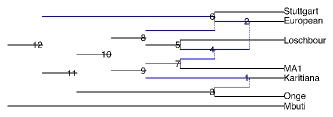
(a)

(b)

(c)

(d)

Figure 4: (a) Admixture graph $N$ from [Lazaridis et al., 2014, Fig. 3] with $h=4$ reticulations (hybrid edges are coloured). $N$ has one non-trivial biconnected component (blob) $B$, induced by all its internal nodes except for the root. $B$ contains all 4 reticulations so $N$ has level $\ell=4$. (b)-(d) Various cluster graphs for the moralized blob $B^{m}$: (b) clique tree, (c) join-graph structuring with the maximum cluster size set to 3, (d) LTRIP using the set of node families in $B$. Here sepsets (not shown) are the intersection of their incident clusters, and are small with 1 node only in (c) and (d). Purple boxes and edges: clusters and sepsets that contain node 8. Red text: hybrid families.

5.1 Calibration

Updating beliefs on a loopy cluster graph uses Algorithm 1 in the same way as on a clique tree. A cluster graph is said to be calibrated when its normalized beliefs have converged (i.e. are unchanged by Algorithm 1 along any edge). For calibration, neighboring clusters $\mathcal{C}_{i}$ and $\mathcal{C}_{j}$ must have beliefs that are marginally consistent over the variables in their sepset $\mathcal{S}_{i,j}$:

$$\int\beta_{i}d(\mathcal{C}_{i}\!\setminus\!\mathcal{S}_{i,j})=\tilde{\mu}_{i\rightarrow j}\propto\mu_{i,j}\propto\tilde{\mu}_{j\rightarrow i}=\int\beta_{j}d(\mathcal{C}_{j}\!\setminus\!\mathcal{S}_{i,j})\;.$$

On a clique tree, calibration can be guaranteed at the end of a finite sequence of messages passed. Clique and sepset beliefs are then proportional to the posterior distribution over their variables, and can be integrated to compute the common normalization constant $\kappa=\kappa_{i}\left(=\int\beta_{i}d\mathcal{C}_{i}\right)=\kappa_{j,k}\left(=\int\mu_{j,k}d\mathcal{S}_{j,k}\right)$, which equals the likelihood. For loopy BP, calibration is not guaranteed. If it is attained, then we can similarly view cluster and sepset beliefs as unnormalized approximations of the posterior distribution over their variables, though the $\kappa_{i}$s and $\kappa_{j,k}$s may differ, grow unboundedly, and generally do not equal or estimate the likelihood. Gaussian models enjoy the remarkable property that, if calibration can be attained on a cluster graph, then the approximate posterior means (ancestral values) are guaranteed to be exact. In contrast, the posterior variances are generally inexact, and are typically underestimated Weiss and Freeman [1999], Wainwright et al. [2003], Malioutov et al. [2006], although we found them overestimated in our phylogenetic examples below (Fig. 7).

Successful calibration depends on various aspects such as the features of the loops in the cluster graph, the factors in the model, and the scheduling of messages. For beliefs to converge, a proper message schedule requires that a message is passed along every sepset, in each direction, infinitely often (until stopping criteria are met) Malioutov et al. [2006]. Multiple scheduling schemes have been devised to help reach calibration more often and more accurately. These can be data-independent (e.g. choosing a list of trees nested in the cluster graph that together cover all clusters and edges, then iteratively traversing each tree in both directions Wainwright et al. [2003]) or adaptive (e.g. prioritizing messages between clusters that are further from calibration Elidan et al. [2006], Sutton and McCallum [2007], Knoll et al. [2015], Aksenov et al. [2020]).

5.2 Likelihood approximation

To approximate the log-likelihood $\operatorname{LL}(\theta)=\log\int p_{\theta}(x)dx$ from calibrated beliefs on cluster graph $\mathcal{U}^{*}=({\cal V}^{*},{\cal E}^{*})$, denoted together as $q=\{\beta_{i},\mu_{i,j};{\cal C}_{i}\in{\cal V}^{*},\{{\cal C}_{i},{\cal C}_{j}\}\in{\cal E}^{*}\}$, we can use the factored energy functional Koller and Friedman [2009]:

$$\tilde{F}(p_{\theta},q)=\sum_{\mathcal{C}_{i}\in\mathcal{V}^{*}}\!\operatorname{E}_{\beta_{i}}(\log\psi_{i})+\!\sum_{\mathcal{C}_{i}\in\mathcal{V}^{*}}\!\mathrm{H}(\beta_{i})-\!\!\!\!\!\!\sum_{\{\mathcal{C}_{i},\mathcal{C}_{j}\}\in\mathcal{E}^{*}}\!\!\!\!\!\!\mathrm{H}(\mu_{i,j})\;.$$ (8)

Recall that $\psi_{i}$ is the product of factors $\phi_{v}$ assigned to cluster ${\cal C}_{i}$. Here $\operatorname{E}_{\beta_{i}}$ denotes the expectation with respect to $\beta_{i}$ normalized to a probability distribution. $\mathrm{H}(\beta_{i})$ and $\mathrm{H}(\mu_{i,j})$ denote the entropy of the distributions defined by normalizing $\beta_{i}$ and $\mu_{i,j}$ respectively. $\tilde{F}(p_{\theta},q)$ has the advantage of involving local integrals that can be calculated easily: each over the scope of a single cluster or sepset. The justification for $\tilde{F}(p_{\theta},q)$ comes from two approximations. First, following the expectation-maximization (EM) decomposition, $\operatorname{LL}(\theta)$ can be approximated by the evidence lower bound (ELBO) used for variational inference Ranganath et al. [2014]. For any distribution $q$ over the full set of variables, which are here the unobserved (latent) variables after absorbing evidence from the data, we have

$$\operatorname{LL}(\theta)\geq\operatorname{ELBO}(p_{\theta},q)=\operatorname{E}_{q}(\log p_{\theta})+H(q)\;.$$

The gap $\operatorname{LL}(\theta)-\operatorname{ELBO}(p_{\theta},q)$ is the Kullback-Leibler divergence between $q$, and $p_{\theta}$ normalized to the distribution of the unobserved variables conditional on the observed data. The first approximation comes from minimizing this gap over a class of distributions $q$ that does not necessarily include the true conditional distribution. The second approximation comes from pretending that for a given distribution $q$ with a belief factorization

$$q\propto\frac{\prod_{\mathcal{C}_{i}\in\mathcal{V}^{*}}\beta_{i}}{\prod_{\{\mathcal{C}_{i},\mathcal{C}_{j}\}\in\mathcal{E}^{*}}\mu_{i,j}}\;,$$

its marginal over a given cluster (or a given sepset) is equal to the normalized belief of that cluster (or sepset), simplifying $\operatorname{E}_{q}(\log\psi_{i})$ to $\operatorname{E}_{\beta_{i}}(\log\psi_{i})$ and simplifying $\operatorname{E}_{q}(-\log\beta_{i})$ to $\mathrm{H}(\beta_{i})$. This simplification leads to the more tractable $\tilde{F}(p_{\theta},q)$, in which each integral is of lower dimension, within the scope of a single cluster or sepset.

5.3 Scalability versus accuracy: choice of cluster graph complexity

5.3.1 Scalability, treewidth and phylogenetic network complexity

At the cost of exactness, loopy cluster graphs can offer greater computational scalability than clique trees because they allow for smaller cluster sizes, which reduces the complexity associated with belief updates. For example, consider a Gaussian model for $p$ traits: $\dim(x_{v})=p$ at all nodes $v$ in the network. For a clique tree $\mathcal{U}$ with $m$ cliques and maximum clique size $k$, passing a message between neighbor cliques has complexity $\mathcal{O}(p^{3}k^{3})$ and calibrating $\mathcal{U}$ has complexity $\mathcal{O}(mp^{3}k^{3})$. Now consider a cluster graph $\mathcal{U}^{*}$ with $m^{*}$ clusters, $\mathcal{O}(m^{*})$ edges, and maximum cluster size $k^{*}<k$. Then passing a message between neighbor cliques of $\mathcal{U}^{*}$ has complexity $\mathcal{O}(p^{3}{k^{*}}^{3})$ so it is faster than on $\mathcal{U}$. But calibrating $\mathcal{U}^{*}$ now requires more belief updates because each edge needs to be traversed more than twice. If each edge is traversed in both directions $b$ times to reach convergence, then calibrating $\mathcal{U}^{*}$ has complexity $\mathcal{O}(bm^{*}p^{3}{k^{*}}^{3})$. So if $\mathcal{U}^{*}$ has smaller clusters than $\mathcal{U}$ and if $(k/k^{*})^{3}\gg bm^{*}/m$, then loopy BP on $\mathcal{U}^{*}$ runs faster than BP on $\mathcal{U}$. Loopy BP could be particularly advantageous for complex networks whose clique trees have large clusters.

Cluster graph construction determines the balance between scalability and approximation quality. At one end of the spectrum, the most scalable and least accurate are the factor graphs, also known as Bethe cluster graphs Yedidia et al. [2005]. A factor graph has one cluster per factor $\phi_{v}$ and one cluster per variable, and so has the smallest possible maximum clique size $k^{*}$ and each sepset reduced to a single variable. Various algorithms have been proposed for constructing cluster graphs along the spectrum (e.g. LTRIP Streicher and du Preez [2017]) (Fig. 4). Notably, join-graph structuring Mateescu et al. [2010] spans the whole spectrum because it is controlled by a user-defined maximum cluster size $k^{*}$, which can be varied from its smallest possible value to a value large enough to obtain a clique tree.

At the other end of the spectrum, the best maximum clique size $k$ is $1+\operatorname{tw}(G^{m})$, where $\operatorname{tw}(G^{m})$ is the treewidth of the moralized graph. Loopy BP becomes interesting when $\operatorname{tw}(G^{m})$ is large, making exact BP costly. Unfortunately, determining the treewidth of a general graph is NP-hard Arnborg et al. [1987], Bodlaender and Koster [2010]. Heuristics such as greedy minimum-fill or nested dissection Strasser [2017], Hamann and Strasser [2018] can be used to obtain clique trees whose maximum clique size $k$ is near the optimum $1+\operatorname{tw}(G^{m})$.

Different cluster graph algorithms could potentially be applied to the different biconnected components, or blobs Gusfield et al. [2007] (e.g. LTRIP for one blob, clique tree for another), perhaps based a blob’s attributes that are easy to compute. To choose between loopy versus exact BP, or between different cluster graph constructions more generally, one could use traditional complexity measures of phylogenetic networks as potential predictors of cost-effectiveness. For example, the reticulation number $h$ is straightforward to compute. In a binary network, where all internal non-root nodes have degree 3, $h$ is simply the number of hybrid nodes. More generally $h=|\{\mbox{hybrid edges}\}|-|\{\mbox{hybrid nodes}\}|$ Van Iersel et al. [2010]. The level of a network is the maximum reticulation number within a blob Gambette et al. [2009]. The network’s level ought to predict treewidth better than $h$ because a graph’s treewidth equals the maximum treewidth of its blobs Bodlaender [1998], and moralizing the network does not affect its nodes’ blob membership. These phylogenetic complexity measures do not predict treewidth perfectly Scornavacca and Weller [2022] except in simple cases as shown below, proved in SM section B.

Proposition 1.

Let $N$ be a binary phylogenetic network with $h$ hybrid nodes, level $\ell$, and let $t$ be the treewidth of the moralized network $N^{m}$ obtained from $N$. For simplicity, assume that $N$ has no parallel edges and no degree-2 nodes other than the root.

1. If $\ell=0$ then $h=0$ and $t=1$.

2. If $\ell=1$ then $h\geq 1$ and $t=2$.

3. Let $v_{1}$ be a hybrid node with non-adjacent parents $u_{1},u_{2}$. If $v_{1}$ has a descendant hybrid node $v_{2}$ such that one of its parents is not a descendant of either $u_{1}$ or $u_{2}$, then $\ell\geq 2$ and $t\geq 3$.

Figure 5: Two binary networks with a hybrid ladder and $h=\ell=2$. $N_{1}$ satisfies (A2) of Proposition 1 and $N_{1}^{m}$ has treewidth $t=3$. $N_{2}$ does not meet (A2) (see red/purple annotations) and $N_{2}^{m}$ has treewidth $t=2$. Stacking more hybrid ladders in the same way above $a$ and $b$ increases $h$ and $\ell$ but leaves $N_{2}^{m}$ outerplanar, keeping $t=2$.

Level-1 networks have received much attention in phylogenetics because they are identifiable under various models under some mild restrictions Solís-Lemus and Ané [2016], Baños [2019], Gross et al. [2021], Xu and Ané [2023]. Several inference methods limit the search to level-1 networks Solís-Lemus and Ané [2016], Oldman et al. [2016], Allman et al. [2019], Kong et al. [2022]. Since moralized level-1 networks have treewidth 2, exact BP is guaranteed to be efficient on them.

Beyond level-1, a network has a hybrid ladder (also called stack Semple and Simpson [2018]) if a hybrid node $v_{1}$ has a hybrid child node $v_{2}$. By Proposition 1, a hybrid ladder has the potential to increase treewidth of the moralized network and decrease BP scalability, if the remaining conditions in (A2) are met. Related results in Chaplick et al. [2023] are for undirected graphs that do not require prior moralization, and contain ladders defined as regular $2\times L$ grids. Their Observation 1, that a graph containing a non-disconnecting grid ladder of length $L\geq 2$ has treewidth at least 3, relies on a similar argument as for (A2). However, structures leading to the conditions in (A2) are more general, even before moralization. It may be interesting to extend some of the results from Chaplick et al. [2023] to moralized hybrid ladders in rooted networks.

In Fig. 5 (right) $N_{2}$ has a hybrid ladder that does not meet all conditions of (A2), and has $t=2$. Generally, outerplanar networks have treewidth at most $2$ Bodlaender [1998], and if bicombining (hybrid nodes have exactly 2 parents), remain outerplanar after moralization. Networks in which no hybrid node is the descendant of another hybrid node in the same blob are called galled networks Huson et al. [2010]. They provide more tractability to solve the cluster containment problem Huson et al. [2009]. Here, galled networks would then never meet the assumptions of (A2) and it would be interesting to study their treewidth after moralization.

We performed an empirical investigation of how $h$ and $\ell$ can predict the treewidth $t$ of the moralized network. Fig. 6 shows that $t$ correlates with $h$ and $\ell$, on networks estimated from real data using various inference methods and on networks simulated under the biologically realistic birth-death-hybridization model Justison and Heath [2024], Justison et al. [2023], especially for complex networks. For networks with hundreds of tips (Thorson et al. [2023] lists several studies of this size), large maximum clique sizes $k\geq 30$ are not uncommon. In contrast, a Bethe cluster graph would have maximum cluster size $k^{*}=3$, so that $(k/k^{*})^{3}\geq 10^{3}$ would provide a large computational gain for loopy BP to be considered.

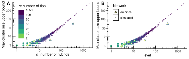
Figure 6: We observe a positive sublinear relationship between a maximum clique size upperbound (from the greedy minfill heuristic) and the number of hybrids (A) or network level (B) on a combined sample of 11 empirical networks and 2509 simulated birth-death-hybridization networks. The empirical networks were sampled from [Maier et al., 2023, Figs. 3a-c (left), 4a-c (left)] (reported as estimated by Bergström et al. [2020], Librado et al. [2021], Hajdinjak et al. [2021], Lipson et al. [2020], Wang et al. [2021], Sikora et al. [2019]), [Lazaridis et al., 2014, Fig. 3], [Nielsen et al., 2023, Fig. 3 (left)], [Sun et al., 2023, Fig. 4c], [Müller et al., 2022, Fig. 1a], [Neureiter et al., 2022, Fig. 5a]; fit by these authors using ADMIXTOOLS Patterson et al. [2012], Maier et al. [2023], admixturegraph Leppälä et al. [2017], OrientAGraph Molloy et al. [2021], contacTrees Neureiter et al. [2022], Recombination Müller et al. [2022], AdmixtureBayes Nielsen et al. [2023]. The simulated networks were obtained by subsampling 10 networks per parameter scenario simulated by Justison and Heath [2024], then filtering out networks of treewidth 1 (trees, possibly with parallel hybrid edges).

5.3.2 Approximation quality with loopy BP

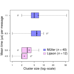
Figure S3: Boxplots (with means as points) showing the distribution of cluster sizes in the join-graph structuring cluster graph $\mathcal{U}^{*}$ and in the clique tree $\mathcal{U}$ from Fig. 7. The factor graph has clusters of size between 1 and 3 (not displayed). The time for 100 iterations (defined in Fig. 7) was benchmarked over 20 replicates on a MacBook Pro M2 2022, and divided by the number of messages per 100 iterations to obtain an estimate of the mean time per belief update (vertical axis).

We simulated data on a complex graph (40 tips, 361 hybrids) [Müller et al., 2022, Fig. 1a] and a simpler graph (12 tips, 12 hybrids) [Lipson et al., 2020, Extended Data Fig. 4], then compared estimates from exact and loopy BP. For both networks, edges of length 0 were assigned the minimum non-zero edge length after suppressing any non-root degree-2 nodes. Trait values $\mathrm{\mathbf{x}}=(\mathrm{x}_{1},\dots,\mathrm{x}_{n})$ at the tips were simulated from a BM with rate $\sigma^{2}=1$ and $\mathrm{x}_{\rho}=0$ at the root. Figure 7 shows the exact and approximate log-likelihood and conditional mean and variance of $x_{\rho}$ assuming a BM with rate $\sigma^{2}=1$ but improper prior $x_{\rho}\sim\mathcal{N}(0,\infty)$, using a greedy minimum-fill clique tree $\mathcal{U}$ and a cluster graph $\mathcal{U}^{*}$. Using a factor graph, calibration failed for the complex network (SM section C, Fig. S2), so we used join-graph structuring to build $\mathcal{U}^{*}$. $\mathcal{U}$ can be calibrated in one iteration and the calculated quantities are exact (horizontal lines). In contrast, $\mathcal{U}^{*}$ requires multiple passes and gives approximations. Calibration required more iterations on the complex network ($h=361$) than on the simpler network ($h=11$), as expected. But for both networks, the factored energy (8) approximated the log-likelihood very well. The distribution of the root state $x_{\rho}$ conditional on the data seems more difficult to approximate. The conditional mean was correctly estimated but required more iterations than the log-likelihood approximation on the complex network. The conditional variance was severely overestimated on the complex network and very slightly overestimated on the simpler network. As desired, the average computing time per belief update was lower on $\mathcal{U}^{*}$, although modestly so due to the clique tree $\mathcal{U}$ having many small clusters of size similar to those in $\mathcal{U}^{*}$ (Fig. S3).

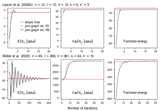
Figure 7: Accuracy of loopy BP. Approximation of the conditional distribution of the root state $X_{\rho}$ (left and center) and log-likelihood (right) using a greedy minimum-fill clique tree $\mathcal{U}$ and a join-graph structuring cluster graph $\mathcal{U}^{*}$ for two networks of varying complexity Müller et al. [2022], Lipson et al. [2020] as measured by their number of tips ($n$), level ($\ell$), number of hybrids ($h$), maximum clique size ($k$), and maximum cluster size ($k^{*}$). For $\mathcal{U}$, estimates are exact after one iteration and shown as horizontal red lines. For $\mathcal{U}^{*}$, estimates are shown over 20 (first row), 50 or 200 (second row) iterations. Each iteration consists of two passes through each spanning tree in a minimal set that jointly covers $\mathcal{U}^{*}$. In each plot, the two curves correspond to two different regularizations of initial beliefs (SM section E, dotted: algorithm R1, solid: algorithm R2).

6 Leveraging BP for efficient parameter inference

6.1 BP for fast likelihood computation

In some particularly simple models, such as the BM on a tree, fast algorithms such as IC Felsenstein [1985] or phylolm Ho and Ané [2014] can directly calculate the best-fitting parameters that maximize the restricted likelihood (REML), in a single tree traversal avoiding numerical optimization. For more general models, such closed-form estimates are not available. One product of BP is the likelihood of any fixed set of model parameters. BP can hence be simply used as a fast algorithm for likelihood computation, which can then be exploited by any statistical estimation technique, in a Bayesian or frequentist framework. Most of the tools cited in section 2.3 use either direct numerical optimization of the likelihood Mitov et al. [2019], Boyko et al. [2023], Bartoszek et al. [2023] or sampling techniques such as Markov Chain Monte Carlo (MCMC) Pybus et al. [2012], FitzJohn [2012] for parameter inference.

BP also outputs the trait distribution at internal, unobserved nodes conditioned on the observed data at the tips. In addition to providing a tool for efficient ancestral state reconstruction, these conditional means and variances can be used for parameter inference, with approaches based on latent variable models such as Expectation Maximization (EM) Bastide et al. [2018a], or Gibbs sampling schemes Cybis et al. [2015]. Although not currently used in the field of evolutionary biology to our knowledge, approaches based on approximate EM algorithms Heskes et al. [2003] and relying on loopy BP could also be used.

6.2 BP for fast gradient computation

As we show below, the conditional means and variances at ancestral nodes can be used to efficiently compute the gradient of the likelihood Salakhutdinov et al. [2003]. The gradient of the likelihood can help speed up inference in many different statistical frameworks Barber [2012]. In a phylogenetic context, gradients have been used to improve maximum likelihood estimation Ji et al. [2020], Bayesian estimation through Hamiltonian Monte Carlo (HMC) approaches Zhang et al. [2021], Fisher et al. [2021], Bastide et al. [2021], or variational Bayes approximations Fourment and Darling [2019]. Although automatic differentiation can be used on trees for some models Swanepoel et al. [2022], direct computations of the gradient using BP-like algorithms have been shown to be more efficient in some contexts Fourment et al. [2023]. After recalling Fisher’s identity to calculate gradients after BP calibration, we illustrate its use on the BM model (univariate or multivariate) where it allows for the derivation of a new analytical formula for the REML parameter estimates.

6.2.1 Gradient Computation with Fisher’s Identity

In a phylogenetic context, latent variables are usually internal nodes, while observed variables are leaves. We write $Y=\mathopen{\{}X_{v,j}:\text{trait }j\text{ observed at }v\in V\mathclose{\}}$ the set of observed variables. Fisher’s identity provides a way to link the gradient of the log-likelihood of the data $\operatorname{LL}(\theta)=\log p_{\theta}(Y)$ at parameter $\theta$, with the distribution of all the variables conditional on the observations $Y$. We refer to [Cappé et al., 2005, chap. 10] or [Barber, 2012, chap. 11] for general introductions on Markov models with latent variables. Under broad assumptions, Fisher’s identity states (see Proposition 10.1.6 in Cappé et al. [2005], or Section 11.6 in Barber [2012]):

$$\left.\nabla_{\theta^{\prime}}\left[\log p_{\theta^{\prime}}(Y)\right]\right|_{\theta^{\prime}=\theta}=\operatorname{E}_{\theta}\left[\left.\left.\nabla_{\theta^{\prime}}\left[\log p_{\theta^{\prime}}(X_{v};v\in V)\right]\right|_{\theta^{\prime}=\theta}\mathrel{}\middle|\mathrel{}Y\right.\right],$$

where $\left.\nabla_{\theta^{\prime}}[f(\theta^{\prime})]\right|_{\theta^{\prime}=\theta}$ denotes the gradient of $f$ with respect to the generic parameters $\theta^{\prime}$ and evaluated at $\theta^{\prime}=\theta$, and $\operatorname{E}_{\theta}[\left.\bullet\mathrel{}\middle|\mathrel{}Y\right.]$ the expectation conditional on the observed data under the model parametrized by $\theta$, which is precisely where the output from BP can be used. Plugging in the factor decomposition from the graphical model (4) we get:

$$\left.\nabla_{\theta^{\prime}}\left[\log p_{\theta^{\prime}}(Y)\right]\right|_{\theta^{\prime}=\theta}=\sum_{v\in V}\operatorname{E}_{\theta}\left[\left.\left.\nabla_{\theta^{\prime}}\left[\log\phi_{v}(X_{v}|X_{u},\theta^{\prime};u\in\operatorname{pa}(v))\right]\right|_{\theta^{\prime}=\theta}\mathrel{}\middle|\mathrel{}Y\right.\right].$$ (9)

While (9) applies to the full vector of all model parameters, it can also be applied to take the gradient with respect to a single parameter $\theta$ of interest, keeping the other parameters fixed. For instance, we can focus on one rate matrix $\bm{\Sigma}$ of a BM model, or one primary optimum of an OU model. Special care needs to be taken for gradients with respect to structured matrices, such as variance matrices that need to be symmetric (see e.g. Bastide et al. [2021]) or with a sparse inverse under structural equation modeling for high dimentional traits Thorson and van der Bijl [2023].

For models where the conditional expectation of the factor in (9) has a simple form, this formula is the key to an efficient gradient computation. In particular, for discrete traits as in Example 2, the expectation becomes a sum of a manageable number of terms, local to a cluster, weighted by the normalized cluster belief after calibration [Koller and Friedman, 2009, ch. 19].

6.2.2 Gradient computation for linear Gaussian models

For linear Gaussian models (2), log-factors can be written as quadratic forms (6), so their derivatives have analytical formulas (see SM section D). The conditional expectation in (9) then only depends on the joint first and second order moments of the variables $(X_{v},X_{\operatorname{pa}(v)})$ in a cluster, which are known as soon as the beliefs are calibrated. When the graph is a tree, Bastide et al. [2021] exploited this formula to derive gradients in the general linear Gaussian case. However, they did not use the complete factor decomposition (4), but instead an ad-hoc decomposition that only works when the graph is a (binary) tree, and exploits the split partitions defined by the tree. In contrast, the present approach gives a recipe for the efficient gradient computation of any linear Gaussian model on any network, as soon as beliefs are calibrated.

In the special case where the process is a homogeneous BM (univariate or multivariate) on a network with a weighted-average merging rule (3), a constant rate $\bm{\Sigma}$, no missing data at the tips, and, if present, within-species variation that is proportional to $\bm{\Sigma}$, then the gradient with respect to $\bm{\Sigma}$ takes a particularly simple form. Setting this gradient to zero, we find an analytical formula for the REML estimate of $\bm{\Sigma}$ and for the ML estimate of the ancestral mean $\mu_{\rho}$ (SM section D.3). In a phylogenetic regression setting, a similar formula can be found for the ML estimate of coefficients (SM section D.4). Efficient algorithms such as IC and phylolm already exist to compute these quantities on a tree, in a single traversal. Here, our formulas need two traversals but remain linear in the number of tips, and because they rely on a general BP formulation, they apply to networks with reticulations. Fisher’s identity and BP hence offer a general method for gradient computation, and could lead to analytical formulas for other simple models. Such efficient formulas could alleviate numerical instabilities observed in software such as mvSLOUCH, which experienced a significant failure rate for the BM on trees with a large number of traits Bartoszek et al. [2024].

6.2.3 Hessian computation with Louis’s identity

Using similar techniques, the Hessian of the log-likelihood with respect to the parameters can also be obtained as a conditional expectation of the Hessian of the complete log-likelihood:

$$\left.\left\{\nabla_{\theta^{\prime}}^{2}\left[\log p_{\theta^{\prime}}(Y)\right]+\nabla_{\theta^{\prime}}\left[\log p_{\theta^{\prime}}(Y)\right]\left[\nabla_{\theta^{\prime}}\left[\log p_{\theta^{\prime}}(Y)\right]\right]^{\top}\right\}\right|_{\theta^{\prime}=\theta}=\\ \operatorname{E}_{\theta}\left[\left.\big{\{}\nabla_{\theta^{\prime}}^{2}\left[\log p_{\theta^{\prime}}(X_{v};v\in V)\right]+\nabla_{\theta^{\prime}}\left[\log p_{\theta^{\prime}}(X_{v};v\in V)\right]\left[\nabla_{\theta^{\prime}}\left[\log p_{\theta^{\prime}}(X_{v};v\in V)\right]\right]^{\top}\big{\}}|_{\theta^{\prime}=\theta}\mathrel{}\middle|\mathrel{}Y\right.\right].$$

This so-called Louis identity Cappé et al. [2005] also simplifies under the factor decomposition (4), and leads to tractable formulas in simple Gaussian or discrete cases.

6.3 BP for direct Bayesian parameter inference

Likelihood or gradient-based approaches require careful analytical computations to get exact formulas in any new model within the class of linear Gaussian graphical models, depending on the parameters of interest Bastide et al. [2021]. One way to alleviate this problem is to use a Bayesian framework, and expand the graphical model to include both the phylogenetic network and the evolutionary parameters, which are seen as random variables themselves, as e.g., in Höhna et al. [2014]. Then, inferring parameters amounts to learning their conditional distribution in this larger graphical model. In this setting, the output of interest from BP is not the likelihood but the distribution of random variables (evolutionary parameters primarily) conditional on the observed data.

Exact computation may not be possible in this extended graphical model, because it is typically not linear Gaussian and the graph’s treewidth can be much larger than that of the phylogenetic network, when one parameter (e.g. the evolutionary rate) affects multiple node families. Therefore, approximations may need to be used. For example, “black box” optimization techniques rely on variational approaches to reach a tractable approximation of the posterior distribution of model parameters Ranganath et al. [2014]. The conditional distribution of unobserved variables, provided by BP, facilitates the noisy approximation of the variational gradient that can be used to speed up the optimization of the variational Bayes approximation.

7 Challenges and Extensions

7.1 Degeneracy

While our implementation provides a proof-of-concept, various technical challenges still need to be solved. Much of the literature on BP focuses on factor graphs, which failed to converge for one of our example phylogenetic networks. More work is needed to better understand the convergence and accuracy of alternative cluster graphs, and on other choices that can substantially affect loopy BP’s efficiency, such as scheduling. Below, we focus on implementation challenges due to degeneracies.

For the message $\tilde{\mu}_{i\rightarrow j}$ to be well-defined in step 1 of Gaussian BP, the belief of the sending cluster must have a precision matrix $\bm{K}$ in (6) with a full-rank submatrix with respect to the variables to be integrated out ($\bm{K}_{I}$ in Algorithm 2). This condition can fail under realistic phylogenetic models, due to two different types of degeneracy.

The first type arises from deterministic factors: when $\bm{V}_{v}=0$ in (2) and $X_{v}$ is determined by the states at parent nodes $X_{\operatorname{pa}(v)}$ without noise, e.g. when all of $v$’s parent branches have length 0 in standard phylogenetic models. This is expected at hybridization events when both parents have sampled descendants in the phylogeny, because the parents and hybrid need to be contemporary of one another. This situation is also common in admixture graphs Maier et al. [2023] due to a lack of identifiability of hybrid edge lengths from $f$ statistics, leading to a “zipped-up” estimated network in which the estimable composite length parameter is assigned to the hybrid’s child edge Xu and Ané [2023]. With this degeneracy, $X_{v}$ has infinite precision given its parents, that is, $\bm{K}$ has some infinite values. The complications are technical, but not numerical. For example, one can use a generalized canonical form that includes a Dirac distribution to capture the deterministic equation of $X_{v}$ given $X_{\operatorname{pa}(v)}$ from (2). Then BP operations need to be extended to these generalized canonical forms, as done in Schoeman et al. [2022] (illustrated in SM section F). One could also modify the network by contracting internal tree edges of length 0. At hybrid nodes, adding a small variance to $\bm{V}_{v}$ would be an approximate yet biologically realistic approach.

The second type of degeneracy arises when the precision submatrix $\bm{K}_{I}$ is finite but not of full rank. In phylogenetic models, this is frequent at initialization (5). For example, consider a cluster of 3 nodes: a hybrid $v$ and its 2 parents. By (7) we see that $\operatorname{rank}(\bm{K}_{v})\leq p$. So at initialization with belief $\phi_{v}$, $\bm{K}_{I}$ is degenerate if we seek to integrate out $|I|=2$ nodes, which would occur if the cluster is adjacent to a sepset containining only one parent of $v$. This situation is typical of factor graphs. Initial beliefs would also be degenerate with $\bm{K}=\bm{0}$ for any cluster that is not assigned any factor by (5). This may occur if there are more clusters than node families, or if the graph has nested redundant clusters (e.g. from join-graph structuring). In some cases, a schedule may avoid these degeneracies, guaranteeing a well-defined message at each BP update. On a clique tree, a schedule based on a postorder traversal has this guarantee, provided that all $p$ traits are observed at all leaves or that trait $j$ at node $v$ is removed from scope if it is unobserved at all its descendants. But generally, it is unclear how to find such a schedule. Another approach is to simply skip a BP update if its message is ill-defined, though there is no guarantee that the sending cluster will eventually have a well-behaved belief to pass the message later. A robust option is to regularize cluster beliefs, right after initialization (5) or during BP, by increasing some diagonal elements of $\bm{K}$ to make $\bm{K}_{I}$ of full rank. To maintain the probability model, this cluster belief regularization is balanced by a similar modification to a corresponding sepset. SM section E describes two such approaches that appear to work well in practice, although theoretical guarantees have not been established.

7.2 Loopy BP is promising for discrete traits

We focused on Gaussian models in this paper, for which the ‘lazy’ matrix approach is polynomial. For discrete trait models, the computational gains from loopy BP can be much greater, because alternative approaches are not polynomial on general networks. For a trait with $c$ states ($c=2$ for a binary trait as in Example 2), passing a message has complexity $\mathcal{O}(c^{k})$ where $k$ is the sending cluster size. Thus, cluster graphs with small clusters can bring exponential computational gains. Even exact BP can bring significant computational gains to existing approaches that rely on other means to reduce complexity. For example, the model without ILS used in Lutteropp et al. [2022], Allen-Savietta [2020] is a mixture model, so the network likelihood can be calculated as a weighted average of tree likelihoods for which exact BP takes linear time. This approach scales exponentially with $h$ because there are typically $\mathcal{O}(2^{h})$ trees displayed in a network. In contrast, the complexity of BP on a clique tree of maximum clique size $k$ is $\mathcal{O}(nc^{k})$, thus parametrized by the treewidth $t$ of the moralized network instead of $h$ ($t=k-1$ for an optimal clique tree). Given our empirical evidence that $t$ grows more slowly than $h$ or the network’s level $\ell$ in biologically-realistic networks (Fig. 6), exact BP could achieve significant computational gains and loopy BP substantially more.

A BP approach is already used in momi2 Kamm et al. [2020], who use a clique tree built from a node ordering by age from youngest to oldest, to get conditional likelihoods of the derived allele count under a Moran model (without mutation). The mutation-with-ILS model in SnappNet can be also reframed as a graphical model on a graph expanded from the phylogenetic network (as shown in Example 3 and SM section A). Accordingly, the BP-like algorithm in Rabier et al. [2021] has complexity controlled by the network’s scanwidth, a parameter introduced by Berry et al. [2020]. Using regular BP on more optimal clique trees and loopy BP on cluster graphs may help speed up computations even more.

Also related is the algorithm in Scornavacca and Weller [2022], who use a clique tree to solve a parsimony problem. In this non-probabilistic setting, it is unclear how cluster graphs could be leveraged to speed up algorithms as they do in loopy BP.

To deal with computational intractability, the most widely-used probabilistic methods to infer networks from DNA sequences are based on composite likelihoods Solís-Lemus and Ané [2016], Yu and Nakhleh [2015] or summary statistics like $f$ statistics Maier et al. [2023], Nielsen et al. [2023], leading to a lack of identifiability for parts of the network topology and some of its parameters Solís-Lemus and Ané [2016], Baños [2019], Xu and Ané [2023], Ané et al. [2024], Allman et al. [2024], Rhodes et al. [2024]. These identifiability issues should be alleviated if using the full data becomes tractable thanks to exact or loopy BP.

Supplementary Material

Technical derivations are available in the Supplementary Material (SM). Code to reproduce Figures 4a, 6 and 7 is available at https://github.com/bstkj/graphicalmodels_for_phylogenetics_code. A julia package for Gaussian BP on phylogenetic networks is available at https://github.com/cecileane/PhyloGaussianBeliefProp.jl.

 

Supplementary material

 

Appendix A Recasting SnappNet as BP

SnappNet [Rabier et al., 2021] extends the model described in SNAPP [Bryant et al., 2012] to binary phylogenetic networks with reticulations. In the main text, their model is considered along a 2-taxon phylogenetic tree and Fig. 3b shows that the graphical model has a more complicated graph. The same applies in the presence of reticulations (see Fig. S1 for a 2-taxon phylogeny with 1 reticulation). In addition to the coalescent and speciation factors described in Example 3, we also need to describe hybridization factors. Consider an edge $e$ that is the child of a hybrid node, whose parent hybrid edges $p_{1}$ and $p_{2}$ have inheritance probabilities $\gamma_{1}$ and $\gamma_{2}$. The hybridization factors for the total allele count $\phi_{n_{\underline{p_{1}}}}=\mathbb{P}(n_{\underline{p_{1}}}\mid n_{\overline{e}})$ and $\phi_{n_{\underline{p_{2}}}}=\mathbbm{1}_{\{n_{\overline{e}}-n_{\underline{p_{1}}}\}}(n_{\underline{p_{2}}})$ describe a binomial distribution for each $n_{\underline{p_{i}}}$ ($i=1,2$) with $n_{\underline{p_{1}}}+n_{\underline{p_{1}}}=n_{\overline{e}}$, because each of the $n_{\overline{e}}$ individuals has a $\gamma_{i}$ chance of being assigned to edge $p_{i}$ ($i=1,2$). The hybridization factor for the red allele count is simply $\phi_{r_{\overline{e}}}=\mathbbm{1}_{\{r_{\underline{p_{1}}}+r_{\underline{p_{2}}}\}}(r_{\overline{e}})$ because $r_{\overline{e}}=r_{\underline{p_{1}}}+r_{\underline{p_{2}}}$.

Figure S1: (a) Phylogenetic network $N$ with hybrid edges in blue. (b) Graph $G$ for the graphical model associated with $N$. $G$ is a DAG with two roots ($\underline{1}$ and $\underline{2}$) and two leaves (${\color[rgb]{1,0,0}\underline{1}}$ and ${\color[rgb]{1,0,0}\underline{2}}$). (c) Clique tree $\mathcal{U}$ for $G$, with clusters $\mathcal{C}_{j}$ in grey and sepsets $\mathcal{S}_{i,j}$ in orange. To reduce clutter and simplify notations in this figure, $n_{\underline{e}}$ and $r_{\underline{e}}$ are both abbreviated as $\underline{e}$ and are distinguished by colours ($n$’s in black, $r$’s in red). Similarly, $n_{\overline{e}}$ and $r_{\overline{e}}$ are both denoted as $\overline{e}$ and distinguished by colours.

We show that applying the SnappNet algorithm to the network in Fig. S1(a) is equivalent to BP on the clique tree in Fig. S1(c). To start, we assign the initial beliefs $\phi_{n_{\overline{1}}}\phi_{r_{\underline{1}}}$ to cluster $\mathcal{C}_{1}$,   $\phi_{n_{\overline{2}}}\phi_{r_{\underline{2}}}$ to $\mathcal{C}_{4}$,   $\phi_{n_{\underline{\rho}}}\phi_{r_{\underline{\rho}}}\phi_{r_{\overline{5}}}\phi_{r_{\overline{4}}}$ to $\mathcal{C}_{7}$;   $\phi_{n_{\overline{5}}}\phi_{n_{\overline{3}}}\phi_{r_{\underline{5}}}\phi_{r_{\underline{3}}}$ to $\mathcal{C}_{3}$,   $\phi_{n_{\underline{4}}}\phi_{r_{\overline{3}}}\phi_{r_{\overline{2}}}$ to $\mathcal{C}_{5}$, and $\phi_{n_{\overline{4}}}\phi_{r_{\underline{4}}}$ to $\mathcal{C}_{6}$. Finally, all hybridization factors $\phi_{n_{\underline{5}}}\phi_{n_{\underline{3}}}\phi_{r_{\overline{1}}}$ are assigned to $\mathcal{C}_{2}$. Each sepset is assigned an initial belief of 1. The total allele counts $\mathrm{n}_{\underline{1}}$, $\mathrm{n}_{\underline{2}}$ (fixed by design) and the observed red allele counts $\mathrm{r}_{\underline{1}}$, $\mathrm{r}_{\underline{2}}$ at the tips are absorbed as evidence into the mutation factors $\phi_{r_{\underline{1}}}$, $\phi_{r_{\underline{2}}}$ and coalescent factors $\phi_{n_{\overline{1}}}$, $\phi_{n_{\overline{2}}}$ for the terminal edges. This is denoted as $\phi[\cdot]$, with $[\cdot]$ containing the evidence absorbed. BP messages are then passed on the clique tree from $\mathcal{C}_{1}$ and $\mathcal{C}_{4}$ (considered as leaves) towards $\mathcal{C}_{7}$ (considered as root) as follows:

$$\begin{split}\tilde{\mu}_{1\rightarrow 2}&=\phi_{n_{\overline{1}}}[\mathrm{n}_{\underline{1}}]\phi_{r_{\underline{1}}}[\mathrm{n}_{\underline{1}},\mathrm{r}_{\underline{1}}]=\mathrm{F}_{\overline{1}}(\mathcal{S}_{1,2})\\ \tilde{\mu}_{2\rightarrow 3}&=\sum_{\mathcal{C}_{2}\setminus\mathcal{S}_{2,3}}\phi_{n_{\underline{5}}}\phi_{n_{\underline{3}}}\phi_{r_{\overline{1}}}\cdot\tilde{\mu}_{1\rightarrow 2}=\mathrm{F}_{\underline{5},\underline{3}}(\mathcal{S}_{2,3})\\ \tilde{\mu}_{3\rightarrow 5}&=\sum_{\mathcal{C}_{3}\setminus\mathcal{S}_{3,5}}\phi_{n_{\overline{5}}}\phi_{n_{\overline{3}}}\phi_{r_{\underline{5}}}\phi_{r_{\underline{3}}}\cdot\tilde{\mu}_{2\rightarrow 3}=\mathrm{F}_{\overline{5},\overline{3}}(\mathcal{S}_{3,5})\\ \tilde{\mu}_{4\rightarrow 5}&=\phi_{n_{\overline{2}}}[\mathrm{n}_{\underline{2}}]\phi_{r_{\underline{2}}}[\mathrm{n}_{\underline{2}},\mathrm{r}_{\underline{2}}]=\mathrm{F}_{\overline{2}}(\mathcal{S}_{4,5})\\ \tilde{\mu}_{5\rightarrow 6}&=\sum_{\mathcal{C}_{5}\setminus\mathcal{S}_{5,6}}\phi_{n_{\underline{4}}}\phi_{r_{\overline{3}}}\phi_{r_{\overline{2}}}\cdot\tilde{\mu}_{3\rightarrow 5}\tilde{\mu}_{4\rightarrow 5}=\mathrm{F}_{\overline{5},\underline{4}}(\mathcal{S}_{5,6})\\ \tilde{\mu}_{6\rightarrow 7}&=\sum_{\mathcal{C}_{6}\setminus\mathcal{S}_{6,7}}\phi_{n_{\overline{4}}}\phi_{r_{\underline{4}}}\cdot\tilde{\mu}_{5\rightarrow 6}=\mathrm{F}_{\overline{5},\overline{4}}(\mathcal{S}_{6,7})\\ \beta_{7}^{\text{final}}&=\phi_{n_{\underline{\rho}}}\phi_{r_{\underline{\rho}}}\phi_{r_{\overline{5}}}\phi_{r_{\overline{4}}}\cdot\tilde{\mu}_{6\rightarrow 7}\\ \sum_{\mathcal{C}_{7}}\beta_{7}^{\text{final}}&=\sum_{\mathcal{C}_{7}\setminus\mathcal{S}_{6,7}}\phi_{r_{\underline{\rho}}}\sum_{\mathcal{S}_{6,7}}\phi_{n_{\underline{\rho}}}\phi_{r_{\overline{5}}}\phi_{r_{\overline{4}}}\cdot\tilde{\mu}_{6\rightarrow 7}=\sum_{\mathcal{C}_{7}\setminus\mathcal{S}_{6,7}}\phi_{r_{\underline{\rho}}}\mathrm{F}_{\underline{\rho}}(\mathcal{C}_{7}\setminus\mathcal{S}_{6,7})\end{split}$$

where the the $\mathrm{F}_{\mathbf{z}}$ functions are defined in Rabier et al. [2021] for different population interface sets $\mathbf{z}$ (each population interface is the top or bottom of some branch, e.g. $\overline{\rho}$, $\underline{\rho}$). That this correspondence does not always hold (e.g. suppose the messages were sent towards $\mathcal{C}_{1}$ instead), highlights that BP is more general. The $\mathrm{F}_{\mathbf{z}}$s recursively compose the likelihood according to rules described in Rabier et al. [2021], and can be expressed at the top-level as $\sum_{n_{\underline{\rho}},r_{\underline{\rho}}}\phi_{r_{\underline{\rho}}}\mathrm{F}_{\underline{\rho}}$. This is precisely the quantity from marginalizing $\beta^{\text{final}}_{7}$ above, the final belief of $\mathcal{C}_{7}$.

Appendix B Bounding the moralized network’s treewidth

Proof of Proposition 1.

Using the notations in the main text, let $N$ be as a binary phylogenetic network with $h$ hybrid nodes, level $\ell$, no parallel edges and no degree-2 nodes other than the root. Let $t$ be the treewidth of the moralized graph $N^{m}$ obtained from $N$.

(A0) is well-known: $t=1$ exactly when $N$ is a tree. If $\ell=1$ then $N$ has at least one non-trivial blob and every such blob is a cycle. So $N^{m}$ has outerplanar blobs and $t=2$ Biedl [2015], proving (A1).

Now consider hybrid nodes $v_{1}$ and $v_{2}$ as in (A2). Let $u_{3},u_{4}$ be the parents of $v_{2}$ such that $u_{3}$ is not a descendant of $u_{1}$ or $u_{2}$ (see Fig. 5, in which $u_{4}=v_{1}$). Then there must be a path $p_{4}$ from $v_{1}$ to $v_{2}$ through $u_{4}$ since $v_{2}$ is a descendant of $v_{1}$. For a directed path $p$, let $p^{u}$ denote the corresponding undirected path. Let $w$ be a strict common ancestor of $u_{1}$ and of $u_{2}$ such that there exist disjoint paths $p_{1}$, $p_{2}$, with $p_{i}$ from $w$ to $u_{i}$. Such $w$ exists because $u_{1}$ has a parent other than $u_{2}$ and vice versa. Let $C$ be the cycle in $N^{m}$ formed by concatenating $p^{u}_{1}$, $p^{u}_{2}$ and the moral edge $\{u_{1},u_{2}\}$. Next, pick any path $p$ from the root of $N$ to $u_{3}$. If $p$ does not share any node with $C$, then we can find a common ancestor $\tilde{w}$ of $w$ and $u_{3}$, and paths $p_{w}$ and $p_{3}$ from $\tilde{w}$ to $w$ and $u_{3}$ respectively, that do not intersect $p_{1}$ nor $p_{2}$. Then we can see that $N^{m}$ contains the complete graph on $\{w,u_{1},u_{2},v_{1}\}$ as a graph minor, by contracting $p^{u}_{w}+p^{u}_{3}+\{u_{3},v_{2}\}+p^{u}_{4}$ into a single edge between $w$ and $v_{1}$. If instead $p$ intersects $C$, then let $w^{\prime}$ be the lowest node at which $p$ and $C$ intersect. Then $w^{\prime}\neq u_{1}$ because otherwise $u_{3}$ would be its descendant. Similarly $w^{\prime}\neq u_{2}$. Let $p_{3}$ denote the subpath of $p$ from $w^{\prime}$ to $u_{3}$. Then $N^{m}$ contains the complete graph on $\{w^{\prime},u_{1},u_{2},v_{1}\}$ as a graph minor, as $C$ can be contracted into the cycle $\{w^{\prime},u_{1},u_{2}\}$ and $p^{u}_{3}+\{u_{3},v_{2}\}+p^{u}_{4}$ can be contracted into an edge $\{w^{\prime},v_{1}\}$. In both cases, $N^{m}$ contains the complete graph on 4 nodes as a graph minor, therefore its treewidth is $t\geq 3$ Bodlaender [1998]. Also, in both cases $v_{1}$ and $v_{2}$ are in a common undirected cycle in $N$, so in the same blob and $\ell\geq 2$. ∎

Appendix C Approximation quality with loopy BP

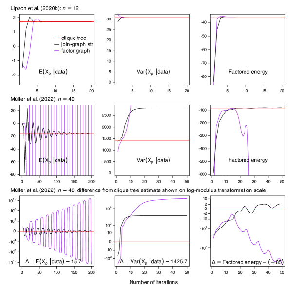
Figure S2: Comparing the accuracy of loopy BP between different cluster graphs: built from join-graph structuring $\mathcal{U}^{*}$ as in Fig. 7 (black), or a factor graph (purple). For both, initial beliefs are regularized using algorithm R4. The true values, obtained using a clique tree, are shown in red. The plots in the first row are for the simpler phylogenetic network, and the plots in the other rows are for the complex phylogeny. The last row shows the difference $\Delta$ between the loopy BP estimate and the true value, displayed on the log-modulus scale using the transformation $\mbox{sign}(\Delta)\log(1+|\Delta|)$. For the simpler phylogenetic network, convergence speed and accuracy are similar between $\mathcal{U}^{*}$ and the factor graph, which is unsurprising given their similarly small cluster sizes ($\leq 3$). For the complex network, the factor graph did not reach calibration as its iterates diverged for the conditional mean and factored energy.

Appendix D Gradient and parameter estimates under the BM

D.1 The homogeneous BM model

We consider here the simple case of a multivariate BM of dimension $p$ on a network: with $\bm{V}_{v}=\ell(e)\bm{\Sigma}$ at a tree node $v$ with parent edge $e$. At a hybrid node, we assume a weighted average merging rule as in (3.2) with a possible extra hybrid variance proportional to $\bm{\Sigma}$: $\widetilde{\bm{V}}_{h}=\widetilde{\ell}(h)\bm{\Sigma}$ for some scalar $\widetilde{\ell}(h)\geq 0$. To simplify equations, we define $\widetilde{\ell}(v)=0$ if $v$ is a tree node. Then for each node $v\in V$ the Gaussian linear model (3.1) simplifies to:

$$\left.X_{v}\mathrel{}\middle|\mathrel{}X_{\operatorname{pa}(v)}\right.\sim\mathcal{N}\left(\sum_{u\in\operatorname{pa}(v)}\gamma_{uv}X_{u};\;\ell(v)\bm{\Sigma}\right),$$ (SM-1)

with $\gamma_{uv}$ the inheritance probability associated with the branch going from $u$ to $v$, and

$$\ell(v)=\widetilde{\ell}(v)+\sum_{u\in\operatorname{pa}(v)}\gamma_{uv}^{2}\ell(e_{u\to v})\;.$$

At the root, we assume a prior variance proportional to $\bm{\Sigma}$: $X_{\rho}\sim\mathcal{N}\left(\mu_{\rho};\;\ell(\rho)\bm{\Sigma}\right)$ which may be improper (and degenerate) with infinite variance $\ell(\rho)=\infty$ or $\ell(\rho)=0$.

This model can also accommodate within-species variation, by considering each individual as one leaf in the phylogeny, whose parent node corresponds to the species to which the individual belongs. The edge $e$ from the species to the individual is assigned length $\ell(e)=w$ and variance proportional to $\bm{\Sigma}$ conditional on the parent node (species average): $\ell(e)\bm{\Sigma}$. This model, then, assumes equal phenotypic (within species) correlation and evolutionary (between species) correlation between the $p$ traits. The derivations below assume a fixed variance ratio $w$, to be estimated separately.

All results in this section use this homogeneous BM model, and make the following assumption.

Assumption 1.

At each leaf, the trait vector (of length $p$) is either fully observed or fully missing, i.e. there are no partially observed nodes.

D.2 Belief Propagation

Gaussian BP Algorithm 2 can be applied in the simple BM case to get the calibrated beliefs, with two traversals of a clique tree (or convergence with infinitely many traversals of a cluster graph). The following result states that the conditional moments of all the nodes obtained from this calibration have a very special form. We will use it to derive analytical formulas for the maximum likelihood estimators of the parameters of the BM.

Proposition 2.

Assume the homogeneous BM (SM-1) and Assumption 1. The expectation of the trait at each node conditional on the observed data does not depend on the assumed $\bm{\Sigma}$ parameter. In addition, the conditional variance matrix and the conditional covariance matrix of a node trait and any of its parent’s is proportional to $\bm{\Sigma}$.

To prove this proposition, we need the following technical lemma, which we prove later.

Lemma 3.

Consider a homogeneous $p$-dimensional BM on a network and Assumption 1. At each iteration of the calibration, each cluster and sepset of $s$ nodes has a belief whose canonical parameters are of the form:

$$\mathbf{K}=\mathbf{J}\otimes\bm{\Sigma}^{-1}\quad\mbox{ and }\quad h=(\mathbf{I}_{s}\otimes\bm{\Sigma}^{-1})\begin{bmatrix}m_{1}\\ \vdots\\ m_{s}\end{bmatrix}=(\mathbf{I}_{s}\otimes\bm{\Sigma}^{-1})\mathrm{vec}(\mathbf{M})=\mathrm{vec}(\bm{\Sigma}^{-1}\mathbf{M})$$ (SM-2)

for some $s\times s$ symmetric matrix $\mathbf{J}$ and vectors $m_{i}$ ($i=1\ldots s$) of size $p$, where $\mathbf{M}$ is the $p\times s$ matrix with $m_{i}$ on column $i$, and where $\mathrm{vec}$ denotes the vectorization operation formed by stacking columns. Further, $\mathbf{M}$ depends linearly on the data $Y$ (from stacking the trait vectors at the tips) and $\mu_{\rho}$, separately across traits, in the sense that

$$m_{i}=(w_{i}\otimes\mathbf{I}_{p})\begin{bmatrix}\mu_{\rho}\\ Y\end{bmatrix}.$$ (SM-3)

for some $1\times(n+1)$ vector of weights $w_{i}$. $\mathbf{J}$ and vectors $w_{i}$ ($i=1,\ldots,s$) are independent of the variance rate $\bm{\Sigma}$, the data $Y$ and $\mu_{\rho}$. They only depend on the network, the chosen cluster graph, the chosen cluster or sepset in this graph, and the iteration number.

Proof of Proposition 2.

First note that, for any belief with form (SM-2), the mean of the associated normalized Gaussian distribution can be expressed as follows. Let the vector $\mu_{j}$ of size $p$ be the mean for the node indexed $j$. Then

$$\begin{bmatrix}\mu_{1}\\ \vdots\\ \mu_{s}\end{bmatrix}=\mathbf{K}^{-1}h=(\mathbf{J}^{-1}\otimes\mathbf{I}_{p})\begin{bmatrix}m_{1}\\ \vdots\\ m_{s}\end{bmatrix}=(\mathbf{J}^{-1}\otimes\mathbf{I}_{p})\mathrm{vec}(\mathbf{M})=\mathrm{vec}(\mathbf{M}\mathbf{J}^{-1})\,.$$

Let $\mathbf{E}$ be the $p\times s$ matrix of means with $\mu_{j}$ on column $j$. Then the expression above simplifies to

$$\mathbf{E}=\mathbf{M}\,\mathbf{J}^{-1}\;.$$

Assume Lemma 3, from which we re-use notations here. Let $\mathcal{C}$ be a cluster, and $\mathbf{K}$, $\mathbf{J}$ and $\mathbf{M}$ be its matrices from (SM-2). For any node $v$ in $\mathcal{C}$, let $k_{\mathcal{C}}(v)$ be the index of $v$ in $\mathcal{C}$’s matrices. Then, writing $[\mathbf{J}^{-1}]_{\bullet k}$ for the $k^{th}$ column vector of $\mathbf{J}^{-1}$, we get:

$$\operatorname{E}\left[\left.X_{v}\mathrel{}\middle|\mathrel{}Y\right.\right]=\mu_{k_{\mathcal{C}}(v)}=\mathbf{M}[\mathbf{J}^{-1}]_{\bullet k_{\mathcal{C}}(v)}=E_{v},$$ (SM-4)

where $E_{v}$ denotes the column of $\mathbf{E}$ for node $v$ (i.e. the conditional expectation of its trait), and does not depend on $\bm{\Sigma}$. Assuming that calibration is reached, $E_{v}$ does not depend on the cluster $\mathcal{C}$ (or sepset) containing $v$. Further, note that (SM-4) is exact on any cluster graph at calibration, not simply approximate, because we are using a Gaussian graphical model [Weiss and Freeman, 1999].

Similarly, for nodes $u,v$ in $\mathcal{C}$:

$$\operatorname{var}\left[\left.X_{v}\mathrel{}\middle|\mathrel{}Y\right.\right] =[\mathbf{K}^{-1}]_{k_{\mathcal{C}}(v)k_{\mathcal{C}}(v)} =[\mathbf{J}^{-1}]_{k_{\mathcal{C}}(v)k_{\mathcal{C}}(v)}\bm{\Sigma},$$ (SM-5)

$$\operatorname{cov}\left[\left.X_{v},X_{u}\mathrel{}\middle|\mathrel{}Y\right.\right] =[\mathbf{K}^{-1}]_{k_{\mathcal{C}}(v)k_{\mathcal{C}}(u)} =[\mathbf{J}^{-1}]_{k_{\mathcal{C}}(v)k_{\mathcal{C}}(u)}\bm{\Sigma}.$$

Therefore, their conditional variances and covariances are proportional to $\bm{\Sigma}$. ∎

In the following, with a slight abuse of notation, for any two nodes $u,v$ in $\mathcal{C}$, we will write $[\mathbf{J}^{-1}]_{uv}=[\mathbf{J}^{-1}]_{k_{\mathcal{C}}(u)k_{\mathcal{C}}(v)}$ and $[\mathbf{K}^{-1}]_{uv}=[\mathbf{K}^{-1}]_{k_{\mathcal{C}}(u)k_{\mathcal{C}}(v)}$ for the submatrices corresponding to the indices for $u$ and $v$ in $\mathcal{C}$.

Since SM-4 requires inverting $\mathbf{J}$, whose size $s$ depends on the cluster, calculating the conditional means $E_{v}$ has complexity $\mathcal{O}(s^{3})$ typically. As the $\mathbf{J}$ and $\mathbf{M}$ matrices appearing in (SM-4) and (SM-5) do not depend on $\bm{\Sigma}$ by Lemma 3, they can be computed by running BP with any $\bm{\Sigma}$ value, and we have the following.

Corollary 4.

The $\mathbf{J}$ and $\mathbf{M}$ matrices in Lemma 3, used in (SM-4) and (SM-5), are obtained as a direct output of BP using $\bm{\Sigma}=\mathbf{I}_{p}$ to calibrate the cluster graph.

Using (SM-3) in Lemma 3 and the derivation of vectors $w_{i}$ at each BP update, given in the proof below, we obtain the following result.

Corollary 5.

For each cluster, the weights $w_{i}$ appearing in (SM-3) can be obtained alongside BP for any trait using updates (SM-7) and (SM-8) below, until convergence of all $w_{i}$ weight vectors and $\mathbf{J}$ matrices. These quantities can then be used to obtain conditional expectations and conditional (co)variances for any trait using (SM-3), (SM-4) and (SM-5).

For example, this result implies that obtaining calibrated conditional expectations for a large-dimensional trait can be done without handling large $p\times p$ matrices: by first calculating the $w_{i}$’s and $\mathbf{J}$ for each cluster until convergence, and then re-using them repeatedly for each of the $p$ traits separately (without re-calibration).

Proof of Lemma 3.

We now show that the properties stated in Lemma 3 hold for each factor at initialization, and continue to hold after each step of Algorithm 2: belief initialization, evidence absorption, and propagation.

Factor Initialization. Using the notations from the main text, each factor $\phi_{v}(x_{v}\mid x_{\operatorname{pa}(v)})$ has canonical form over its full scope:

$$\phi_{v}(x_{v}\mid x_{\operatorname{pa}(v)})=\text{C}\left(\begin{bmatrix}x_{v}\\ x_{\operatorname{pa}(v)}\end{bmatrix};\,\mathbf{K}_{v},h_{v},g_{v}\right).$$

For any internal node or any leaf $v$ before evidence absorption, we get from (4.4) and (SM-1):

$$\mathbf{K}_{v}=\mathbf{J}\otimes\bm{\Sigma}^{-1}\mbox{ and }h_{v}=\mathbf{0},\mbox{ where }\mathbf{J}=\frac{1}{\ell(v)}\begin{bmatrix}1&-\gamma^{\top}\\ -\gamma&\gamma\gamma^{\top}\end{bmatrix}$$ (SM-6)

and $\gamma^{\top}=(\gamma_{uv};u\in\operatorname{pa}(v)).$ Hence all the node family factors have form (SM-2) at initialization and neither $\mathbf{J}$ nor any $m_{i}=\bf{0}$ depend on the data. We can initialize $w_{i}=\bm{0}$ for each $i$ in the factor’s scope.

At the root $\rho$, the formulas above still hold using that $\operatorname{pa}(\rho)$ is empty and $\gamma$ has length $0$, for any $0<\ell(\rho)<+\infty$, and also for $\ell(\rho)=+\infty$ in which case $\mathbf{J}=[0]$, independent of the data. For $h_{\rho}$, we have $h_{\rho}=\frac{1}{\ell(\rho)}\bm{\Sigma}^{-1}\mu_{\rho}$, which satisfies (SM-2) with $m_{\rho}=\mu_{\rho}/\ell(\rho)$. $m_{\rho}$ is linear in $\mu_{\rho}$ and satisfies (SM-3) with $w_{\rho}=(\frac{1}{\ell(\rho)},0,\dots,0)$ (or simply $\bm{0}$ if $\ell(\rho)=+\infty$). If $\ell(\rho)=0$, the root factor is not assigned to any cluster at initialization because it is instead handled during evidence absorption below. This is because $\ell(\rho)=0$ implies that $X_{\rho}$ is fixed to the $\mu_{\rho}$ value, and this is handled similarly to leaves fixed at their observed values.

Belief Initialization. Now consider a cluster $\mathcal{C}$ that is assigned factors $\phi_{v}$ for $k\geq 0$ nodes $\{v_{1},\ldots,v_{k}\}$, by (4.2). Before this assignment, the belief for $\mathcal{C}$ (and for all sepsets) is set to the constant function equal to 1, which trivially satisfies (SM-2) with $\mathbf{J}=\mathbf{0}$ and every $m_{i}=\bf{0}$, and satisfies (SM-3) with every $w_{i}=\bm{0}$. To assign factor $\phi_{v_{j}}$ to $\mathcal{C}$, we first extend scope of $\phi_{v_{j}}$ to the scope of $\mathcal{C}$ (re-ordering the rows and columns of $\mathbf{K}_{v_{j}}$ and $h_{v_{j}}$ to match that of $\mathcal{C}$). We then multiply $\mathcal{C}$’s belief by the extended factor. So we now prove that (SM-2) is preserved by these two operations: extension and multiplication.

Belief Extension. Consider extending the scope of a belief with parameters $(\mathbf{K},h,g)$ satisfying (SM-2) to include all $p$ traits of an extra $(s+1)^{\mathrm{th}}$ node. Without loss of generality, we assign these extra variables the last $p$ indices. Then the canonical parameters of the extended belief can be written as

$$\tilde{\mathbf{K}}=\begin{bmatrix}\mathbf{J}&\mathbf{0}\\ \mathbf{0}&\mathbf{0}\end{bmatrix}\otimes\bm{\Sigma}^{-1}\quad\mbox{and}\quad\tilde{h}=(\mathbf{I}_{s+1}\otimes\bm{\Sigma}^{-1})\begin{bmatrix}m_{1}\\ \vdots\\ m_{s}\\ \bm{0}\end{bmatrix}$$

and continue to be of form (SM-2). $\tilde{\mathbf{K}}$ continues to be independent of $\bm{\Sigma}$ and of the data. All $m_{i}$ vectors involved in $\tilde{h}$ continue to be independent of $\bm{\Sigma}$ and linear in the data according to (SM-3): with $w_{i}$ unchanged for $i\leq s$ and $w_{i}=\bm{0}$ for $i=s+1$.

Beliefs Product and Quotient. Next, if $(\mathbf{K},h,g)$ and $(\mathbf{K}^{\prime},h^{\prime},g^{\prime})$ are the parameters of two beliefs on the same scope satisfying Lemma 3, then their product also satisfies Lemma 3 because the canonical form of the product has parameters $(\mathbf{K}+\mathbf{K}^{\prime},h+h^{\prime},g+g^{\prime})$, and can be expressed with (SM-2) using $\mathbf{J}+\mathbf{J}^{\prime}$ and $m_{j}+m^{\prime}_{j}$. (SM-3) continues to hold using weight vectors $w_{j}+w^{\prime}_{j}$. Similarly, the ratio of the two beliefs has parameters $(\mathbf{K}-\mathbf{K}^{\prime},h-h^{\prime},g-g^{\prime})$ and continues to satisfy Lemma 3.

Evidence Absorption. Assume that a belief satisfies Lemma 3, and that we want to absorb the evidence from one node $u$, $1\leq u\leq s$. This node $u$ can be a leaf, or the root if $\ell(\rho)=0$. If $u=\rho$ then the data to be absorbed is $\mathrm{x}_{u}=\mu_{\rho}$. We need to express the canonical form of the belief as a function of $x_{-u}=[x_{1}^{\top},\dotsc,x_{u-1}^{\top},x_{u+1}^{\top},\dotsc,x_{s}^{\top}]^{\top}$ only, letting the data $\mathrm{x}_{u}$ appear in the canonical parameters. By Assumption 1, $\mathrm{x}_{u}$ is of full length $p$, which maintains the block structure. We have:

$$\begin{bmatrix}x^{\top}_{1}\cdots x^{\top}_{s}\end{bmatrix}(\mathbf{J}\otimes\bm{\Sigma}^{-1})\begin{bmatrix}x_{1}\\ \vdots\\ x_{s}\end{bmatrix} =x_{-u}^{\top}(\mathbf{J}_{-u}\otimes\bm{\Sigma}^{-1})x_{-u}+2\sum_{t\neq u}\mathrm{x}_{u}^{\top}J_{ut}\bm{\Sigma}^{-1}x_{t}+\mathrm{x}_{u}^{\top}J_{uu}\bm{\Sigma}^{-1}\mathrm{x}_{u}$$

$$=x_{-u}^{\top}(\mathbf{J}_{-u}\otimes\bm{\Sigma}^{-1})x_{-u}+2(J_{-u,u}\otimes\mathrm{x}_{u})^{\top}(\mathbf{I}_{s-1}\otimes\bm{\Sigma}^{-1})x_{-u}+\mathrm{x}_{u}^{\top}J_{uu}\bm{\Sigma}^{-1}\mathrm{x}_{u},$$

where $\mathbf{J}_{-u}$ is the $(s-1)\times(s-1)$ matrix $\mathbf{J}$ without the row and column for $u$; and $J_{-u,u}$ is the $(s-1)\times 1$ column vector of $\mathbf{J}$ for $u$ without the row entry for $u$. Likewise:

$$\begin{bmatrix}m^{\top}_{1}\cdots m^{\top}_{s}\end{bmatrix}(\mathbf{I}_{s}\otimes\bm{\Sigma}^{-1})\begin{bmatrix}x_{1}\\ \vdots\\ x_{s}\end{bmatrix}=m_{-u}^{\top}(\mathbf{I}_{s-1}\otimes\bm{\Sigma}^{-1})x_{-u}+m^{\top}_{u}\bm{\Sigma}^{-1}\mathrm{x}_{u},$$

where $m_{-u}$ is similarly defined as $x_{-u}$, so that the canonical form of the factor satisfies:

$$\log\text{C}\left(x_{-u};\,\mathbf{K}_{-u},h_{-u},g_{-u}\right)=-\frac{1}{2}x_{-u}^{\top}(\mathbf{J}_{-u}\otimes\bm{\Sigma}^{-1})x_{-u}+(m_{-u}-J_{-u,u}\otimes\mathrm{x}_{u})^{\top}(\mathbf{I}_{s-1}\otimes\bm{\Sigma}^{-1})x_{-u}+g_{-u},$$

where $g_{-u}$ does not depend on $x_{-u}$,

$$\mathbf{K}_{-u}=(\mathbf{J}_{-u}\otimes\bm{\Sigma}^{-1})\qquad\text{and}\qquad h_{-u}=(\mathbf{I}_{s-1}\otimes\bm{\Sigma}^{-1})(m_{-u}-J_{-u,u}\otimes\mathrm{x}_{u}),$$

have form (SM-2). $\mathbf{J}_{-u}$ continues to be independent of $\bm{\Sigma}$ and of the data and $\mu_{\rho}$. All $m_{i}$ vectors involved in $h_{-u}$ continue to be independent of $\bm{\Sigma}$ and linear in the data —with linear dependence on $\mathrm{x}_{u}$ introduced in this step. Namely, (SM-3) holds with weight vector $w_{j}$ updated to:

$$w_{j}-J_{i,u}e_{u}\quad\mbox{ where }\quad e_{u}=(0,\dots,0,1,0,\ldots)$$ (SM-7)

is the basis (row) vector of $\mathbb{R}^{n+1}$ with coordinate 1 at the position indexing tip $u$.

Note that, for a tip $v$ with data on all $p$ traits, we recover (4.4) for the factor associated with the external edge to $v$, whose scope is reduced to $x_{\operatorname{pa}(v)}$ after absorbing the evidence from $\mathrm{x}_{v}$ (with $s=2$):

$$\mathbf{K}_{v}=\frac{1}{\ell(v)}\bm{\Sigma}^{-1},\quad h_{v}=\frac{1}{\ell(v)}\bm{\Sigma}^{-1}\mathrm{x}_{v},\quad\mbox{ and }\quad g_{v}=-\frac{1}{2}\left(\log|2\pi\ell(v)\bm{\Sigma}|+\frac{1}{\ell(v)}\|\mathrm{x}_{v}\|^{2}_{\bm{\Sigma}^{-1}}\right)\;.$$

Propagation. Next, we show that beliefs continue to satisfy Lemma 3 after any propagation step of Algorithm 2. The first propagation step consists of marginalizing a belief, to calculate the message $\tilde{\mu}_{i\rightarrow j}$ from cluster $i$ to cluster $j$. Suppose that a belief with parameters $(\mathbf{K},h,g)$ satisfies (SM-2), and that we marginalize out all traits of one or more nodes in its scope. Let $I$ be the indices corresponding to nodes (or their traits, depending on the context, with some abuse of notation) to be marginalized and $S$ the indices corresponding to the remaining nodes (or their traits). Then, the marginal belief has canonical parameters $(\tilde{\mathbf{K}},\tilde{h})$ with:

$$\tilde{\mathbf{K}} = \mathbf{K}_{\mathrm{S}}-\mathbf{K}_{\mathrm{S},\mathrm{I}}\mathbf{K}_{\mathrm{I}}^{-1}\mathbf{K}_{\mathrm{I},\mathrm{S}}$$

$$= J_{\mathrm{S}}\otimes\bm{\Sigma}^{-1}-\left(J_{\mathrm{S},\mathrm{I}}\otimes\bm{\Sigma}^{-1}\right)\left({J_{\mathrm{I}}}^{-1}\otimes\bm{\Sigma}\right)\left(J_{\mathrm{I},\mathrm{S}}\otimes\bm{\Sigma}^{-1}\right)$$

$$= \left(J_{\mathrm{S}}-J_{\mathrm{S},\mathrm{I}}{J_{\mathrm{I}}}^{-1}J_{\mathrm{I},\mathrm{S}}\right)\otimes\bm{\Sigma}^{-1}=\tilde{J}\otimes\bm{\Sigma}^{-1}$$

and

$$\tilde{h} = h_{\mathrm{S}}-\mathbf{K}_{\mathrm{S},\mathrm{I}}\mathbf{K}_{\mathrm{I}}^{-1}h_{\mathrm{I}}=h_{\mathrm{S}}-\left(J_{\mathrm{S},\mathrm{I}}\otimes\bm{\Sigma}^{-1}\right)\left({J_{\mathrm{I}}}^{-1}\otimes\bm{\Sigma}\right)h_{\mathrm{I}}=h_{\mathrm{S}}-\left(J_{\mathrm{S},\mathrm{I}}{J_{\mathrm{I}}}^{-1}\otimes\bm{I}_{p}\right)h_{\mathrm{I}}=\begin{bmatrix}\bm{\Sigma}^{-1}\tilde{m}_{1}\\ \vdots\\ \bm{\Sigma}^{-1}\tilde{m_{s}}\end{bmatrix}$$

where, for $j\in S$:

$$\tilde{m}_{j}=m_{j}-\sum_{i\in I}\left(J_{\mathrm{S},\mathrm{I}}{J_{\mathrm{I}}}^{-1}\right)_{ji}m_{i}.$$

So (SM-3) holds with updated weights:

$$\tilde{w}_{j}=w_{j}-\sum_{i\in I}\left(J_{\mathrm{S},\mathrm{I}}{J_{\mathrm{I}}}^{-1}\right)_{ji}w_{i}\,,$$ (SM-8)

and the marginalized belief (message) is still of the form (SM-2) and continues to satisfy Lemma 3. The remaining propagation steps consist of dividing the message by the current sepset belief; extending the resulting quotient to the scope of the receiving cluster; and multiplying the receiving cluster’s current belief with the extended quotient. Each of these steps was already proved to preserve the properties of Lemma 3, therefore the receiving cluster’s new belief still satisfies Lemma 3. The sepset belief does too because it is updated with the message that was passed. ∎

D.3 Gradient computation and analytical formula for parameter estimates

D.3.1 Gradients of factors

When the factors are linear Gaussian as in (3.1), their derivarive with respect to any vector of parameters $\theta$ can be written as:

$$\nabla_{\theta}\left[\log\phi_{v}(X_{v}|X_{\operatorname{pa}(v)},\theta)\right]=\frac{\partial}{\partial\theta}[\bm{q}_{v}X_{\operatorname{pa}(v)}+{\omega}_{v}]^{\top}\bm{V}_{v}^{-1}\left(X_{v}-\bm{q}_{v}X_{\operatorname{pa}(v)}-{\omega}_{v}\right)\\ +\frac{1}{2}\frac{\partial\operatorname{vech}(\bm{V}_{v}^{-1})^{\top}}{\partial\theta}\operatorname{vech}\left(\bm{V}_{v}-(X_{v}-\bm{q}_{v}X_{\operatorname{pa}(v)}-{\omega}_{v})(X_{v}-\bm{q}_{v}X_{\operatorname{pa}(v)}-{\omega}_{v})^{\top}\right),$$ (SM-9)

where $\operatorname{vech}$ is the symmetric vectorization operation [Magnus and Neudecker, 1986]. In the BM case, (3.1) simplifies to (SM-1), so that, for non-root nodes:

$$\nabla_{\theta}\left[\log\phi_{v}(X_{v}|X_{\operatorname{pa}(v)},\theta)\right]=\frac{\partial}{\partial\theta}\left[\sum_{u\in\operatorname{pa}(v)}\gamma_{uv}X_{p}\right]^{\top}\ell(v)^{-1}\bm{\Sigma}^{-1}\left(X_{v}-\sum_{u\in\operatorname{pa}(v)}\gamma_{uv}X_{p}\right)\\ +\frac{1}{2}\frac{\partial\operatorname{vech}(\ell(v)^{-1}\bm{\Sigma}^{-1})^{\top}}{\partial\theta}\operatorname{vech}\left(\ell(v)\bm{\Sigma}-\left(X_{v}-\sum_{u\in\operatorname{pa}(v)}\gamma_{uv}X_{p}\right)\left(X_{v}-\sum_{u\in\operatorname{pa}(v)}\gamma_{uv}X_{p}\right)^{\top}\right),$$

and, for the root $\rho$, assuming $0<\ell(\rho)<+\infty$,

$$\nabla_{\theta}\left[\log\phi_{\rho}(X_{\rho}|\theta)\right]=\frac{\partial\left[\mu_{\rho}\right]^{\top}}{\partial\theta}\ell(\rho)^{-1}\bm{\Sigma}^{-1}\left(X_{\rho}-\mu_{\rho}\right)\\ +\frac{1}{2}\frac{\partial\operatorname{vech}(\ell(\rho)^{-1}\bm{\Sigma}^{-1})^{\top}}{\partial\theta}\operatorname{vech}\left(\ell(\rho)\bm{\Sigma}-\left(X_{\rho}-\mu_{\rho}\right)\left(X_{\rho}-\mu_{\rho}\right)^{\top}\right).$$

D.3.2 Estimation of $\mu_{\rho}$

Note that $\mu_{\rho}$ has no impact on the model and needs not be estimated if $\ell(\rho)=\infty$ (improper flat prior). We assume here that $0<\ell(\rho)<+\infty$, and will consider the case $\ell(\rho)=0$ later. Only the root factor depends on $\mu_{\rho}$. Taking its gradient with respect to $\mu_{\rho}$, we get:

$$\nabla_{\mu_{\rho}}\left[\log\phi_{\rho}(X_{\rho}|\theta)\right]=\ell(\rho)^{-1}\bm{\Sigma}^{-1}\left(X_{\rho}-\mu_{\rho}\right).$$

To apply Fisher’s formula (6.1), we take the expectation $\operatorname{E}_{\theta}[\left.\bullet\mathrel{}\middle|\mathrel{}Y\right.]$ of this gradient conditional on all the data $Y$:

$$\left.\nabla_{\mu_{\rho}^{\prime}}\left[\log p_{\theta^{\prime}}(Y)\right]\right|_{\mu_{\rho}^{\prime}=\mu_{\rho}}=\operatorname{E}_{\theta}\left[\left.\left.\nabla_{\mu_{\rho}^{\prime}}\left[\log\phi_{\rho}(X_{\rho}|\theta^{\prime})\right]\right|_{\mu_{\rho}^{\prime}=\mu_{\rho}}\mathrel{}\middle|\mathrel{}Y\right.\right]=\ell(\rho)^{-1}\bm{\Sigma}^{-1}\left(\operatorname{E}_{\theta}\left[\left.X_{\rho}\mathrel{}\middle|\mathrel{}Y\right.\right]-\mu_{\rho}\right).$$

Setting this gradient to 0, we get:

$$\hat{\mu}_{\rho}=\operatorname{E}_{\theta}\left[\left.X_{\rho}\mathrel{}\middle|\mathrel{}Y\right.\right]=E_{\rho}$$ (SM-10)

where $\mathcal{C}$ is any cluster containing $\rho$ in its scope, and $\mathbf{J}$ and $\mathbf{M}$ are the matrices in Lemma 3 for its belief. Note that by Lemma 3, this estimate is independent of the assumed $\mathbf{\Sigma}$ used during calibration. This procedure corresponds to maximum likelihood estimation under the assumption that $\ell(\rho)$ is known. Under this model, $\mu_{\rho}$ represents the ancestral state at time $\ell(\rho)$ prior to the root node $\rho$, which is typically taken as the most recent common ancestor of the sampled leaves. This is equivalent to considering an extra root edge of length $\ell(\rho)$ above $\rho$, whose parent node has ancestral state $\mu_{\rho}$. Then $\hat{\mu}_{\rho}$ is a maximum likelihood estimate of the ancestral state at $\rho$, or an approximation thereof if a cluster graph is used instead of a clique tree. Note that, in a Bayesian setting, when fixing $\ell(\rho)$ to a given value, and fixing $\mu_{\rho}=0$, this model can be seen as setting a Gaussian prior on the value at the root of the tree. This is the model used e.g. in BEAST [Fisher et al., 2021].

D.3.3 Estimation of $\mathbf{\Sigma}$

We now take the gradient with respect to the vectorized precision parameter $P=\operatorname{vech}(\bm{\Sigma}^{-1})$, of length $p(p+1)/2$. For $v\neq\rho$, we get:

$$\nabla_{P}\left[\log\phi_{v}(X_{\operatorname{pa}(v)}|X_{u},\theta)\right]=\frac{1}{2}\ell(v)^{-1}\operatorname{vech}\left(\ell(v)\bm{\Sigma}-\left(X_{v}-\sum_{u\in\operatorname{pa}(v)}\gamma_{uv}X_{u}\right)\left(X_{v}-\sum_{u\in\operatorname{pa}(v)}\gamma_{uv}X_{u}\right)^{\top}\right)$$

and, for the root $\rho$:

$$\nabla_{P}\left[\log\phi_{\rho}(X_{\rho}|\theta)\right]=\frac{1}{2}\ell(\rho)^{-1}\operatorname{vech}\left(\ell(\rho)\bm{\Sigma}-\left(X_{\rho}-\mu_{\rho}\right)\left(X_{\rho}-\mu_{\rho}\right)^{\top}\right).$$

Applying again Fisher’s formula (6.1), we get:

$$\left.\nabla_{P^{\prime}}\left[\log p_{\theta^{\prime}}(Y)\right]\right|_{P^{\prime}=P}=\frac{1}{2}\sum_{v\in V}\operatorname{vech}\left(\bm{\Sigma}-\ell(v)^{-1}\mathbf{F}_{v}\right),$$

where $\mathbf{F}_{v}$ is derived next, using that $\operatorname{E}\left[ZZ^{\top}\right]=\operatorname{var}\left[Z\right]+\operatorname{E}\left[Z\right]\operatorname{E}\left[Z\right]^{\top}$ and using (SM-4) and (SM-5) on a cluster $\mathcal{C}$ containing $v$ and its parents in its scope, with $\mathbf{J}_{v}$ and $\mathbf{M}_{v}$ from Lemma 3 for $\mathcal{C}$. For $v\neq\rho$, we get:

$$\mathbf{F}_{v} =\operatorname{E}_{\theta}\left[\left.\left(X_{v}-\sum_{u\in\operatorname{pa}(v)}\gamma_{uv}X_{u}\right)\left(X_{v}-\sum_{u\in\operatorname{pa}(v)}\gamma_{uv}X_{u}\right)^{\top}\mathrel{}\middle|\mathrel{}Y\right.\right]$$

$$=\operatorname{var}_{\theta}\left[\left.X_{v}-\sum_{u\in\operatorname{pa}(v)}\gamma_{uv}X_{u}\mathrel{}\middle|\mathrel{}Y\right.\right]+\operatorname{E}_{\theta}\left[\left.X_{v}-\sum_{u\in\operatorname{pa}(v)}\gamma_{uv}X_{u}\mathrel{}\middle|\mathrel{}Y\right.\right]\operatorname{E}_{\theta}\left[\left.X_{v}-\sum_{u\in\operatorname{pa}(v)}\gamma_{uv}X_{u}\mathrel{}\middle|\mathrel{}Y\right.\right]^{\top}$$

$$=\left([\mathbf{J}_{v}^{-1}]_{vv}+\sum_{u_{1},u_{2}\in\operatorname{pa}(v)}\gamma_{u_{1}v}\gamma_{u_{2}v}[\mathbf{J}_{v}^{-1}]_{u_{1}u_{2}}-2\sum_{u\in\operatorname{pa}(v)}\gamma_{uv}[\mathbf{J}_{v}^{-1}]_{vu}\right)\bm{\Sigma}$$

$$\qquad\qquad+\left(E_{v}-\sum_{u\in\operatorname{pa}(v)}\gamma_{uv}E_{u}\right)\left(E_{v}-\sum_{u\in\operatorname{pa}(v)}\gamma_{uv}E_{u}\right)^{\top}.$$

For the root $\rho$:

$$\mathbf{F}_{\rho} =\operatorname{E}_{\theta}\left[\left.\left(X_{\rho}-\mu_{\rho}\right)\left(X_{\rho}-\mu_{\rho}\right)^{\top}\mathrel{}\middle|\mathrel{}Y\right.\right]$$

$$=\operatorname{var}_{\theta}\left[\left.X_{\rho}-\mu_{\rho}\mathrel{}\middle|\mathrel{}Y\right.\right]+\operatorname{E}_{\theta}\left[\left.X_{\rho}-\mu_{\rho}\mathrel{}\middle|\mathrel{}Y\right.\right]\operatorname{E}_{\theta}\left[\left.X_{\rho}-\mu_{\rho}\mathrel{}\middle|\mathrel{}Y\right.\right]^{\top}$$

$$=[\mathbf{J}_{\rho}^{-1}]_{\rho\rho}\bm{\Sigma}+\left(E_{\rho}-\mu_{\rho}\right)\left(E_{\rho}-\mu_{\rho}\right)^{\top}.$$

Setting this gradient to 0 with respect to $\bm{\Sigma}$, we get the following maximum likelihood estimate for the rate matrix:

$$\hat{\bm{\Sigma}}=\left[\begin{aligned} &\ell(\rho)^{-1}\left(E_{\rho}-\hat{\mu}_{\rho}\right)\left(E_{\rho}-\hat{\mu}_{\rho}\right)^{\top}+\sum_{v\in V,v\neq\rho}\ell(v)^{-1}\left(E_{v}-\sum_{u\in\operatorname{pa}(v)}\gamma_{uv}E_{u}\right)\left(E_{v}-\sum_{u\in\operatorname{pa}(v)}\gamma_{uv}E_{u}\right)^{\top}\end{aligned}\right]\\ \times\left[\sum_{v\in V}1-\ell(v)^{-1}\left([\mathbf{J}_{v}^{-1}]_{vv}+\sum_{u_{1},u_{2}\in\operatorname{pa}(v)}\gamma_{u_{1}v}\gamma_{u_{2}v}[\mathbf{J}_{v}^{-1}]_{u_{1}u_{2}}-2\sum_{u\in\operatorname{pa}(v)}\gamma_{uv}[\mathbf{J}_{v}^{-1}]_{vu}\right)\right]^{-1}$$ (SM-11)

where we use the convention that a sum over an empty set (here $\operatorname{pa}(\rho)$) is $0$.

Note that this formula only uses the calibrated moments computed at each cluster. After calibration, then, calculating $\hat{\bm{\Sigma}}$ with SM-11 has complexity $\mathcal{O}(|V|(k^{3}+p^{2}))$ where $k$ is the maximum cluster size, since SM-11 requires inverting at most $|V|$ matrices of size $k\times k$ at most and the crossproduct of at most $|V|$ vectors of size $p$. The final product is a scalar scaling of a $p\times p$ matrix. Calibrating the clique tree or cluster graph is more complex, because each BP update has complexity up to $\mathcal{O}(k^{3}p^{3})$. If the phylogeny is a tree, a clique tree has $k=2$ and $|V|=2n-1$, so that SM-11 has complexity linear in the number of tips. While PIC can get these estimates in only one traversal of the tree, this formula requires two traversals of the clique tree, but is more general as it applies to any phylogenetic network.

D.3.4 ML and REML estimation

Restricted maximum likelihood (REML) estimation can be framed as integrating out fixed effects [Harville, 1974], here $\mu_{\rho}$, to estimate covariance parameters, here the BM variance rate $\mathbf{\Sigma}$. This model corresponds to placing an improper prior on the root using $\ell(\rho)=+\infty$, in which case $\mu_{\rho}$ is irrelevant. Then (SM-11) remains valid (with vanishing terms for the root) and gives an analytical formula for the REML estimate of $\mathbf{\Sigma}$.

For maximum likelihood (ML) estimation of $\mu_{\rho}$, considered as the state $X_{\rho}$ at the root node $\rho$, we need to consider the case $\ell(\rho)=0$ to fix $X_{\rho}=\mu_{\rho}$. Under $\ell(\rho)=0$, (SM-10) cannot be calculated because $X_{\rho}=\mu_{\rho}$ was absorbed as evidence and $\rho$ removed from scope. Instead, we note that under an improper root with infinite variance, the posterior density of the root trait conditional on all the tips is proportional to the likelihood

$$p(\left.X_{\rho}\mathrel{}\middle|\mathrel{}Y\right.)\propto p(\left.Y\mathrel{}\middle|\mathrel{}X_{\rho}\right.)\times p(X_{\rho})$$

because $p(X_{\rho})\equiv 1$ under an improper prior on $X_{\rho}$. Therefore, maximizing the likelihood $p(\left.Y\mathrel{}\middle|\mathrel{}X_{\rho}\right.)$ in the root parameter $X_{\rho}=\mu_{\rho}$ amounts to maximizing the density $p(\left.X_{\rho}\mathrel{}\middle|\mathrel{}Y\right.)$ in $X_{\rho}$. This density is Gaussian with expectation $E_{\rho}$ by (SM-4) so its maximum is attained at $\hat{\mu}_{\rho}=\operatorname{E}_{\theta}\left[\left.X_{v}\mathrel{}\middle|\mathrel{}Y\right.\right]=E_{\rho}$. In summary, the ML estimate of $\mu_{\rho}$ is still given by (SM-10), but calculated by running BP under an improper prior at the root.

D.4 Analytical formula for phylogenetic regression

In the previous section, we derived analytical formulas (SM-10) and (SM-11) for estimating the parameters of a homogeneous multivariate BM on a phylogenetic network, using the output of only one BP calibration thanks to Corollary 4.

Instead of fitting a multivariate process, it is often of interest to look at the distribution of one particular trait conditional on all others. This phylogenetic regression setting is for instance used on a network in Bastide et al. [2018b]. Writing $V$ the (univariate) trait of interest measured at the $n$ tips of a network, and $\mathbf{U}$ the $p\times n$ matrix of regressors, we are interested in the model:

$$V=\mathbf{U}^{\top}\beta+\epsilon,$$ (SM-12)

with $\beta$ a vector of $p$ coefficients, and $\epsilon$ a vector of residuals with expectation $0$ and a variance-covariance matrix that is given by a univariate BM on the network with variance rate $\sigma^{2}$, and a root fixed to $0$. The $v^{\mathrm{th}}$ column $\mathbf{U}_{\bullet v}$ corresponds to the predictors at leaf $v$ and will be denoted as $U_{v}$.

In this setting, explicit maximum likelihood estimators for $\beta$ and $\sigma$ are available, but they involve the inverse of an $n\times n$ matrix, with $\mathcal{O}(n^{3})$ complexity. Our goal is to get these estimators in linear time.

D.4.1 Parameter estimation using the joint distribution

To build on section D.3, we first look at the joint distribution of the reponse and predictors $V$ and $U$. Setting the intercept aside, we slightly rewrite model SM-12 (with a slight change of notation for $\mathbf{U}$ and $p$) to:

$$V=\alpha\mathbf{1}+\mathbf{U}^{\top}\beta+\epsilon,$$ (SM-13)

with $\alpha$ a scalar, $\mathbf{1}$ the vector of ones, $\beta$ a vector of $p$ coefficients, and $\epsilon$ a vector of residuals with expectation $\mathbf{0}$ and a variance-covariance matrix given by a univariate BM on the network with variance rate $\sigma^{2}$, and a root fixed to $0$. Assuming that the joint trait $X=(V,U)$, of dimension $p+1$, is jointly Gaussian and evolving on the network with variance rate $\bm{\Sigma}_{X}=\begin{bmatrix}\bm{\Sigma}_{VV}&\bm{\Sigma}_{VU}\\ \bm{\Sigma}_{UV}&\bm{\Sigma}_{UU}\end{bmatrix}$, we obtain the regression model above with

$$\beta=\bm{\Sigma}_{UU}^{-1}\bm{\Sigma}_{UV}\quad\mbox{ and }\quad\sigma^{2}=\bm{\Sigma}_{VV}-\bm{\Sigma}_{VU}\bm{\Sigma}_{UU}^{-1}\bm{\Sigma}_{UV}.$$ (SM-14)

This is because a joint BM evolution for $X$ implies that the evolutionary changes in $V$ and $U$ along each branch $e$, $(\Delta V)_{e}$ and $(\Delta U)_{e}$, are jointly Gaussian $\mathcal{N}(\bm{0},\ell(e)\bm{\Sigma}_{X})$ and independent of previous evolutionary changes. By classical Gaussian conditioning, this means that

$$(\Delta V)_{e}=(\Delta U)_{e}^{\top}\beta+(\Delta\epsilon)_{e}$$

where $(\Delta\epsilon)_{e}\sim\mathcal{N}(0,\ell(e)\sigma^{2})$ and independent of $(\Delta U)_{e}$. At a hybrid node, the merging rule holds for both $V$ and $U$ with the same inheritance weights, so by induction on the nodes (in preorder) we get that $V_{u}=\alpha+U_{u}^{\top}\beta+\epsilon_{u}$ at every node $u$ in the network, with $\alpha=V_{\rho}-U_{\rho}^{\top}\beta$, and with $\epsilon$ following a BM process with variance rate $\sigma^{2}$ starting at $\epsilon_{\rho}=0$. Therefore SM-13 holds at the tips.

Consequently, we can apply formulas (SM-10) and (SM-11) to get maximum likelihood (or REML) estimates $\hat{\mu}_{X}$ and $\hat{\bm{\Sigma}}_{X}$ of the joint expectation and variance rate matrix of $X$. We can then plug in these estimates in SM-14 to get:

$$\hat{\alpha}=\hat{\mu}_{V}-\hat{\bm{\Sigma}}_{VU}\hat{\bm{\Sigma}}_{UU}^{-1}\hat{\mu}_{U}\;,\quad\hat{\beta}=\hat{\bm{\Sigma}}_{UU}^{-1}\hat{\bm{\Sigma}}_{UV}\;,\quad\mbox{and }\hat{\sigma}^{2}=\hat{\bm{\Sigma}}_{VV}-\hat{\bm{\Sigma}}_{VU}\hat{\bm{\Sigma}}_{UU}^{-1}\hat{\bm{\Sigma}}_{UV}\;,$$ (SM-15)

where $\hat{\mu}_{V}$ and $\hat{\mu}_{U}$ are, respectively, the scalar and vector of size $p$ extracted from $\hat{\mu}_{X}$ for traits $V$ and $U$, and, similarly, $\hat{\bm{\Sigma}}_{VU}$, $\hat{\bm{\Sigma}}_{UV}$, $\hat{\bm{\Sigma}}_{VV}$ and $\hat{\bm{\Sigma}}_{UU}$ are the sub-matrices of dimension $1\times p$, $p\times 1$, $1\times 1$ and $p\times p$ extracted from $\hat{\bm{\Sigma}}_{X}$. As calculating $\hat{\mu}_{X}$ and $\hat{\bm{\Sigma}}_{X}$ via (SM-10) and (SM-11) has complexity $\mathcal{O}(|V|(k^{3}+p^{3}))$ where $|V|$ is the number of nodes in the network and $k$ is the maximum cluster size, obtaining $\hat{\alpha}$, $\hat{\beta}$ and $\hat{\sigma}^{2}$ with SM-15 has that same complexity, which can be much smaller than $\mathcal{O}(n^{3})$. If the phylogeny is a tree, this complexity depends linearly on $n$.

D.4.2 Direct parameter estimation using the marginal distribution

Going back to model (SM-12), we do not assume that $X=(V,U)$ is jointly Gaussian and make no assumption about $U$. The distribution assumption is solely on the residual $\epsilon$. Model SM-12 then amounts to a trait $Y^{\beta}=V-\mathbf{U}^{\top}\beta$ at the tips (for a given $\beta$) evolving under a homogeneous univariate BM model with variance $\sigma^{2}$. We denote by $X$ the corresponding trait at all network nodes, whose values $Y^{\beta}$ at tips depends on $\beta$.

We can apply Fisher’s formula (6.1) to this model, taking the derivative with respect to $\beta$:

$$\left.\nabla_{\beta^{\prime}}\left[\log p(V-\mathbf{U}^{\top}\beta^{\prime})\right]\right|_{\beta^{\prime}=\beta}=\sum_{v\in V}\operatorname{E}_{\theta}\left[\left.\left.\nabla_{\beta^{\prime}}\left[\log\phi_{v}(X_{v}|X_{\operatorname{pa}(v)},\theta^{\prime})\right]\right|_{\beta^{\prime}=\beta}\mathrel{}\middle|\mathrel{}V-\mathbf{U}^{\top}\beta\right.\right]$$ (SM-16)

In this sum, the only factors $\phi_{v}$ that depend on $\beta^{\prime}$ are the factors at the tips. In phylogenies, leaves are typically constrained to have a single parent, although extending our derivation to the case of hybrid leaves would be straightforward. For a leaf $v$ with parent $\operatorname{pa}(v)=\{u\}$, we have: $Y^{\beta^{\prime}}_{v}|X_{\operatorname{pa}(v)}\sim\mathcal{N}\left(X_{u};\;\sigma^{2}\ell(v)\right)$, and $Y^{\beta^{\prime}}_{v}=V_{v}-U_{v}^{\top}\beta^{\prime}$, so that $\phi_{v}(Y^{\beta^{\prime}}_{v}|X_{\operatorname{pa}(v)},\beta^{\prime})=\phi_{v}(V_{v}|U_{v}^{\top}\beta^{\prime}+X_{u},\beta^{\prime})$. Using the Gaussian derivative formula (SM-9), we get:

$$\left.\nabla_{\beta^{\prime}}\left[\log\phi_{v}(Y^{\beta^{\prime}}_{v}|X_{\operatorname{pa}(v)},\theta^{\prime})\right]\right|_{\beta^{\prime}=\beta} =\left.\nabla_{\beta^{\prime}}\left[\log\phi_{v}(V_{v}|U^{\top}_{v}\beta^{\prime}+X_{u},\theta^{\prime})\right]\right|_{\beta^{\prime}=\beta}$$

$$=\left.\frac{\partial(X_{u}+U^{\top}_{v}\beta^{\prime})}{\partial\beta^{\prime}}\right|_{\beta^{\prime}=\beta}^{\top}[\sigma^{2}\ell(v)]^{-1}\;\left(V_{v}-\left(X_{u}+U^{\top}_{v}\beta\right)\right)$$

$$=U_{v}\;[\sigma^{2}\ell(v)]^{-1}\left(V_{v}-U^{\top}_{v}\beta-X_{u}\right),$$

Using Lemma 3, the expectation of $X_{u}$ conditional on the observed values at the tips, $\operatorname{E}_{\theta}(\left.X_{u}\mathrel{}\middle|\mathrel{}Y^{\beta}\right.)$, is linear in the data so that by (SM-4):

$$\operatorname{E}_{\theta}(\left.X_{u}\mathrel{}\middle|\mathrel{}Y^{\beta}\right.)=\operatorname{E}_{\theta}(\left.X_{u}\mathrel{}\middle|\mathrel{}Y^{\beta}\right.)^{\top}=[\mathbf{J}_{u}^{-1}]_{u\bullet}(\mathbf{M}_{u}^{V})^{\top}-[\mathbf{J}_{u}^{-1}]_{u\bullet}(\mathbf{M}_{u}^{U})^{\top}\beta=E_{u}^{V}-(E_{u}^{U})^{\top}\beta,$$

where $\mathbf{M}_{u}^{V}$, $E_{u}^{V}$ and $\mathbf{M}_{u}^{U}$, $E_{u}^{U}$ denote, respectively, the BP quantities of Lemma 3 when applied to the traits $V$ and $U$ separately. Note that $\mathbf{M}_{u}^{U}$ can also be obtained by running BP on each of the $p$ rows of $\mathbf{U}$ independently, because $\mathbf{J}_{u}$ does not depend on the data and $\mathbf{M}_{u}$ depends linearly on the data. As $V$ is a trait of dimension $1$, $\mathbf{M}_{u}^{V}$ is a row vector of size $s$, the number of nodes in the chosen cluster containing $u$; and $[\mathbf{J}_{u}^{-1}]_{u\bullet}(\mathbf{M}_{u}^{V})^{\top}=E_{u}^{V}$ is a scalar. Also, $[\mathbf{J}_{u}^{-1}]_{u\bullet}(\mathbf{M}_{u}^{U})^{\top}=(E_{u}^{U})^{\top}$ is a row-matrix of size $1\times p$, so that $[\mathbf{J}_{u}^{-1}]_{u\bullet}(\mathbf{M}_{u}^{U})^{\top}\beta=(E_{u}^{U})^{\top}\beta$ is also a scalar. We can hence write, for leaf $v$ with parent $u$:

$$\operatorname{E}_{\theta}\left[\left.\nabla_{\beta^{\prime}}\left[\log\phi_{v}(X_{v}|X_{u},\theta)\right]\right|_{\beta^{\prime}=\beta}\right]=U_{v}\;[\sigma^{2}\ell(v)]^{-1}\left(V_{v}-U^{\top}_{v}\beta-(E_{u}^{V}-(E_{u}^{U})^{\top}\beta)\right).$$

Taking the sum and cancelling the gradient in $\beta$, we get:

$$\widehat{\beta}=\left(\sum_{\mathrm{leaf}\;v}\frac{1}{\ell(v)}U_{v}(U_{v}-E_{\operatorname{pa}(v)}^{U})^{\top}\right)^{-1}\sum_{\mathrm{leaf}\;v}\frac{1}{\ell(v)}U_{v}(V_{v}-E_{\operatorname{pa}(v)}^{V}).$$ (SM-17)

Note that the first term of the product involves the inversion of a $p\times p$ matrix, and that this formula outputs a vector of size $p$. To get all the quantities needed in this formula, we just need one BP calibration of the cluster graph with multivariate traits $(V,U)$ to get the conditional means and variances, which can be done efficiently using only univariate traits thanks to Corollary 5.

Finally, to get an estimator of the residual variance $\sigma^{2}$, we can run another BP calibration, taking $\hat{\epsilon}=V-\mathbf{U}^{\top}\widehat{\beta}$ as the tip trait values, and then use the formulas from the previous section. Using an infinite root variance for this last BP traversal gives us the REML estimate of the variance.

If the phylogeny is a tree, this algorithm involves $p+2$ univariate BP calibrations, each requiring two traversals of the tree, sums of $\mathcal{O}(n)$ terms in SM-17 and other formulas, and a $p\times p$ matrix inversion, so calculating $\widehat{\beta}$ and $\hat{\sigma}^{2}$ is linear in the number of tips. Comparatively, the algorithm used in the R package phylolm [Ho and Ané, 2014] only needs one multivariate traversal of the tree. Our algorithm is more general however, as it applies to any phylogenetic network and to any associated cluster graph.

Appendix E Regularizing initial beliefs

At initialization, each factor is assigned to a cluster whose scope includes all nodes from that factor. Then the initial belief $\beta_{i}$ of a cluster $\mathcal{C}_{i}$ is the product of all factors assigned to it by (4.2). Sepsets are not assigned any factors so their beliefs $\mu_{i,j}$ are initialized to 1. This assignment guarantees that the the joint density $p_{\theta}$ of the graphical model equals the following quantity at initialization:

$$\frac{\prod_{\mathcal{C}_{i}\in\mathcal{V}^{*}}\beta_{i}}{\prod_{\{\mathcal{C}_{i},\mathcal{C}_{j}\}\in\mathcal{E}^{*}}\mu_{i,j}}\;.$$ (SM-18)

(SM-18) is called the graph invariant because BP modifies cluster and sepset beliefs without changing the value of this quantity, and hence keeps it equal to $p_{\theta}$ [Koller and Friedman, 2009]. Initialization with (4.2) can lead to degenerate messages, as highlighted in section 7.1. However, other belief assignments are permitted, provided that (SM-18) equals $p_{\theta}$ at initialization. Modifying beliefs between BP iterations is also permitted, provided that (SM-18) is unchanged.

Regularization modifies the belief precisions to make them non-degenerate. To maintain the graph invariant, every modification to a cluster belief is balanced by a modification to an adjacent sepset belief. We describe two basic regularization algorithms below, but many others could also be considered.

Algorithm R3 Regularization along variable subtrees

1:for all variable $x$ do

2:     $\mathcal{T}_{x}\leftarrow$ subtree induced by all clusters containing $x$

3:     fix $\epsilon>0$

4:     for all sepsets and for all but one cluster in $\mathcal{T}_{x}$ do

5:         add $\epsilon$ to the diagonal entry of its belief’s precision matrix corresponding to $x$      

Algorithm R4 Regularization on a schedule

1:Choose an ordering of clusters: $\mathcal{C}_{1},\dots,\mathcal{C}_{|\mathcal{V}|}$

2:For each cluster $\mathcal{C}_{i}$ and each neighbor $C_{j}$ of $\mathcal{C}_{i}$, set $i\rightarrow j$ as unvisited

3:for all $i=1,\dots,|\mathcal{V}|$ do

4:     for all neighbor $\mathcal{C}_{j}$ of $\mathcal{C}_{i}$ do

5:         if $j\rightarrow i$ is unvisited then

6:              fix $\epsilon>0$

7:               add $\epsilon\bm{I}$ to the precision matrix of the sepset $\mathcal{S}_{i,j}$

8:               add $\epsilon$ to the diagonal entry of $\mathcal{C}_{i}$’s precision matrix corresponding to each variable in $\mathcal{S}_{i,j}$

9:              mark $j\rightarrow i$ as visited               

10:     for all neighbor $\mathcal{C}_{k}$ of $\mathcal{C}_{i}$ do

11:         if $i\rightarrow k$ is unvisited then

12:               propagate belief from $\mathcal{C}_{i}$ to $\mathcal{C}_{k}$ by Algorithm 2

13:              mark $i\rightarrow k$ as visited               

In Algorithm R3, each modified belief is multiplied by a regularization factor $\exp\left(-\frac{1}{2}\epsilon x^{2}\right)$. The graph invariant is satisfied because $\mathcal{T}_{x}$ must be a tree (by the running intersection property), so the same number of clusters and sepsets are modified and the regularization factors cancel out in (SM-18). In Algorithm R4, the same argument applies to modifications on lines 7 and 8, which cancel out in (SM-18) so the graph invariant is maintained. It is also maintained on line 12, which uses BP.

The choice of the regularization constant $\epsilon$ is not specified above, but should be adapted to the magnitude of entries in the affected precision matrices.

Both algorithms performed comparably well on the join-graph structuring cluster graphs used in Fig. 7 and Fig. S2. On the factor graph for the complex network, however, Algorithm R4 was found to work better than R3. Namely, beliefs remained persistently degenerate after initial regularization with R3, such that the estimated conditional means and factored energy could not be computed.

Both algorithms are illustrated in Figure S4.

Figure S4: Applying algorithms R3 and R4 on the cluster graph from Fig. 4(d), for a univariate BM model with mean 0 and variance rate 1, edge lengths of 1 in the original network and inheritance probabilities of 0.5. Cluster/sepset precision matrices have rows labelled by variables to show the nodes in scope. Precision matrices show entries before regularization (black) and after one pass through the outermost loop of the algorithm (coloured adjustments). Left: regularization R3 starting with variable $x_{8}$. Right: regularization R4 starting with cluster $\{8,10\}$, assuming that it is the first cluster scheduled to be processed. For R4, we differentiate the effects of lines 3-8 (blue) and lines 9-12 (red). For example, the resulting precision matrix for sepset $\{x_{10}\}$ is $[3\tilde{\epsilon}]$ after summing these effects, where $\tilde{\epsilon}=\epsilon+o(\epsilon)$.

Appendix F Handling deterministic factors

This section illustrates two approaches to running BP in the presence of a deterministic Gaussian factor that arises because the state at a hybrid node is a linear combination of its parents’ states.

Let $X$ be a univariate continuous trait evolving on the 3-taxon network in Fig. 2a (reproduced in Fig. S5a) under a BM model with ancestral state 0 at the root and variance rate $\sigma^{2}$. For simplicity, we assume that tree edges have length 1, hybrid edges have length 0, and inheritance probabilities are 1/2. The conditional distribution for each node given its parents is non-deterministic and can be expressed in a canonical form, except for $X_{5}$ at the hybrid node. Because of 0-length hybrid edges, we have the deterministic relationship: $X_{5}=(X_{4}+X_{6})/2$. After absorbing evidence $\mathrm{x}_{1},\mathrm{x}_{2},\mathrm{x}_{3}$ at the tips and fixing $x_{\rho}=0$, the factors are:

$$\phi_{1} =\text{C}(x_{4};\sigma^{-2},\sigma^{-2}\mathrm{x}_{1},g_{1}) \phi_{2} =\text{C}(x_{5};\sigma^{-2},\sigma^{-2}\mathrm{x}_{2},g_{2}) \phi_{3} =\text{C}(x_{6};\sigma^{-2},\sigma^{-2}\mathrm{x}_{3},g_{3})$$

$$\phi_{4} =\text{C}(x_{4};\sigma^{-2},0,g_{4}) \phi_{6} =\text{C}(x_{6};\sigma^{-2},0,g_{6}) \phi_{5} =\delta(x_{5}-(x_{4}+x_{6})/2)$$

where $g_{i}$ normalizes $\phi_{i}$ to a valid probability density and $\delta(\cdot)$ denotes a Dirac distribution at 0. $\mathcal{U}$ in Fig. 2b (reproduced in Fig. S5b) remains a valid clique tree for this model. We index the cliques in $\mathcal{U}$ as $\mathcal{C}_{1}=\{x_{1},x_{4}\}$, $\mathcal{C}_{2}=\{x_{2},x_{5}\}$, $\mathcal{C}_{3}=\{x_{3},x_{6}\}$, $\mathcal{C}_{4}=\{x_{5},x_{4},x_{6}\}$, $\mathcal{C}_{5}=\{x_{4},x_{6},x_{\rho}\}$. We set $\mathcal{C}_{5}$ as the root clique and assume the following factor assignment for $\mathcal{U}$: $\phi_{1}\mapsto\mathcal{C}_{1}$, $\phi_{2}\mapsto\mathcal{C}_{2}$, $\phi_{3}\mapsto\mathcal{C}_{3}$, $\phi_{5}\mapsto\mathcal{C}_{4}$, $\{\phi_{4},\phi_{6}\}\mapsto\mathcal{C}_{5}$.

F.1 Substitution

The substitution approach removes the Dirac factor $\phi_{5}$ by removing $x_{5}$ from the model, substituting it by $(x_{4}+x_{6})/2$ where needed. Since $\phi_{2}$ has scope $\{x_{5}\}$, it is reparametrized as $\phi_{2}^{\prime}$ on scope $\{x_{4},x_{6}\}$:

$$\phi_{2}^{\prime}=\text{C}\left(\begin{bmatrix}x_{4}\\ x_{6}\end{bmatrix};\frac{1}{4\sigma^{2}}\begin{bmatrix}1&1\\ 1&1\end{bmatrix},\frac{\mathrm{x}_{2}}{2\sigma^{2}}\begin{bmatrix}1\\ 1\end{bmatrix},g_{2}\right).$$

For the simple univariate BM, it is well known in the admixture graph literature [Pickrell and Pritchard, 2012] that this substitution corresponds to using a modified network $N^{\prime}$ in which hybrid edges do not all have length 0 (Fig. S5c). $N^{\prime}$ is built from the original network $N$ by removing the hybrid node 5 and connecting its parents (nodes 4 and 6) to its child (node 2) with edges of lengths $\ell_{4}=\ell_{6}=2$ for example (to ensure that $\gamma_{4}^{2}\ell_{4}+\gamma_{2}^{2}\ell_{2}$ equals the length of the original child edge to node 2). A clique tree $\mathcal{U}^{\prime}$ for $N^{\prime}$ can be obtained from $\mathcal{U}$ by replacing $\mathcal{C}_{2}$ and $\mathcal{C}_{4}$ with $\mathcal{C}_{4}^{\prime}=\{x_{2},x_{4},x_{6}\}$ (Fig. S5d). Factor $\phi_{2}^{\prime}$ is assigned to $\mathcal{C}_{4}^{\prime}$ while the other factor assignments stay the same.

Figure S5: (a) Network $N$ from Fig. 2a. (b) Clique tree $\mathcal{U}$ from Fig. 2b. (c) Network $N^{\prime}$ obtained by removing the hybrid node 5 from $N$ in (a). The BM model on $N$ leads to the same probability model for the nodes in $N^{\prime}$ as the BM model on $N^{\prime}$, given a valid assignment of hybrid edge lengths in $N^{\prime}$ (see text). (d) Clique tree $\mathcal{U}^{\prime}$ for $N^{\prime}$ after moralization.

Standard BP can be used for the BM model on $N^{\prime}$ because all factors are non-degenerate. After one postorder traversal of $\mathcal{U}^{\prime}$, the message $\tilde{\mu}_{4^{\prime}\rightarrow 5}$, final belief $\beta_{5}$ and log-likelihood $\operatorname{LL}(\sigma^{2})=\log p_{\sigma^{2}}(\mathrm{x}_{1},\mathrm{x}_{2},\mathrm{x}_{3})$ are:

$$\begin{split}\tilde{\mu}_{4^{\prime}\rightarrow 5}&=\psi_{4^{\prime}}\tilde{\mu}_{1\rightarrow 4^{\prime}}\tilde{\mu}_{3\rightarrow 4^{\prime}}=\phi_{2}^{\prime}\phi_{1}\phi_{3}=\text{C}\left(\begin{bmatrix}x_{4}\\ x_{6}\end{bmatrix};\frac{1}{4\sigma^{2}}\begin{bmatrix}5&1\\ 1&5\end{bmatrix},\frac{1}{2\sigma^{2}}\begin{bmatrix}2\mathrm{x}_{1}+\mathrm{x}_{2}\\ 2\mathrm{x}_{3}+\mathrm{x}_{2}\end{bmatrix},\sum_{i=1}^{3}g_{i}\right)\\ \beta_{5}&=\psi_{5}\tilde{\mu}_{4^{\prime}\rightarrow 5}=\phi_{4}\phi_{6}\tilde{\mu}_{4^{\prime}\rightarrow 5}=\text{C}\left(\begin{bmatrix}x_{4}\\ x_{6}\end{bmatrix};\bm{K}=\frac{1}{4\sigma^{2}}\begin{bmatrix}9&1\\ 1&9\end{bmatrix},\,h=\frac{1}{2\sigma^{2}}\begin{bmatrix}2\mathrm{x}_{1}+\mathrm{x}_{2}\\ 2\mathrm{x}_{3}+\mathrm{x}_{2}\end{bmatrix},\,g=\sum_{i=1,i\neq 5}^{6}g_{i}\right)\\ \operatorname{LL}(\sigma^{2})&=\int\beta_{5}dx_{4}dx_{6}=\sum_{i=1,i\neq 5}^{6}g_{i}+\left(\log\left|2\pi\left(\frac{1}{4\sigma^{2}}\begin{bmatrix}9&1\\ 1&9\end{bmatrix}\right)^{-1}\right|+\left\|\frac{1}{2\sigma^{2}}\begin{bmatrix}2\mathrm{x}_{1}+\mathrm{x}_{2}\\ 2\mathrm{x}_{3}+\mathrm{x}_{2}\end{bmatrix}\right\|_{\left(\frac{1}{4\sigma^{2}}\begin{bmatrix}9&1\\ 1&9\end{bmatrix}\right)^{-1}}\right)/2\end{split}$$

We can still recover the conditional distribution of $X_{5}$ from $\beta_{5}$, because $\beta_{5}$ has scope $\{x_{4},x_{6}\}$. Let $(\bm{K},h,g)$ be the parameters of the canonical form of $\beta_{5}$, given above. After the postorder traversal of $\mathcal{U}^{\prime}$, $\beta_{5}$ contains information from all the tips such that the distribution of $(X_{4},X_{6})$ conditional on the data $(\mathrm{x}_{1},\mathrm{x}_{2},\mathrm{x}_{3})$ is $\mathcal{N}\left(\bm{K}^{-1}h,\bm{K}^{-1}\right)$. Since $\displaystyle X_{5}=\gamma^{\top}\begin{bmatrix}X_{4}\\ X_{6}\end{bmatrix}$ with $\gamma^{\top}=[1/2,1/2]$, we get

$$X_{5}\mid(\mathrm{x}_{1},\mathrm{x}_{2},\mathrm{x}_{3})\sim\mathcal{N}(\gamma^{\top}\bm{K}^{-1}h,\gamma^{\top}\bm{K}^{-1}\gamma)=\mathcal{N}\left(\sum_{i=1}^{3}\mathrm{x}_{i}/5,\sigma^{2}/5\right)\,.$$

F.2 Generalized canonical form

A more general approach generalizes canonical form operations to include Dirac distributions without modifying the original set of factors and clique tree, as demonstrated in Schoeman et al. [2022]. Crucially, they derived message passing operations (evidence absorption, marginalization, factor product, etc.) for a generalized canonical form:

$$\begin{split}\mathcal{D}(x;\bm{Q},\bm{R},\bm{\Lambda},h,c,g)&\coloneqq\text{C}(\bm{Q}^{\top}x;\bm{\Lambda},h,g)\cdot\delta(\bm{R}^{\top}x-c)\end{split}$$

where $x$ is an $n$-dimensional vector, $\bm{\Lambda}\succeq 0$ is a $(n-k)\times(n-k)$ diagonal matrix, and $\bm{Q}$ and $\bm{R}$ are matrices of dimension $n\times(n-k)$ and $n\times k$ respectively, that are orthonormal and orthogonal to each other, that is: $\bm{Q}^{\top}\bm{Q}=I_{n-k}$, $\bm{R}^{\top}\bm{R}=I_{k}$, and $\bm{Q}^{\top}\bm{R}=\bm{0}$. If $\bm{Q}$ is square (thus invertible) then $\bm{R}$ is empty and the Dirac $\delta(\cdot)$ term is dropped or defined as 1. The same applies to the $\text{C}(\cdot)$ term if $\bm{R}$ is square (and $\bm{Q}$ is empty). Non-deterministic linear Gaussian factors are represented in generalized canonical form with $\bm{Q}$ square from the eigendecomposition of $\bm{K}=\bm{Q}\bm{\Lambda}\bm{Q}^{\top}$. Thus, we can run BP on $\mathcal{U}$, converting beliefs or messages to generalized canonical form as needed.

Running BP according to a postorder traversal of $\mathcal{U}$, the message $\tilde{\mu}_{4\rightarrow 5}$ involves a degenerate component:

$$\begin{split}\tilde{\mu}_{4\rightarrow 5}&=\int\psi_{4}\prod_{i=1}^{3}\tilde{\mu}_{i\rightarrow 4}dx_{5}=\int\phi_{5}\prod_{i=1}^{3}\phi_{i}dx_{5}\;.\end{split}$$

To compute $\tilde{\mu}_{4\rightarrow 5}$, we first convert $\phi_{5}$ and $\prod_{i=1}^{3}\phi_{i}$ to generalized canonical forms:

$$\begin{split}\phi_{5}&=\mathcal{D}\left(\begin{bmatrix}x_{4}\\ x_{6}\\ x_{5}\end{bmatrix};\begin{bmatrix}1/w_{1}&1/w_{2}\\ 1/w_{1}&-1/w_{2}\\ 1/w_{1}&0\end{bmatrix},\begin{bmatrix}1/2w_{0}\\ 1/2w_{0}\\ -1/w_{0}\end{bmatrix},\bm{\Lambda}_{5}=\begin{bmatrix}0&0\\ 0&0\end{bmatrix},\begin{bmatrix}0\\ 0\end{bmatrix},0,0\right)\\ \prod_{i=1}^{3}\phi_{i}&=\mathcal{D}\left(\begin{bmatrix}x_{4}\\ x_{6}\\ x_{5}\end{bmatrix};\bm{I}_{3},-,\sigma^{-2}\bm{I}_{3},\sigma^{-2}\begin{bmatrix}\mathrm{x}_{1}\\ \mathrm{x}_{3}\\ \mathrm{x}_{2}\end{bmatrix},-,\sum_{i=1}^{3}g_{i}\right)\end{split}$$

where $(w_{0},w_{1},w_{2})=(\sqrt{6/4},\sqrt{3},\sqrt{2})$ are normalization constants for the respective columns, and the dashes indicate that the $\delta(\cdot)$ part is dropped. By Schoeman et al. [2022, Algorithm 3], their product evaluates to:

$$\phi_{5}\prod_{i=1}^{3}\phi_{i}=\mathcal{D}\left(\begin{bmatrix}x_{4}\\ x_{6}\\ x_{5}\end{bmatrix};\bm{Q}=\begin{bmatrix}1/w_{1}&1/w_{2}\\ 1/w_{1}&-1/w_{2}\\ 1/w_{1}&0\end{bmatrix},\bm{R}=\begin{bmatrix}1/2w_{0}\\ 1/2w_{0}\\ -1/w_{0}\end{bmatrix},\sigma^{-2}\bm{I}_{2},h=\sigma^{-2}\begin{bmatrix}(\mathrm{x}_{1}+\mathrm{x}_{2}+\mathrm{x}_{3})/w_{1}\\ (\mathrm{x}_{1}-\mathrm{x}_{3})/w_{2}\end{bmatrix},0,\sum_{i=1}^{3}g_{i}\right)\\$$

We partition $\displaystyle\bm{Q}=\begin{bmatrix}\bm{Q}_{4,6}\\ \bm{Q}_{5}\end{bmatrix}$ and $\displaystyle\bm{R}=\begin{bmatrix}\bm{R}_{4,6}\\ \bm{R}_{5}\end{bmatrix}$ by separating the first two rows from the last row.
Then by Schoeman et al. [2022, Algorithm 2], integrating out $x_{5}$ yields:

$$\int\mathcal{D}\left(\begin{bmatrix}x_{4}\\ x_{6}\\ x_{5}\end{bmatrix};\begin{bmatrix}\bm{Q}_{4,6}\\ \bm{Q}_{5}\end{bmatrix},\begin{bmatrix}\bm{R}_{4,6}\\ \bm{R}_{5}\end{bmatrix},\sigma^{-2}\bm{I}_{2},h,0,\sum_{i=1}^{3}g_{i}\right)dx_{5}=\mathcal{D}\left(\begin{bmatrix}x_{4}\\ x_{6}\end{bmatrix};\bm{Q}_{4\rightarrow 5},-,\bm{\Lambda}_{4\rightarrow 5},h_{4\rightarrow 5},-,\sum_{i=1}^{3}g_{i}\right)$$

where, following notations from Schoeman et al. [2022] for intermediate quantities in their Algorithm 3:

$$\begin{split}\bm{U}&=\bm{I}_{2},\bm{W}=[1]\\ \bm{F}&=(\bm{W}(\bm{R}_{5}\bm{W})^{+}\bm{Q}_{5})^{\top}=\begin{bmatrix}-w_{0}/w_{1}\\ 0\end{bmatrix}\\ \bm{G}&=(\bm{Q}_{4,6}^{\top}-\bm{F}\bm{R}_{4,6}^{\top})\bm{U}=\begin{bmatrix}3/(2w_{1})&3/(2w_{1})\\ 1/w_{2}&-1/w_{2}\end{bmatrix}\\ \bm{Z}\bm{\Lambda}_{4\rightarrow 5}\bm{Z}^{\top}&=\text{SVD}(\bm{G}^{\top}\,(\sigma^{-2}\bm{I}_{2})\,\bm{G})=\text{SVD}\left(\frac{1}{4\sigma^{2}}\begin{bmatrix}5&1\\ 1&5\end{bmatrix}\right)\\ \text{therefore }\bm{Z}&=\begin{bmatrix}1/w_{2}&1/w_{2}\\ 1/w_{2}&-1/w_{2}\end{bmatrix}\text{ and }\bm{\Lambda}_{4\rightarrow 5}=\frac{1}{2\sigma^{2}}\begin{bmatrix}3&0\\ 0&2\end{bmatrix}\\ \bm{Q}_{4\rightarrow 5}&=\bm{U}\bm{Z}=\bm{Z}\\ h_{4\rightarrow 5}&=\bm{Z}^{\top}\bm{G}^{\top}h=\sigma^{-2}\begin{bmatrix}w_{2}(\mathrm{x}_{1}+\mathrm{x}_{2}+\mathrm{x}_{3})\\ w_{2}(\mathrm{x}_{1}-\mathrm{x}_{3})\end{bmatrix}\end{split}$$

This generalized canonical form can be rewritten as a standard canonical form:

$$\tilde{\mu}_{4\rightarrow 5} = \text{C}\left(\bm{Q}_{4\rightarrow 5}^{\top}\begin{bmatrix}x_{4}\\ x_{6}\end{bmatrix};\bm{\Lambda}_{4\rightarrow 5},h_{4\rightarrow 5},\sum_{i=1}^{3}g_{i}\right)=\ \text{C}\left(\begin{bmatrix}x_{4}\\ x_{6}\end{bmatrix};\bm{Q}_{4\rightarrow 5}\bm{\Lambda}_{4\rightarrow 5}\bm{Q}_{4\rightarrow 5}^{\top},\bm{Q}_{4\rightarrow 5}h_{4\rightarrow 5},\sum_{i=1}^{3}g_{i}\right)$$

$$= \ \text{C}\left(\begin{bmatrix}x_{4}\\ x_{6}\end{bmatrix};\frac{1}{4\sigma^{2}}\begin{bmatrix}5&1\\ 1&5\end{bmatrix},\frac{1}{2\sigma^{2}}\begin{bmatrix}2\mathrm{x}_{1}+\mathrm{x}_{2}\\ 2\mathrm{x}_{3}+\mathrm{x}_{2}\end{bmatrix},\sum_{i=1}^{3}g_{i}\right)$$

which agrees with $\tilde{\mu}_{4^{\prime}\rightarrow 5}$ from the substitution approach in F.1. Since the remaining operations to compute $\beta_{5}=\psi_{5}\tilde{\mu}_{4\rightarrow 5}$ and $\operatorname{LL}(\sigma^{2})=\int\beta_{5}dx_{4}dx_{6}$ involve non-deterministic canonical forms, it is clear that they both evaluate to the same quantity as when using the substitution approach above.

References

- Adams and Collyer [2017] D. C. Adams and M. L. Collyer. Multivariate phylogenetic comparative methods: Evaluations, comparisons, and recommendations. Systematic Biology, 67(1):14–31, 2017. doi: 10.1093/sysbio/syx055.
- Aksenov et al. [2020] V. Aksenov, D. Alistarh, and J. H. Korhonen. Scalable belief propagation via relaxed scheduling. Advances in Neural Information Processing Systems, 33:22361–22372, 2020. URL https://proceedings.neurips.cc/paper_files/paper/2020/file/fdb2c3bab9d0701c4a050a4d8d782c7f-Paper.pdf.
- Allen-Savietta [2020] C. Allen-Savietta. Estimating Phylogenetic Networks from Concatenated Sequence Alignments. PhD thesis, University of Wisconsin-Madison, 2020. URL https://ezproxy.library.wisc.edu/login?url=https://www.proquest.com/dissertations-theses/estimating-phylogenetic-networks-concatenated/docview/2476856270/se-2.
- Allman et al. [2019] E. S. Allman, H. Baños, and J. A. Rhodes. NANUQ: a method for inferring species networks from gene trees under the coalescent model. Algorithms for Molecular Biology, 14:24, 2019. doi: 10.1186/s13015-019-0159-2.
- Allman et al. [2024] E. S. Allman, H. Baños, M. Garrote-Lopez, and J. A. Rhodes. Identifiability of level-1 species networks from gene tree quartets. arXiv, 2024. doi: 10.48550/arXiv.2401.06290.
- Ané et al. [2024] C. Ané, J. Fogg, E. S. Allman, H. Baños, and J. A. Rhodes. Anomalous networks under the multispecies coalescent: theory and prevalence. Journal of Mathematical Biology, 88:29, 2024. doi: 10.1007/s00285-024-02050-7.
- Arnborg et al. [1987] S. Arnborg, D. G. Corneil, and A. Proskurowski. Complexity of finding embeddings in ak-tree. SIAM Journal on Algebraic Discrete Methods, 8(2):277–284, 1987. doi: 10.1137/0608024.
- Avise and Robinson [2008] J. C. Avise and T. J. Robinson. Hemiplasy: A new term in the lexicon of phylogenetics. Systematic Biology, 57(3):503–507, 2008. doi: 10.1080/10635150802164587.
- Baños [2019] H. Baños. Identifying species network features from gene tree quartets. Bulletin of Mathematical Biology, 81(2):494–534, 2019. doi: 10.1007/s11538-018-0485-4.
- Barber [2012] D. Barber. Bayesian Reasoning and Machine Learning. Cambridge University Press, 2012. doi: 10.1017/CBO9780511804779. URL http://www.cs.ucl.ac.uk/staff/d.barber/brml/.
- Bartoszek et al. [2012] K. Bartoszek, J. Pienaar, P. Mostad, S. Andersson, and T. F. Hansen. A phylogenetic comparative method for studying multivariate adaptation. Journal of Theoretical Biology, 314:204–215, 2012. ISSN 0022-5193. doi: 10.1016/j.jtbi.2012.08.005.
- Bartoszek et al. [2017] K. Bartoszek, S. Glémin, I. Kaj, and M. Lascoux. Using the Ornstein-Uhlenbeck process to model the evolution of interacting populations. Journal of Theoretical Biology, 429:35–45, 2017. doi: 10.1016/j.jtbi.2017.06.011.
- Bartoszek et al. [2023] K. Bartoszek, J. F. Gonzalez, V. Mitov, J. Pienaar, M. Piwczyński, R. Puchałka, K. Spalik, and K. L. Voje. Model selection performance in phylogenetic comparative methods under multivariate Ornstein-Uhlenbeck models of trait evolution. Systematic Biology, 72(2):275–293, 2023. doi: 10.1093/sysbio/syac079.
- Bartoszek et al. [2024] K. Bartoszek, J. Fuentes-González, V. Mitov, J. Pienaar, M. Piwczyński, R. Puchałka, K. Spalik, and K. L. Voje. Analytical advances alleviate model misspecification in non-Brownian multivariate comparative methods. Evolution, 78(3):389–400, Mar. 2024. ISSN 0014-3820. doi: 10.1093/evolut/qpad185. URL https://doi.org/10.1093/evolut/qpad185.
- Bastide et al. [2018a] P. Bastide, C. Ané, S. Robin, and M. Mariadassou. Inference of Adaptive Shifts for Multivariate Correlated Traits. Systematic Biology, 67(4):662–680, July 2018a. ISSN 1063-5157. doi: 10.1093/sysbio/syy005.
- Bastide et al. [2018b] P. Bastide, C. Solís-Lemus, R. Kriebel, K. William Sparks, and C. Ané. Phylogenetic comparative methods on phylogenetic networks with reticulations. Systematic Biology, 67(5):800–820, 2018b. doi: 10.1093/sysbio/syy033.
- Bastide et al. [2021] P. Bastide, L. S. T. Ho, G. Baele, P. Lemey, and M. A. Suchard. Efficient Bayesian inference of general Gaussian models on large phylogenetic trees. The Annals of Applied Statistics, 15(2):971–997, 2021. doi: 10.1214/20-AOAS1419.
- Bergström et al. [2020] A. Bergström, L. Frantz, R. Schmidt, E. Ersmark, O. Lebrasseur, L. Girdland-Flink, A. T. Lin, J. Storå, K.-G. Sjögren, D. Anthony, et al. Origins and genetic legacy of prehistoric dogs. Science, 370(6516):557–564, 2020. doi: 10.1126/science.aba9572.
- Berry et al. [2020] V. Berry, C. Scornavacca, and M. Weller. Scanning phylogenetic networks is np-hard. In SOFSEM 2020: Theory and Practice of Computer Science: 46th International Conference on Current Trends in Theory and Practice of Informatics, SOFSEM 2020, Limassol, Cyprus, January 20–24, 2020, Proceedings 46, pages 519–530, 2020. doi: 10.1007/978-3-030-38919-2“˙42.
- Bezanson et al. [2017] J. Bezanson, A. Edelman, S. Karpinski, and V. B. Shah. Julia: A fresh approach to numerical computing. SIAM Review, 59(1):65–98, 2017. doi: 10.1137/141000671.
- Biedl [2015] T. Biedl. On triangulating k-outerplanar graphs. Discrete Applied Mathematics, 181:275–279, 2015. doi: 10.1016/j.dam.2014.10.017.
- Blair and Peyton [1993] J. R. Blair and B. Peyton. An introduction to chordal graphs and clique trees. In Graph theory and sparse matrix computation, pages 1–29, 1993. doi: 10.1007/978-1-4613-8369-7“˙1.
- Blomberg et al. [2003] S. P. Blomberg, J. Garland, Theodore, and A. R. Ives. Testing for phylogenetic signal in comparative data: Behavioral traits are more labile. Evolution, 57(4):717–745, 2003. doi: 10.1111/j.0014-3820.2003.tb00285.x.
- Bodlaender [1998] H. L. Bodlaender. A partial k-arboretum of graphs with bounded treewidth. Theoretical Computer Science, 209(1):1–45, 1998. ISSN 0304-3975. doi: 10.1016/S0304-3975(97)00228-4.
- Bodlaender and Koster [2010] H. L. Bodlaender and A. M. Koster. Treewidth computations i. upper bounds. Information and Computation, 208(3):259–275, 2010. doi: 10.1016/j.ic.2009.03.008.
- Boyko and Beaulieu [2021] J. D. Boyko and J. M. Beaulieu. Generalized hidden Markov models for phylogenetic comparative datasets. Methods in Ecology and Evolution, 12(3):468–478, 2021. doi: 10.1111/2041-210X.13534.
- Boyko et al. [2023] J. D. Boyko, B. C. O’Meara, and J. M. Beaulieu. A novel method for jointly modeling the evolution of discrete and continuous traits. Evolution, 77(3):836–851, 2023. doi: 10.1093/evolut/qpad002.
- Bryant et al. [2012] D. Bryant, R. Bouckaert, J. Felsenstein, N. A. Rosenberg, and A. RoyChoudhury. Inferring species trees directly from biallelic genetic markers: Bypassing gene trees in a full coalescent analysis. Molecular Biology and Evolution, 29(8):1917–1932, 2012. doi: 10.1093/molbev/mss086.
- Caetano and Harmon [2019] D. S. Caetano and L. J. Harmon. Estimating correlated rates of trait evolution with uncertainty. Systematic Biology, 68(3):412–429, 2019. doi: 10.1093/sysbio/syy067.
- Cappé et al. [2005] O. Cappé, E. Moulines, and T. Rydén. Inference in Hidden Markov Models. Springer Series in Statistics. Springer New York, New York, NY, 2005. ISBN 978-0-387-40264-2. doi: 10.1007/0-387-28982-8.
- Chaplick et al. [2023] S. Chaplick, S. Kelk, R. Meuwese, M. Mihalák, and G. Stamoulis. Snakes and ladders: A treewidth story. In D. Paulusma and B. Ries, editors, Graph-Theoretic Concepts in Computer Science, pages 187–200, 2023. ISBN 978-3-031-43380-1. doi: 10.1007/978-3-031-43380-1“˙14.
- Clavel and Morlon [2017] J. Clavel and H. Morlon. Accelerated body size evolution during cold climatic periods in the cenozoic. Proceedings of the National Academy of Sciences, 114(16):4183–4188, 2017. doi: 10.1073/pnas.1606868114.
- Clavel et al. [2015] J. Clavel, G. Escarguel, and G. Merceron. mvMORPH : an R package for fitting multivariate evolutionary models to morphometric data. Methods in Ecology and Evolution, 6(11):1311–1319, 2015. doi: 10.1111/2041-210X.12420.
- Cormen et al. [2009] T. H. Cormen, C. E. Leiserson, R. L. Rivest, and C. Stein. Introduction to Algorithms, Third Edition. Mit Press, 3rd edition, 2009. ISBN 0262033844. doi: 10.5555/1614191.
- Cybis et al. [2015] G. B. Cybis, J. S. Sinsheimer, T. Bedford, A. E. Mather, P. Lemey, and M. A. Suchard. Assessing phenotypic correlation through the multivariate phylogenetic latent liability model. The Annals of Applied Statistics, 9(2):969–991, 2015. ISSN 1932-6157. doi: 10.1214/15-AOAS821. URL http://projecteuclid.org/euclid.aoas/1437397120.
- De Maio et al. [2023] N. De Maio, P. Kalaghatgi, Y. Turakhia, R. Corbett-Detig, B. Q. Minh, and N. Goldman. Maximum likelihood pandemic-scale phylogenetics. Nature Genetics, 55(5):746–752, 2023. doi: 10.1038/s41588-023-01368-0.
- Drury et al. [2016] J. Drury, J. Clavel, M. Manceau, and H. Morlon. Estimating the effect of competition on trait evolution using maximum likelihood inference. Systematic Biology, 65(4):700–710, 2016. doi: 10.1093/sysbio/syw020.
- Duchen et al. [2020] P. Duchen, S. Hautphenne, L. Lehmann, and N. Salamin. Linking micro and macroevolution in the presence of migration. Journal of Theoretical Biology, 486:110087, 2020. doi: 10.1016/j.jtbi.2019.110087.
- Dunn et al. [2013] C. W. Dunn, X. Luo, and Z. Wu. Phylogenetic analysis of gene expression. Integrative and Comparative Biology, 53(5):847–856, 2013. doi: 10.1093/icb/ict068.
- Elidan et al. [2006] G. Elidan, I. McGraw, and D. Koller. Residual belief propagation: informed scheduling for asynchronous message passing. In Proceedings of the Twenty-Second Conference on Uncertainty in Artificial Intelligence, page 165–173, 2006. ISBN 0974903922.
- Felsenstein [1973] J. Felsenstein. Maximum-likelihood estimation of evolutionary trees from continuous characters. American journal of human genetics, 25(5):471, 1973.
- Felsenstein [1981] J. Felsenstein. Evolutionary trees from DNA sequences: A maximum likelihood approach. Journal of Molecular Evolution, 17(6):368–376, 1981. doi: 10.1007/BF01734359.
- Felsenstein [1985] J. Felsenstein. Phylogenies and the comparative method. The American Naturalist, 125(1):1–15, 1985.
- Fishelson and Geiger [2003] M. Fishelson and D. Geiger. Optimizing exact genetic linkage computations. In Proceedings of the seventh annual international conference on Research in computational molecular biology, pages 114–121, 2003. doi: 10.1145/640075.640089.
- Fisher et al. [2021] A. A. Fisher, X. Ji, P. Lemey, and M. A. Suchard. Relaxed random walks at scale. Systematic Biology, 70(2):258–267, July 2021. doi: 10.1093/sysbio/syaa056.
- FitzJohn [2012] R. G. FitzJohn. Diversitree: comparative phylogenetic analyses of diversification in R. Methods in Ecology and Evolution, 3(6):1084–1092, 2012. doi: 10.1111/j.2041-210X.2012.00234.x.
- Fourment and Darling [2019] M. Fourment and A. E. Darling. Evaluating probabilistic programming and fast variational bayesian inference in phylogenetics. PeerJ, 7:e8272, Dec. 2019. doi: 10.7717/peerj.8272.
- Fourment et al. [2023] M. Fourment, C. J. Swanepoel, J. G. Galloway, X. Ji, K. Gangavarapu, M. A. Suchard, and F. A. Matsen IV. Automatic Differentiation is no Panacea for Phylogenetic Gradient Computation. Genome Biology and Evolution, 15(6):evad099, June 2023. ISSN 1759-6653. doi: 10.1093/gbe/evad099. URL https://doi.org/10.1093/gbe/evad099.
- Freckleton [2012] R. P. Freckleton. Fast likelihood calculations for comparative analyses. Methods in Ecology and Evolution, 3(5):940–947, 2012. doi: 10.1111/j.2041-210X.2012.00220.x.
- Gambette et al. [2009] P. Gambette, V. Berry, and C. Paul. The structure of level-k phylogenetic networks. In Annual Symposium on Combinatorial Pattern Matching, pages 289–300, 2009. doi: 10.1007/978-3-642-02441-2“˙26.
- Gautier et al. [2022] M. Gautier, R. Vitalis, L. Flori, and A. Estoup. f-Statistics estimation and admixture graph construction with Pool-Seq or allele count data using the R package poolfstat. Molecular Ecology Resources, 22(4):1394–1416, 2022. ISSN 1755-0998. doi: 10.1111/1755-0998.13557. URL https://onlinelibrary.wiley.com/doi/abs/10.1111/1755-0998.13557.
- Goolsby et al. [2017] E. W. Goolsby, J. Bruggeman, and C. Ané. Rphylopars: fast multivariate phylogenetic comparative methods for missing data and within-species variation. Methods in Ecology and Evolution, 8(1):22–27, 2017. doi: 10.1111/2041-210X.12612.
- Griffiths and Tavaré [1994] R. C. Griffiths and S. Tavaré. Ancestral inference in population genetics. Statistical science, 9(3):307–319, 1994. doi: 10.1214/ss/1177010378.
- Gross et al. [2021] E. Gross, L. van Iersel, R. Janssen, M. Jones, C. Long, and Y. Murakami. Distinguishing level-1 phylogenetic networks on the basis of data generated by Markov processes. Journal of Mathematical Biology, 83:32, 2021. doi: 10.1007/s00285-021-01653-8.
- Gusfield et al. [2007] D. Gusfield, V. Bansal, V. Bafna, and Y. S. Song. A decomposition theory for phylogenetic networks and incompatible characters. Journal of Computational Biology, 14(10):1247–1272, 2007. doi: 10.1089/cmb.2006.0137.
- Hajdinjak et al. [2021] M. Hajdinjak, F. Mafessoni, L. Skov, B. Vernot, A. Hübner, Q. Fu, E. Essel, S. Nagel, B. Nickel, J. Richter, et al. Initial upper palaeolithic humans in europe had recent neanderthal ancestry. Nature, 592(7853):253–257, 2021. doi: 10.1038/s41586-021-03335-3.
- Hamann and Strasser [2018] M. Hamann and B. Strasser. Graph bisection with pareto optimization. Journal of Experimental Algorithmics (JEA), 23:1–34, 2018. doi: 10.1145/3173045.
- Hansen [1997] T. F. Hansen. Stabilizing selection and the comparative analysis of adaptation. Evolution, 51(5):1341–1351, 1997. doi: 10.1111/j.1558-5646.1997.tb01457.x.
- Harmon et al. [2010] L. J. Harmon, J. B. Losos, T. J. Davies, R. G. Gillespie, J. L. Gittleman, W. B. Jennings, K. H. Kozak, M. A. McPeek, F. Moreno-Roark, T. J. Near, A. Purvis, R. E. Ricklefs, D. Schluter, J. A. Schulte II, O. Seehausen, B. L. Sidlauskas, O. Torres-Carvajal, J. T. Weir, and A. Ø. Mooers. Early burst of body size and shape evolution are rare in comparatice data. Evolution, 64(8):2385–2396, 2010. doi: 10.1111/j.1558-5646.2010.01025.x.
- Harville [1974] D. A. Harville. Bayesian inference for variance components using only error contrasts. Biometrika, 61(2):383–385, 1974. doi: 10.1093/biomet/61.2.383.
- Hassler et al. [2022a] G. Hassler, M. R. Tolkoff, W. L. Allen, L. S. T. Ho, P. Lemey, and M. A. Suchard. Inferring phenotypic trait evolution on large trees with many incomplete measurements. Journal of the American Statistical Association, 117(538):678–692, 2022a. doi: 10.1080/01621459.2020.1799812.
- Hassler et al. [2022b] G. W. Hassler, B. Gallone, L. Aristide, W. L. Allen, M. R. Tolkoff, A. J. Holbrook, G. Baele, P. Lemey, and M. A. Suchard. Principled, practical, flexible, fast: A new approach to phylogenetic factor analysis. Methods in Ecology and Evolution, 13(10):2181–2197, 2022b. doi: 10.1111/2041-210X.13920.
- Hassler et al. [2023] G. W. Hassler, A. F. Magee, Z. Zhang, G. Baele, P. Lemey, X. Ji, M. Fourment, and M. A. Suchard. Data integration in Bayesian phylogenetics. Annual Review of Statistics and Its Application, 10(1):353–377, 2023. doi: 10.1146/annurev-statistics-033021-112532.
- Hedrick [2023] B. P. Hedrick. Dots on a screen: The past, present, and future of morphometrics in the study of nonavian dinosaurs. The Anatomical Record, pages 1–22, 2023. doi: 10.1002/ar.25183.
- Heskes et al. [2003] T. Heskes, O. Zoeter, and W. Wiegerinck. Approximate Expectation Maximization. In Advances in Neural Information Processing Systems, volume 16. MIT Press, 2003. URL https://proceedings.neurips.cc/paper_files/paper/2003/hash/8208974663db80265e9bfe7b222dcb18-Abstract.html.
- Ho and Ané [2014] L. S. T. Ho and C. Ané. A linear-time algorithm for Gaussian and non-Gaussian trait evolution models. Systematic Biology, 63(3):397–408, 2014. doi: 10.1093/sysbio/syu005.
- Höhna et al. [2014] S. Höhna, T. A. Heath, B. Boussau, M. J. Landis, F. Ronquist, and J. P. Huelsenbeck. Probabilistic graphical model representation in phylogenetics. Systematic biology, 63(5):753–771, 2014. doi: 10.1093/sysbio/syu039.
- Höhna et al. [2016] S. Höhna, M. J. Landis, T. A. Heath, B. Boussau, N. Lartillot, B. R. Moore, J. P. Huelsenbeck, and F. Ronquist. Revbayes: Bayesian phylogenetic inference using graphical models and an interactive model-specification language. Systematic biology, 65(4):726–736, 2016. doi: 10.1093/sysbio/syw021.
- Huson et al. [2009] D. H. Huson, R. Rupp, V. Berry, P. Gambette, and C. Paul. Computing galled networks from real data. Bioinformatics, 25(12):i85–i93, 05 2009. ISSN 1367-4803. doi: 10.1093/bioinformatics/btp217.
- Huson et al. [2010] D. H. Huson, R. Rupp, and C. Scornavacca. Phylogenetic Networks: Concepts, Algorithms and Applications. Cambridge University Press, Cambridge, 2010. doi: 10.1017/CBO9780511974076.
- Ignatieva et al. [2022] A. Ignatieva, J. Hein, and P. A. Jenkins. Ongoing recombination in SARS-CoV-2 revealed through genealogical reconstruction. Molecular Biology and Evolution, 39(2):msac028, 2022. doi: 10.1093/molbev/msac028.
- Jetz et al. [2012] W. Jetz, G. H. Thomas, J. B. Joy, K. Hartmann, and A. O. Mooers. The global diversity of birds in space and time. Nature, 491(7424):444–448, 2012. doi: 10.1038/nature11631.
- Jhwueng and O’Meara [2015] D.-C. Jhwueng and B. C. O’Meara. Trait evolution on phylogenetic networks. bioRxiv, 2015. doi: 10.1101/023986.
- Jhwueng and O’Meara [2020] D.-C. Jhwueng and B. C. O’Meara. On the matrix condition of phylogenetic tree. Evolutionary Bioinformatics, 16:1176934320901721, 2020. doi: 10.1177/1176934320901721.
- Ji et al. [2020] X. Ji, Z. Zhang, A. Holbrook, A. Nishimura, G. Baele, A. Rambaut, P. Lemey, and M. A. Suchard. Gradients do grow on trees: A linear-time o(n)-dimensional gradient for statistical phylogenetics. Molecular Biology and Evolution, 37(10):3047–3060, May 2020. doi: 10.1093/molbev/msaa130.
- Justison and Heath [2024] J. A. Justison and T. A. Heath. Exploring the distribution of phylogenetic networks generated under a birth-death-hybridization process. Bulletin of the Society of Systematic Biologists, 2(3):1–22, 2024. doi: 10.18061/bssb.v2i3.9285.
- Justison et al. [2023] J. A. Justison, C. Solis-Lemus, and T. A. Heath. Siphynetwork: An R package for simulating phylogenetic networks. Methods in Ecology and Evolution, 14(7):1687–1698, 2023. doi: 10.1111/2041-210X.14116.
- Kamm et al. [2017] J. A. Kamm, J. Terhorst, and Y. S. Song. Efficient computation of the joint sample frequency spectra for multiple populations. Journal of Computational and Graphical Statistics, 26(1):182–194, 2017. doi: 10.1080/10618600.2016.1159212.
- Kamm et al. [2020] J. A. Kamm, J. Terhorst, R. Durbin, and Y. S. Song. Efficiently inferring the demographic history of many populations with allele count data. Journal of the American Statistical Association, 115(531):1472–1487, 2020. doi: 10.1080/01621459.2019.1635482.
- Karimi et al. [2020] N. Karimi, C. E. Grover, J. P. Gallagher, J. F. Wendel, C. Ané, and D. A. Baum. Reticulate evolution helps explain apparent homoplasy in floral biology and pollination in baobabs (Adansonia; Bombacoideae; Malvaceae). Systematic Biology, 69(3):462–478, 2020. doi: 10.1093/sysbio/syz073.
- Kingman [1982] J. F. C. Kingman. On the genealogy of large populations. Journal of Applied Probability, 19:27–43, 1982. doi: 10.2307/3213548.
- Knoll et al. [2015] C. Knoll, M. Rath, S. Tschiatschek, and F. Pernkopf. Message scheduling methods for belief propagation. In Machine Learning and Knowledge Discovery in Databases: European Conference, ECML PKDD 2015, Porto, Portugal, September 7-11, 2015, Proceedings, Part II 15, pages 295–310, 2015. doi: 10.1007/978-3-319-23525-7“˙18.
- Koller and Friedman [2009] D. Koller and N. Friedman. Probabilistic graphical models: principles and techniques. MIT Press, 2009. ISBN 9780262013192.
- Kong et al. [2022] S. Kong, D. L. Swofford, and L. S. Kubatko. Inference of phylogenetic networks from sequence data using composite likelihood. bioRxiv, 2022. doi: 10.1101/2022.11.14.516468.
- Lartillot [2014] N. Lartillot. A phylogenetic Kalman filter for ancestral trait reconstruction using molecular data. Bioinformatics, 30(4):488–496, 2014. ISSN 1367-4803. doi: 10.1093/bioinformatics/btt707.
- Lazaridis et al. [2014] I. Lazaridis, N. Patterson, A. Mittnik, G. Renaud, S. Mallick, K. Kirsanow, P. H. Sudmant, J. G. Schraiber, S. Castellano, M. Lipson, et al. Ancient human genomes suggest three ancestral populations for present-day europeans. Nature, 513(7518):409–413, 2014. doi: 10.1038/nature13673.
- Leppälä et al. [2017] K. Leppälä, S. V. Nielsen, and T. Mailund. admixturegraph: an r package for admixture graph manipulation and fitting. Bioinformatics, 33(11):1738–1740, 2017. doi: 10.1093/bioinformatics/btx048.
- Librado et al. [2021] P. Librado, N. Khan, A. Fages, M. A. Kusliy, T. Suchan, L. Tonasso-Calvière, S. Schiavinato, D. Alioglu, A. Fromentier, A. Perdereau, et al. The origins and spread of domestic horses from the western eurasian steppes. Nature, 598(7882):634–640, 2021. doi: 10.1038/s41586-021-04018-9.
- Lipson [2020] M. Lipson. Applying f4-statistics and admixture graphs: Theory and examples. Molecular Ecology Resources, 20(6):1658–1667, 2020. doi: 10.1111/1755-0998.13230.
- Lipson et al. [2020] M. Lipson, I. Ribot, S. Mallick, N. Rohland, I. Olalde, N. Adamski, N. Broomandkhoshbacht, A. M. Lawson, S. López, J. Oppenheimer, et al. Ancient west african foragers in the context of african population history. Nature, 577(7792):665–670, 2020. doi: 10.1038/s41586-020-1929-1.
- Lutteropp et al. [2022] S. Lutteropp, C. Scornavacca, A. M. Kozlov, B. Morel, and A. Stamatakis. NetRAX: accurate and fast maximum likelihood phylogenetic network inference. Bioinformatics, 38(15):3725–3733, 2022. doi: 10.1093/bioinformatics/btac396.
- Magnus and Neudecker [1986] J. R. Magnus and H. Neudecker. Symmetry, 0-1 matrices and Jacobians: A review. Econometric Theory, 2(2):157–190, 1986. ISSN 0266-4666. doi: 10.1017/S0266466600011476.
- Maier et al. [2023] R. Maier, P. Flegontov, O. Flegontova, U. Isildak, P. Changmai, and D. Reich. On the limits of fitting complex models of population history to f-statistics. Elife, 12:e85492, 2023. doi: 10.7554/elife.85492.
- Malioutov et al. [2006] D. M. Malioutov, J. K. Johnson, and A. S. Willsky. Walk-sums and belief propagation in gaussian graphical models. The Journal of Machine Learning Research, 7:2031–2064, 2006.
- Manceau et al. [2017] M. Manceau, A. Lambert, and H. Morlon. A unifying comparative phylogenetic framework including traits coevolving across interacting lineages. Systematic Biology, 66(4):551–568, 2017. doi: 10.1093/sysbio/syw115.
- Mateescu et al. [2010] R. Mateescu, K. Kask, V. Gogate, and R. Dechter. Join-graph propagation algorithms. Journal of Artificial Intelligence Research, 37:279–328, 2010. doi: 10.1613/jair.2842.
- Mitov et al. [2019] V. Mitov, K. Bartoszek, and T. Stadler. Automatic generation of evolutionary hypotheses using mixed Gaussian phylogenetic models. Proceedings of the National Academy of Sciences, page 201813823, Aug. 2019. ISSN 0027-8424. doi: 10.1073/pnas.1813823116.
- Mitov et al. [2020] V. Mitov, K. Bartoszek, G. Asimomitis, and T. Stadler. Fast likelihood calculation for multivariate Gaussian phylogenetic models with shifts. Theoretical Population Biology, 131:66–78, 2020. doi: 10.1016/j.tpb.2019.11.005.
- Molloy et al. [2021] E. K. Molloy, A. Durvasula, and S. Sankararaman. Advancing admixture graph estimation via maximum likelihood network orientation. Bioinformatics, 37(Supplement_1):i142–i150, 2021. doi: 10.1093/bioinformatics/btab267.
- Müller et al. [2022] N. F. Müller, K. E. Kistler, and T. Bedford. A bayesian approach to infer recombination patterns in coronaviruses. Nature communications, 13(1):4186, 2022. doi: 10.1038/s41467-022-31749-8.
- Neureiter et al. [2022] N. Neureiter, P. Ranacher, N. Efrat-Kowalsky, G. A. Kaiping, R. Weibel, P. Widmer, and R. R. Bouckaert. Detecting contact in language trees: a Bayesian phylogenetic model with horizontal transfer. Humanities and Social Sciences Communications, 9:205, 2022. doi: 10.1057/s41599-022-01211-7.
- Nguyen et al. [2015] L.-T. Nguyen, H. A. Schmidt, A. Von Haeseler, and B. Q. Minh. IQ-TREE: A fast and effective stochastic algorithm for estimating maximum-likelihood phylogenies. Molecular Biology and Evolution, 32(1):268–274, 2015. doi: 10.1093/molbev/msu300.
- Nielsen et al. [2023] S. V. Nielsen, A. H. Vaughn, K. Leppälä, M. J. Landis, T. Mailund, and R. Nielsen. Bayesian inference of admixture graphs on native american and arctic populations. PLOS Genetics, 19(2):1–22, 2023. doi: 10.1371/journal.pgen.1010410.
- Oldman et al. [2016] J. Oldman, T. Wu, L. van Iersel, and V. Moulton. TriLoNet: Piecing together small networks to reconstruct reticulate evolutionary histories. Molecular Biology and Evolution, 33(8):2151–2162, 2016. doi: 10.1093/molbev/msw068.
- Pagel et al. [2004] M. Pagel, A. Meade, and D. Barker. Bayesian estimation of ancestral character states on phylogenies. Systematic Biology, 53(5):673–684, 2004. doi: 10.1080/10635150490522232.
- Patterson et al. [2012] N. Patterson, P. Moorjani, Y. Luo, S. Mallick, N. Rohland, Y. Zhan, T. Genschoreck, T. Webster, and D. Reich. Ancient admixture in human history. Genetics, 192(3):1065–1093, 2012. doi: 10.1534/genetics.112.145037.
- Pickrell and Pritchard [2012] J. K. Pickrell and J. K. Pritchard. Inference of population splits and mixtures from genome-wide allele frequency data. PLOS Genetics, 8(11):1–17, 2012. doi: 10.1371/journal.pgen.1002967.
- Pybus et al. [2012] O. G. Pybus, M. A. Suchard, P. Lemey, F. J. Bernardin, A. Rambaut, F. W. Crawford, R. R. Gray, N. Arinaminpathy, S. L. Stramer, M. P. Busch, and E. L. Delwart. Unifying the spatial epidemiology and molecular evolution of emerging epidemics. Proceedings of the National Academy of Sciences, 109(37):15066–15071, Sept. 2012. ISSN 0027-8424. doi: 10.1073/pnas.1206598109.
- Rabier et al. [2021] C.-E. Rabier, V. Berry, M. Stoltz, J. D. Santos, W. Wang, J.-C. Glaszmann, F. Pardi, and C. Scornavacca. On the inference of complex phylogenetic networks by Markov Chain Monte-Carlo. PLOS Computational Biology, 17(9):1–39, 2021. doi: 10.1371/journal.pcbi.1008380.
- Racimo et al. [2018] F. Racimo, J. J. Berg, and J. K. Pickrell. Detecting polygenic adaptation in admixture graphs. Genetics, 208(4):1565–1584, 2018. doi: 10.1534/genetics.117.300489.
- Ranganath et al. [2014] R. Ranganath, S. Gerrish, and D. Blei. Black Box Variational Inference. In S. Kaski and J. Corander, editors, Proceedings of the Seventeenth International Conference on Artificial Intelligence and Statistics, volume 33 of Proceedings of Machine Learning Research, pages 814–822, Reykjavik, Iceland, Apr. 2014. PMLR. URL https://proceedings.mlr.press/v33/ranganath14.html.
- Rannala and Yang [2003] B. Rannala and Z. Yang. Bayes estimation of species divergence times and ancestral population sizes using DNA sequences from multiple loci. Genetics, 164(4):1645–1656, 2003. doi: 10.1093/genetics/164.4.1645.
- Refoyo-Martínez et al. [2019] A. Refoyo-Martínez, R. R. da Fonseca, K. Halldórsdóttir, E. Árnason, T. Mailund, and F. Racimo. Identifying loci under positive selection in complex population histories. Genome Research, 29(9):1506–1520, 2019. doi: 10.1101/gr.246777.118.
- Revell [2012] L. J. Revell. phytools: An R package for phylogenetic comparative biology (and other things). Methods in Ecology and Evolution, 3(2):217–223, 2012. doi: 10.1111/j.2041-210X.2011.00169.x.
- Rhodes et al. [2024] J. A. Rhodes, H. Baños, J. Xu, and C. Ané. Identifying circular orders for blobs in phylogenetic networks. arXiv, 2024. doi: 10.48550/arXiv.2402.11693.
- Ronquist and Huelsenbeck [2003] F. Ronquist and J. Huelsenbeck. MrBayes 3: Bayesian phylogenetic inference under mixed models. Bioinformatics, 19:1572–1574, 2003. doi: 10.1093/bioinformatics/btg180.
- Rose [1972] D. J. Rose. A graph-theoretic study of the numerical solution of sparse positive definite systems of linear equations. In Graph theory and computing, pages 183–217. Elsevier, 1972. doi: 10.1016/B978-1-4832-3187-7.50018-0.
- Salakhutdinov et al. [2003] R. Salakhutdinov, S. Roweis, and Z. Ghahramani. Optimization with EM and Expectation-Conjugate-Gradient. In Proceedings of the 20th International Conference on Machine Learning (ICML-03). AAAI Press., 2003.
- Schoeman et al. [2022] J. C. Schoeman, C. E. van Daalen, and J. A. du Preez. Degenerate gaussian factors for probabilistic inference. International Journal of Approximate Reasoning, 143:159–191, 2022. doi: 10.1016/j.ijar.2022.01.008.
- Scornavacca and Weller [2022] C. Scornavacca and M. Weller. Treewidth-based algorithms for the small parsimony problem on networks. Algorithms for Molecular Biology, 17:15, 2022. doi: 10.1186/s13015-022-00216-w.
- Semple and Simpson [2018] C. Semple and J. Simpson. When is a phylogenetic network simply an amalgamation of two trees? Bulletin of Mathematical Biology, 80:2338–2348, 2018. doi: 10.1007/s11538-018-0463-x.
- Shafer [2019] M. E. R. Shafer. Cross-species analysis of single-cell transcriptomic data. Frontiers in Cell and Developmental Biology, 7, 2019. doi: 10.3389/fcell.2019.00175.
- Sikora et al. [2019] M. Sikora, V. V. Pitulko, V. C. Sousa, M. E. Allentoft, L. Vinner, S. Rasmussen, A. Margaryan, P. de Barros Damgaard, C. de la Fuente, G. Renaud, et al. The population history of northeastern siberia since the pleistocene. Nature, 570(7760):182–188, 2019. doi: 10.1038/s41586-019-1279-z.
- Solís-Lemus and Ané [2016] C. Solís-Lemus and C. Ané. Inferring phylogenetic networks with maximum pseudolikelihood under incomplete lineage sorting. PLoS Genetics, 12(3):e1005896, 2016. doi: 10.1371/journal.pgen.1005896.
- Solís-Lemus et al. [2017] C. Solís-Lemus, P. Bastide, and C. Ané. PhyloNetworks: A package for phylogenetic networks. Molecular Biology and Evolution, 34(12):3292–3298, 2017. doi: 10.1093/molbev/msx235.
- Soraggi and Wiuf [2019] S. Soraggi and C. Wiuf. General theory for stochastic admixture graphs and f-statistics. Theoretical Population Biology, 125:56–66, 2019. doi: 10.1016/j.tpb.2018.12.002.
- Stamatakis [2014] A. Stamatakis. RAxML version 8: a tool for phylogenetic analysis and post-analysis of large phylogenies. Bioinformatics, 30(9):1312–1313, 2014. doi: 10.1093/bioinformatics/btu033.
- Stoltz et al. [2020] M. Stoltz, B. Baeumer, R. Bouckaert, C. Fox, G. Hiscott, and D. Bryant. Bayesian inference of species trees using diffusion models. Systematic Biology, 70(1):145–161, 2020. doi: 10.1093/sysbio/syaa051.
- Strasser [2017] B. Strasser. Computing tree decompositions with flowcutter: PACE 2017 submission. CoRR, abs/1709.08949, 2017. URL http://arxiv.org/abs/1709.08949.
- Streicher and du Preez [2017] S. Streicher and J. du Preez. Graph coloring: Comparing cluster graphs to factor graphs. In Proceedings of the ACM Multimedia 2017 Workshop on South African Academic Participation, pages 35–42, 2017. doi: 10.1145/3132711.3132717.
- Sun et al. [2023] X. Sun, Y.-C. Liu, M. P. Tiunov, D. O. Gimranov, Y. Zhuang, Y. Han, C. A. Driscoll, Y. Pang, C. Li, Y. Pan, et al. Ancient dna reveals genetic admixture in china during tiger evolution. Nature ecology & evolution, 7(11):1914–1929, 2023. doi: 10.1038/s41559-023-02185-8.
- Sutton and McCallum [2007] C. Sutton and A. McCallum. Improved dynamic schedules for belief propagation. In Proceedings of the Twenty-Third Conference on Uncertainty in Artificial Intelligence, page 376–383, 2007. ISBN 0974903930.
- Swanepoel et al. [2022] C. Swanepoel, M. Fourment, X. Ji, H. Nasif, M. A. Suchard, F. A. Matsen IV, and A. Drummond. TreeFlow: probabilistic programming and automatic differentiation for phylogenetics. arXiv e-print, 2022. doi: 10.48550/arXiv.2211.05220. URL http://arxiv.org/abs/2211.05220.
- Tavaré [1984] S. Tavaré. Line-of-descent and genealogical processes, and their applications in population genetics models. Theoretical Population Biology, 26(2):119–164, 1984. doi: 10.1016/0040-5809(84)90027-3.
- Teo et al. [2023] B. Teo, J. P. Rose, P. Bastide, and C. Ané. Accounting for within-species variation in continuous trait evolution on a phylogenetic network. Bulletin of the Society of Systematic Biologists, 2(3):1–29, 2023. doi: 10.18061/bssb.v2i3.8977.
- Thorson and van der Bijl [2023] J. T. Thorson and W. van der Bijl. phylosem: A fast and simple R package for phylogenetic inference and trait imputation using phylogenetic structural equation models. Journal of Evolutionary Biology, 36(10):1357–1364, 2023. doi: 10.1111/jeb.14234.
- Thorson et al. [2023] J. T. Thorson, A. A. Maureaud, R. Frelat, B. Mérigot, J. S. Bigman, S. T. Friedman, M. L. D. Palomares, M. L. Pinsky, S. A. Price, and P. Wainwright. Identifying direct and indirect associations among traits by merging phylogenetic comparative methods and structural equation models. Methods in Ecology and Evolution, 14(5):1259–1275, 2023. doi: 10.1111/2041-210X.14076.
- Tolkoff et al. [2018] M. R. Tolkoff, M. E. Alfaro, G. Baele, P. Lemey, and M. A. Suchard. Phylogenetic Factor Analysis. Systematic Biology, 67(3):384–399, Aug. 2018. ISSN 1063-5157. doi: 10.1093/sysbio/syx066.
- Upham et al. [2019] N. S. Upham, J. A. Esselstyn, and W. Jetz. Inferring the mammal tree: Species-level sets of phylogenies for questions in ecology, evolution, and conservation. PLOS Biology, 17(12):1–44, 2019. doi: 10.1371/journal.pbio.3000494.
- Van Iersel et al. [2010] L. Van Iersel, S. Kelk, R. Rupp, and D. Huson. Phylogenetic networks do not need to be complex: using fewer reticulations to represent conflicting clusters. Bioinformatics, 26(12):i124–i131, 2010. doi: 10.1093/bioinformatics/btq202.
- Wainwright et al. [2003] M. J. Wainwright, T. S. Jaakkola, and A. S. Willsky. Tree-based reparameterization framework for analysis of sum-product and related algorithms. IEEE Transactions on information theory, 49(5):1120–1146, 2003. doi: 10.1109/TIT.2003.810642.
- Wang et al. [2021] C.-C. Wang, H.-Y. Yeh, A. N. Popov, H.-Q. Zhang, H. Matsumura, K. Sirak, O. Cheronet, A. Kovalev, N. Rohland, A. M. Kim, et al. Genomic insights into the formation of human populations in east asia. Nature, 591(7850):413–419, 2021. doi: 10.1038/s41586-021-03336-2.
- Weiss and Freeman [1999] Y. Weiss and W. Freeman. Correctness of belief propagation in gaussian graphical models of arbitrary topology. Advances in neural information processing systems, 12, 1999.
- Xu and Ané [2023] J. Xu and C. Ané. Identifiability of local and global features of phylogenetic networks from average distances. Journal of Mathematical Biology, 86(1):12, 2023. doi: 10.1007/s00285-022-01847-8.
- Yedidia et al. [2005] J. S. Yedidia, W. T. Freeman, and Y. Weiss. Constructing free-energy approximations and generalized belief propagation algorithms. IEEE Transactions on information theory, 51(7):2282–2312, 2005. doi: 10.1109/TIT.2005.850085.
- Yu and Nakhleh [2015] Y. Yu and L. Nakhleh. A maximum pseudo-likelihood approach for phylogenetic networks. BMC Genomics, 16(10):S10, 2015. doi: 10.1186/1471-2164-16-S10-S10.
- Zhang et al. [2021] Z. Zhang, A. Nishimura, P. Bastide, X. Ji, R. P. Payne, P. Goulder, P. Lemey, and M. A. Suchard. Large-scale inference of correlation among mixed-type biological traits with phylogenetic multivariate probit models. The Annals of Applied Statistics, 15(1):230–251, Mar. 2021. doi: 10.1214/20-aoas1394.