Paley-like quasi-random graphs arising from polynomials

Abstract.

Paley graphs and Paley sum graphs are classical examples of quasi-random graphs. In this paper, we provide new constructions of families of quasi-random graphs that behave like Paley graphs but are neither Cayley graphs nor Cayley sum graphs. These graphs give a unified perspective of studying various graphs arising from polynomials over finite fields such as Paley graphs, Paley sum graphs, and graphs coming from Diophantine tuples and their generalizations. We also provide new lower bounds on the clique number and independence number of general quasi-random graphs. In particular, we give a sufficient condition for the clique number of quasi-random graphs of $n$ vertices to be at least $(1-o(1)\log_{3.008}n$. Such a condition applies to many classical quasi-random graphs, including Paley graphs and Paley sum graphs, as well as some new Paley-like graphs we construct.

1. Introduction

Throughout this paper, we let $q$ be an odd prime power, ${\mathbb{F}}_{q}$ the finite field with $q$ elements, and ${\mathbb{F}}_{q}^{*}={\mathbb{F}}_{q}\setminus\{0\}$. When $q\equiv 1\pmod{4}$, the Paley graph $P_{q}$ is the graph whose vertices are the elements of ${\mathbb{F}}_{q}$, such that two distinct vertices are adjacent if and only if their difference is a square in ${\mathbb{F}}_{q}$. Paley sum graphs are defined similarly, where two distinct vertices are adjacent when their sum is a square in ${\mathbb{F}}_{q}$. Paley graphs and Paley sum graphs are classical examples of quasi-random graphs [11]. The main purpose of this paper is to construct new Paley-like graphs using polynomials defined over finite fields. We also discuss their quasi-random property and give a nontrivial lower bound on their clique number and independence number.

1.1. The graph $X_{f,q}$ arising from polynomials over finite fields and its quasi-randomness

Let $f\in{\mathbb{F}}_{q}[x,y]$ be a polynomial. We define a graph $X_{f,q}$ on ${\mathbb{F}}_{q}$, such that two distinct vertices $a,b\in{\mathbb{F}}_{q}$ are adjacent if and only if $f(a,b)$ is a square in ${\mathbb{F}}_{q}$. To ensure that the graph $X_{f,q}$ is undirected, we assume that for $a,b\in{\mathbb{F}}_{q}$, $f(a,b)$ is a square if and only if $f(b,a)$ is a square. Furthermore, some conditions on the polynomial $f$ have to be imposed so that $X_{f,q}$ could behave like Paley graphs. At first glance, the only assumption needed for defining Paley-like graph $X_{f,q}$ is that $f(x,y)$ is not a constant multiple of a square of a polynomial; otherwise, the graph $X_{f,q}$ is complete or almost empty. However, a more refined assumption is required and we introduce the following terminology. Following Gyarmati and Sárközy [24, Proposition 1], we write

$$f(x,y)=F(x)G(y)H(x,y),$$

where $H(x,y)$ is the primitive kernel of $f(x,y)$ (see Section 3). It turns out that if $H(x,y)$ is a constant multiple of a square of a polynomial but $f(x,y)$ itself is not, then the graph $X_{f,q}$ still has a simple structure; see Lemma 3.2. This observation motivates the following definition of admissible polynomials.

Definition 1.1.

Given $f\in{\mathbb{F}}_{q}[x,y]$, we write $f(x,y)=F(x)G(y)H(x,y)$ with the primitive kernel $H(x,y)$ of $f(x,y)$. Then we say that $f$ is admissible if it satisfies the following:

• $f$ induces an undirected graph, that is, for each $u,v\in{\mathbb{F}}_{q}$, $f(u,v)$ is a square in ${\mathbb{F}}_{q}$ if and only if $f(v,u)$ is a square in ${\mathbb{F}}_{q}$;

• $H(x,y)$ is not a constant multiple of a square of a polynomial in ${\mathbb{F}}_{q}[x,y]$.

Note that graphs of the form $X_{f,q}$ encompass a broad spectrum of well-known graphs as their special cases. For example, Paley graphs correspond to the case $f(x,y)=x-y$ for $q\equiv 1\pmod{4}$, and Paley sum graphs are realized when $f(x,y)=x+y$. Moreover, some of them are related to some well-known objects in number theory, for example, in the case of $f(x,y)=xy+1$. To be precise, a set $\{a_{1},a_{2},\ldots,a_{m}\}$ of distinct positive integers is called a Diophantine $m$-tuple if the product of any two distinct elements in the set is one less than a square. More generally, for an admissible $f$, a clique in the graph $X_{f,q}$ corresponds to an $f$-Diophantine set over ${\mathbb{F}}_{q}$. We refer to Subsection 2.3 for more background on Diophantine tuples, their generalizations, and related graphs.

In this paper, we explore the quasi-random property of graphs $X_{f,q}$ for admissible polynomials $f$. Roughly speaking, a combinatorial structure is called ‘quasi-random’ if it is deterministic, but behaves similar to a random structure. The systematic study of the quasi-randomness of graphs was initialized by Thomason [41, 42] and Chung, Graham, and Wilson [13], independently. Thomason uses the terminology, ‘jumbled’, as follows. Let $p,\alpha$ be positive real numbers with $p<1$. A graph $G=(V(G),E(G))=(V,E)$ is said to be $(p,\alpha)$-jumbled if every subset of vertices $S\subset V(G)$ satisfies:

$$\left|e(G[S])-p\binom{|S|}{2}\right|\leq\alpha|S|,$$

where $e(G[S])$ is the number of edges in the subgraph $G[S]$ induced by $S$ in $G$. Thus, the Erdős–Rényi random graphs $G(n,p)$ are almost surely $(p,\alpha)$-jumbled with $\alpha=O(\sqrt{np})$ [32, Subsection 2.2]. Chung, Graham, and Wilson [13] showed that several seemingly independent concepts of quasi-randomness of graphs are equivalent. One of the concepts, denoted by property $P_{4}$ in [13], is given as follows.

Definition 1.2.

Let $\mathcal{G}$ be a family of graphs. Then $\mathcal{G}$ is a family of quasi-random graphs if for each $G\in\mathcal{G}$ and each $S\subset V(G)$, we have

$$P_{4}:\quad e(S):=e(G[S])=\frac{1}{4}|S|^{2}+o(n^{2})$$ (1.1)

as $|V(G)|=n\to\infty$.

In the following discussion, we always assume $G$ is a graph with $n$ vertices. We remark that quasi-random graphs, which imitate random graphs with a more general edge density $p=p(n)$, have also been studied extensively; see for example [10, 42]. In [13], the edge density $p$ is restricted to be near $1/2$, and we shall adopt this convention in this paper. We also note that equation 1.1 is equivalent to

$$P_{4}^{\prime}:\quad e(S,T)=\frac{1}{2}|S||T|+o(n^{2}),$$ (1.2)

where $S,T\subset V$ and $e(S,T)$ is the number of edges of $G$ such that one end point is in $S$, and the other one is in $T$. Here, the edges whose endpoints are in $S\cap T$ are counted twice. We refer to Subsection 4.1 for a short proof as well as some equivalent definitions of quasi-random graphs introduced in [13].

It is of special interest to construct quasi-random graphs for intriguing applications. Most known constructions of quasi-random graphs are Cayley graphs or Cayley sum graphs, which are described in Subsection 2.1. We will show that the graphs $X_{f,q}$ are quasi-random, and it is worthwhile to mention that most $X_{f,q}$ are neither Cayley graphs nor Cayley sum graphs.

For many applications (including the ones we are going to discuss in Subsection 1.2), one needs to measure the quasi-randomness of graphs quantitatively. More precisely, we need to make the error term in equation 1.2 effective. In the spirit of the expander mixing lemma, we introduce the following definition .

Definition 1.3.

Let $0<\theta<1$ and let $\mathcal{G}$ be a family of graphs such that the number of vertices of graphs in $\mathcal{G}$ is unbounded. We say $\mathcal{G}$ is a family of quasi-random graphs with property $QR(\theta)$, if there is a constant $c>0$, such that for all $G\in\mathcal{G}$,

$$\left|e(S,T)-\frac{|S||T|}{2}\right|\leq cn^{\theta}\sqrt{|S||T|}$$ (1.3)

holds for any subsets $S,T\subset V(G)$, where $n=|V(G)|$.

We recall that $\theta=1/2$ in the case of random graphs. Motivated by this fact, in Section 4, we show that there is no family of quasi-random graphs with property $QR(\theta)$ with $\theta<1/2$ (Proposition 4.1). Thus, a family of quasi-random graphs having property $QR(1/2)$ is essentially the best possible, so it would be interesting to find families with property $QR(1/2)$. Next, we give a sufficient condition for checking the property $QR(\theta)$ by proving a quantitative version of the expander mixing lemma for quasi-random graphs in Lemma 4.2, and Corollary 4.4. In Section 5, we prove the following result.

Theorem 1.4.

Let $d\geq 1$. Let $\mathcal{X}_{d}$ be the family consisting of all graphs $X_{f,q}$, where $q$ is an odd prime power and $f\in{\mathbb{F}}_{q}[x,y]$ is an admissible polynomial with degree $d$. Then $\mathcal{X}_{d}$ is a family of quasi-random graphs with property $QR(3/4)$.

Furthermore, we also find that a subfamily of graphs in $\mathcal{X}_{d}$ has property $QR(1/2)$. This leads to the following construction of a new family of quasi-random graphs with property $QR(1/2)$.

Theorem 1.5.

Let $d\geq 1$. Let $\mathcal{H}_{d}$ be the family consisting of all graphs $X_{h,q}$ and $X_{\widetilde{h},q}$, where $q$ is an odd prime power, $h(x,y)=f(g(x),g(y))$ and $\widetilde{h}(x,y)=g(x)g(y)f(g(x),g(y))$, where $f\in{\mathbb{F}}_{q}[x,y]$ is an admissible polynomial with degree in $x,y$ both $1$, and $g\in{\mathbb{F}}_{q}[x]$ is a polynomial with degree $d$. Then $\mathcal{H}_{d}$ is a family of quasi-random graphs with property $QR(1/2)$.

In particular, Paley graphs $P_{q}=X_{x-y,q}$, Paley sum graphs $X_{x+y,q}$, and Diophantine graphs $D_{q}=X_{xy+1,q}$ (see Definition 2.1) form three families of quasi-random graphs with property $QR(1/2)$.

1.2. Applications of quasi-randomness to bound clique number

Although studying a family of quasi-random graphs with property $QR(\theta)$ is already interesting itself, it would not be more interesting were it not for the fact that there are some applications. In Section 4, by using a Ramsey-type argument, we show that our quantitative version of quasi-randomness is useful to obtain the quantities related to the clique and independence numbers of general quasi-random graphs. More precisely, we prove the following theorem.

Theorem 1.6.

Let $\mathcal{G}$ be a family of quasi-random graphs with property $QR(\theta)$ with $\theta\in[1/2,1)$. If $G\in\mathcal{G}$ has $n$ vertices, then we have

$$\min\{\omega(G),\alpha(G)\}\geq(1-\theta-o(1))\log_{2}n,$$

and

$$\frac{\omega(G)+\alpha(G)}{2}\geq(1-\theta+\ell-o(1))\log_{2}n,$$

as $n\to\infty$, where $\ell=\ell(\theta)\in(0,1)$ is the unique solution to the equation

$$\theta=\ell\log_{2}\left(2+\frac{1-\theta}{\ell}\right)+(\ell+1-\theta)\log_{2}\left(1+\frac{\ell}{\ell+1-\theta}\right).$$

In particular, if $\theta=3/4$, then $\ell=0.2784$ and $\frac{\omega(G)+\alpha(G)}{2}\geq(1-o(1))\log_{3.712}n$; if $\theta=1/2$, then $\ell=0.1294$ and $\frac{\omega(G)+\alpha(G)}{2}\geq(1-o(1))\log_{3.008}n$.

We compare the graph of the function $1-\theta+\ell(\theta)$ with $1-\theta$ in Figure 1.1.

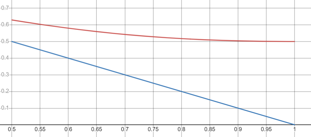
Figure 1.1. The blue curve is $1-\theta$, the red curve is $1-\theta+\ell(\theta)$

We also prove a similar result for $(n,d,\lambda)$-graphs in Theorem 4.8. In particular, our lower bound of $\alpha(G)$ improves two well-known results on the lower bound of $\alpha(G)$ of $(n,d,\lambda)$-graphs in many cases (Remark 4.10).

Let $G$ be a self-complementary graph with $n$ vertices. The Erdös-Szekeres theorem [20] implies that $\omega(G)\geq(1-o(1))\log_{4}n$. Using the recent breakthrough on diagonal Ramsey number by Campos, Griffiths, Morris, and Sahasrabudhe [9], one can deduce a better bound that $\omega(G)\geq(1-o(1))\log_{3.993}n$. In general, it is difficult to improve such a lower bound. Theorem 1.6 leads to an improved lower bound on $\omega(G)$ if $G$ has some quasi-random property. In particular, it is well-known that conference graphs form a family of quasi-random graphs with property $QR(1/2)$, and thus Theorem 1.6 implies the following corollary immediately.

Corollary 1.7.

If $X$ is a self-complementary conference graph with $n$ vertices, then $\omega(X)\geq(1-o(1))\log_{3.008}n$ as $n\to\infty$.

In the case of the graph $X_{f,q}$, the following corollary is an immediate consequence of Theorem 1.4, Theorem 1.5, and Theorem 1.6.

Corollary 1.8.

Let $d$ be a positive integer. As $q\to\infty$,

$$\frac{\omega(X_{f,q})+\alpha(X_{f,q})}{2}\geq(1-o(1))\log_{3.712}q$$

holds for all graphs $X_{f,q}\in\mathcal{X}_{d}$, and

$$\frac{\omega(X_{f,q})+\alpha(X_{f,q})}{2}\geq(1-o(1))\log_{3.008}q.$$

holds for all graphs $X_{f,q}\in\mathcal{H}_{d}$.

We also discuss an upper bound on the clique number of $X_{f,q}$ when $f$ is admissible in Corollary 3.8. When $f$ is a homogeneous admissible polynomial with an odd degree, we strengthen Corollary 1.8 as follows.

Theorem 1.9.

Let $d$ be an odd positive integer. Let $f\in{\mathbb{F}}_{q}[x,y]$ be a homogeneous admissible polynomial with degree $d$. Then $\omega(X_{f,q})\geq(1-o(1))\log_{3.712}q$ as $q\to\infty$; moreover, if $X_{f,q}\in\mathcal{H}_{d}$, then $\omega(X_{f,q})\geq(1-o(1))\log_{3.008}q$.

Both Corollary 1.7 and Theorem 1.9 imply the following corollary on Paley graphs.

Corollary 1.10.

If $q\equiv 1\pmod{4}$, then as $q\to\infty$, we have

$$\omega(P_{q})\geq(1-o(1))\log_{3.008}q.$$

Corollary 1.10 has appeared in an unpublished manuscript of Solymosi [39]. He also informed us that the same bound has been also proved in unpublished manuscripts of Alon [2], Conlon [15], and possibly others. We refer to Subsection 2.2 for other relevant results on the clique number of Paley graphs.

Lastly, we note that using the results in [9], we can obtain a slightly better bound in Theorem 1.6 that $\frac{\omega(G)+\alpha(G)}{2}\geq(1-o(1))\log_{3.705}n$ if $\theta=3/4$ and $\frac{\omega(G)+\alpha(G)}{2}\geq(1-o(1))\log_{3.003}n$ if $\theta=1/2$; see Remark 4.7. Accordingly, the other bounds of this section can be improved.

Notations. We follow standard notations in graph theory. Let us denote by $\omega(X)$ the clique number of a graph $X$, and $\alpha(X)$ the independence number of a graph $X$. We always assume $G$ is a graph with $n$ vertices. For a graph $G$, we use $\lambda_{1}(G),\lambda_{2}(G),\ldots,\lambda_{n}(G)$ to denote its eigenvalues such that $|\lambda_{1}(G)|\geq|\lambda_{2}(G)|\geq\cdots\geq|\lambda_{n}(G)|$. If there is no confusion, we denote $\lambda_{i}(G)$ by $\lambda_{i}$ for each $1\leq i\leq n$. For any vertex $v$ of $G$, we let $N(v)$ denote the neighborhood of $v$. We use the standard big $O$ notation, meaning the implicit constant is absolute, and $O_{d}$ means the implicit constant only depends on $d$. We also introduce the standard little $o$ notation.

Structure of the paper. In Section 2, we provide more background about quasi-random graphs, Paley graphs, and Diophantine tuples. In Section 3, we give some preliminary results for our proofs. In Section 4, we introduce an expander mixing lemma for quasi-random graphs and prove Theorem 1.6. In Section 5, we prove Theorem 1.4, Theorem 1.5, and Theorem 1.9.

2. More backgrounds and motivations

2.1. Known explicit constructions of quasi-random graphs

Classical examples of quasi-random graphs include cyclotomic graphs and cyclotomic sum graphs [11, 13, 30, 35, 44]. Cyclotomic sum graphs are Cayley graphs over the additive group of a finite field, with the connection set being the union of certain cosets of a fixed multiplicative subgroup. Cyclotomic sum graphs are similarly defined as Cayley sum graphs. In particular, these include Paley and Paley sum graphs. Another large family of quasi-random graphs are conference graphs (strongly regular graphs with specific parameters) [6] and many conference graphs come from finite geometry and design theory. In addition, Borbély and Sárközy [5] constructed quasi-random graphs based on circulant matrices arising from pseudo-random binary sequences, and they also recovered Paley graphs as a special case [5, Theorem 5.1]. We refer to [11, 13, 41, 43] for more explicit constructions of quasi-random graphs. It is interesting to note that the most explicit constructions of quasi-random graphs are either Cayley graphs or Cayley sum graphs, including the aforementioned explicit constructions. In particular, Cayley graphs and Cayley sum graphs are regular, and their eigenvalues can be explicitly computed via character sums, thus one can use the expander mixing lemma to verify their quasi-randomness readily.

2.2. Clique number of Paley graphs

Estimating the clique number of Paley graphs is an important open problem, due to the rich connections between Paley graphs and other problems in additive combinatorics, analytic number theory, and algebraic graph theory [16]. We refer to [47] for a discussion on the state of the art of the bounds on the clique number of Paley graphs. The trivial upper bound on $\omega(P_{q})$ is $\sqrt{q}$ [47, Lemma 1.2], and it is tight when $q$ is a square. We assume that $q$ is a non-square in the following discussion.

When $q$ is a prime, it is widely believed that $\omega(P_{q})=O_{\epsilon}(q^{\epsilon})$ for each $\epsilon>0$ (in fact, this is a special case of the more general Paley graph conjecture). However, until very recently, the trivial upper bound $\sqrt{q}$ on $\omega(P_{q})$ has been only improved to $\sqrt{q}-1$. Recently, Hanson and Petridis [25] and Yip [47] improved the $\sqrt{q}$ bound to $(1+o(1))\sqrt{q/2}$ using Stepanov’s method. Another way to obtain the same upper bound is via finite geometry [17, 45].

The best-known lower bound of $\omega(P_{q})$ is due to Cohen [14], where he showed that $\omega(P_{q})\geq(\frac{p}{p-1}-o(1))\log_{4}q$ when $q=p^{m}$ and $m\to\infty$. In particular, this implies that $\omega(P_{q})\geq(1-o(1))\log_{4}q$. Note that Cohen’s bound is strongest when $q=5^{m}$ and it gives $\omega(P_{q})\geq(1-o(1))\log_{3.032}q$ as $m\to\infty$. Thus, Corollary 1.10 always improves Cohen’s bound. On the other hand, Graham and Ringrose [21] showed that there is a constant $C>0$, such that $\omega(P_{q})\geq C\log q\log\log\log q$ holds for infinitely many primes $q\equiv 1\pmod{4}$. Moreover, under the generalized Riemann hypothesis (GRH), Montgomery [36] further improved the $C\log q\log\log\log q$ bound to $C\log q\log\log q$.

2.3. More on Diophantine tuples and Diophantine graphs

Diophantine $m$-tuples and Paley graphs are important and well-studied. They were treated completely independently, until recently Güloğlu and Murty pointed out the connection between the Paley graph conjecture and the size of Diophantine $m$-tuples in [22]. This interesting connection has been further explored in [18, 28, 29, 46]. Inspired by such a connection, we define a new graph associated with Diophantine $m$-tuples over $\mathbb{F}_{q}$, which encodes their properties.

Definition 2.1.

Let $q$ be an odd prime power. The Diophantine graph $D_{q}$ is the graph whose vertex set is $\mathbb{F}_{q}$, and two vertices $x$ and $y$ are adjacent if and only if $xy+1$ is a square in $\mathbb{F}_{q}$.

Based on the definition of Diophantine $m$-tuples over $\mathbb{F}_{q}$, we do not consider loops in $D_{q}$. Also, we note that a Diophantine tuple over ${\mathbb{F}}_{q}$ is exactly a clique in $D_{q}$. Perhaps the most important problem in the study of Diophantine tuples over ${\mathbb{F}}_{q}$ is to determine the size of the largest Diophantine tuple over ${\mathbb{F}}_{q}$, equivalently, to find the clique number $\omega(D_{q})$ of $D_{q}$. Although the above definition of Diophantine graphs appears to be new, tools from extremal graph theory and Ramsey theory have been applied to study Diophantine tuples and their generalization in several papers; see for example [7, 23, 40]. In particular, Gyarmati [23, Theorem 4] has already studied the symmetry of Diophantine graphs and proved $\omega(D_{q})\geq(1-o(1))\log_{729}q$ using three-color Ramsey numbers. We believe that obtaining a precise estimate on $\omega(D_{q})$ is of the same difficulty as estimating $\omega(P_{q})$.

Similar to the case of Paley graphs, one can verify that Diophantine graphs form a family of quasi-random graphs with property $QR(1/2)$ using Theorem 1.5. Then Theorem 1.6 implies the following corollary.

Corollary 2.2.

When $q\to\infty$, we have

$$\max\{\omega(D_{q}),\alpha(D_{q})\}\geq(1-o(1))\log_{3.008}q.$$

One may ask if we have $\omega(D_{q})\geq(1-o(1))\log_{3.008}q$. This improves the lower bound of the largest size of Diophantine tuples over ${\mathbb{F}}_{q}$. Dujella and Kazalicki [19, Theorem 17] show that the lower bound of the largest size of Diophantine tuples is $(1-o(1))\log_{4}q$. Very recently, Kim, Yip, and Yoo [29, Corollary 3.2, Theorem 3.5] improved their bound to $(\frac{p}{p-1}-o(1))\log_{4}q$ as $q=p^{m}\to\infty$, for a fixed $p$ such that $q\not\equiv 3\pmod{8}$. This is the best-known lower bound.

Using Theorem 1.6, we can also obtain the average clique number of $X_{f,q}$ when $f=axy+b$ with $a,b\in{\mathbb{F}}_{q}^{*}$. When $a=1,b=1$, this yields the case of the Diophantine graph $D_{q}$. Moreover, when $a=1$ and $b$ is nonzero, this corresponds to generalized Diophantine tuples over ${\mathbb{F}}_{q}$.

Corollary 2.3.

Let $q$ be an odd prime power. If we consider the family of graphs $X_{f,q}$ arising from the collection of polynomials $f(x,y)=axy+b$ with $a,b\in{\mathbb{F}}_{q}^{*}$, the average clique number of these graphs is at least $(1-o(1))\log_{3.008}q$ as $q\to\infty$.

Proof.

Let $r$ be a fixed non-square in ${\mathbb{F}}_{q}$. We have $\omega(X_{rf,q})\geq\alpha(X_{f,q})$ since an independent set in $X_{f,q}$ is a clique in $X_{rf,q}$. Also note that the map $f\mapsto rf$ is a bijection on $\{axy+b:a,b\in{\mathbb{F}}_{q}^{*}\}$. Thus, by Theorem 1.5 and Theorem 1.6,

$$2\sum_{a,b\in{\mathbb{F}}_{q}^{*}}\omega(X_{f,q}) =\sum_{a,b\in{\mathbb{F}}_{q}^{*}}\omega(X_{f,q})+\sum_{a,b\in{\mathbb{F}}_{q}^{*}}\omega(X_{rf,q})=\sum_{a,b\in{\mathbb{F}}_{q}^{*}}\big{(}\omega(X_{f,q})+\omega(X_{rf,q})\big{)}$$

$$\geq\sum_{a,b\in{\mathbb{F}}_{q}^{*}}\big{(}\omega(X_{f,q})+\alpha(X_{f,q})\big{)}\geq 2\sum_{a,b\in{\mathbb{F}}_{q}^{*}}(1-o(1))\log_{3.008}q.$$

It follows that the average clique number is at least $(1-o(1))\log_{3.008}q$. ∎

Furthermore, it is possible to explore more general cases. The definition of $f$-Diophantine sets was formally introduced by Bérczes, Dujella, Hajdu, Tengely [4] for a polynomial $f\in{\mathbb{Z}}[x,y]$ (see also [38]). Given a polynomial $f(x,y)\in{\mathbb{Z}}[x,y]$, a set $A\subset\mathbb{Z}$ is an $f$-Diophantine set if $f(x,y)$ is a perfect square for all $x,y\in A$ with $x\neq y$. $f$-Diophantine sets are related to many famous problems in number theory [4]. In particular, the case $f(x,y)=xy+1$ corresponds to the well-studied Diophantine tuples. Motivated by their definition, we introduce the exact analogue of $f$-Diophantine sets over finite fields. If $q$ is an odd prime power and $f=f(x,y)\in{\mathbb{F}}_{q}[x,y]$ is a polynomial, we say $A\subset\mathbb{F}_{q}$ is an $f$-Diophantine set over ${\mathbb{F}}_{q}$ if $f(x,y)$ is a square in ${\mathbb{F}}_{q}$ for all $x,y\in A$ with $x\neq y$. Note that the graph $X_{f,q}$ is naturally induced by $f$-Diophantine sets over ${\mathbb{F}}_{q}$. Similar to the study of classical Diophantine tuples, it is of special interest to give bounds on the maximum size of $f$-Diophantine sets over ${\mathbb{F}}_{q}$, or equivalently, using the graph theory language, estimate the clique number of $X_{f,q}$.

We remark that graphs arising from special multivariate polynomials over finite fields have also been explored. For example, consider the polynomial $f(\mathbf{x},\mathbf{y})=\sum_{i=1}^{n}(x_{i}-y_{i})^{2}$ that computes the square distance of two points $\mathbf{x},\mathbf{y}\in{\mathbb{F}}_{q}^{n}$. This naturally induces a graph and the clique number of this graph was studied in [27].

The quasi-randomness of Diophantine graphs has other applications in the study of Diophantine tuples over finite fields, and so do their generalizations. As an illustration, if $m$ is fixed, and $q\to\infty$, Dujella and Kazalicki [19] showed that the number of Diophantine $m$-tuples over ${\mathbb{F}}_{q}$ is $q^{m}/(2^{\binom{m}{2}}m!)+o(q^{m})$. Since Diophantine graphs are quasi-random, this also follows from the property $P_{1}(m)$ from [13]. In view of Theorem 1.4, if $d,m$ are fixed and $q\to\infty$, we have the same asymptotic for the number of $f$-Diophantine sets over ${\mathbb{F}}_{q}$ with size $m$, provided $X_{f,q}\in\mathcal{X}_{d}$.

3. Preliminaries

Throughout the section, let $f\in{\mathbb{F}}_{q}[x,y]$ be a polynomial with degree $d\geq 1$. Recall that Gyarmati and Sárközy [24, Proposition 1] showed that one can always write $f(x,y)=F(x)G(y)H(x,y)$, where $H(x,y)$ is primitive in both $x$ and $y$. Following their notations, we call $H(x,y)$ the primitive kernel of $f(x,y)$ and we note that $H(x,y)$ is unique up to a constant factor. We prove some properties of admissible polynomials and discuss their implications to graphs $X_{f,q}$. These preliminary results will be useful for the proof of our main results.

3.1. A necessary condition for $X_{f,q}$ to be Paley-like

In this subsection, we motivate the assumptions in the definitions of admissible polynomials: we show that if $X_{f,q}$ behaves like a Paley graph, then $f$ is necessarily admissible. More precisely, if the primitive kernel $H(x,y)$ is a constant multiple of a square of a polynomial, then the graph $X_{f,q}$ has a simple structure.

Lemma 3.1.

For each $a\in\overline{{\mathbb{F}}_{q}}$, $H(a,y)$ is not identically zero.

Proof.

Suppose the polynomial $H(a,y)$ is identically zero. Then $H(x,y)=H(x,y)-H(a,y)$ has the factor $x-a$. Let $k(x)$ be the minimal polynomial of $a$ over ${\mathbb{F}}_{q}$; then $k(x)$ divides $H(x,y)$ (by applying the Frobenius map $x\mapsto x^{q}$), contradicting the definition of $H$. ∎

Lemma 3.2.

Let $f\in{\mathbb{F}}_{q}[x,y]$ be with degree $d$, such that $X_{f,q}$ is an undirected graph. Let $H$ be the primitive kernel of $f(x,y)$. If $H(x,y)$ is a constant multiple of a square of a polynomial, then by removing at most $2d$ vertices and $dq$ edges from the graph $X_{f,q}$, it becomes either a complete graph, an empty graph, a complete bipartite graph, or the vertex-disjoint union of two complete subgraphs.

Proof.

We can write $f(x,y)=F(x)G(y)H(x,y)$. By scaling $F(x)$ properly, we may assume that $H(x,y)$ is a square of a polynomial.

Let $E=\{u\in{\mathbb{F}}_{q}:F(u)=0\}\cup\{v\in{\mathbb{F}}_{q}:G(v)=0\}$; it is clear that $|E|\leq 2d$. Let $Y$ be the subgraph of $X_{f,q}$, with vertex set ${\mathbb{F}}_{q}\setminus E$, such that two distinct vertices $u,v$ are adjacent if and only if $f(u,v)$ is a non-zero square in ${\mathbb{F}}_{q}$. Note that for each $u\in{\mathbb{F}}_{q}\setminus E$, the polynomial $f(u,y)$ is not identically zero by Lemma 3.1 and the assumption $F(u)\neq 0$, thus there are at most $d$ many $u\in{\mathbb{F}}_{q}$ such that $f(u,v)=0$. This shows that the graph $Y$ can be obtained from $X_{f,q}$ by removing at most $2d$ vertices and $dq$ edges.

Next, we show that $Y$ has the desired property. Let $A_{1}=\{u\in{\mathbb{F}}_{q}\setminus E:F(u)\text{ is a square in }{\mathbb{F}}_{q}\}$, and let $A_{2}={\mathbb{F}}_{q}\setminus E\setminus A_{1}$. Similarly, define $B_{1}=\{v\in{\mathbb{F}}_{q}\setminus E:G(v)\text{ is a square in }{\mathbb{F}}_{q}\}$, and let $B_{2}={\mathbb{F}}_{q}\setminus E\setminus B_{1}$. Consider the following 4 sets $A_{1}\cap B_{1}$, $A_{1}\cap B_{2}$, $A_{2}\cap B_{1}$, $A_{2}\cap B_{2}$, which form a partition of ${\mathbb{F}}_{q}\setminus E$. If both $A_{1}\cap B_{1}$ and $A_{1}\cap B_{2}$ are nonempty, then for $u\in A_{1}\cap B_{1}$ and $v\in A_{1}\cap B_{2}$, $f(u,v)=F(u)G(v)H(u,v)$ is a non-square, while $f(v,u)=F(v)G(u)H(v,u)$ is a square, violating the assumption that $f$ induces an undirected graph. Thus, either $A_{1}\cap B_{1}$ or $A_{1}\cap B_{2}$ is empty. Similarly, we can show that either $A_{1}\cap B_{1}$ or $A_{2}\cap B_{1}$ is empty, either $A_{1}\cap B_{2}$ or $A_{2}\cap B_{2}$ is empty, and either $A_{2}\cap B_{1}$ or $A_{2}\cap B_{2}$ is empty. Therefore, at most 2 of the sets of $A_{1}\cap B_{1}$, $A_{1}\cap B_{2}$, $A_{2}\cap B_{1}$, $A_{2}\cap B_{2}$ are nonempty. If there are 2 of the sets of $A_{1}\cap B_{1}$, $A_{1}\cap B_{2}$, $A_{2}\cap B_{1}$, $A_{2}\cap B_{2}$ are nonempty, then they must be either $A_{1}\cap B_{1}$ and $A_{2}\cap B_{2}$, or $A_{1}\cap B_{2}$ and $A_{2}\cap B_{1}$– in both cases, the graph $Y$ is either the vertex-disjoint union of two complete subgraphs, or a complete bipartite graph. If only one set in $A_{1}\cap B_{1}$, $A_{1}\cap B_{2}$, $A_{2}\cap B_{1}$, $A_{2}\cap B_{2}$ is nonempty, then the graph $Y$ is either a complete graph or an empty graph. ∎

3.2. Basic properties of admissible polynomials

In this subsection, we additionally assume that the primitive kernel $H$ is not a multiple of a square of a polynomial.

Lemma 3.3.

The number of $u\in{\mathbb{F}}_{q}$ such that $H(x,u)$ is a constant multiple of a square of a polynomial is at most $d^{2}+d$.

Proof.

This is implicit in the proof of [24, Theorem 5]. In [24, Lemma 4], Gyarmati and Sárközy defined the set $Y_{1}=\{u\in{\mathbb{F}}_{q}:H(x,u)=ch^{2}(x)\text{ for some }c\in{\mathbb{F}}_{q}\text{ and }h(x)\in{\mathbb{F}}_{q}[x]\}$ and proved that $|Y_{1}|\leq d^{2}+d$. ∎

Next we deduce two corollaries.

Corollary 3.4.

The number of $u\in{\mathbb{F}}_{q}$ such that $f(x,u)$ is a constant multiple of a square of a polynomial is $O(d^{2})$.

Proof.

If $f(x,u)$ is a constant multiple of a square of a polynomial, then at least one of the following happens:

• $G(u)=0$.

• $H(x,u)$ is a constant multiple of a square of a polynomial.

• $\gcd(F(x),H(x,u))$ has degree at least $1$.

The number of $u$ in the second situation is at most $d$, since the degree of $G$ is at most $d$. By Lemma 3.3, the number of $u$ in the second situation is at most $O(d^{2})$. In the third case, $F(x)$ and $H(x,u)$ have a common root $c$ in $\overline{{\mathbb{F}}_{q}}$. The common root $c$ has at most $d$ choices. Since the polynomial $H(x,c)$ is not identically zero by Lemma 3.1, the number of $u$ such that $H(x,u)=0$ is at most $d$. Thus, the number of $u$ in the third family is at most $d^{2}$. ∎

We can prove the following corollary similarly.

Corollary 3.5.

Let $C\subset{\mathbb{F}}_{q}$. The number of pairs $(u,v)\in C\times C$ such that $f(x,u)f(x,v)$ is a constant multiple of a square of a polynomial is at most $(d^{2}+d)^{2}+(d^{2}+2d)|C|$.

Proof.

Let $(u,v)\in C\times C$. If $f(x,u)f(x,v)=F(x)^{2}G(u)G(v)H(x,u)H(x,v)$ is a constant multiple of a square of a polynomial, then one of the following holds:

• $G(u)G(v)=0$.

• $H(x,u)$ and $H(x,v)$ are both a constant multiple of a square of a polynomial.

• $H(x,u)$ is not a constant multiple of a square of a polynomial, and $\gcd(H(x,u),H(x,v))$ has a degree at least $1$.

Clearly, the number of pairs $(u,v)$ in the first family is at most $2d|C|$. By Lemma 3.3, the second family has size at most $(d^{2}+d)^{2}$.

For the third family, $H(x,u),H(x,v)$ have a common root $c$ in $\overline{{\mathbb{F}}_{q}}$. Fix $u$, the common root $c$ has at most $d$ choices since $H(x,u)$ is not identically zero. We have $H(c,v)=0$. Since the polynomial $H(c,y)$ is not identically zero by Lemma 3.1, the number of $v$ such that $H(c,v)=0$ is at most $d$. Thus, the number of pairs $(u,v)$ in the third family is at most $d^{2}|C|$.

We conclude that the number of pairs $(u,v)\in C\times C$ such that $f(x,u)f(x,v)$ is a constant multiple of a square of a polynomial is at most $(d^{2}+d)^{2}+(d^{2}+2d)|C|$. ∎

3.3. Upper bound on the clique number of $X_{f,q}$

In this subsection, we derive an upper bound on $\omega(X_{f,q})$. Note that for a family $\mathcal{G}$ of quasi-random graphs with property $QR(\theta)$ and a graph $G\in\mathcal{G}$ with $n$ vertices, we have $\omega(G)=O(n^{\theta})$. Indeed, this follows from a simple observation: if $S$ is a maximum clique in $G$, then we have $e(S)=|S|(|S|-1)/2$; on the other hand, we know that $e(S)=|S|^{2}/4+O(n^{\theta}|S|)$. Theorem 1.4 thus implies that $\omega(X_{f,q})=O_{d}(q^{3/4})$, whenever $f$ is an admissible polynomial with degree $d$. However, using tools from character sums, we can show the better bound $\omega(X_{f,q})=O_{d}(\sqrt{q})$ (Corollary 3.8).

We first recall Weil’s bound for complete character sums; see for example [34, Theorem 5.41].

Lemma 3.6.

(Weil’s bound) Let $\chi$ be a multiplicative character of ${\mathbb{F}}_{q}$ of order $k>1$, and let $g\in{\mathbb{F}}_{q}[x]$ be a monic polynomial of positive degree that is not an $k$-th power of a polynomial. Let $n$ be the number of distinct roots of $g$ in its splitting field over ${\mathbb{F}}_{q}$. Then for any $a\in{\mathbb{F}}_{q}$,

$$\bigg{|}\sum_{x\in\mathbb{F}_{q}}\chi\big{(}ag(x)\big{)}\bigg{|}\leq(n-1)\sqrt{q}\,.$$

Next, we use Weil’s bound to deduce an upper bound estimate on an incomplete $2$-dimensional character sum.

Proposition 3.7.

Let $C\subset{\mathbb{F}}_{q}$. Let $f\in{\mathbb{F}}_{q}[x,y]$ be of degree $d$, such that its primitive kernel $H$ is not a multiple of a square of a polynomial. Let $\chi$ be the quadratic character. Then

$$\sum_{a,b\in C}\chi(f(a,b))=O_{d}(|C|^{3/2}q^{1/4}+|C|q^{1/2}).$$

Proof.

By Cauchy-Schwarz inequality,

$$\bigg{|}\sum_{a,b\in C}\chi(f(a,b))\bigg{|}^{2}\leq|C|\bigg{(}\sum_{a\in C}\bigg{|}\sum_{b\in C}\chi(f(a,b))\bigg{|}^{2}\bigg{)}\leq|C|\bigg{(}\sum_{x\in{\mathbb{F}}_{q}}\bigg{|}\sum_{b\in C}\chi(f(x,b))\bigg{|}^{2}\bigg{)}.$$

Note that

$$\sum_{x\in{\mathbb{F}}_{q}}\bigg{|}\sum_{b\in C}\chi(f(x,b))\bigg{|}^{2}=\sum_{u,v\in C}\bigg{(}\sum_{x\in{\mathbb{F}}_{q}}\chi(f(x,u)f(x,v))\bigg{)}.$$

If $f(x,u)f(x,v)$ is not a constant multiple of a square of a polynomial, then Weil’s bound implies the inner sum is bounded by $d\sqrt{q}.$ On the other hand, Corollary 3.5 implies that the number of pairs $(u,v)\in C\times C$ such that $f(x,u)f(x,v)$ is a constant multiple of a square of a polynomial is at most $(d^{2}+d)^{2}+(d^{2}+2d)|C|$. Therefore,

$$\sum_{u,v\in C}\bigg{|}\sum_{x\in{\mathbb{F}}_{q}}\chi(f(x,u)f(x,v))\bigg{|}\leq|C|^{2}d\sqrt{q}+((d^{2}+d)^{2}+(d^{2}+2d)|C|)q=O_{d}(|C|^{2}\sqrt{q}+|C|q).$$

We conclude that

$$\bigg{|}\sum_{a,b\in C}\chi(f(a,b))\bigg{|}^{2}=O_{d}(|C|^{3}q^{1/2}+|C|^{2}q),$$

as required. ∎

Corollary 3.8.

Let $f\in{\mathbb{F}}_{q}[x,y]$ be admissible with degree $d$. Then $\omega(X_{f,q})=O_{d}(\sqrt{q})$.

Proof.

Let $\chi$ be the quadratic character of ${\mathbb{F}}_{q}$. Let $C$ be a maximum clique of $X_{f,q}$. For each $a,b\in C$ with $a\neq b$, we have $\chi(f(a,b))=1$ unless $f(a,b)=0$. Note that if $f(x,b)$ is not identically zero, then the number of $a\in C$ such that $f(a,b)=0$ is at most $d$. On the other hand, by Corollary 3.4, the number of $b\in C$ such that $f(x,b)$ is the zero polynomial is $O(d^{2})$. It follows that

$$\sum_{a,b\in C}\chi(f(a,b))\geq\sum_{a,b\in C,a\neq b}\chi(f(a,b))-|C|\geq|C|^{2}-2|C|-d|C|-O(d^{2})|C|=|C|(|C|-O(d^{2})).$$

Combining the above lower bound estimate on $\sum_{a,b\in C}\chi(f(a,b))$ with the upper bound stated in Proposition 3.7, we conclude that $\omega(X_{f,q})=|C|=O_{d}(\sqrt{q})$. ∎

Remark 3.9.

Corollary 3.8 is best possible if $q$ is a square and $f\in{\mathbb{F}}_{\sqrt{q}}[x,y]$. Indeed, if that is the case, then the subfield ${\mathbb{F}}_{\sqrt{q}}$ forms a clique in $X_{f,q}$ since all elements in ${\mathbb{F}}_{\sqrt{q}}$ are squares in ${\mathbb{F}}_{q}$. In particular, if $q$ is a square, then $\omega(P_{q})=\sqrt{q}$.

4. quasi-random graphs

4.1. Equivalent definitions of quasi-random graphs

Let $\mathcal{G}$ be a family of graphs. In [13], Chung, Graham, and Wilson showed that the following statement, which they call $P_{3}$, is equivalent to $P_{4}$ in Definition 1.2: If for each $G\in\mathcal{G}$, we have

$$P_{3}:\quad e(G)\geq(1+o(1))\frac{n^{2}}{4},\quad\lambda_{1}=(1+o(1))\frac{n}{2},\quad\lambda_{2}=o(n)$$

as $|V(G)|=n\to\infty$. We also note that $P_{4}$ is equivalent to $P_{4}^{\prime}$ in Section 1, and we now give a short proof of this argument. It is obvious that $P_{4}^{\prime}$ implies Definition 1.2. To see the converse, note that Definition 1.2 implies that if $S,T$ are disjoint, then $e(S,T)=e(S\cup T)-e(S)-e(T)=\frac{1}{2}|S||T|+o(n^{2})$. If $S,T$ are not disjoint, let $W=S\cap T$. Hence, we have

$$e(S,T)=e(S\setminus W,T\setminus W)+2e(W)+e(S\setminus W,W)+e(T\setminus W,W)=\frac{1}{2}|S||T|+o(n^{2}).$$

Lastly, if $\mathcal{G}$ is a family of quasi-random graphs, then the following $P_{0}^{\prime}$ (proved in [13]) holds:

$$P_{0}^{\prime}:\text{ For each $G\in\mathcal{G}$, all but }o(|V(G)|)\text{ vertices of }G\text{ have degree }(1+o(1))\frac{|V(G)|}{2}.$$

4.2. No family of quasi-random graphs has property $QR(\theta)$ with $\theta<1/2$

In this subsection, we prove the following proposition.

Proposition 4.1.

There is no family of quasi-random graphs with property $QR(\theta)$, where $\theta<1/2$.

Proof.

Let $\mathcal{G}$ be a family of quasi-random graphs with property $QR(\theta)$ such that $\theta<1/2$. Let $G\in\mathcal{G}$ be a graph with $n$ vertices. Using $P_{0}^{\prime}$, we can take an induced subgraph $G^{\prime}$ with $(1-o(1))n$ vertices such that all vertices in $G^{\prime}$ have degree $(1+o(1))\frac{n}{2}$. Therefore, $\lambda_{1}(G^{\prime})=(1+o(1))\frac{n}{2}$ and

$$\lambda_{1}(G^{\prime})^{2}+\lambda_{2}(G^{\prime})^{2}+\cdots+\lambda_{|V(G^{\prime})|}(G^{\prime})^{2}=\textup{tr}((G^{\prime})^{2})=2e(G^{\prime})=\frac{1}{2}n^{2}+o(n^{2}).$$

It follows that

$$\lambda_{2}(G^{\prime})^{2}\geq\frac{\frac{1}{2}n^{2}+o(n^{2})-(1+o(1))(\frac{n}{2})^{2}}{n-1}=\frac{1}{4}n+o(n).$$

By Cauchy’s interlacing theorem, we have $|\lambda_{2}(G)|\geq(\frac{1}{2}+o(1))\sqrt{n}$. Besides, as $G\in\mathcal{G}$, we have

$$e(S,T)=\frac{|S||T|}{2}+O(n^{\theta}\sqrt{|S||T|}),$$ (4.1)

for any subsets $S,T\subset V(G)$. In particular, we have $e(G)=\frac{n^{2}}{4}+O(n^{1+\theta})$. Let $\Delta$ be the maximum degree of $G$; then trivially $\Delta\leq n$. Therefore, $\Delta/|\lambda_{2}(G)|=O(\sqrt{n})$.

On the other hand, using the partial converse to the expander mixing lemma [33, Corollary 4] due to Lev, there are non-empty subsets $S,T\subset V(G)$, such that

$$\bigg{|}e(S,T)-\frac{2e(G)}{n^{2}}|S||T|\bigg{|}\geq\frac{|\lambda_{2}(G)|}{32\sqrt{2}(\log(2\Delta/|\lambda_{2}(G)|)+4}\sqrt{|S||T|}.$$ (4.2)

Note that

$$\frac{2e(G)}{n^{2}}|S||T|=\frac{1}{2}|S||T|+O(n^{\theta-1}|S||T|)=\frac{1}{2}|S||T|+O(n^{\theta}\sqrt{|S||T|}).$$ (4.3)

It follows from 4.1, 4.2, and 4.3 that

$$O(n^{\theta}\sqrt{|S||T|})=\bigg{|}e(S,T)-\frac{1}{2}|S||T|\bigg{|}\geq\frac{|\lambda_{2}(G)|}{32\sqrt{2}(\log(2\Delta/|\lambda_{2}(G)|)+4}\sqrt{|S||T|}-O(n^{\theta}\sqrt{|S||T|}),$$

and thus

$$\frac{|\lambda_{2}(G)|}{32\sqrt{2}(\log(2\Delta/|\lambda_{2}(G)|)+4}=O(n^{\theta}),$$

which contradicts the assumption that $\theta<1/2$ since the left-hand side is $\gg\sqrt{n}/\log n$. ∎

4.3. An expander mixing lemma for quasi-random graphs

In general, it is hard to verify if a given family of graphs has property $QR(\theta)$ for a given $\theta>0$ by checking all possible subsets of vertices of graphs in the family. In this subsection, we provide a sufficient condition in terms of a quantitative version of $P_{3}$ for checking the property $QR(\theta)$. This sufficient condition can also be viewed as an expander mixing lemma for quasi-random graphs. Our proof is a refined version of the proof that $P_{3}$ implies $P_{4}$ by Chung, Graham, and Wilson [13, Theorem 1].

Lemma 4.2.

Let $\alpha<3$ and $\beta,\gamma<1$. Let $\mathcal{G}$ be a family of graphs such that the number of vertices of graphs in $\mathcal{G}$ is unbounded.

1. Assume that all graphs $G$ in the family $\mathcal{G}$ satisfy the following properties:

   $$\sum_{v\in V(G)}\Big{(}\deg(v)-\frac{n}{2}\Big{)}^{2}=O(n^{\alpha}),\quad\lambda_{1}(G)=\frac{n}{2}+O(n^{\beta}),\quad\lambda_{2}(G)=O(n^{\gamma}),$$

   where $n=|V(G)|$. Then, $\mathcal{G}$ is a family of quasi-random graphs with property $QR(\theta)$, where

   $$\theta=\max((1+\alpha)/4,\beta,\gamma).$$

2. Moreover, if each graph $G\in\mathcal{G}$ has the additional property that all but $O(1)$ vertices in $G$ have degree $n/2+O(n^{\eta})$ with $1/2\leq\eta<1$, then $\mathcal{G}$ is a family of quasi-random graphs with property $QR(\theta)$ with $\theta=\max(\eta,\beta,\gamma).$

Suppose that $\mathcal{G}$ is a family of graphs with all conditions assumed in Lemma 4.2 and let $G\in\mathcal{G}$ with $V=V(G)=\{v_{1},v_{2},\ldots,v_{n}\}$ and adjacency matrix $A$. Let $\{\bar{e}_{i}\mid i=1,2,\ldots,n\}$ denote a set of orthonormal eigenvectors corresponding to the eigenvalues $\{\lambda_{i}\mid i=1,2,\ldots,n\}$ of $A$, and set $\bar{u}=\frac{1}{\sqrt{n}}(1,1,\ldots,1)^{t}=\sum_{i}b_{i}\bar{e}_{i}$. The following claim is crucial in our proof.

Claim 4.3.

There exists a vector $\bar{z_{1}}$ such that

$$\bar{u}=(1+O(||\bar{z_{1}}||))\bar{e_{1}}+\bar{z_{1}}\quad\text{with }\quad||\bar{z_{1}}||=O(n^{\frac{\alpha-3}{4}}).$$

Moreover, under the assumption of $(2)$, we can choose $\bar{z_{1}}$ such that $||\bar{z_{1}}||=O(n^{\eta-1})$.

Proof.

For any $\epsilon>0$, we have the inequality

$$\#\{v\in V(G):\left|\deg(v)-\frac{n}{2}\right|>\epsilon n\}\leq\frac{\sum_{v}(\deg(v)-\frac{n}{2})^{2}}{\epsilon^{2}n^{2}}=\frac{O(n^{\alpha})}{\epsilon^{2}n^{2}}.$$

Thus, for any $\epsilon>0$, all but $\frac{1}{\epsilon^{2}n^{2}}O(n^{\alpha})$ vertices of $G$ have degree in $[\frac{n}{2}-\epsilon n,\frac{n}{2}+\epsilon n]$. Recall that $\bar{u}=\frac{1}{\sqrt{n}}(1,1,\ldots,1)^{t}=\sum_{i}b_{i}\bar{e_{i}}$. Then $A\bar{u}=\sum_{i}b_{i}\lambda_{i}\bar{e_{i}}$. On the other hand, the jth component of the vector $A\bar{u}$ is $\deg(v_{j})/\sqrt{n}$, where $v_{j}$ is the $j$th vertex of $G$. This implies that we can write

$$A\bar{u}=\frac{1}{2}n\bar{u}+\bar{w},$$ (4.4)

where all but $\frac{1}{\epsilon^{2}n^{2}}O(n^{\alpha})$ components of $\bar{w}$ have absolute value at most $\epsilon\sqrt{n}$. Also, note each component of $\bar{w}$ is trivially bounded above by $\frac{1}{2}\sqrt{n}$ since each component of $A\bar{u}$ is trivially in $[0,\sqrt{n}]$. It then follows that

$$||\bar{w}||^{2}\leq\frac{O(n^{\alpha})}{\epsilon^{2}n^{2}}\cdot n+n\cdot\epsilon^{2}n.$$

Now we optimize the function of $\epsilon$ on the right-hand side of the above inequality by setting $\epsilon=n^{\frac{\alpha-3}{4}}$, and thus we have

$$||\bar{w}||\leq O(n^{\frac{\alpha+1}{4}}).$$ (4.5)

Note that by equation 4.4,

$$\sum_{i=1}^{n}\left(\lambda_{i}-\frac{n}{2}\right)b_{i}\bar{e}_{i}=\bar{w}.$$

This, together with inequality 4.5, implies that

$$\left(\sum_{i=1}^{n}\left(\lambda_{i}-\frac{n}{2}\right)^{2}b_{i}^{2}\right)^{\frac{1}{2}}=||\bar{w}||\leq O(n^{\frac{\alpha+1}{4}}).$$

Since

$$\left(\sum_{i\neq 1}\left(O(n^{\gamma})-\frac{n}{2}\right)^{2}b_{i}^{2}\right)^{\frac{1}{2}}=\left|O(n^{\gamma})-\frac{n}{2}\right|\left(\sum_{i\neq 1}b_{i}^{2}\right)^{\frac{1}{2}}\leq||\bar{w}||\leq O(n^{\frac{\alpha+1}{4}}),$$

we obtain

$$\left(\sum_{i\neq 1}b_{i}^{2}\right)^{\frac{1}{2}}\leq\frac{O(n^{\frac{\alpha+1}{4}})}{\left|O(n^{\gamma})-\frac{n}{2}\right|}=O(n^{\frac{\alpha-3}{4}}).$$

Thus we have a vector $z_{1}$ such that $\bar{u}=b_{1}\bar{e}_{1}+\bar{z}_{1}$ with $||\bar{z_{1}}||\leq O(n^{\frac{\alpha-3}{4}})$. In addition, by applying the triangle inequality to $||\bar{u}||=||b_{1}\bar{e}_{1}+\bar{z}_{1}||=1$, we have $|b_{1}|=1+O(||\bar{z_{1}}||)$. By the Perron-Frobenius theorem, $b_{1}=1+O(||\bar{z_{1}}||)$, and thus $\bar{u}=(1+O(||\bar{z_{1}}||))\bar{e_{1}}+\bar{z_{1}}$, as desired.

Under the assumption of $(2)$, we have $||\bar{w}||^{2}\leq O(n^{2\eta})+O(n)=O(n^{2\eta})$. Thus $||\bar{w}||=O(n^{\eta})$, and a similar argument shows that $||\bar{z_{1}}||=O(n^{\eta-1})$. ∎

Now we are ready to prove Lemma 4.2.

Proof of Lemma 4.2.

Let $S,T\subset V$ and let $\bar{s}=(s_{1},\ldots,s_{n})$ be the characteristic vector of $S$. In other words, we have $s_{i}=1$ if $v_{i}\in S$, and $s_{i}=0$ otherwise. Let $\bar{s}^{\prime}=\bar{s}-\left\langle\bar{s},\bar{e}_{1}\right\rangle\bar{e_{1}}$. By 4.3, we have

$$\left\langle\bar{s},\bar{e}_{1}\right\rangle=\frac{|S|}{\sqrt{n}}-\left\langle\bar{s},\bar{z}_{1}+O(||\bar{z}_{1}||)\bar{e}_{1}\right\rangle=\frac{|S|}{\sqrt{n}}+O(||\bar{s}||||\bar{z_{1}}||) =\frac{|S|}{\sqrt{n}}+O(n^{\frac{\alpha-3}{4}}\sqrt{|S|}).$$ (4.6)

Similarly, let $\bar{t}=(t_{1},\ldots,t_{n})$ be the characteristic vectors of $T$, and let $\bar{t}^{\prime}=\bar{t}-\left\langle\bar{t},\bar{e}_{1}\right\rangle\bar{e_{1}}$. Note that

$$\left\langle A\bar{s}^{\prime},\bar{t}^{\prime}\right\rangle =\left\langle A\bar{s},\bar{t}\right\rangle-\left\langle\bar{s},\bar{e}_{1}\right\rangle\left\langle A\bar{e}_{1},\bar{t}\right\rangle-\left\langle\bar{t},\bar{e}_{1}\right\rangle\left\langle A\bar{s},\bar{e}_{1}\right\rangle+\left\langle\bar{s},\bar{e}_{1}\right\rangle\left\langle\bar{t},\bar{e}_{1}\right\rangle\left\langle A\bar{e}_{1},\bar{e}_{1}\right\rangle$$

$$=e(S,T)-\lambda_{1}\left\langle\bar{s},\bar{e}_{1}\right\rangle\left\langle\bar{t},\bar{e}_{1}\right\rangle.$$

Then we have

$$e(S,T)=\left\langle A\bar{s}^{\prime},\bar{t}^{\prime}\right\rangle+\lambda_{1}\left\langle\bar{s},\bar{e}_{1}\right\rangle\left\langle\bar{t},\bar{e}_{1}\right\rangle.$$

Since $\left\langle\bar{s}^{\prime},\bar{e_{1}}\right\rangle=0$ and $\left\langle\bar{t}^{\prime},\bar{e_{1}}\right\rangle=0$, it follows that

$$|\left\langle A\bar{s}^{\prime},\bar{t}^{\prime}\right\rangle|\leq|\lambda_{2}|||s^{\prime}||||t^{\prime}||\leq|\lambda_{2}|||s||||t||=O(n^{\gamma}\sqrt{|S||T|}).$$

In addition, by equation 4.6 and its analogue for $T$, we have

$$\left\langle\bar{s},\bar{e}_{1}\right\rangle\left\langle\bar{t},\bar{e}_{1}\right\rangle =\left(\frac{|S|}{\sqrt{n}}+O(n^{\frac{\alpha-3}{4}}\sqrt{|S|})\right)\left(\frac{|T|}{\sqrt{n}}+O(n^{\frac{\alpha-3}{4}}\sqrt{|T|})\right)=\frac{|S||T|}{n}+O(n^{\frac{\alpha-3}{4}}\sqrt{|S||T|}),$$

since $\alpha<3$ and $|S|,|T|\leq n$. Therefore, we deduce

$$\lambda_{1}\left\langle\bar{s},\bar{e}_{1}\right\rangle\left\langle\bar{t},\bar{e}_{1}\right\rangle =\left(\frac{n}{2}+O(n^{\beta})\right)\left\langle\bar{s},\bar{e}_{1}\right\rangle\left\langle\bar{t},\bar{e}_{1}\right\rangle=\frac{|S||T|}{2}+O(n^{\beta}\sqrt{|S||T|})+O(n^{\frac{\alpha+1}{4}}\sqrt{|S||T|})$$

since $\beta<1$ and $|S|,|T|\leq n$. We conclude that

$$e(S,T)=\left\langle A\bar{s}^{\prime},\bar{t}^{\prime}\right\rangle+\lambda_{1}\left\langle\bar{s},\bar{e}_{1}\right\rangle\left\langle\bar{t},\bar{e}_{1}\right\rangle=\frac{1}{2}|S||T|+O(n^{\theta}\sqrt{|S||T|}),$$

where $\theta=\max((1+\alpha)/4,\beta,\gamma).$

Under the assumption of $(2)$, a similar argument shows that

$$e(S,T)=\frac{1}{2}|S||T|+O(n^{\theta}\sqrt{|S||T|}),$$

where $\theta=\max(\eta,\beta,\gamma).$ ∎

Corollary 4.4.

Let $0<\alpha<2,$ and $0<\beta,\gamma<1$. Let $\mathcal{G}$ be a family of graphs such that the number of vertices of graphs in $\mathcal{G}$ is unbounded. Assume that all graphs $G$ in $\mathcal{G}$ satisfy the following properties:

$$e(G)=\frac{n^{2}}{4}+O(n^{\alpha}),\quad\lambda_{1}(G)=\frac{n}{2}+O(n^{\beta}),\quad\lambda_{2}(G)=O(n^{\gamma}),$$

where $n=|V(G)|$. Then $\mathcal{G}$ is a family of quasi-random graphs with property $QR(\theta)$, where $\theta=\theta(\alpha,\beta,\gamma)=\max((2+\alpha)/4,(3+\beta)/4,\gamma).$

Proof.

Let $G\in\mathcal{G}$ and assume that the graph $G$ has all assumed conditions. Let $A=A(G)$ be the adjacency matrix of $G$ and let $\bar{v}=(1,1,\ldots,1)^{t}$. Since $||A\bar{v}||\leq\lambda_{1}||\bar{v}||$,

$$||A\bar{v}||^{2}=\sum_{v}(\deg(v))^{2}\leq\lambda_{1}^{2}||\bar{v}||^{2}=\frac{n^{3}}{4}+O(n^{\beta+2}).$$

It follows that

$$\sum_{v}\left(\deg(v)-\frac{n}{2}\right)^{2} =\sum_{v}(\deg(v))^{2}-n\Big{(}\sum_{v}\deg(v)\Big{)}+\frac{n^{3}}{4}$$

$$\leq\frac{n^{3}}{4}+O(n^{\beta+2})-n\left(\frac{n^{2}}{2}+O(n^{\alpha})\right)+\frac{n^{3}}{4}=O(n^{\alpha+1}+n^{\beta+2}),$$

and thus the result follows immediately from Lemma 4.2. ∎

Remark 4.5.

There are several different versions of the expander mixing lemma for irregular graphs, and we refer to a recent preprint [1] and the references therein; see also [12, 32]. Among them, it appears that the version by Byrne and Tait [8] (building on the work of Krivelevich and Sudakov [32]) is closest to the classical expander mixing lemma for regular graphs. However, their version is not always good enough for our purposes, so we prove a version of the expander mixing lemma for the quasi-random graphs above.

4.4. Clique number and independence number of quasi-random graphs

In this subsection, we prove Theorem 1.6. As a preparation, we establish the following lemma using tools from Ramsey theory.

Lemma 4.6.

Let $G$ be a graph with $n$ vertices. Let $r\leq s$ be positive integers such that $n\geq\binom{r+s}{r}$. If $\omega(G)\leq r-1$, then $\omega(G)+\alpha(G)\geq r+s-1$.

Proof.

Since $r\leq s$ and $\omega(G)\leq r-1$, from the monotonicity of binomial coefficients, we have $n\geq\binom{r+s}{r}\geq\binom{r+s}{\omega(G)+1}$. By the Erdös-Szekeres theorem [20], $G$ contains an independent set of size $r+s-\omega(G)-1$. Therefore, $\alpha(G)\geq r+s-\omega(G)-1$ and thus $\omega(G)+\alpha(G)\geq r+s-1$. ∎

Proof of Theorem 1.6.

Let $G\in\mathcal{G}$. There is a constant $C>0$ (independent of $G$), such that

$$\bigg{|}e(G[S])-\frac{1}{4}|S|^{2}\bigg{|}\leq Cn^{\theta}|S|$$ (4.7)

holds for all subsets $S$ of $V(G)$. Without loss of generality, we may assume $C\geq 1$. By inequality 4.7,

$$e(G)\geq\frac{n^{2}}{4}-Cn^{\theta+1}.$$ (4.8)

We first choose a vertex $v_{1}$ with the largest degree in $G$. Then inequality 4.8 implies that

$$|N(v_{1})|\geq\frac{2e(G)}{n}\geq\frac{n}{2}-2Cn^{\theta}.$$ (4.9)

Next, we inductively choose the vertex $v_{i}$ in the induced subgraph $G_{i}=G[N(v_{1})\cap\cdots\cap N(v_{i-1})]$ with the largest degree of $G_{i}$ for each $i\geq 2$. Then, the degree of $v_{m}$ in the graph $G_{m}$ is $|N(v_{1})\cap N(v_{2})\cap\cdots\cap N(v_{m})|$, which is at least the average degree $2e(G_{m})/|V(G_{m})|$ of $G_{m}$. So, inequality 4.7 implies that

$$|N(v_{1})\cap N(v_{2})\cap\cdots\cap N(v_{m})|\geq\frac{1}{2}|N(v_{1})\cap N(v_{2})\cap\cdots\cap N(v_{m-1})|-2Cn^{\theta}$$ (4.10)

for $m\geq 2$. Then we use inequality 4.10 inductively, and this combining with inequality 4.9 gives

$$|N(v_{1})\cap N(v_{2})\cap\cdots\cap N(v_{m})| \geq\frac{1}{2^{m-1}}|N(v_{1})|-2C\Big{(}1+\frac{1}{2}+\cdots+\frac{1}{2^{m-2}}\Big{)}n^{\theta}$$

$$\geq\frac{1}{2^{m-1}}\Big{(}\frac{n}{2}-2Cn^{\theta}\Big{)}-2C\Big{(}1+\frac{1}{2}+\cdots+\frac{1}{2^{m-2}}\Big{)}n^{\theta}$$

$$\geq\frac{n}{2^{m}}-4C\Big{(}1-\Big{(}\frac{1}{2}\Big{)}^{m}\Big{)}n^{\theta}.$$ (4.11)

To obtain an lower bound of $\omega(G)$, we choose the largest $m=m(n)$ satisfying

$$\frac{n}{2^{m}}-4C\Big{(}1-\Big{(}\frac{1}{2}\Big{)}^{m}\Big{)}n^{\theta}>0,$$

equivalently,

$$\log_{2}\left(\frac{n^{1-\theta}}{4C}+1\right)>m.$$

Therefore, we have $\omega(G)\geq(1-\theta-o(1))\log_{2}n$. For the independence number, note that the complement of $G$ also satisfies inequality 4.7. Thus, the same argument shows that $\alpha(G)\geq(1-\theta-o(1))\log_{2}n$, as desired. This proves the first statement.

Next, we prove the second statement. Since the complement of $G$ also satisfies inequality 4.7, we may assume that $\omega(G)\leq\alpha(G)$ without loss of generality. Choose $m=\lfloor\log_{2}\Big{(}\frac{n^{1-\theta}}{5C}+\frac{4}{5}\Big{)}\rfloor$, so that $m=(1-\theta-o(1))\log_{2}n$. Then we have

$$2^{m}\leq\frac{n^{1-\theta}+4C}{5C}.$$ (4.12)

Then, combining inequality 4.11 with inequality 4.12 shows that

$$|N(v_{1})\cap N(v_{2})\cap\cdots\cap N(v_{m})|\geq n^{\theta}\left(\frac{n^{1-\theta}+4C}{2^{m}}-4C\right)=Cn^{\theta}\geq n^{\theta}.$$

Let $\ell=\ell(\theta)\in(0,1)$ be the unique solution to the equation

$$\theta=\ell\log_{2}\left(2+\frac{1-\theta}{\ell}\right)+(\ell+1-\theta)\log_{2}\left(1+\frac{\ell}{\ell+1-\theta}\right).$$

If $\omega(G)\geq\ell\log_{2}n+m=(1-\theta+\ell-o(1))\log_{2}n$, then we have

$$\frac{\alpha(G)+\omega(G)}{2}\geq\omega(G)\geq(1-\theta+\ell-o(1))\log_{2}n$$

and we are done. From now on, we assume that $\omega(G)<\ell\log_{2}n+m$.

We write $G^{\prime}=G[N(v_{1})\cap N(v_{2})\cap\cdots\cap N(v_{m})]$. We have shown that there are at least $n^{\theta}$ vertices in $G^{\prime}$. Set $r=\left\lfloor\ell\log_{2}n\right\rfloor$ and $s=r+m$. Next, we claim that if $n$ is sufficiently large, then

$$|V(G^{\prime})|\geq n^{\theta}\geq\binom{r+s}{s}.$$ (4.13)

Indeed, by Stirling’s formula, from the equality $\binom{r+s}{s}=\binom{2r+m}{r+m}=\frac{(2r+m)!}{r!(r+m)!}$, we deduce

$$\binom{r+s}{s} \sim\frac{(2r+m)^{2r+m+\frac{1}{2}}}{\sqrt{2\pi}r^{r+\frac{1}{2}}(r+m)^{r+m+\frac{1}{2}}}$$

$$=\frac{1}{\sqrt{2\pi r}}\left(2+\frac{m}{r}\right)^{r}\left(\frac{r}{r+m}\right)^{r+m+\frac{1}{2}}$$

$$=\frac{1}{\sqrt{2\pi\ell\log_{2}n}}\left(2+\frac{m}{\ell\log_{2}n}\right)^{\ell\log_{2}n}\left(\frac{\ell\log_{2}n}{\ell\log_{2}n+m}\right)^{\ell(\log_{2}n)+m+\frac{1}{2}}$$

It follows that if $n$ is sufficiently large, then

$$\frac{1}{\log_{2}n}\log_{2}\binom{r+s}{s}<\ell\log_{2}\left(2+\frac{1-\theta}{\ell}\right)+(\ell+1-\theta)\log_{2}\left(1+\frac{\ell}{\ell+1-\theta}\right)=\theta.$$

Therefore, if $n$ is sufficiently large, then inequality 4.13 holds, proving the claim.

Note that all vertices in $G^{\prime}$ are adjacent to the clique $\{v_{1},v_{2},\ldots,v_{m}\}$ in $G$. In particular, $\omega(G)\geq m+\omega(G^{\prime})$. Since $\omega(G)<\ell\log_{2}n+m=r+m$, we have $\omega(G^{\prime})<r$. Therefore, from inequality 4.13 and Lemma 4.6, we conclude that

$$\omega(G)+\alpha(G)\geq m+\omega(G^{\prime})+\alpha(G^{\prime})\geq m+r+s-1=2s-1=2(1-\theta+\ell-o(1))\log_{2}n,$$

as required. ∎

Remark 4.7.

Let $G\in\mathcal{G}$ with $n$ vertices. Using the recent breakthrough on Ramsey number by Campos, Griffiths, Morris, and Sahasrabudhe [9], we can further slightly improve the lower bound on $\max\{\omega(G),\alpha(G)\}$ and $(\omega(G)+\alpha(G))/2$. Using [9, Theorem 14.1], we can replace inequality 4.13 by

$$n^{\theta}\geq e^{-\frac{s}{400}+o(r)}\binom{r+s}{s}.$$

Following the same strategy of the proof of Theorem 1.6, if $\theta=1/2$, we have $\ell=0.1302$. Thus we have $\frac{\omega(G)+\alpha(G)}{2}\geq(1-o(1))\log_{3.003}n$. When $\theta=3/4$, we have $\ell=0.2792$, implying $\frac{\omega(G)+\alpha(G)}{2}\geq(1-o(1))\log_{3.705}n$.

4.5. Clique number and independence number of $(n,d,\lambda)$-graphs

Next, we turn our interest into $(n,d,\lambda)$-graphs. A graph $G$ is called an $(n,d,\lambda)$-graph if it is $d$-regular, it has $n$-vertices, and $\max_{i\geq 2}|\mu_{i}|\leq\lambda$, where $\mu_{i}$ are eigenvalues of $A(G)$ with $\mu_{1}\geq\mu_{2}\geq\ldots\geq\mu_{n}$. For $X,Y\subset V(G)$, recall the expander mixing lemma for regular graphs states that

$$\bigg{|}e(X,Y)-\frac{d}{n}|X||Y|\bigg{|}\leq\lambda\sqrt{|X||Y|}.$$

Thus, for $S\subset V(G)$, we have

$$e(G[S])\geq\frac{d}{2n}|S|^{2}-\lambda|S|.$$ (4.14)

In the following discussion, let $\theta\in(0,1)$ and let $G$ be an $(n,d,\lambda)$-graph with $\lambda=O(n^{\theta})$.

Theorem 4.8.

Let $C>0$ be a constant. Let $G$ be an $(n,d,\lambda)$-graph with $\lambda\leq Cn^{\theta}$. Then we have

$$\omega(G)\geq\log_{\frac{n}{d}}\left(\Big{(}\frac{n}{d}-1\Big{)}n^{1-\theta}\right)-\log_{\frac{n}{d}}2C,$$

$$\alpha(G)\geq\log_{\frac{n}{n-d-1}}\left(\Big{(}\frac{n}{n-d-1}-1\Big{)}n^{1-\theta}\right)-\log_{\frac{n}{n-d-1}}2C.$$

Moreover, let $k>1$ be fixed, where $k=n/d$. As $n\to\infty$, we have

$$\max\{\omega(G),\alpha(G)\}\geq(1-\theta+\ell-o(1))\log_{\frac{n}{d}}n,$$

where $\ell$ satisfies the following equation

$$\theta=\ell\log_{\frac{n}{d}}\left(2+\frac{1-\theta}{\ell}\right)+(\ell+1-\theta)\log_{\frac{n}{d}}\left(1+\frac{\ell}{\ell+1-\theta}\right).$$ (4.15)

Proof.

We follow a similar strategy as in the proof of Theorem 1.6. We first choose any vertex $v_{1}$ of $G$. Then $|N(v_{1})|=d$. Next, we inductively choose the vertex $v_{i}$ in the induced subgraph $G_{i}=G[N(v_{1})\cap\cdots\cap N(v_{i-1})]$ with the largest degree of $G_{i}$ for each $i\geq 2$. For $m\geq 2$, by setting $S=N(v_{1})\cap N(v_{2})\cap\cdots\cap N(v_{m-1})$ in inequality 4.14, it follows that

$$|N(v_{1})\cap N(v_{2})\cap\cdots\cap N(v_{m})|\geq\frac{d}{n}|N(v_{1})\cap N(v_{2})\cap\cdots\cap N(v_{m-1})|-2Cn^{\theta},$$

and this implies that

$$|N(v_{1})\cap N(v_{2})\cap\cdots\cap N(v_{m})| \geq\left(\frac{d}{n}\right)^{m-1}|N(v_{1})|-2C\Big{(}1+\frac{d}{n}+\cdots+\Big{(}\frac{d}{n}\Big{)}^{m-2}\Big{)}n^{\theta}$$

$$\geq d\Big{(}\frac{d}{n}\Big{)}^{m-1}-\frac{2Cn}{n-d}\left(1-\Big{(}\frac{d}{n}\Big{)}^{m-1}\right)n^{\theta}.$$ (4.16)

To obtain an lower bound of $\omega(G)$, we choose the largest $m=m(n)$ satisfying

$$d\Big{(}\frac{d}{n}\Big{)}^{m-1}-\frac{2Cn}{n-d}\left(1-\Big{(}\frac{d}{n}\Big{)}^{m-1}\right)n^{\theta}>0,$$

equivalently,

$$\log_{\frac{n}{d}}\left(\frac{d(n-d)}{2Cn^{\theta+1}}+1\right)+1>m.$$

Thus $\omega(G)\geq\log_{\frac{n}{d}}\left(\Big{(}\frac{n}{d}-1\Big{)}n^{1-\theta}\right)-\log_{\frac{n}{d}}2C$. Since the complement of an $(n,d,\lambda)$-graph is an $(n,n-d-1,\lambda+1)$-graph, we can do the same process to obtain a lower bound on $\alpha(G)$.

For such $m$, let $G^{\prime}=G[N(v_{1})\cap N(v_{2})\cap\cdots\cap N(v_{m})]$. Now, we want to find a clique of size $r=\lfloor\log_{\frac{n}{d}}n\rfloor$ such that

$$\theta=\ell\log_{\frac{n}{d}}\left(2+\frac{1-\theta}{\ell}\right)+(\ell+1-\theta)\log_{\frac{n}{d}}\left(1+\frac{\ell}{\ell+1-\theta}\right)$$

or an empty subgraph of size $s$ in $G^{\prime}$, which implies that $r+m\leq w(G)$ or $s\leq\alpha(G)$. Assume that $r+m=s$. Similar to the proof of Theorem 1.6, we have

$$Cn^{\theta}\geq\frac{1}{\sqrt{2\pi r}}\left(2+\frac{m}{r}\right)^{r}\left(\frac{r}{r+m}\right)^{r+m+\frac{1}{2}},$$

finishing our proof by the choice of $\ell$. ∎

Remark 4.9.

Let $k>1$ be fixed, where $k=n/d$. In Theorem 4.8, the lower bound on $\alpha(G)$ is better than $\omega(G)$ when $n$ is sufficiently large and $k>2$. Thus it is reasonable to compare the lower bound on $\alpha(G)$ with the lower bound of $\max\{\omega(G),\alpha(G)\}$. For example, let $\theta=1/2$. If $n$ is sufficiently large, we have

$$\alpha(G)\geq\left(\frac{1}{2}-o(1)\right)\log_{\frac{k}{k-1}}n\quad\text{and}\quad\max\{\alpha(G),\omega(G)\}\geq\Big{(}\frac{1}{2}+\ell-o(1)\Big{)}\log_{k}n,$$

where $\ell$ is defined in equation 4.15. This shows that the lower bound of $\max\{\alpha(G),\omega(G)\}$ is sometimes better than the lower bound of $\alpha(G)$, for example when $2\leq k<4.08$.

Remark 4.10.

We also compare our result in Theorem 4.8 with two well-known results on $\alpha(G)$ when $G$ is an $(n,d,\lambda)$-graph with $\lambda=\max\{\mu_{2},|\mu_{n}|\}$. Here, $\mu_{2}$ is the second largest eigenvalue of $G$, and $\mu_{n}$ is the smallest eigenvalue of $G$.

• Let $G$ be an $(n,d,\lambda)$-graph. Alon, Krivelevich, and Sudakov [3, Proposition 4.2] showed that if $\lambda<d\leq 0.9n$, then

  $$\alpha(G)\geq\frac{n}{2(d-\lambda)}\ln\left(\frac{d-\lambda}{\lambda+1}+1\right).$$ (4.17)

• Let $G$ be a graph with $n$ vertices, average degree $d$. Nikiforov [37, Theorem 1] showed that if $\mu_{n}(\overline{G})$ is the smallest eigenvalue of the complement graph $\overline{G}$ of $G$, and $2\leq d<n-1$, then

  $$\alpha(G)\geq\left(\frac{n}{d+1}-1\right)\left(\ln\frac{d+1}{|\mu_{n}(\overline{G})|}-\ln\ln(d+1)\right).$$ (4.18)

In [37], Nikiforov states some cases when inequality 4.18 is stronger than inequality 4.17. For example, note that Weyl’s inequalities imply $\lambda=\max\{\mu_{2}(G),|\mu_{n}(G)|\}\geq\max\{-1-\mu_{n}(\overline{G}),-1-\mu_{2}(\overline{G})\}\geq-1+|\mu_{n}(\overline{G})|$. Thus, for an $(n,d,\lambda)$-graph $G$, inequality 4.18 implies that

$$\alpha(G)\geq\left(\frac{n}{d+1}-1\right)\left(\ln\frac{d+1}{\lambda+1}-\ln\ln(d+1)\right).$$ (4.19)

Therefore, when $\lambda=o(d)$, inequality 4.19 improves inequality 4.17 by a multiplicative constant of roughly $2$ for sufficiently large $n$ and $d$.

Our bound improves inequality 4.19 in many cases. As an illustration, consider the following setting. Let $k,\theta,c,C$ be fixed real numbers such that $k>1,0<\theta<1$ and $0<c\leq C$. Let $d=n/k,cn^{\theta}\leq\lambda\leq Cn^{\theta}$, and let $n\to\infty$. Note that inequality 4.19 gives $\alpha(G)\geq(1-\theta)(k-1-o(1))\ln n$. On the other hand, Theorem 4.8 implies $\alpha(G)\geq(1-\theta-o(1))\log_{\frac{k}{k-1}}n$, which is always stronger since we have $\ln\frac{k}{k-1}<\frac{1}{k-1}$ from calculus.

5. Quasi-randomness and clique number of $X_{f,q}$

5.1. Quasi-randomness of $\mathcal{X}_{d}$

The purpose of this subsection is to show that the family $\mathcal{X}_{d}$ is a family of quasi-random graphs with property $QR(3/4)$ (Theorem 1.4). To achieve our purpose, we begin by introducing the celebrated Hoffman-Wielandt inequality for the perturbation of eigenvalues.

Lemma 5.1 (Hoffman-Wielandt inequality [26]).

Let $A,B\in M_{n,n}(\mathbb{C})$ be normal with the corresponding eigenvalues, $\lambda_{1}(A),\ldots,\lambda_{n}(A)$, and $\lambda_{1}(B),\ldots,\lambda_{n}(B)$. Then

$$\min_{\sigma\in S_{n}}\sum_{i=1}^{n}|\lambda_{i}(A)-\lambda_{\sigma(i)}(B)|^{2}\leq||A-B||^{2}.$$

Here, $S_{n}$ is the permutation group of $\{1,\ldots,n\}$, and $||A||^{2}=\sum_{1\leq i,j\leq n}|a_{i,j}|^{2}$ for any $A=(a_{i,j})\in M_{n,n}(\mathbb{C})$.

To apply Lemma 5.1, we need to estimate the entries of the square of the adjacency matrix of the graph $X_{f,q}$.

Proposition 5.2.

Let $f\in{\mathbb{F}}_{q}[x,y]$ be an admissible polynomial of degree $d$. Let $A$ be the adjacency matrix of the graph $X_{f,q}$. Then all but $O_{d}(1)$ of diagonal entries of $A^{2}$ are $q/2+O_{d}(\sqrt{q})$, and all but $O_{d}(q)$ of off-diagonal entries of $A^{2}$ are $q/4+O_{d}(\sqrt{q})$.

Proof.

We first consider the diagonal entries of $A^{2}$, which correspond to the degree of vertices in $X_{f,q}$. By Corollary 3.4, the number of $u$ such that $f(x,u)$ is a constant multiple of a square of a polynomial is $O(d^{2})$. On the other hand, if $f(x,u)$ is not a constant multiple of a square of a polynomial, then by Lemma 3.6, the degree of $u$ is

$$\frac{1}{2}\sum_{x\in{\mathbb{F}}_{q}}\Big{(}\chi(f(x,u))+\delta_{0,f(x,u)}+1\Big{)}=\frac{q}{2}+O_{d}(\sqrt{q}),$$

as required.

Next we consider off-diagonal entries of $A^{2}$. Corollary 3.4 and Corollary 3.5 imply that there are at most $O(d^{4}+d^{2}q)=O_{d}(q)$ pairs $(u,v)$ such that at least one of $f(x,u),f(x,v)$, and $f(x,u)f(x,v)$ is a constant multiple of a square of a polynomial. Thus, it suffices to show if neither $f(x,u),f(x,v)$, nor $f(x,u)f(x,v)$ is a constant multiple of a square of a polynomial, then the entry $(u,v)$ of $A^{2}$ is $q/4+O_{d}(\sqrt{q})$. Let $(u,v)$ be such a pair that neither $f(x,u),f(x,v)$, nor $f(x,u)f(x,v)$ is a constant multiple of a square of a polynomial. Let $\chi$ be the quadratic character of ${\mathbb{F}}_{q}$, and let $\eta(x)=\chi(x)+\delta_{0,x}$ so that $\eta(x)=1$ when $x$ is a square in ${\mathbb{F}}_{q}$ (including $0$), and $\eta(x)=-1$ when $x$ is a non-square in ${\mathbb{F}}_{q}$. Then the entry $(u,v)$ of $A^{2}$ can be written as

$$\frac{1}{4}\sum_{x\in\mathbb{F}_{q}}(\eta(f(x,u))+1)(\eta(f(x,v))+1)$$

$$=\frac{1}{4}\sum_{x\in\mathbb{F}_{q}}(\chi(f(x,u))+1)(\chi(f(x,v))+1)+\frac{1}{4}\sum_{x\in\mathbb{F}_{q}}\delta_{0,f(x,u)}(\chi(f(x,v))+1)$$

$$+\frac{1}{4}\sum_{x\in\mathbb{F}_{q}}\delta_{0,f(x,v)}(\chi(f(x,u))+1)+\frac{1}{4}\sum_{x\in\mathbb{F}_{q}}\delta_{0,f(x,u)}\cdot\delta_{0,f(x,v)}.$$ (5.1)

We note that

$$\frac{1}{4}\sum_{x\in\mathbb{F}_{q}}\delta_{0,f(x,u)}\cdot\delta_{0,f(x,v)}=\frac{1}{4}\#\{x\in{\mathbb{F}}_{q}~{}|~{}f(x,u)=f(x,v)=0\}=O_{d}(1),$$

$$\frac{1}{4}\sum_{x\in\mathbb{F}_{q}}\delta_{0,f(x,u)}(\chi(f(x,v))+1)=\frac{1}{4}\sum_{\begin{subarray}{c}x\in\mathbb{F}_{q}\\ f(x,u)=0\end{subarray}}(\chi(f(x,v))+1) =O_{d}(1).$$

It follows that the off-diagonal entry $(u,v)$ of $A^{2}$ is

$$\frac{q}{4}+\frac{1}{4}\sum_{x\in\mathbb{F}_{q}}\chi(f(x,u))+\frac{1}{4}\sum_{x\in\mathbb{F}_{q}}\chi(f(x,v))+\frac{1}{4}\sum_{x\in\mathbb{F}_{q}}\chi(f(x,u)f(x,v))+O_{d}(1).$$

Now Weil’s bound implies the entry $(u,v)$ is $q/4+O_{d}(\sqrt{q})$. ∎

We now have all the ingredients to show one of our main results.

Proof of Theorem 1.4.

Let $X_{f,q}\in\mathcal{X}_{d}$. Proposition 5.2 implies that all but at most $O_{d}(1)$ of vertices have degree $q/2+O_{d}(\sqrt{q})$. In particular, we have

$$\sum_{v}\Big{(}\deg(v)-\frac{q}{2}\Big{)}^{2}=O_{d}(q^{2})$$ (5.2)

and

$$e(X_{f,q})=\frac{1}{2}\sum_{u\in{\mathbb{F}}_{q}}\deg(u)=\frac{q^{2}}{4}+O_{d}(q^{3/2}).$$ (5.3)

Let $A$ be the adjacency matrix of the graph $X_{f,q}$. We approximate $A^{2}$ by $B=\frac{q}{2}I+\frac{q}{4}(J-I)=\frac{q}{4}(I+J)$, where $I$ is the identity matrix, and $J$ is the all one matrix (both $I$ and $J$ are $q\times q$ matrices). Note that the eigenvalues of $\frac{q}{4}(I+J)$ are $\frac{q}{4}$ (with multiplicity $q-1$) and $\frac{(q+1)q}{4}$ (with multiplicity $1$). By Proposition 5.2, all but at most $O_{d}(q)$ entries of $A^{2}-B$ are bounded by $O_{d}(\sqrt{q})$. Also, note that all entries of $A^{2}-B$ are trivially bounded by $q$. Let $\lambda_{i}=\lambda_{i}(X_{f,q})$. By Hoffman-Wielandt inequality, there exists $1\leq i\leq q$, such that

$$\left(\lambda_{i}^{2}-\frac{(q+1)q}{4}\right)^{2}+\sum_{1\leq j\leq q,j\neq i}\left(\lambda_{j}^{2}-\frac{q}{4}\right)^{2}\leq||A^{2}-B||^{2}\leq q^{2}O_{d}(q)+O_{d}(q)q^{2}=O_{d}(q^{3}).$$

We claim that $i=1$. Indeed, since $\lambda_{1}$ is at least the average degree of the graph $X_{f,q}$, equation 5.3 implies $\lambda_{1}\geq\frac{q}{2}+O_{d}(q^{1/2})$. If $i\neq 1$, then we would have $(\lambda_{1}^{2}-\frac{q}{4})^{2}=O_{d}(q^{3})$, which is impossible. Therefore, we have

$$\left(\lambda_{1}^{2}-\frac{(q+1)q}{4}\right)^{2}+\left(\lambda_{2}^{2}-\frac{q}{4}\right)^{2}\leq\left(\lambda_{1}^{2}-\frac{(q+1)q}{4}\right)^{2}+\sum_{j=2}^{q}\left(\lambda_{j}^{2}-\frac{q}{4}\right)^{2}\leq O_{d}(q^{3}).$$

It follows that $\lambda_{1}=\frac{q}{2}+O_{d}(q^{1/2})$ and $\lambda_{2}=O_{d}(q^{3/4})$. This, together with equation 5.2, satisfies the assumptions in Lemma 4.2. Therefore, we conclude that $\mathcal{X}_{d}$ is a family of quasi-random graphs with property $QR(3/4)$. ∎

Remark 5.3.

Note that Paley graphs are only defined over ${\mathbb{F}}_{q}$ with $q\equiv 1\pmod{4}$. Thomason [43] constructed a (undirected) Paley-like graph $G_{q}$ for a finite field ${\mathbb{F}}_{q}$ with $q=4^{n}$: the vertex set of $G_{q}$ is $PG(1,q)$, and the edge set of $G_{q}$ is defined via the trace map $\operatorname{Tr}_{{\mathbb{F}}_{q}/{\mathbb{F}}_{2}}$. He showed the graph $G_{q}$ is a self-complementary Cayley graph, $G_{q}$ is $q/2$-regular, and the co-degree of each pair is $q/4+O(\sqrt{q})$. Using these properties, he deduced that $G_{q}$ is $(1/2,q^{3/4})$-jumbled. By slightly modifying the proof of Theorem 1.4, we can show $\mathcal{G}=\{G_{q}:q=4^{n}\}$ is a family of quasi-random graphs with property $QR(3/4)$. Thus, it follows from Theorem 1.6 that $\omega(G_{q})\geq(1-o(1))\log_{3.712}q$, as $q=4^{n}\to\infty$.

5.2. Quasi-randomness of $\mathcal{H}_{d}$

In this subsection, we show that $\mathcal{H}_{d}$ is a family of quasi-random graphs with property $QR(1/2)$ (Theorem 1.5) and prove Theorem 1.9. We begin with the following lemma.

Lemma 5.4.

Let $\mathcal{G}$ be a family of graphs such that each graph in $\mathcal{G}$ is of the form $X_{f,q}$, and let $d\geq 1$. Let $\mathcal{F}_{d}$ be the family consisting of all graphs of the form $X_{h,q}$, where $g\in{\mathbb{F}}_{q}[x]$ is a polynomial with degree $d$, $h(x,y)=f(g(x),g(y))$, and $X_{f,q}\in\mathcal{G}$. If $\mathcal{G}$ is a family of quasi-random graphs with property $QR(1/2)$, then so is $\mathcal{F}_{d}$.

Proof.

Let $X_{f,q}\in\mathcal{G}$. Let $g\in{\mathbb{F}}_{q}[x]$ be a polynomial with degree $d$ and let $h(x,y)=f(g(x),g(y))$ so that $X_{h,q}\in\mathcal{F}_{d}$. We can partition ${\mathbb{F}}_{q}$ into the union of $d$ disjoint subsets $V_{1},V_{2},\ldots,V_{d}$, such that $g$ is injective on $V_{i}$ for each $1\leq i\leq d$. Now, given two subsets $S,T$ of ${\mathbb{F}}_{q}$, set $S_{i}=S\cap V_{i}$ and $T_{i}=T\cap V_{i}$. Note that if $g(u)\neq g(v)$, then the two vertices $u,v$ are adjacent in $X_{h,q}$ if and only if the two vertices $g(u),g(v)$ are adjacent in $X_{f,q}$. Note that the number of pairs of vertices $u\in S$ and $v\in T$ such that $u,v$ are adjacent in $X_{h,q}$ and $g(u)=g(v)$ is at most $d\min\{|S|,|T|\}\leq d\sqrt{|S||T|}$. Based on the above observations and the assumption that $\mathcal{G}$ is a family of quasi-random graphs with property $QR(1/2)$, in the graph $X_{h,q}$, we have

$$e(S,T) =\sum_{i,j=1}^{d}e(S_{i},T_{j})=O(d\sqrt{|S||T|})+\sum_{i,j=1}^{d}e_{X_{f,q}}(g(S_{i}),g(T_{j}))$$

$$=O(d\sqrt{|S||T|})+\sum_{i,j=1}^{d}\bigg{(}\frac{|S_{i}||T_{j}|}{2}+O(\sqrt{q|S_{i}||T_{j}|})\bigg{)}=\frac{|S||T|}{2}+O_{d}(\sqrt{q}\sqrt{|S||T|}).$$

This proves that $\mathcal{F}_{d}$ is a family of quasi-random graphs with property $QR(1/2)$, as required. ∎

Next, under some additional assumptions, we modify the proof of Theorem 1.4 to show a stronger quasi-randomness of $X_{f,q}$.

Proposition 5.5.

Let $d\geq 1$ and let $\mathcal{G}_{d}$ be an infinite subfamily of $\mathcal{X}_{d}$. Assume that for each $X_{f,q}\in\mathcal{G}_{d}$, there is a subset $B$ of ${\mathbb{F}}_{q}$ with $|B|=O(1)$, such that the entry $(u,v)$ of $A(X_{f,q})^{2}$ are $q/4+O(1)$ for all $u,v\in{\mathbb{F}}_{q}\setminus B$ with $u\neq v$. Then $\mathcal{G}_{d}$ is a family of quasi-random graphs with property $QR(1/2)$.

Proof.

Let $X_{f,q}\in\mathcal{G}_{d}$. By assumption, there exists a subset $B$ of ${\mathbb{F}}_{q}$ with $|B|=O(1)$, such that the entry $(u,v)$ of $A(X_{f,q})^{2}$ are $q/4+O(1)$ for all $u,v\in{\mathbb{F}}_{q}\setminus B$ with $u\neq v$. Let $B^{\prime}\subset{\mathbb{F}}_{q}$ be the subset of vertices of $X_{f,q}$ with degree not equal to $q/2+O_{d}(\sqrt{q})$. By Proposition 5.2, we have $|B^{\prime}|=O_{d}(1)$. Let $V^{\prime}={\mathbb{F}}_{q}\setminus B\setminus B^{\prime}$ and let $\widetilde{q}=|V^{\prime}|$; then $\widetilde{q}=q-O_{d}(1)$. Let $\widetilde{X}=\widetilde{X}_{f,q}$ be the subgraph of $X_{f,q}$ induced by $V^{\prime}$. Let $\widetilde{A}$ be the adjacency matrix of $\widetilde{X}$. Then we have

• among the diagonal entries of $\widetilde{A}^{2}$, all of them are $\widetilde{q}/2+O_{d}(\sqrt{\widetilde{q}})$;

• among the off-diagonal entries of $\widetilde{A}^{2}$, all of them are $\widetilde{q}/4+O_{d}(1)$.

Next we apply a similar argument as in the proof of Theorem 1.4 to estimate $\widetilde{\lambda_{1}}=\widetilde{\lambda_{1}}(\widetilde{X})$ and $\widetilde{\lambda_{2}}=\widetilde{\lambda_{2}}(\widetilde{X})$. Note that we have $\sum_{v\in\widetilde{X}}\Big{(}\deg(v)-\frac{\widetilde{q}}{2}\Big{)}^{2}=O_{d}(\widetilde{q}^{2})$ and $e(\widetilde{X})=\frac{\widetilde{q}^{2}}{4}+O_{d}(\widetilde{q}^{3/2})$. It follows that $\widetilde{\lambda_{1}}\geq\frac{\widetilde{q}}{2}+O_{d}(\sqrt{\widetilde{q}})$. Let us approximate $\widetilde{A}^{2}$ by $\widetilde{B}=\frac{\widetilde{q}}{2}I+\frac{\widetilde{q}}{4}(J-I)=\frac{\widetilde{q}}{4}(I+J)$, where $I$ is the identity matrix, and $J$ is the all one matrix (both $I$ and $J$ are $\widetilde{q}\times\widetilde{q}$ matrices). Note that the eigenvalues of $\frac{\widetilde{q}}{4}(I+J)$ are $\frac{\widetilde{q}}{4}$ (with multiplicity $\widetilde{q}-1$) and $\frac{(\widetilde{q}+1)\widetilde{q}}{4}$ (with multiplicity $1$). The assumptions on the entries of $\widetilde{A}^{2}$ guarantee that $||\widetilde{A}^{2}-\widetilde{B}||^{2}=O_{d}(\widetilde{q}^{2})$. Using Hoffman-Wielandt inequality, we deduce that

$$\left(\widetilde{\lambda_{1}}^{2}-\frac{(\widetilde{q}+1)\widetilde{q}}{4}\right)^{2}+\left(\widetilde{\lambda_{2}}^{2}-\frac{\widetilde{q}}{4}\right)^{2}=O_{d}(\widetilde{q}^{2})$$

and thus $\widetilde{\lambda_{1}}=\frac{\widetilde{q}}{2}+O_{d}(1)$, $\widetilde{\lambda_{2}}=O_{d}(\sqrt{\widetilde{q}})$. It then follows from Lemma 4.2 that $\widetilde{\mathcal{G}}_{d}:=\{\widetilde{X}_{f,q}:X_{f,q}\in\mathcal{G}_{d}\}$ is a family of quasi-random graphs with property $QR(1/2)$.

Now we go back to the original family $\mathcal{G}_{d}$. Note that for each $X_{f,q}\in\mathcal{G}_{d}$, the graph $\widetilde{X}_{f,q}$ is obtained from $X_{f,q}$ by deleting $O_{d}(1)$ vertices. It is straightforward to verify that $\mathcal{G}_{d}$ remains to be a family of quasi-random graphs with property $QR(1/2)$. ∎

As a corollary, the admissible polynomials of bidegree $(1,1)$ induce a family of quasi-random graphs with property $QR(1/2)$.

Corollary 5.6.

Let $\mathcal{X}_{1,1}$ be the family consisting of all graphs $X_{f,q}$ and $X_{xyf,q}$, where $f\in\mathbb{F}_{q}[x,y]$ is an admissible polynomial with bidegree $(1,1)$. Then $\mathcal{X}_{1,1}$ is a family of quasi-random graphs with property $QR(1/2)$.

Proof.

Let $f(x,y)=d+ax+by+cxy\in{\mathbb{F}}_{q}[x,y]$ be an admissible polynomial for some $a,b,c,d\in{\mathbb{F}}_{q}$. Then the coefficients satisfy $ab-cd\neq 0$. Indeed, if $d\neq 0$, then we have the factorization of the form $f(x,y)=\frac{1}{d}(ax+d)(by+d)$, violating the assumption that $f$ is admissible. If $d=0$, it is easy to verify that $f$ is not admissible.

Observe that for all but at most one $u\in{\mathbb{F}}_{q}$, the polynomial $f(x,u)\in\mathbb{F}_{q}[x]$ has degree $1$. Let $u,v\in{\mathbb{F}}_{q}$ with $u\neq v$. Then $f(x,u)f(x,v)$ has degree at most $2$, and $f(x,u)f(x,v)$ is not a constant. Suppose that the polynomial $f(x,u)f(x,v)$ is a constant multiple of a square of a polynomial, then we would have

$$f(x,u)f(x,v) =(cu+a)(cv+a)\Big{(}x+\frac{d+bu}{cu+a}\Big{)}\Big{(}x+\frac{d+bv}{cv+a}\Big{)},$$

and the constant terms of the linear factors should be the same to have a double root; this forces $\frac{d+bu}{cu+a}=\frac{d+bv}{cv+a}$, which happens only if $ab-cd=0$ as $u\neq v$, a contradiction. Let $\chi$ be the quadratic character of ${\mathbb{F}}_{q}$. Then [34, Theorem 5.48] implies

$$\bigg{|}\sum_{x\in\mathbb{F}_{q}^{*}}\chi(f(x,u)f(x,v))\bigg{|}\leq 2.$$

Hence, from equation (5.1), it is easy to verify that the off-diagonal entry $(u,v)$ of $A(X_{f,q})^{2}$ is $q/4+O(1)$, unless $f(x,u)$ or $f(x,v)$ is a constant.

Next, we consider the graph $X_{xyf,q}$. Let $u,v\in{\mathbb{F}}_{q}$ with $u\neq v$. We have

$$\sum_{x\in\mathbb{F}_{q}}\chi\big{(}xuf(x,u)\cdot xvf(x,v)\big{)}=\chi(uv)\sum_{x\in\mathbb{F}_{q}^{*}}\chi(f(x,u)f(x,v))=O(1).$$

Using a similar argument, the off-diagonal entry $(u,v)$ of $A(X_{xyf,q})^{2}$ is $q/4+O(1)$, unless $uv=0$, or one of $f(x,u)$ and $f(x,v)$ is a constant. Hence Proposition 5.5 implies the desired result. ∎

We conclude the paper with the proof of Theorem 1.5 and Theorem 1.9.

Proof of Theorem 1.5.

This follows from Lemma 5.4 and Corollary 5.6. ∎

Proof of Theorem 1.9.

Let $I$ be a maximum independent set in $X_{f,q}$ and let $r$ be a non-square in ${\mathbb{F}}_{q}$. Then $rI$ is a clique in $X_{f,q}$. Indeed, since the degree of $f$ is $d$ and $d$ is odd, $f(rx,ry)=r^{d}f(x,y)$ is a square for each $x,y\in I$. It follows that $\omega(X_{f,q})\geq\alpha(X_{f,q})$. Note that we have $\max\{\omega(X_{f,q}),\alpha(X_{f,q})\}\geq(1-o(1))\log_{3.712}q$ by Corollary 1.8. Therefore, $\omega(X_{f,q})\geq(1-o(1))\log_{3.712}q$. Similarly, if $X_{f,q}\in\mathcal{H}_{d}$, we have $\omega(X_{f,q})\geq(1-o(1))\log_{3.008}q$. ∎

References

- [1] A. Abiad and S. Zeijlemaker. A unified framework for the Expander Mixing Lemma for irregular graphs and its applications. arXiv:2401.07125, 2024.
- [2] N. Alon. On the quasirandomness of -graphs. manuscript, 2020.
- [3] N. Alon, M. Krivelevich, and B. Sudakov. List coloring of random and pseudo-random graphs. Combinatorica, 19(4):453–472, 1999.
- [4] A. Bérczes, A. Dujella, L. Hajdu, and S. Tengely. Finiteness results for -Diophantine sets. Monatsh. Math., 180(3):469–484, 2016.
- [5] J. Borbély and A. Sárközy. Quasi-random graphs, pseudo-random graphs and pseudorandom binary sequences, I. (Quasi-random graphs). Unif. Distrib. Theory, 14(2):103–126, 2019.
- [6] A. E. Brouwer and H. Van Maldeghem. Strongly regular graphs, volume 182 of Encyclopedia of Mathematics and its Applications. Cambridge University Press, Cambridge, 2022.
- [7] Y. Bugeaud and K. Gyarmati. On generalizations of a problem of Diophantus. Illinois J. Math., 48(4):1105–1115, 2004.
- [8] J. Byrne and M. Tait. Improved upper bounds on even-cycle creating Hamilton paths. arXiv:2304.02164, 2023.
- [9] M. Campos, S. Griffiths, R. Morris, and J. Sahasrabudhe. An exponential improvement for diagonal Ramsey. arXiv: 2303.09521, 2023.
- [10] F. Chung and R. Graham. Sparse quasi-random graphs. Combinatorica, 22(2):217–244, 2002.
- [11] F. R. K. Chung. Constructing random-like graphs. In Probabilistic combinatorics and its applications (San Francisco, CA, 1991), volume 44 of Proc. Sympos. Appl. Math., pages 21–55. Amer. Math. Soc., Providence, RI, 1991.
- [12] F. R. K. Chung. Spectral graph theory, volume 92 of CBMS Regional Conference Series in Mathematics. Conference Board of the Mathematical Sciences, Washington, DC; by the American Mathematical Society, Providence, RI, 1997.
- [13] F. R. K. Chung, R. L. Graham, and R. M. Wilson. Quasi-random graphs. Combinatorica, 9(4):345–362, 1989.
- [14] S. D. Cohen. Clique numbers of Paley graphs. Quaestiones Math., 11(2):225–231, 1988.
- [15] D. Conlon. A note on the Ramsey number of Paley graphs. manuscript, 2009.
- [16] E. S. Croot, III and V. F. Lev. Open problems in additive combinatorics. In Additive combinatorics, volume 43 of CRM Proc. Lecture Notes, pages 207–233. Amer. Math. Soc., Providence, RI, 2007.
- [17] D. Di Benedetto, J. Solymosi, and E. P. White. On the directions determined by a Cartesian product in an affine Galois plane. Combinatorica, 41(6):755–763, 2021.
- [18] A. B. Dixit, S. Kim, and M. R. Murty. Generalized Diophantine -tuples. Proc. Amer. Math. Soc., 150(4):1455–1465, 2022.
- [19] A. Dujella and M. Kazalicki. Diophantine -tuples in finite fields and modular forms. Res. Number Theory, 7(1):Paper No. 3, 24, 2021.
- [20] P. Erdös and G. Szekeres. A combinatorial problem in geometry. Compositio Math., 2:463–470, 1935.
- [21] S. W. Graham and C. J. Ringrose. Lower bounds for least quadratic nonresidues. In Analytic number theory (Allerton Park, IL, 1989), volume 85 of Progr. Math., pages 269–309. Birkhäuser Boston, Boston, MA, 1990.
- [22] A. M. Güloğlu and M. R. Murty. The Paley graph conjecture and Diophantine -tuples. J. Combin. Theory Ser. A, 170:105155, 9, 2020.
- [23] K. Gyarmati. On a problem of Diophantus. Acta Arith., 97(1):53–65, 2001.
- [24] K. Gyarmati and A. Sárközy. Equations in finite fields with restricted solution sets. I. Character sums. Acta Math. Hungar., 118(1-2):129–148, 2008.
- [25] B. Hanson and G. Petridis. Refined estimates concerning sumsets contained in the roots of unity. Proc. Lond. Math. Soc. (3), 122(3):353–358, 2021.
- [26] A. J. Hoffman and H. W. Wielandt. The variation of the spectrum of a normal matrix. Duke Math. J., 20:37–39, 1953.
- [27] A. Iosevich, I. E. Shparlinski, and M. Xiong. Sets with integral distances in finite fields. Trans. Amer. Math. Soc., 362(4):2189–2204, 2010.
- [28] S. Kim, C. H. Yip, and S. Yoo. Diophantine tuples and multiplicative structure of shifted multiplicative subgroups. arXiv:2309.09124, 2023.
- [29] S. Kim, C. H. Yip, and S. Yoo. Explicit constructions of Diophantine tuples over finite fields. To appear in Ramanujan J., arXiv: 2404.05514, 2024.
- [30] A. Kisielewicz and W. Peisert. Pseudo-random properties of self-complementary symmetric graphs. J. Graph Theory, 47(4):310–316, 2004.
- [31] Y. Kohayakawa, V. Rödl, M. Schacht, P. Sissokho, and J. Skokan. Turán’s theorem for pseudo-random graphs. J. Combin. Theory Ser. A, 114(4):631–657, 2007.
- [32] M. Krivelevich and B. Sudakov. Pseudo-random graphs. In More sets, graphs and numbers, volume 15 of Bolyai Soc. Math. Stud., pages 199–262. Springer, Berlin, 2006.
- [33] V. F. Lev. Discrete norms of a matrix and the converse to the expander mixing lemma. Linear Algebra Appl., 483:158–181, 2015.
- [34] R. Lidl and H. Niederreiter. Finite fields, volume 20 of Encyclopedia of Mathematics and its Applications. Cambridge University Press, Cambridge, second edition, 1997.
- [35] Q. Lin and Y. Li. Quasi-random graphs of given density and Ramsey numbers. Pure Appl. Math. Q., 18(6):2537–2549, 2022.
- [36] H. L. Montgomery. Topics in multiplicative number theory. Lecture Notes in Mathematics, Vol. 227. Springer-Verlag, Berlin-New York, 1971.
- [37] V. Nikiforov. More spectral bounds on the clique and independence numbers. J. Combin. Theory Ser. B, 99(6):819–826, 2009.
- [38] M. Sadek and N. El-Sissi. On large -Diophantine sets. Monatsh. Math., 186(4):703–710, 2018.
- [39] J. Solymosi. Clique number of Paley graphs. manuscript, 2020.
- [40] C. L. Stewart. On sets of integers whose shifted products are powers. J. Combin. Theory Ser. A, 115(4):662–673, 2008.
- [41] A. Thomason. Pseudorandom graphs. In Random graphs ’85 (Poznań, 1985), volume 144 of North-Holland Math. Stud., pages 307–331. North-Holland, Amsterdam, 1987.
- [42] A. Thomason. Random graphs, strongly regular graphs and pseudorandom graphs. In Surveys in combinatorics 1987 (New Cross, 1987), volume 123 of London Math. Soc. Lecture Note Ser., pages 173–195. Cambridge Univ. Press, Cambridge, 1987.
- [43] A. Thomason. A Paley-like graph in characteristic two. J. Comb., 7(2-3):365–374, 2016.
- [44] Q. Xiang. Cyclotomy, Gauss sums, difference sets and strongly regular Cayley graphs. In Sequences and their applications—SETA 2012, volume 7280 of Lecture Notes in Comput. Sci., pages 245–256. Springer, Heidelberg, 2012.
- [45] C. H. Yip. Exact values and improved bounds on the clique number of cyclotomic graphs. arXiv:2304.13213, 2023.
- [46] C. H. Yip. Multiplicatively reducible subsets of shifted perfect -th powers and bipartite Diophantine tuples. arXiv:2312.14450, 2023.
- [47] C. H. Yip. On the clique number of Paley graphs of prime power order. Finite Fields Appl., 77:Paper No. 101930, 2022.