Quantum entanglement and non-Gaussianity in the primordial Universe

Abstract

We propose a new method to investigate signatures of a quantum gravity phase in the primordial state of cosmological perturbations. We formulate and study a quantum model of a perturbed Friedmann-Lemaître-Robertson-Walker universe beyond the conventional Born-Oppenheimer factorization, that is, without restricting the wave function of the universe to the product of the background and perturbation wave functions. We show that the quantum dynamics generically does not preserve the product form of the universe’s wave function, that spontaneously evolves into a more general entangled state. Upon expanding this state in a suitable basis of background wave functions and setting Gaussian initial conditions for the perturbations, we numerically find that each of these wave functions becomes associated to a non-Gaussian state of an inhomogeneous perturbation.

I Introduction

The idea of quantum origin of the primordial structure in the Universe has been extensively studied for several decades. Its most prominent implementation, the theory of inflation Guth (1981); Mukhanov (2005); Peter and Uzan (2013); Martin et al. (2024a), assumes a classical background spacetime on which quantum fluctuations of the metric and matter fields propagate. However, this approach overlooks the quantum characteristics of the global geometry. It has been conjectured Borde et al. (2003) that inflationary spacetimes are past incomplete (see however Ref. Lesnefsky et al. (2023)). Consequently, various models have been developed that incorporate a quantum background geometry, potentially resolving the initial singularity and offering a dynamically complete depiction of the universe. While some of these models undergo an inflationary phase in their evolution, others serve as alternative solutions regarding the origin of the primordial Universe.

One common characteristic shared by all known quantum models is that they always rely on the Born-Oppenheimer-type dynamics (see, e.g., Peter et al. (2006); Pinho and Pinto-Neto (2007a); Ashtekar et al. (2009); Małkiewicz and Miroszewski (2021); Kiefer (2004); Bini et al. (2013); Chataignier and Krämer (2021); Kamenshchik et al. (2013); Gomar et al. (2014)). Specifically, the wave function of the universe is constrained to be the product of the wave functions for the background geometry and for each perturbation mode, with every degree of freedom maintaining a definite state at all times. This is a highly restrictive assumption as a generic quantum gravity state should exhibit some amount of entanglement. Moreover, in quantum cosmology, the universe is not in a stationary state but undergoes rapid expansion, and possibly contraction, with potentially substantial interaction between the perturbation modes and the background.

The goal of this work is to make the first step towards a more complete description of the dynamics of quantum cosmological systems. Herein, we consider a quantum bounce model of a Friedmann-Lemaître-Robertson-Walker (FLRW) universe filled with a perfect fluid and furnished with scalar perturbations. We study the dynamics of this system, setting it initially on the contracting branch in a Born-Oppenheimer (BO) state. We follow the development of this quantum state as the universe contracts, bounces and re-expands. We examine the final entangled state and identify the potential observational signatures of the quantum dynamics beyond the Born-Oppenheimer approximation.

The physical interpretation that we apply to our formalism implies the type of corrections which we obtain. In spite of the wave function being a superposition of many background states, all our observables are limited to a single branch of a semiclassical FLRW universe evolving according to the background-level Hamiltonian. We do not consider the backreaction of the perturbation on this semiclassical state, assuming it either negligible or already incorporated into the background dynamics. Rather, we focus on the effect of other backgrounds in the virtual branches of the wave function on the evolution of the perturbation itself which, as stated above, is measured only in the ‘observable’ branch. We use a quantum bounce model for this investigation so the obtained results may seem specific to the quantum bounce scenario. However, we believe that the discussed effects should be seen more broadly as coming from a quantum gravity phase of the universe and could result in a nonstandard initial condition for the inflationary models as well.

To facilitate the analysis, we restrict the Hilbert space as much as possible, allowing nevertheless for the entanglement effects to be present. We also make use of a recently discovered new class of coherent states on the half-line to conveniently represent the dynamics of the background geometry states.

The plan of this work is as follows. In Sec. II, we introduce the classical model, quantize it and use the Born-Oppenheimer basis to formulate its complete quantum dynamics. Sec. III is devoted to applying the framework to the case of two background states and their associated respective perturbation states. This simplified Hilbert space is established with the use of exact coherent states describing the background, and represents the simplest setup in which the deviations from the BO dynamics can be studied. Sec. IV presents the results of a numerical simulation while Sec. V discusses our interpretation of the results and contains some concluding remarks.

II The model

II.1 Classical Hamiltonian formalism

In this work, we study the model of scalar perturbations in a flat FLRW universe filled with a single barotropic fluid. The derivation of the physical (reduced) Hamiltonian for this model can be found, e.g., in Mukhanov et al. (1992); Pinho and Pinto-Neto (2007b); Małkiewicz (2019); Martin et al. (2022) where the physical dynamics is defined with respect to a fluid variable, denoted by $\tau$ and playing the role of internal time. For the present work, we find it more convenient to introduce another internal time, denoted by $\eta$, and corresponding to the usual conformal time. We skip here the details of this simple but tedious redefinition and only provide the final definitions of internal time, basic variables and physical Hamiltonian.

The background dynamical variables $(q,p)\in\mathbb{R}^{+}\times\mathbb{R}$ read Martin et al. (2024b)

$$\begin{split}q&=\frac{4\sqrt{6}}{(1+3w)\sqrt{1+w}}a^{(1+3w)/2}\equiv\gamma a^{(1+3w)/2},\\ p&=\frac{\sqrt{6(1+w)}}{2\kappa_{0}}a^{3(1+w)/2}H,\end{split}$$ (1)

where $H=\dot{a}/(Na)$ is the Hubble rate, $\kappa_{0}$ is a rescaled gravitational constant and $w$ is the barotropic index, i.e., the ratio of the pressure to the energy density of the fluid. We note that $p$ is a constant of motion.

In terms of the internal conformal time $\eta$, the dynamical variables $(q,p)$ form a canonical pair and the physical Hamiltonian reads

$$\begin{split}H&=H^{(0)}+\sum_{\bm{k}}H^{(2)}_{\bm{k}},\leavevmode\nobreak\ \leavevmode\nobreak\ H^{(0)}=(2\kappa_{0}){p}^{2},\\ H^{(2)}_{\bm{k}}&=\frac{1}{2}|\pi_{v,{\bm{k}}}|^{2}+\frac{1}{2}\left(wk^{2}-\mathcal{V}\right)|v_{\bm{k}}|^{2},\end{split}$$ (2)

where

$$\mathcal{V}=\frac{8(2\kappa_{0})^{2}(1-3w)}{(1+3w)^{2}}\frac{{p}^{2}}{{q}^{2}}$$

and the perturbation variable $v_{\bm{k}}$ is the usual Mukhanov-Sasaki variable. One can easily check that the above Hamiltonian generates the mode dynamics

$$v^{\prime\prime}_{\bm{k}}+\left(wk^{2}-\mathcal{V}\right)v_{\bm{k}}=0$$ (3)

for $v_{\bm{k}}$, where a prime denotes a derivative with respect to $\eta$ and $\mathcal{V}=a^{\prime\prime}/a$.

II.2 Quantization

The usual canonical prescription involves the replacements:

$$q\rightarrow\widehat{Q},\leavevmode\nobreak\ \leavevmode\nobreak\ p\rightarrow\widehat{P},$$

which in the case of compound dynamical variables $f(q,p)$ is followed by the symmetrization with respect to $\widehat{Q}$ and $\widehat{P}$. However, it turns out that the momentum operator $\widehat{P}$ defined on the half-line is not a self-adjoint operator. For this reason, we shall apply an enhanced prescription Klauder (2015) that involves the replacements:

$$q\rightarrow\widehat{Q},\leavevmode\nobreak\ \leavevmode\nobreak\ d=qp\rightarrow\widehat{D}=\frac{1}{2}(\widehat{Q}\widehat{P}+\widehat{P}\widehat{Q}),$$

which in the case of compound dynamical variables $f(q,q^{-1}d)$ is followed by the symmetrization with respect to $\widehat{Q}$ and $\widehat{D}$. Both the position $\widehat{Q}$ and dilation $\widehat{D}$ operators are self-adjoint and they generate a unitary representation of the group of affine transformations on the real line Gazeau and Murenzi (2016).

Quantization of the background Hamiltonian $H^{(0)}$ with the enhanced prescription yields

$$H^{(0)}=(2\kappa_{0})\left(\frac{d}{q}\right)^{2}\rightarrow\leavevmode\nobreak\ \widehat{H}^{(0)}=(2\kappa_{0})\left(\widehat{P}^{2}+\frac{K}{\widehat{Q}^{2}}\right),$$ (4)

where the constant $K>0$ depends on the operator ordering – see Eq. (76) of Małkiewicz et al. (2020) for more details – ; we shall assume $K>3/4$ to guarantee a unique self-adjoint realization of the above Hamiltonian. In what follows, we set $\kappa_{0}=\frac{1}{2}$.

The gravitational potential $\mathcal{V}$ of the perturbation Hamiltonian $H^{(2)}$ is then quantized through the replacement

$$\mathcal{V}\propto\frac{{d}^{2}}{{q}^{4}}\leavevmode\nobreak\ \rightarrow\leavevmode\nobreak\ \widehat{\mathcal{V}}\propto\widehat{D}\widehat{Q}^{-4}\widehat{D},$$ (5)

where a computationally convenient operator ordering has been chosen. We have checked that there exists a unique self-adjoint realization of the above quantum potential.

II.3 Background dynamics

For describing quantum states of the background, we find it useful to use a coherent state representation rather than the usual one based on self-adjoint operators such as the position (i.e., the scale factor) or the energy. We shall denote the coherent states by $|q,p\rangle$, defined with the help of a fiducial state $|\xi\rangle$ through Bergeron et al. (2024)

$$|q,p\rangle=\mathrm{e}^{-i\phi}\exp\left(\frac{ip}{2q}\hat{Q}^{2}\right)\exp\left(-i\ln q\hat{D}\right)|\xi\rangle,$$ (6)

where

$$\mathrm{e}^{-i\phi}=\left(\frac{\xi_{\nu}-iqp}{\xi_{\nu}+iqp}\right)^{\frac{\nu+1}{2}},$$

and $\nu>\frac{1}{2}$ and $\xi_{\nu}=\left[\Gamma(\nu+\frac{3}{2})/\Gamma(\nu+1)\right]^{2}$. Such states resolve the unity

$$\int|q,p\rangle\langle q,p|\leavevmode\nobreak\ \frac{\mathrm{d}q\mathrm{d}p}{2\pi c_{0}}=\mathbf{1},$$ (7)

with $c_{0}$ a normalisation factor built as an integral over the fiducial wavefunction $\xi(x)=\langle x|\xi\rangle$, explicitly

$$c_{0}=\int_{0}^{+\infty}\frac{\mathrm{d}x}{x^{2}}|\xi(x)|^{2}.$$

Such states permit to express any quantum state as a wavefunction of $(q,p)$, namely

$$|\Psi\rangle\mapsto\Psi(q,p)=\frac{\langle q,p|\Psi\rangle}{\sqrt{2\pi c_{0}}},$$ (8)

with the normalization condition $\int|\Psi(q,p)|^{2}\mathrm{d}q\mathrm{d}p=1$. Consequently, the quantity

$$\rho_{\Psi}(q,p)=|\Psi(q,p)|^{2}$$ (9)

is the phase space probability density for the state $\Psi$. For simplicity, in what follows, we assume $2\pi c_{0}\to 1$.

The coherent states themselves can serve as a kind of semi-classical states for the background geometry. The phase space probability density for a quantum state $|\tilde{\Psi}\rangle=|\tilde{q},\tilde{p}\rangle$ simply reads

$$\rho_{\tilde{q},\tilde{p}}(q,p)=|\langle q,p|\tilde{q},\tilde{p}\rangle|^{2}.$$ (10)

This formula emphasizes the fact that coherent states are not orthogonal to one another and thus form an overcomplete basis in the Hilbert space. In this work we shall use the coherent states defined on the half-line $x>0$ as

$$\langle\kern 1.29167ptx\kern 1.29167pt|\kern 1.29167ptq,p\kern 1.29167pt\rangle=\sqrt{\frac{2}{\Gamma(\nu+1)}}\left(\frac{\xi_{\nu}-iqp}{\xi_{\nu}+iqp}\right)^{\frac{\nu+1}{2}}\xi_{\nu}^{\frac{\nu+1}{2}}\,\frac{x^{\nu+1/2}}{q^{\nu+1}}\exp\left[-\frac{1}{2}(\xi_{\nu}-i\,qp)\frac{x^{2}}{q^{2}}\right].$$ (11)

It has recently been shown Bergeron et al. (2024) that within the set of coherent states defined above, there exist one-parameter families that solve the Schrödinger equation involving the Hamiltonian (4), namely

$$i\frac{\partial}{\partial\eta}|q(\eta),p(\eta)\rangle=\widehat{H}^{(0)}|q(\eta),p(\eta)\rangle,$$ (12)

where $\nu=\sqrt{K+\frac{1}{4}}$, while $q(\eta)$ and $p(\eta)$ solve the Hamilton equations derived from the semi-classical Hamiltonian

$${H}^{(0)}_{\text{sem}}=\frac{\xi_{\nu}}{\nu+1}\langle q,p|\widehat{H}^{(0)}|q,p\rangle=p^{2}+\frac{\xi_{\nu}^{2}}{q^{2}}.$$ (13)

Thus, the evolution of the variables $q(\eta)$ and $p(\eta)$ reads

$$\begin{split}q(\eta)&=q_{\textsc{b}}\sqrt{1+\left(\frac{\eta-\eta_{\textsc{b}}}{\bar{\eta}}\right)^{2}},\\ p(\eta)&=\frac{1}{2}\frac{\mathrm{d}q}{\mathrm{d}\eta}=\frac{q_{\textsc{b}}^{2}}{2\bar{\eta}q(\eta)}\left(\frac{\eta-\eta_{\textsc{b}}}{\bar{\eta}}\right),\end{split}$$ (14)

representing solutions for the scale factor according to Eq. (1). These solutions exhibit a bouncing behavior at an arbitrary time $\eta_{\textsc{b}}$ at which the scale factor reaches its minimal value $a_{\textsc{b}}=(q_{\textsc{b}}/\gamma)^{2/(1+3w)}$. Denoting by $E$ the energy $E=p^{2}(\eta)+\xi_{\nu}^{2}/q^{2}(\eta)$, constant along such a semi-classical trajectory, one obtains the other relevant parameters, namely the minimum scale as $q_{\textsc{b}}=\xi_{\nu}/\sqrt{E}$ and the typical bounce duration as $\bar{\eta}=\xi_{\nu}/E$.

II.4 Complete dynamics

In order to determine the dynamics of the full state including perturbations on top of the background, one needs to solve the Schrödinger equation

$$i\frac{\partial}{\partial\eta}|\Psi\rangle=\left(\widehat{H}^{(0)}+\widehat{H}^{(2)}\right)|\Psi\rangle,$$ (15)

where $\widehat{H}^{(2)}=\sum_{\bm{k}}\widehat{H}^{(2)}_{\bm{k}}$. The standard approach to solving this equation relies on the so-called Born-Oppenheimer approximation, which assumes the wave function to be the product of the background and the perturbation wave functions, namely $|\Psi\rangle=|\psi^{(\text{bg})}\rangle|\psi^{(\text{pert})}\rangle$. The background wave function $|\psi^{(\text{bg})}\rangle$ satisfies the background Schrödinger equation (12), while the perturbation wave function satisfies the effective perturbation Schrödinger equation:

$$i\frac{\partial}{\partial\eta}|\psi^{(\text{pert})}\rangle=\langle\psi^{(\text{bg})}|\widehat{H}^{(2)}|\psi^{(\text{bg})}\rangle\,|\psi^{(\text{pert})}\rangle,$$ (16)

where the quantum gravitational potential $\widehat{\mathcal{V}}$ is replaced by the quantum average $\langle\psi^{(\text{bg})}|\widehat{\mathcal{V}}|\psi^{(\text{bg})}\rangle$, or another $c-$number that includes a quantum correction.

The standard approach thus neglects the entanglement between the background and perturbation wave functions. However, starting with a simple product state, the entanglement must eventually be produced by gravitational dynamics which couples perturbations to the background. Therefore, starting as

$$|\Psi\rangle=|\psi^{(\text{bg})}_{0}\rangle|\psi^{(\text{pert})}_{0}\rangle,$$

the quantum state after some time is expected to read

$$|\Psi(\eta)\rangle=\sum_{n}|\psi_{n}^{(\text{bg})}(\eta)\rangle|\psi_{n}^{(\text{pert})}(\eta)\rangle,$$ (17)

with a nonvanishing state vector $|\psi_{n}^{(\text{bg})}(\eta)\rangle|\psi_{n}^{(\text{pert})}(\eta)\rangle$ for some $n>0$ Małkiewicz and Miroszewski (2021). The background states $|\psi_{n}^{(\text{bg})}(\eta)\rangle$ ($n=0,1,\dots$) can be assumed to solve the background Schrödinger equation and form a (time-dependent) basis in the background Hilbert space. The dynamics of the perturbation states $|\psi_{n}^{(\text{pert})}(\eta)\rangle$ is nontrivial and can in principle depend on other perturbation states $|\psi_{m}^{(\text{pert})}(\eta)\rangle$ with $m\neq n$.

Upon substituting the general state (17) into the full Schrödinger equation (15) we find

$$i\frac{\partial}{\partial\eta}|\psi_{n}^{(\text{pert})}\rangle=\sum_{\ell m}M_{n\ell}^{-1}\widehat{H}^{(2)}_{\ell m}|\psi_{m}^{(\text{pert})}\rangle,$$ (18)

where $\widehat{H}^{(2)}_{\ell m}=\langle\psi_{\ell}^{(\text{bg})}|\widehat{H}^{(2)}|\psi_{m}^{(\text{bg})}\rangle$ is a matrix representation of $\widehat{H}^{(2)}$ in the background Hilbert space and $M_{nm}=\langle\psi_{n}^{(\text{bg})}|\psi_{m}^{(\text{bg})}\rangle$ is the matrix of scalar products between the background solutions. We clearly see that assuming initially $|\psi_{0}^{(\text{pert})}(\eta)\rangle\neq 0$, the dynamics generically produces non-trivial $|\psi_{n}^{(\text{pert})}(\eta)\rangle$ for $n>0$ as long as $\langle\psi_{n}^{(\text{bg})}|\widehat{H}^{(2)}|\psi_{0}^{(\text{bg})}\rangle\neq 0$. Hence, the background universe starting out from a simple ‘semiclassical’ state $|\psi_{0}^{(\text{bg})}(\eta)\rangle$ eventually evolves into a multi-branched state (17).

We conclude that a quantum multiverse naturally emerges in this approach even though no “third quantization" Caderni and Martellini (1984) is performed on the gravitational field. However natural the presence of the multiverse may appear from the point of view of ordinary quantum mechanics, it poses a severe interpretational problem in quantum cosmology and complicates taking the classical limit in which the observable universe must be recovered. The viewpoint which we adopt in this work is that the fixed background solution $|\psi_{0}^{(\text{bg})}(\eta)\rangle$ and its associated perturbation state $|\psi_{0}^{(\text{pert})}(\eta)\rangle$ underlie our classical universe with its inhomogeneous perturbation in the sense that at late times the latter provides a reasonable approximation to (or, realization of) the quantum solution $|\psi_{0}^{(\text{bg})}(\eta)\rangle|\psi_{0}^{(\text{pert})}(\eta)\rangle$. All other background solutions $|\psi_{n}^{(\text{bg})}(\eta)\rangle$ for $n>0$ are “virtual" with their only role to generate an interaction loop $|\psi_{0}^{(\text{pert})}(\eta)\rangle\leftrightarrow|\psi_{n}^{(\text{pert})}(\eta)\rangle$ in the dynamics of the “observed" perturbation $|\psi_{0}^{(\text{pert})}(\eta)\rangle$ belonging to the physical background universe $|\psi_{0}^{(\text{bg})}(\eta)\rangle$, according to the dynamical law (18).

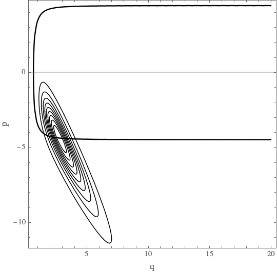
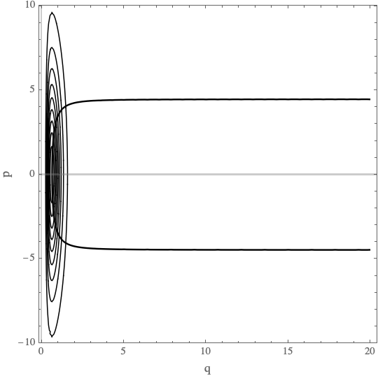
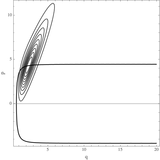
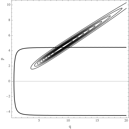
Figure 1: The bouncing evolution of the probability distribution (from top left to bottom right) of a coherent state (11) for $\nu=2$, $E=20$ and $\eta=-0.3,0,0.25,1$.

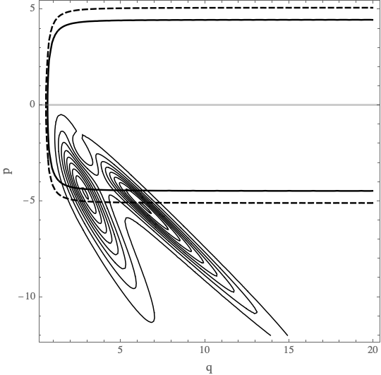
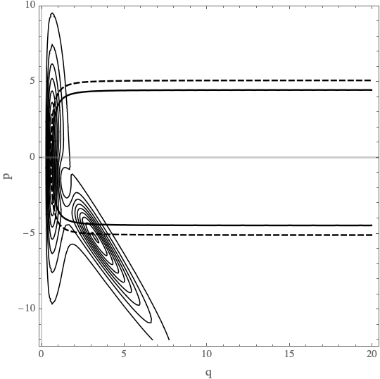
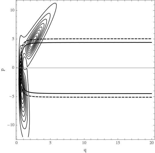
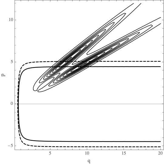
Figure 2: The evolution of the probability distribution (from top left to bottom right) of a combination of two coherent states (11) with the energies and the bouncing times respectively $E=20,26$ and $\eta_{b}=0,0.3$, for $\nu=2$ and $\eta=-0.3,0,0.25,1$.

Before concluding this section let us reformulate the general dynamics (18) in terms of a fixed basis in the perturbation Hilbert space. We assume a basis in the perturbation Hilbert space such that the parameter labelling the basis’ elements belongs to the same parameter space as in the case of the background Hilbert space. We denote the basis’ elements by $\{|\phi_{m}\rangle\}$,

$$|\psi_{n}^{(\text{pert})}\rangle=\sum_{m}\alpha_{nm}|\phi_{m}\rangle,$$ (19)

for all $n$. Furthermore, we assume the basis’ elements to evolve according to the Born-Oppenheimer dynamical law with the background solution sharing the same label $n$, that is,

$$i\partial_{\eta}|\phi_{n}\rangle=\langle\psi_{n}^{(\text{bg})}|\widehat{H}^{(2)}|\psi_{n}^{(\text{bg})}\rangle|\phi_{n}\rangle.$$ (20)

The entire dynamics is encoded in the complex parameters $\alpha_{nm}$ that satisfy the following dynamical law:

$$\begin{split}i{\alpha}_{nm}^{\prime}=\sum_{\ell rkp}M_{n\ell}^{-1}S_{mk}^{-1}{H}^{(2)}_{\ell rkp}\alpha_{rp}-\sum_{kp}S_{mk}^{-1}{H}^{(2)}_{ppkp}\alpha_{np},\end{split}$$ (21)

where ${H}^{(2)}_{\ell mkp}=\langle\phi_{k}|\widehat{H}^{(2)}_{\ell m}|\phi_{p}\rangle$ is a complete matrix representation of the operator $\widehat{H}^{(2)}$ and $S_{kp}=\langle\phi_{k}|\phi_{p}\rangle$ is the matrix of scalar products between the perturbation solutions. The matrices $\widehat{H}^{(2)}_{\ell m}$ and $M_{n\ell}$ are defined below Eq. (18).

Our goal for the next section is to study a specific example and verify if the condition $\langle\psi_{0}^{(\text{bg})}|\widehat{H}^{(2)}|\psi_{n}^{(\text{bg})}\rangle\neq 0$ for $n>0$ can indeed hold and lead to substantial modification of the Born-Oppenheimer dynamics (16).

III Biverse

In what follows, we study only a single mode of perturbation $\bm{k}$, and restrict the cosmological setup to two independent background solutions $|\psi_{0}^{(\text{bg})}(\eta)\rangle=|q_{0}(\eta),p_{0}(\eta)\rangle$ and $|\psi_{1}^{(\text{bg})}(\eta)\rangle=|q_{1}(\eta),p_{1}(\eta)\rangle$, with respective energies $E_{0}$ and $E_{1}$. We use the respective perturbation solutions to the Born-Oppenheimer dynamics (16), denoted here by $|\phi_{E_{0}}(\eta)\rangle$ and $|\phi_{E_{1}}(\eta)\rangle$, to form a two-dimensional basis for the perturbation states, namely $|\psi_{0}^{(\text{pert})}(\eta)\rangle=\alpha_{00}(\eta)|\phi_{E_{0}}(\eta)\rangle+\alpha_{01}(\eta)|\phi_{E_{1}}(\eta)\rangle$ and $|\psi_{1}^{(\text{pert})}(\eta)\rangle=\alpha_{10}(\eta)|\phi_{E_{0}}(\eta)\rangle+\alpha_{11}(\eta)|\phi_{E_{1}}(\eta)\rangle$, where $|\phi_{E_{0}}(\eta)\rangle$ and $|\phi_{E_{1}}(\eta)\rangle$ are fixed by Eq. (20), which reads in this case

$$\begin{split}i\partial_{\eta}|\phi_{E_{0}}\rangle&=\langle q_{0}(\eta),p_{0}(\eta)|\widehat{H}^{(2)}_{\bm{k}}|q_{0}(\eta),p_{0}(\eta)\rangle|\phi_{E_{0}}\rangle,\\ i\partial_{\eta}|\phi_{E_{1}}\rangle&=\langle q_{1}(\eta),p_{1}(\eta)|\widehat{H}^{(2)}_{\bm{k}}|q_{1}(\eta),p_{1}(\eta)\rangle|\phi_{E_{1}}\rangle,\end{split}$$ (22)

with the asymptotic vacuum state set as the initial state. The complete state thus reads

$$\begin{split}|\Psi(\eta)\rangle&=|q_{0},p_{0}\rangle\left[\alpha_{00}(\eta)|\phi_{E_{0}}(\eta)\rangle+\alpha_{01}(\eta)|\phi_{E_{1}}(\eta)\rangle\right]\\ &+|q_{1},p_{1}\rangle\left[\alpha_{10}(\eta)|\phi_{E_{0}}(\eta)\rangle+\alpha_{11}(\eta)|\phi_{E_{1}}(\eta)\rangle\right].\end{split}$$ (23)

The dynamical law (21) is then applied to the state (23) in order to derive the dynamics for the amplitudes $\alpha_{00}$, $\alpha_{01}$, $\alpha_{10}$ and $\alpha_{11}$.

Working in the Schrödinger representation with $H^{(2)}_{\bm{k}}$ defined in (2), we find, with $i,j\in\{0,1\}$,

$$\begin{split}\hat{H}_{ij}^{(2)}=\left(-\frac{1}{2}\frac{\partial^{2}}{\partial v_{\bm{k}}^{2}}+\frac{1}{2}wk^{2}v_{\bm{k}}^{2}\right)M_{ij}-\frac{1}{2}\mathcal{V}_{ij}v_{\bm{k}}^{2},\end{split}$$ (24)

where $\mathcal{V}_{ij}=\langle q_{i},p_{i}|\widehat{\mathcal{V}}|q_{j},p_{j}\rangle$ and

$$M_{ij}:=\langle q_{i},p_{i}|q_{j},p_{j}\rangle=\int\mathrm{d}x\langle q_{i},p_{i}|x\rangle\langle x|q_{j},p_{j}\rangle,$$

whose integration leads, through the explicit form (11), to

$$M_{ij}=\left[\frac{2\left(\displaystyle\frac{\xi_{\nu}+ip_{i}q_{i}}{\xi_{\nu}-ip_{i}q_{i}}\right)^{1/2}\left(\displaystyle\frac{\xi_{\nu}-ip_{j}q_{j}}{\xi_{\nu}+ip_{j}q_{j}}\right)^{1/2}}{\left(\displaystyle\frac{q_{j}}{q_{i}}+\frac{q_{i}}{q_{j}}\right)+\displaystyle\frac{i}{\xi_{\nu}}\left(p_{i}q_{j}-p_{j}q_{i}\right)}\right]^{\nu+1}.$$ (25)

It is also possible to obtain the potential $\mathcal{V}_{ij}$ analytically. Using Eq. (6) and the commutation relation $[\hat{Q},\hat{D}]=i\hat{Q}$, one finds

$$\hat{D}e^{i\phi}|q,p\rangle=i\left(q\frac{\partial}{\partial q}-p\frac{\partial}{\partial p}\right)e^{i\phi}|q,p\rangle,$$

which permits to calculate $\hat{D}|q,p\rangle$ and subsequently the necessary matrix elements for the potential $\langle q_{i},p_{i}|\hat{D}\hat{Q}^{-4}\hat{D}|q_{j},p_{j}\rangle$ through

$$\langle q_{i},p_{i}|\hat{D}\hat{Q}^{-4}\hat{D}|q_{j},p_{j}\rangle=e^{i(\phi_{i}-\phi_{j})}\left(q_{i}\frac{\partial}{\partial q_{i}}-p_{i}\frac{\partial}{\partial p_{i}}\right)\left(q_{j}\frac{\partial}{\partial q_{j}}-p_{j}\frac{\partial}{\partial p_{j}}\right)e^{i(\phi_{j}-\phi_{i})}\langle q_{i},p_{i}|\hat{Q}^{-4}|q_{j},p_{j}\rangle.$$

Using the representation (11), this leads to the Hermitian matrix

$$\begin{split}\mathcal{V}_{ij}=\frac{2(1-3w)}{(1+3w)^{2}\nu(\nu-1)}\left\{(\nu+1)(\nu-3)\left[\frac{p_{i}^{2}}{q_{i}^{2}}+\frac{p_{j}^{2}}{q_{j}^{2}}+2i\xi_{\nu}\left(\frac{p_{i}}{q_{i}^{3}}-\frac{p_{j}}{q_{j}^{3}}\right)-\xi_{\nu}^{2}\left(\frac{1}{q_{i}^{4}}+\frac{1}{q_{j}^{4}}\right)\right]\right.\\ \left.+(\nu^{2}+3)\left[2\frac{p_{i}}{q_{i}}\frac{p_{j}}{q_{j}}-2i\xi_{\nu}\left(\frac{p_{i}}{q_{i}q_{j}^{2}}-\frac{p_{j}}{q_{j}q_{i}^{2}}\right)+\frac{\xi_{\nu}^{2}}{q_{i}^{2}q_{i}^{2}}\right]\right\}M_{ij},\end{split}$$ (26)

which, for $i=j$, reduces to

$$\mathcal{V}_{ii}=\frac{8(1-3w)}{(1+3w)^{2}}\left[\frac{p_{i}^{2}}{q^{2}_{i}}+\frac{\nu+3}{\nu(\nu-1)}\frac{\xi_{\nu}^{2}}{q_{i}^{4}}\right].$$ (27)

Furthermore, assuming the following Gaussian perturbation representation

$$\langle v_{\bm{k}}|\phi_{E_{i}}\rangle=\left[\frac{2\Re\mathrm{e}(\Omega_{i})}{\pi}\right]^{1/4}\exp\left[-\Omega_{i}(\eta)v_{\bm{k}}^{2}\right],$$ (28)

it is straightforward to calculate the matrix elements ${H}_{ijkl}^{(2)}$. One obtains

$$\begin{split}H_{ijkl}^{(2)}=\sqrt{2}M_{ij}\left[\Re\mathrm{e}\left(\Omega_{k}\right)\Re\mathrm{e}\left(\Omega_{l}\right)\right]^{\frac{1}{4}}\left[\frac{\Omega_{l}}{(\bar{\Omega}_{k}+\Omega_{l})^{\frac{1}{2}}}-\frac{\Omega_{l}^{2}}{(\bar{\Omega}_{k}+\Omega_{l})^{\frac{3}{2}}}+\frac{wk^{2}-\mathcal{V}_{ij}/M_{ij}}{4(\bar{\Omega}_{k}+\Omega_{l})^{\frac{3}{2}}}\right].\end{split}$$ (29)

The Born-Oppenheimer equations (22) can be rewritten in terms of the mode functions $f_{i}(\eta)$ that satisfy the mode equation

$$\begin{split}f^{\prime\prime}_{i}+(wk^{2}-\mathcal{V}_{ii})f_{i}=0.\end{split}$$ (30)

This mode function permits to recover the variance through

$$\Omega_{i}=-\frac{i}{2}\frac{f^{\prime}_{i}}{f_{i}},$$ (31)

and therefore to reconstruct the perturbation wave function (28).

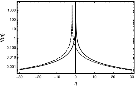
Figure 3: The evolution of the potentials $V_{00}(\eta)$ (full line) and $V_{11}(\eta)$ (dashed line) appearing in the mode equations (34). For illustrative purposes, in this figure and the following ones, we assume $w\to\frac{1}{6}$ for definiteness. The potentials are seen to act mostly at the bounce location for both bounces.

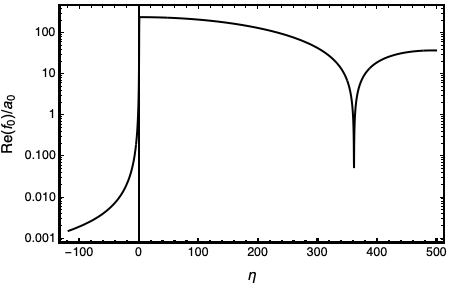
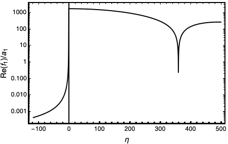
Figure 4: The evolution of $\Re\mathrm{e}(f_{0})/a_{0}$ and $\Re\mathrm{e}(f_{1})/a_{1}$ for $k=0.01$. The first perturbation gets amplified around the first background bounce at $\eta=0$, whereas the second one around the second background bounce at $\eta=-2$. The second background is more massive than the first one ($E_{1}>E_{0}$) and thus the second amplitude gets more amplified than the first, i.e., $\Re\mathrm{e}(f_{1})/a_{1}>\Re\mathrm{e}(f_{0})/a_{0}$.

IV Results

The coherent states (11) represent a bouncing universe. In what follows, we use the family of time-independent coherent states $(q,p)\mapsto|q,p\rangle$ to give a probabilistic interpretation to the quantum state of the universe and its evolution. The relevant formula is given in the Appendix. As can be seen from Fig. 1, the probability distribution (for a fixed $E$) that is obtained reads

$$\rho_{E}(q,p,\eta)=|\psi_{E}(q,p,\eta)|^{2}=\left|\int_{0}^{\infty}\mathrm{d}x\langle q,p|x\rangle\langle x|\psi_{E}\rangle\right|^{2},$$ (32)

with $\psi_{E}(q,p,\eta)$ defined as in Eq. (8), namely its "$x$" representation is given by Eq. (11) with $q\mapsto q(\eta)$ and $p\mapsto p(\eta)$ from Eq. (14) corresponding to the value $E$ for the energy.

The density (32) first approaches the singular boundary $q=0$ with $p<0$ (contraction), then bounces against the boundary (big bounce) and finally moves away from the boundary with $p>0$ (expansion). The distribution exhibits a simple shape and a simple dynamics that is symmetric with respect to the bounce. The background trajectory is obtained from the expectation values of $\widehat{Q}$ and $\widehat{P}$, denoted respectively as $q$ and $p$. As pointed out in Subsec. II.3, the background trajectories solve the dynamics implied by the semiclassical Hamiltonian and are given by Eq. (14).

Suppose that the background wave function spreads into a combination of two coherent states with different energies and bouncing times. Then the probability distribution for such a ‘biverse’ is a more complicated function of $q$, $p$ and $\eta$. In Fig. 2 we plot a probability distribution for a biverse with equal weights for each component universe:

$$\rho_{E_{0},E_{1}}(q,p,\eta)=\frac{|\psi_{E_{0}}(q,p,\eta-\eta_{0})+\psi_{E_{1}}(q,p,\eta-\eta_{1})|^{2}}{2(1+\Re\mathrm{e}\langle q_{0},p_{0}|q_{1},p_{1}\rangle)}.$$ (33)

The dynamics is no longer symmetric with respect to the bounce that happens at different times for different components. Interference between these two components is noticeable. Each component follows its semiclassical trajectory.

We now turn to the main numerical computation of the paper: a case of two Born-Oppenheimer universes. In the following we assume the numerical values $\nu=2$, $E_{0}=10$, $E_{1}=80$, $\eta_{0}=0$, $\eta_{1}=-2$, and $k=0.01$. We determine the perturbation wave function on each component universe $\langle v_{\bm{k}}|q_{0},p_{0}\rangle$ and $\langle v_{\bm{k}}|q_{1},p_{1}\rangle$ by solving the mode equations for $f_{0}(\eta)$ and $f_{1}(\eta)$, namely

$$\begin{split}f^{\prime\prime}_{0}+\left(wk^{2}-\langle q_{0},p_{0}|\widehat{\mathcal{V}}|q_{0},p_{0}\rangle\right)f_{0}=0,\\ f^{\prime\prime}_{1}+\left(wk^{2}-\langle q_{1},p_{1}|\widehat{\mathcal{V}}|q_{1},p_{1}\rangle\right)f_{1}=0,\end{split}$$ (34)

with the initial condition corresponding to the asymptotic vacuum state: $f_{i}(-\infty)=(2\sqrt{w}k)^{-1/2}$ and $f^{\prime}_{i}(-\infty)=i\sqrt{\sqrt{w}k/2}$. The potentials $V_{00}(\eta)=\langle q_{0},p_{0}|\widehat{\mathcal{V}}|q_{0},p_{0}\rangle$ and $V_{11}(\eta)=\langle q_{1},p_{1}|\widehat{\mathcal{V}}|q_{1},p_{1}\rangle$ are plotted in Fig. 3.

The behavior of the mode functions $f_{0}$ and $f_{1}$ for $k=0.01$ is plotted in Fig. 4. The maximum amplification of the amplitudes $\Re\mathrm{e}(f_{0})$ and $\Re\mathrm{e}(f_{1})$ occurs respectively at $\eta\approx-2$ and $\eta\approx 0$, which is consistent with the corresponding bounce times. In the second, more massive background the amplitude amplification is stronger. These solutions form a basis in which we shall express the perturbation wave function (23) determined by the fuller dynamical law (21).

The background wave functions $|q_{0},p_{0}\rangle$ and $|q_{1},p_{1}\rangle$ are not orthogonal as their overlap (which is constant in time) is of order of $10^{-4}$. This fact is incorporated in the dynamics (18) by the matrix element $M_{01}$. However, the key quantity in the process of entangling the two component universes is their overlap on the potential $V_{01}(\eta)=\langle q_{0},p_{0}|\hat{\mathcal{V}}|q_{1},p_{1}\rangle$ that is plotted in Fig. 5. Its value is largest at the bounces.

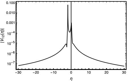
Figure 5: The evolution of the overlap $\langle\psi_{E_{0}}|\hat{\mathcal{V}}|\psi_{E_{1}}\rangle$ between the two component universes on the gravitational potential. This quantity is responsible for the interaction between the universes with their primordial structures.

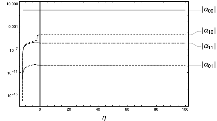
Figure 6: The evolution of $|\alpha_{00}|$, $|\alpha_{01}|$, $|\alpha_{10}|$ and $|\alpha_{11}|$. The value of $|\alpha_{00}|$ hardly changes as the produced probability amplitude for the other universe $\alpha_{11}$ as well as the entanglement amplitudes $\alpha_{01}$, $\alpha_{10}$ are very small. The numerical violation of unitarity is kept under control.

We assume the ansatz (23) and set $\alpha_{00}=1$, $\alpha_{01}=0$, $\alpha_{10}=0$ and $\alpha_{11}=0$ initially. Thus, initially there is no virtual universe $|q_{1},p_{1}\rangle$ and the perturbations on $|q_{0},p_{0}\rangle$ are expected to satisfy the Born-Oppenheimer dynamics. As expected from the dynamics (21), such an initial solution is unstable and the other universe with its internal perturbation immediately emerges and influences the structure formation on the observable branch $|q_{0},p_{0}\rangle$. As a result we obtain the dynamics of $\alpha_{00}$, $\alpha_{01}$, $\alpha_{10}$ and $\alpha_{11}$ as plotted in Fig. 6.

As can be seen in this figure, the amplitude $\alpha_{00}$ is only very mildly modified, while the other $\alpha_{ij}$ are only slighly increased, with a hierarchy of values. This is a consequence of our chosen set of parameter values, and a full study over the parameter space and for many different wavelengths should be performed to evaluate its genericness.

Fig. 7 illustrates the changes observed in the initial perturbation states within both backgrounds when their interaction is considered. The probability distribution of the primordial amplitude is much more concentrated in the observed background compared to the virtual one, indicating a larger amplification of amplitude in the latter. As a result of the full dynamics, the probability distribution of the perturbation amplitude in the first background exhibits a long tail at larger values of $v$, however, with relatively insignificant total probability. On the other hand, the distribution of the second perturbation becomes significantly altered, noticeably shifting towards the smaller values of $v$. These probability distributions evolve over time, and the plots represent a fixed moment of time at $\eta=25$. The new distributions exhibit visibly non-Gaussian characteristics, although symmetric (no skewness).

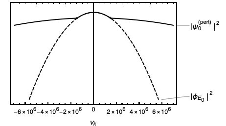
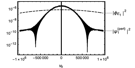
Figure 7: The probability distributions for the perturbation amplitude at $\eta=25$ when the perturbations are superhorizon and constant. Top: The Born-Oppenheimer perturbation state on the background ‘0’ evolves into a combination with a small but discernible contribution from the Born-Oppenheimer perturbation state originating from the background ‘1’. This contribution can be seen in the final distribution at very large amplitudes $v_{\bm{k}}$. Bottom: For background ‘1’, the initial perturbation is eventually overcome by a dominant contribution from the perturbation associated with the background ‘0’, leading to a significant shift in the probability distribution towards smaller values of $v_{\bm{k}}$.

V Discussion

We have developed a framework which fully captures the influence of the cosmological background on the linear perturbations. Choosing conveniently the Born-Oppenheimer universes for basis vectors in the state space, and truncating the model to four degrees of freedom, we have found that the expanding universe generically emerges in an entangled state. Upon projecting it onto an observable background, the primordial perturbation becomes well-defined but exhibits non-Gaussian behavior. However, the degree of non-Gaussianity appears to be very small in the numerical example presented herein. An analogous numerical computation (not shown in the paper) shows that reversing the roles of the two BO universes in the initial condition yields a similarly inverted final state.

While the amount of non-Gaussianity in our example is extremely small for the observable branch, it is premature to assert that the Born-Oppenheimer approximation will invariably yield such accurate results. The current study represents merely a proof of concept, i.e., the first step towards understanding the dynamics beyond the Born-Oppenheimer approximation. A more comprehensive numerical investigation should be constructed based on an analytical definition of the BO universes. This approach would enable to manipulate parameters within the truncated model, such as the energies of backgrounds and the times of their bounces, to determine the situations in which calculating corrections to a Born-Oppenheimer universe is most useful.

Moreover, we should include perturbation modes of other wavelengths in our analysis. Their presence may dramatically change the dynamical picture obtained thus far. Specifically, these modes could combine to exert a stronger influence on the backgrounds as well as become entangled with one another, yielding non-negligible effects on the expanding universe. Enhancing the method presented here by identifying the optimal basis or proposing an entirely different, more efficient approach could greatly help to derive new and important physical results.