Optimal crawling: from mechanical to chemical actuation

Abstract

Taking inspiration from the crawling motion of biological cells on a substrate, we consider a physical model of self-propulsion where the spatio-temporal driving can involve both, a mechanical actuation by active force couples, and a chemical actuation through controlled mass turnover. We show that the competition and cooperation between these two modalities of active driving can drastically broaden the performance repertoire of the crawler. When the material turnover is slow and the mechanical driving dominates, we find that the highest velocity at a given energetic cost is reached when actuation takes the form of an active force configuration propagating as a traveling wave. As the rate of material turnover increases, and the chemical driving starts to dominate the mechanical one, such a peristalsis-type control progressively loses its efficacy, yielding to a standing wave type driving which involves an interplay between the mechanical and chemical actuation. Our analysis suggests a new paradigm for the optimal design of crawling biomimetic robots where the conventional purely mechanical driving through distributed force actuators is complemented by a distributed chemical control of the material remodeling inside the force-transmitting machinery.

I Introduction

In living systems the crawling mode of motility is ubiquitous and its thorough understanding on both mechanical and biochemical levels constitutes an important fundamental challenge [1, 2, 3, 4]. The parallel problem of the design of soft robots that can efficiently crawl by themselves is an equally important engineering problem [5, 6, 7, 8, 9, 10] which have been mostly studied from the perspective of a purely mechanical driving in the form of distributed actuators generating “active” force couples [11, 12, 13, 14, 15, 16, 17, 18]. In this paper, taking inspiration from the importance of chemical processes in the crawling motion of biological objects, we consider the situation where in addition to a mechanical actuation, the crawler material can turnover through a process driven by an out of equilibrium chemical reaction.

There exists two fundamentally different paradigms to represent the overdamped crawling motion of an active object on a solid substrate. One of them, which builds on older swimming theories [19, 20, 21], assumes that the shape of a deformable object is dynamically actuated to harvest friction forces with its environment. The motion is supported by the breaking of the time reversal symmetry of each periodic stroke [22]. As initially formulated by Purcell in the context of swimming at a low Reynolds number, this necessary condition to obtain a net motion over a stroke is known as the scallop Theorem [23, 24, 25]. The optimality of such motion as a function of the actuation can be quantified by the Stokes efficiency which compares how much energy is dissipated during each stroke with the power to move the crawler center of mass at a certain velocity against the frictional background [26, 27, 28, 29]. Limbless animals such as millipedes, caterpillars or earthworms are good natural representatives of this category of crawlers.

The development of active gel theories allowing one to model the motility of various types of biological cells [30] has paved the way for an alternative paradigm where the crawler is constituted of a mechanical skeleton (scaffold) which can chemically turnover through its polymerization and de-polymerization. The fundamental point here is that while the skeleton is in frictional contact with the external environment, its de-polymerized building blocks are not, in the same manner as the lower part of the belt of a rolling tank-tread transmits tractions to the ground while the upper part of the belt does not. The mechanical actuation of the skeleton by distributed contractile forces then creates a steady state flow [31]. The spatial analogue of the scallop Theorem would then state that to ensure self propulsion the flow of skeleton must be asymmetric with respect to the crawler center. As a result, the friction forces on the background will also lose their symmetry, leading to directional motion [32, 33]. However, the fact that the skeleton is being permanently advected in a particular direction requires to “close the stroke”. This means that there must be sources and sinks allowing material renewal and depletion, where necessary through an implicit chemical reaction [34]. Again, the Stokes efficiency for such type of motion has been introduced and the corresponding optimal regimes were identified [35]. While the implied modeling approach is most simply formulated in the context of an object crawling on a stiff substrate, it was also shown to be fully capable of explaining various regimes of swimming in a liquid [36].

The goal of the present paper is to bring together these two paradigms within a single simple prototypical framework. Specifically, we consider a 1D soft elastic body with free boundaries, where material can be chemically driven to undergo internal mass redistribution and, in addition, can be mechanically driven through a distributed field of active stresses. Such system may then be actuated both mechanically and chemically. It can be seen as representing in a very simplified way the propulsion machinery of a cell. It would be then implied that the active mechanical stress is controlled by a distribution of internally driven molecular motors cross-linking skeleton filaments, while the active mass redistribution is governed by a chemical potential representing an internal out of equilibrium chemical reservoir of monomers that can be polymerized into filament form. In this respect, it is worth mentioning, that the chemical pathways regulating both the cytoskeleton contractility and its turnover can now be externally controlled with light in both space and time using two different optogenetics constructions [37, 38].

One of our main results is the realization that the interplay between the chemical and mechanical modalities of active controls crucially depends on the relative rate of the corresponding kinetic processes. Thus, we show that slow turnover can hinder the chemical control while large viscosity can obstruct the work of molecular motors. We characterize the relative importance of chemical versus mechanical activity by a single dimensionless parameter $\lambda$, and study its role in the choice of the optimal crawling gait. More precisely, we ask how the optimal actuation strategy adjusts as $\lambda$ increases from zero to infinity and whether one can identify transitions between different crawling gaits initiated by the variation of $\lambda$.

In particular, we show that in order to ensure optimal efficacy, our two modalities of external driving, mechanical and chemical, must cooperate. In other words, the two controlling agents must conspire if the goal is to achieve the best performance at a fixed total metabolic cost. How the corresponding mechanical and biochemical pathways are organized to reach the necessary level of coherency is beyond the scope of this work where we neglect the chemo-mechanical feedbacks between the active agents and the dynamical variables representing, for instance, the flow or the density of material.

To formulate the optimal control problem we assume that our driving mechanisms arrive with an energetic cost. We show how the latter can be specified based on some basic thermodynamic arguments. We then use a simple close-to-equilibrium Onsager formalism to introduce the corresponding kinetic processes. This allows us to specify the two time scales characterizing the mechanical and chemical drivings and formally define the parameter $\lambda$ as ratio of these time scales.

As the most basic assumption, we associate the performance of the propulsion with the average velocity of the crawler and solve in two limiting cases the mathematical optimization problem delivering the best actuation strategy at a fixed energetic cost. In agreement with previous investigations [39, 14, 40], we find that in the case of slow material turnover, the most effective time periodic actuation strategy is a traveling wave propagating along the body. In the opposite limit, when turnover is fast and both mechanical and chemical actuators are relevant, the optimal driving is represented by a standing wave. In the latter case, the combined chemo-mechanical actuation and the associated cooperation between chemistry and mechanics in driving the internal dynamics, allows the system to reach a higher performance than in the absence of turnover at the same energetic cost.

Using a simple ansatz linking the two limiting cases, when either mechanics or chemistry dominates, we study the crossover between the traveling wave type and the standing wave type modalities of crawling as the parameter $\lambda$ varies continuously. We show that the implied crossover is accompanied by a switch in the allocation of the energetic resources from the purely mechanical driving towards an optimal balance between mechanical and chemical energy inputs. More specifically, we show that as the rate of material turnover increases, and the chemical driving starts to dominate the mechanical one, the commonly accepted peristalsis-type control progressively loses its efficacy, yielding to a standing wave type driving which now involves a constructive interplay between the mechanical and chemical actuation.

In addition to offering new insights regarding the different fundamental modalities of the functioning of living matter, our analysis can be viewed as providing a new paradigm for the design of soft robots that crawl on rigid surfaces. The main novelty is in the replacement of the conventional purely mechanical driving through distributed force actuators, by a chemo-mechanical driving involving the possibility to chemically activate or dis-activate the dynamic renewal of the internal force-transmitting scaffold.

The paper is organized as follows. In Sec. II we derive a thermodynamically consistent chemo-mechanical model of a driven one dimensional crawling segment with free boundaries. In Sec. III, we introduce the main non-dimensional parameter. The time periodic chemo-mechanical actuation fields that control the dynamics are introduced in Sec. IV. In Sec. V, based on the energy balance discussed in Sec. II, we formulate the optimization problem whose solution allows one to specify the optimal chemo-mechanical control. We then study two limitings cases where the optimal actuation protocol can be found explicitly. Specifically, in Sec. VII we assume that material turnover is slow compared to mechanical relaxation while in Sec. VIII we consider the opposite limit. Finally, we introduce in Sec. IX an ansatz for the actuation fields that interpolates the two above limits. It enables us to study the interplay between the chemical and mechanical actuation when the relative rate of turnover varies continuously and identify a transition between the two major gaits of chemo-mechanical crawling. Our conclusions are summarized in Sec. X.

II The model

We consider a prototypical model of a bio-mimetic object crawling along a one-dimensional track on a rigid substrate. The skeleton of this one dimensional crawler is effectively represented as a continuum segment with material points indexed by the actual spatial coordinate $x\in[l_{-}(t),l_{+}(t)]$. Here the two moving boundaries representing the front and rear edges of the crawler are $l_{-}(t)$ and $l_{+}(t)$ with $t\geq 0$ denoting the time. The deformed state of the system is described by the time dependent functions $x(X,t)$, where by $X$ we denote the reference positions of the actual points.

In view of the anticipated role of the chemically-driven mass turnover of the skeleton, we describe the mechanical response of the system using the framework of morpho-elasticity [41, 42]. We start by introducing the deformation gradient $F(x,t)=\partial x/\partial X$ and decompose $F$ multiplicatively into

$$F=AG.$$

Here $A(x,t)$ is the 1D analog of the elastic distortion which can be considered in this setting as purely volumetric. We suppose that such a distortion is counted from an unstressed configuration with a fixed density $\rho_{m}$. Then the actual (current) density of the material is $\rho(x,t)=\rho_{m}/A(x,t)$. The scalar function $G(x,t)$ describes the stress free swelling due to the arrival or departure of the material “building blocks” needed to assemble the configuration with the density $\rho_{m}$. Such configuration can then be interpreted as intermediate because the primordial configuration of the “building blocks” would be characterized by another density $\rho_{0}(x,t)=G(x,t)\rho_{m}$. The function $G(x,t)$ is a 1D analog of the growth tensor in morpho-elasticity describing the swelling of the material from density $\rho_{0}(x,t)$ to the density $\rho_{m}$ while the scalar $A$ is the deformation gradient necessary to accommodate such a swelling into the actual stressed configuration. The thermodynamical configuration of the resulting material capable of both, elastic deformation and inelastic renewal, is described by two mechanical (dynamic) variables which may be either $A(x,t)$ and $G(x,t)$ or $\rho(x,t)$ and $\rho_{0}(x,t)$.

Mass balance. In the Eulerian coordinate system, the equation of mass balance can be rewritten in the form

$$\partial_{t}\rho+\partial_{x}(\rho v)=r,$$ (1)

where

$$d/dt=\partial_{t}+v\partial_{x},$$

$v=\partial_{t}x(X,t)$ is the velocity of material points, and the mass supply is

$$r=\rho\left(\frac{1}{G}\frac{dG}{dt}\right),$$

see e.g. [43]. It is clear from (1) that it is the temporal variation of $G$ which brings the local sources/sinks of mass. For instance, in the context of living cell, this term represents the polymerization and depolymerization of the cytoskeleton filaments which is controlled by a monomers reservoir [44]. As we do not consider any flux of mass through the boundaries, we shall also assume that

$$\dot{l}_{\pm}=v(l_{\pm}(t),t).$$

Momentum balance. Since inertia is negligible in our setting, we can write force balance in the form

$$\partial_{x}\sigma=f_{f},$$ (2)

where $\sigma(x,t)$ is the axial stress and $f_{f}$ is the bulk force describing the interaction of the skeleton with the rigid substrate in a thin film limit. We further assume that

$$\sigma(x,t)=\sigma_{e}(x,t)+\sigma_{a}(x,t),$$ (3)

where $\sigma_{e}(x,t)$ is the elastic stress and $\sigma_{a}(x,t)$ is an active stress, representing the mechanical driving and effectively describing the momentum exchange with an out of equilibrium reservoir. One can also think directly in terms of the driving bulk force and the elastic restoring force:

$$f_{a}(x,t)=\partial_{x}\sigma_{a}\text{ and }f_{e}=-\partial_{x}\sigma_{e}.$$

The former can be exogenous (say, originating from external actuators such as an applied magnetic field affecting embedded beads) or endogenous (say, describing myosin molecular motors cross-linking actin filaments). The boundary condition associated with (2) is

$$\sigma(l_{-}(t),t)=\sigma(l_{+}(t),t),$$

which implies the existence of a stiff spring representing a constraint which connects the two edges of the crawling system $l_{+},l_{-}$ and ensures that its total length

$$L=l_{+}(t)-l_{-}(t)$$

remains constant.

Energy balance. We consider that the system is isothermal and introduce its free energy in the form

$$\Psi=\int_{l_{-}}^{l_{+}}\rho\psi(A,G)\mathrm{d}x,$$ (4)

where we assume that elasticity and turnover are uncoupled material properties of the skeleton:

$$\psi(A,G)=\psi_{e}(A)+\psi_{c}(G).$$

For simplicity, we consider as variable only the mechanical contribution $\psi_{e}(A)$ while the chemical contribution $\psi_{c}(G)=\tilde{\psi}$ is assumed constant. This reflects the fact that only variations of the elastic strain change the stored internal energy while the amount of stress-free swelling due to material turnover does not impact the chemical free energy as it is often formulated in classical morpho-elastic theories [45]. In view of the local mass conservation (1) we obtain:

$$\frac{d\Psi}{dt}=\int_{l_{-}}^{l_{+}}\left(r\psi+\rho\frac{d\psi}{dt}\right)\mathrm{d}x=\int_{l_{-}}^{l_{+}}(\sigma_{e}\partial_{x}v+r\mu_{c})\mathrm{d}x,$$

where we introduced the elastic stress in the skeleton

$$\sigma_{e}=\rho_{m}\frac{\partial\psi_{e}}{\partial A},$$

and the chemical potential of the skeleton

$$\mu_{c}=\psi-A\frac{\partial\psi_{e}}{\partial A}.$$

Next we need to introduce the exerted power $\Pi$. Since we assumed for simplicity that there are no boundary traction forces (no cargo to carry), such a power is delivered only in the bulk, through both active stresses and active mass exchange. The power of active forces acting on the system has the standard form of mechanical work per unit time

$$\Pi^{m}=\int_{l_{-}}^{l_{+}}f_{a}v\mathrm{d}x.$$

Similarly, the power of generalized forces performing regulation of mass exchange and acting at the chemical level, can be written as

$$\Pi^{c}=\int_{l_{-}}^{l_{+}}\mu_{a}r\mathrm{d}x.$$

The external mass reservoir is characterized by the chemical potential $\mu_{a}(x,t)$ which is a direct chemical analog of $f_{a}(x,t)$, while the rate of the exchange reaction $r(x,t)$ is the analog of the local velocity $v(x,t)$.

Due to the fact that our system is active, the integral energy inequality representing the second law of thermodynamics can be interpreted in two equivalent forms.

First, considering $f_{a}$ and $\mu_{a}$ as internal drivings, we can write the integral energy balance as $-d\Psi/dt=\hat{R}$ where the function $\hat{R}=R-(\Pi^{m}+\Pi^{c})$ describes all energy exchanges due to the interaction between the material system described by the energy (4) and the machinery operating to maintain the active terms. The latter includes the rate of supply of mechanical and chemical energy due to microscopic active agents $\Pi^{m}+\Pi^{c}$ and the irreversible dissipation $R\geq 0$ characterizing the interaction of the system with a thermal reservoir. Note that if the active agents are designed to always operate in the regime where $\Pi^{m}+\Pi^{c}\geq 0$, as will be the case in the rest of the paper, the corresponding entry in $\hat{R}$ can be considered as representing “anti-dissipation”.

The second approach, which we effectively use in what follows, is based on the assumption that the power $\Pi^{m}+\Pi^{c}$ represents an external work. We can then write the integral energy balance in the form

$$R =\Pi^{m}+\Pi^{c}-\frac{d\Psi}{dt}$$ (5)

$$=\int_{l_{-}}^{l_{+}}\left[(f_{a}-f_{e})v+\left(\mu_{a}-\mu_{c}\right)r\right].$$

Here the dissipation

$$R\geq 0,$$

is interpreted as the difference between the work done per unit time by the macroscopic active agents $\Pi^{m}+\Pi^{c}$ and the concurrent rate of change of the macroscopic free energy of the system $d\Psi/dt$, see e.g. [35, 46].

To ensure that the term $R$ representing the dissipated energy, is non-negative as required by the second law of thermodynamics, we make the simplest assumption that the linear Onsager close-to-equilibrium theory [47] is operative. Specifically, we assume that the thermodynamic fluxes and forces are linearly related so that

$$\begin{array}[]{lcl}f_{a}-f_{e}=\xi v\\ \mu_{a}-\mu_{c}=\nu r.\end{array}$$ (6)

In (6), we have neglected chemo-mechanical cross terms and introduced the purely mechanical friction coefficient $\xi>0$ and the purely chemical kinetic coefficient $\nu>0$. Under these assumptions, friction with the substrate, mimicking interaction with the mechanical reservoir, and kinetic turnover of the material, mimicking interaction with the chemical reservoir, represent two sources of quadratic dissipation in the system. As we show below, the two parameters, $\xi$ and $\nu$, set the timescales of the corresponding mechanical and chemical relaxation processes and their dimensionless ratio is an important control parameter of the problem.

Specification of the model. We further impose for simplicity that the free energy represents only entropic elasticity and set

$$\psi_{e}(A)=\psi_{0}(A\log(A)-A),$$ (7)

where $\psi_{0}$ characterizes the elastic stiffness of the material. The chosen expression (7) can be viewed as reflecting a skeleton containing almost ideal polymer chains. Note that $\partial_{A}\psi(1)=0$ which agrees with our assumption that after the mass exchange the reference configuration with density $\rho_{m}$ remains stress-free. Under the assumption (7), the elastic stress-strain relation takes the form

$$\sigma_{e}=-E\log\left(\frac{\rho}{\rho_{m}}\right)$$ (8)

where $E=\rho_{m}\psi_{0}$ is the Young modulus at the stress-free state. Expression (8) penalizes both infinite polymer chains compression and extension. The resulting equation $\eqref{e:dissipation11}_{1}$ can be written as

$$f_{a}-E\frac{\partial_{x}\rho}{\rho}=\xi v.$$ (9)

Analogously we can now write an explicit expression for the thermodynamic chemical potential

$$\mu_{c}=\tilde{\psi}+\frac{E}{\rho},$$ (10)

which allows us to rewrite the resulting equation $\eqref{e:dissipation11}_{2}$ in the form

$$\mu_{a}-\tilde{\psi}+\frac{E}{\rho}=\nu r.$$ (11)

Equation (9) effectively describes the kinetics of the mechanical relaxation of the internal flow $v$ while equation (11) describes the kinetics of the chemical relaxation of the material turnover; the two equations are coupled through the mass balance equation (1).

III Non-dimensionalization

To analyze the resulting system of equations, it is convenient to introduce the change of variable:

$$y=\frac{x-S(t)}{L}\in[-\frac{1}{2},\frac{1}{2}]\text{ where, }S(t)=\frac{l_{-}(t)+l_{+}(t)}{2}$$

is the geometric center of the segment. We use $L$ to non-dimensionalize space, $\xi L^{2}/E$ to non-dimensionalize time, $\rho_{m}$ to non-dimensionalize density and $E/L$ to non-dimensionalize force. Combining (1),(9) and (11), the problem reduces to a single dimensionless reaction-drift-diffusion equation for the skeleton density field $\rho(x,t)$:

$$\partial_{t}\rho+\partial_{y}\left(\rho(f-V)-\partial_{y}\rho\right)=\frac{1}{\tau}\left(\frac{1}{\rho}-\frac{1}{\tilde{\rho}}+\mu\right),$$ (12)

with the boundary conditions

$$\rho|_{-1/2}=\rho|_{1/2}\text{ and }V(t)=\left(f-\frac{\partial_{y}\rho}{\rho}\right)|_{\pm 1/2}.$$ (13)

In (12)-(13),

$$V=\dot{l}_{\pm}$$

is the macroscopic velocity of the crawler, while $f=f_{a}/(E/L)$ and $\mu=\mu_{a}/(E/\rho_{m})$ are dimensionless active spatio-temporal controls.

We also introduced two non-dimensional parameters. The first one

$$\tau=\frac{\nu\rho_{m}^{2}}{\xi L^{2}},$$ (14)

represents the ratio of the two characteristic time scales: the one characterizing the chemical reaction controlling the skeleton turnover and the other one describing mechanical relaxation due to the sliding friction against the rigid background. The second dimensionless parameter compares the stored elastic energy compared to the chemical stored energy

$$\tilde{\rho}=\frac{E}{\rho_{m}\tilde{\psi}}.$$ (15)

In Sec. VI, we show that as we shall be interested in small material density variations only, the only important dimensionless parameter, controlling the choice of the optimal crawling strategy will be the combination of the two parameters (14) and (15):

$$\lambda=\frac{1}{\tau\tilde{\rho}^{2}}=\frac{\xi\tilde{\psi}^{2}L^{2}}{\nu E^{2}}.$$ (16)

Thus when $\lambda=0$, material turnover is absent and sliding friction with the substrate is the only source of dissipation and therefore the main rate limiting process. Instead, when $\lambda\gg 1$, turnover is much faster than frictional relaxation and the energy entering the system is predominantly dissipating due to the chemical reaction.

IV Actuation

The free boundary problem (12), with the boundary conditions (13), also contains two dimensionless active fields, which are still not specified. One is the active force distribution $f(y,t)$ and the other one is the active chemical potential distribution $\mu(y,t)$. Both of them represent non-equilibrium reservoirs driving the system, a mechanical one and a chemical one, respectively.

Given that intrinsic mechanical action is exerted by force couples, it can be convenient to write

$$f=-\partial_{y}s,$$

where the potential $s(y,t)$ is the active stress [48]. In the context of ATP-driven acto-myosin systems, it describes the field of force dipoles generating mechanical contraction. Instead, the field $\mu(y,t)$ represents the dynamic target of an out-of-equilibrium chemical reaction responsible for the internal turnover of matter.

Observe that when both fields vanish and therefore, the driving is absent, the solution of (12)-(13) is: $\rho\equiv\tilde{\rho}$ and $V\equiv 0$. Two non-equilibrium limiting cases are of interest: $\mu=0$, corresponding to a purely mechanical driving and $s=0$ when the actuation is purely chemical.

One possibility to set $s(y,t)$ and $\mu(y,t)$ is to impose that they are controlled by the presence of chemo-mechanical feedbacks so that the driving “follows” the responding system as the two are described by a coupled system of equations. For instance, in some models of contraction-driven cell motility, the actuation process is coupled with the dynamics of molecular motors which, in turn, is linked to the flow of cytoskeleton [35]. Other types of coupling involving a feedback relating material flow with the active stress describing various regulatory pathways have been considered, for instance in [49, 50, 51]. Physically motivated systems involving the coupling between active turnover and an intra-cellular chemical messenger affected by the material flow have been considered as well [52].

V Optimal driving

In this paper we are not assuming any of the aforementioned feedbacks and instead ask the question of how to reverse engineer the crawling machinery to reach the optimal performance. One can think of our system as describing a soft crawling body driven either by internal (cell motility) or external (robotics) agents. The task is to understand how an optimal performance can be achieved when it can be driven using both mechanical -$f(y,t)$- and chemical -$\mu(y,t)$- actuation. We leave the question, whether such controls can be indeed implemented in a self-consistent and physically meaningful manner, to a separate study.

Some works have previously addressed the issue of cell motility in the framework of control theory by resorting to chemo-mechanical controls in specific situations [53, 54] but without considering the energetic cost of such actuation. The present paper complements and further develops this previous work.

The first step is to restrict the class of admissible controls $f(y,t)$ and $\mu(y,t)$. To reflect a cyclic nature of the actuation, we assume that these controls are $T$-periodic in time where $T$ is a positive number to be found in the process of finding the solution of the optimization problem. Since we do not take into account any resultant part in either mechanical and chemical drive, it is natural to assume that the time and space averages of the controls $f(y,t)$ and $\mu(y,t)$ are equal to zero:

$$\langle f\rangle=\langle\mu\rangle=\bar{f}=\bar{\mu}=0.$$ (17)

Here

$$\left\langle(.)\right\rangle=\lim_{T\rightarrow\infty}\frac{1}{T}\int_{0}^{T}(.)\mathrm{d}t\text{ and }\overline{(.)}=\int_{-1/2}^{1/2}(.)\mathrm{d}y,$$

denote the time averaging and the space averaging respectively.

First recall that the total time averaged power injected into the system as a result of both mechanical and chemical activity is

$$C=\overline{\left\langle\Pi^{m}+\Pi^{c}\right\rangle}=\overline{\left\langle fv+\mu r\right\rangle}.$$ (18)

By averaging (5) over time, we obtain that $C\geq 0$, showing that the total actuation cost, expressed in this way, is always non-negative. This also shows that the power of the active driving is indeed anti-dissipative over each stroke. Substituting the expressions for $v$ and $r$ from the Onsager constitutive relations (9)-(11) into (18), we can rewrite the expression for the measure of the energetic cost in the form

$$C=\left\langle\overline{f\left(f-\frac{\partial_{y}\rho}{\rho}\right)}\right\rangle+\frac{1}{\tau}\left\langle\overline{\mu\left(\mu+\frac{1}{\rho}-\frac{1}{\tilde{\rho}}\right)}\right\rangle.$$

The definition of the functional performance is less straightforward since the system can move even in the absence of cargo. Naturally, in this case one would like to associate a non-zero functionality even if the resultant applied force is equal to zero. To circumvent this classical problem, several proposals have been made. Among them we consider the Stokes performance [55]. In our case this means choosing the rate of frictional dissipation $\xi L\left\langle V\right\rangle^{2}$ necessary to advance the system as a rigid object as the functionality measure. When both the length $L$ of the system and the viscosity coefficient $\xi$ are fixed, this choice is equivalent to associating the performance of the crawling mechanism with the averaged velocity

$$P=\left\langle V\right\rangle.$$

Other choices are possible as well, accounting for instance, for the metabolic expenses required to maintain at a certain level the distributed active stresses, see for instance the discussion in [56].

In this paper we have chosen to set the problem of maximizing the performance $P$ at a fixed energetic cost $C$. This optimal control problem, also considered by [14, 40], reflects the desire to compare crawler designs with an imposed availability of metabolic resources and select the design that achieves the best performance. Other choices would be possible such as minimizing the cost at a fixed performance, which would correspond to selecting, among the crawlers that achieve a given performance, the design that consumes the less resources. It is also possible to maximize the efficiency $P/C$ (see [35]) which corresponds to an optimal trade-off between the cost and the performance. The choice between these and others seemingly arbitrary options is ultimately dictated by the targeted functionality of the crawler.

VI Weak actuation

To get analytic results, we only consider the case where the spatial and temporal inhomogeneities of the driving forces are small. Then if $\epsilon$ is a small parameter characterizing the scale of activation, we can write

$$s(y,t)=\epsilon s_{1}(y,t)+\epsilon^{2}s_{2}(y,t)+...$$ (19)

$$\mu(y,t)=\epsilon\mu_{1}(y,t)+\epsilon^{2}\mu_{2}(y,t)+...$$

To assess the cost $C$ and the performance $P$, we shall need to compute the first two terms in both expansions. To this end, it will be convenient to introduce the new auxiliary variables:

$$u=\mu\tilde{\rho},$$

characterizing chemical control and

$$w=s+\log\left(\rho/\tilde{\rho}\right),$$

mixing the mechanical control with mechanical response. We can then also write the associated expansions:

$$u(y,t)=\epsilon u_{1}(y,t)+\epsilon^{2}u_{2}(y,t)+...$$ (20)

$$w(y,t)=\epsilon w_{1}(y,t)+\epsilon^{2}w_{2}(y,t)+...$$

Inserting (20) in (12)-(13), the first order problem takes the form

$$\partial_{t}w_{1}-\partial_{yy}w_{1}+\lambda w_{1}=\partial_{t}s_{1}+\lambda(s_{1}+u_{1})$$ (21)

with the periodic boundary conditions

$$w_{1}|_{-1/2}=w_{1}|_{1/2}\text{ and }V_{1}(t)=-\partial_{y}w_{1}|_{\pm 1/2}.$$ (22)

In the context of weak actuation, our choice of the auxiliary variables $u$ and $w$ leads to the appearance in (21) of only one non dimensional parameter $\lambda$ introduced in (16). Since $\left\langle u_{1}\right\rangle=\left\langle s_{1}\right\rangle=0$, the first non vanishing contribution to the cost is of second order $C=\epsilon^{2}C_{2}+...$ where

$$C_{2}=\left\langle\overline{\partial_{y}w_{1}\partial_{y}s_{1}}\right\rangle+\lambda\left\langle\overline{u_{1}(s_{1}+u_{1}-w_{1})}\right\rangle.$$ (23)

As it involves only first order terms, $C_{2}$ can be computed from the solution of (21)-(22).

Similarly, since $\left\langle V_{1}\right\rangle=0$, the first non vanishing contribution to the performance is also second order $P=\epsilon^{2}P_{2}+...$ where

$$P_{2}=\left\langle V_{2}\right\rangle.$$ (24)

To compute this contribution we need to consider the second order expansion for $w_{2}$:

$$\partial_{t}w_{2}-\partial_{yy}w_{2}+\lambda w_{2}=\partial_{t}s_{2}+\lambda(s_{2}+u_{2})+$$

$$(\partial_{y}w_{1}+V_{1})(\partial_{y}w_{1}-\partial_{y}s_{1})+$$

$$\lambda(s_{1}-w_{1})(2u_{1}-3w_{1}+3s_{1})/2,$$ (25)

with the periodic boundary conditions

$$w_{2}|_{-1/2}=w_{2}|_{1/2}\text{ and }V_{2}(t)=-\partial_{y}w_{2}|_{\pm 1/2}.$$

Then, after performing the temporal averaging of these equations over time we obtain

$$-\partial_{yy}\left\langle w_{2}\right\rangle+\lambda\left\langle w_{2}\right\rangle =\left\langle(\partial_{y}w_{1}+V_{1})(\partial_{y}w_{1}-\partial_{y}s_{1})\right\rangle$$ (26)

$$+\frac{\lambda}{2}\left\langle(s_{1}-w_{1})(2u_{1}-3w_{1}+3s_{1})\right\rangle,$$

with $P_{2}$ entering the boundary conditions:

$$\left\langle w_{2}\right\rangle|_{-1/2}=\left\langle w_{2}\right\rangle|_{1/2}\text{ and }P_{2}=-\partial_{y}\left\langle w_{2}\right\rangle|_{\pm 1/2}.$$ (27)

Again, as the right hand side of (26) only involves first order terms, it is sufficient to consider the first order contributions of the controls $s_{1}$ and $u_{1}$ in order to obtain both $C_{2}$ and $P_{2}$.

Our problem is to maximize the functional $P_{2}$ at a given value of the functional $C_{2}$. To identify admissible solutions of this problem we also need to impose that

$$\left\langle\overline{f_{1}^{2}+u_{1}^{2}}\right\rangle\leq 1$$ (28)

which insures that the spatio-temporal variations of the obtained solutions are in agreement with the asymptotic expansion (19). The upper bound in (28), which we chose to be equal to one controls the magnitude of the active fields $f_{1}$ and $u_{1}$, up to a renormalization of $\epsilon$.

Note that since we maximize $P_{2}$, we focus exclusively on positive values of the velocity $V_{2}$. In view of the spatial symmetry of the system (21)-(22), in addition to an actuation protocol ($u_{1}(y)$, $s_{1}(y)$) that gives the performance $P_{2}$, there is always an actuation protocol ($u_{1}(-y)$, $s_{1}(-y)$) delivering the performance $-P_{2}$ at the same cost. So the solution for the negative velocity corresponding to minimization of $P_{2}$ can be obtained from our results.

As we have already mentioned, our main goal is to investigate the role of the parameter $\lambda$, characterizing the relative importance of the chemical versus the mechanical activity, in the choice of the optimal crawling gait. More precisely, we ask how the optimal actuation strategy adjusts as $\lambda$ increases from zero to infinity.

VII Purely mechanical driving

Our starting point is the purely mechanical (elastic) limit where the mass exchange with the chemical reservoir maintaining the turnover is absent. In other words, we assume that $\lambda\to 0$ and study the limit when the reaction regulating material turnover is much slower than the mechanical flow of matter. In this approximation the chemical driving $u_{1}$ becomes irrelevant.

We shall use this limiting case as a benchmark for the rest of the analysis: we will not consider any energetic cost constraint in this section and only maximize the performance regardless of the cost. The obtained maximal performance will then be associated as a benchmark to a certain cost value which will be maintained constant when we study the other cases where $\lambda>0$. In this way, all the actuation protocols considered in this paper will be comparable as they will be characterized by the same level of injected power.

Using the convenient variables $j_{1}=-\partial_{y}w_{1}$ and $f_{1}=-\partial_{y}s_{1}$ we can rewrite (21)-(22) in the form

$$\begin{array}[]{c}\partial_{t}j_{1}-\partial_{yy}j_{1}=\partial_{t}f_{1}\\ V_{1}=j_{1}|_{\pm 1/2}\text{ and }\partial_{y}j_{1}|_{-1/2}=\partial_{y}j_{1}|_{1/2}.\end{array}$$ (29)

The corresponding expressions for the cost (23) and the performance (24) simplify accordingly:

$$C_{2}^{0}=\left\langle\overline{j_{1}f_{1}}\right\rangle,\,\,\,P_{2}^{0}=\left\langle\overline{\rho_{1}j_{1}}\right\rangle,$$ (30)

where $\partial_{y}\rho_{1}=f_{1}-j_{1}$ and $\overline{\rho_{1}}=0$. To justify the expression for $P_{2}^{0}$ in (30), we introduce the variable $j_{2}=-\partial_{y}w_{2}$ and write

$$\partial_{y}\left\langle j_{2}\right\rangle=-\left\langle\partial_{y}\rho_{1}(j_{1}-V_{1})\right\rangle=-\left\langle\partial_{y}(\rho_{1}(j_{1}-V_{1}))\right\rangle,$$

where we used that, in view of (29), $\partial_{t}\rho_{1}=-\partial_{y}j_{1}$. Hence, given that $P_{2}^{0}=\left\langle j_{2}\right\rangle|_{\pm 1/2}$, the expression in (30) follows.

To solve the linear heat equation (29) we use a standard approach and represent the mechanical driving $f_{1}$ in Fourier series

$$f_{1}(y,t)=\sum_{l=1}^{\infty}f_{1}^{2l}(t)v_{2l}(y)+f_{1}^{2l-1}(t)v_{2l-1}(y),$$ (31)

where we separated the terms containing spatially even and spatially odd modes, $v_{2l}(y)=\sqrt{2}\cos(2l\pi y)$ and $v_{2l-1}(y)=\sqrt{2}\sin(2l\pi y)$, respectively. In view of the time periodic nature of the driving, the time dependent coefficients $f_{1}^{2l,2l-1}$ are $T$-periodic. We can also write a similar representation for the solution of (29)

$$j_{1}(y,t)=\sum_{l=1}^{\infty}j_{1}^{2l}(t)v_{2l}(y)+j_{1}^{2l-1}(t)v_{2l-1}(y),$$

whose time dependent coefficients satisfy the equation

$$\partial_{t}j_{1}^{2l,2l-1}(t)+\alpha_{l}j_{1}^{2l,2l-1}(t)=\partial_{t}f_{1}^{2l,2l-1}(t),$$

where $\alpha_{l}=4\pi^{2}l^{2}$.

At large times, the solution of the above ordinary differential equation takes the form

$$j_{1}^{2l,2l-1}(t)=f_{1}^{2l,2l-1}(t)-\int_{0}^{\infty}K_{l}(t-u)f_{1}^{2l,2l-1}(u)\mathrm{d}u,$$

where the kernel is $K_{l}(t)=\alpha_{l}\exp(-\alpha_{l}t)\text{H}(t)$ while $H(t)$ is the standard Heaviside function. In terms of physical variables it means that

$$\rho_{1}^{2l,2l-1}(t)=\frac{-(-1)^{2l,2l-1}}{2l\pi}\int_{0}^{\infty}K_{l}(t-u)f_{1}^{2l-1,2l}(u)\mathrm{d}u.$$

We can now compute the spatial average of interest

$$\overline{\rho_{1}j_{1}}=\sum_{l=1}^{\infty}\frac{1}{2l\pi}\int_{0}^{\infty}\int_{0}^{\infty}$$

$$G_{l}(t,u,v)\left[f_{1}^{2l}(u)f_{1}^{2l-1}(v)-f_{1}^{2l-1}(u)f_{1}^{2l}(v)\right]\mathrm{d}u\mathrm{d}v.$$

where, $G_{l}(t,u,v)=K_{l}(t-u)\left[\delta(t-v)-K_{l}(t-v))\right]$. Finally, performing the time averaging of $G_{l}$, we obtain,

$$P_{2}^{0}=\lim_{M\rightarrow\infty}\sum_{l=1}^{\infty}\int_{0}^{M}\int_{0}^{M}Q_{l}(u-v)\frac{f_{1}^{2l}(u)f_{1}^{2l-1}(v)}{Ml\pi}\mathrm{d}u\mathrm{d}v,$$ (32)

where $Q_{l}(t)=-\alpha_{l}\text{sign}(t)\exp(-\alpha_{l}|t|)/2$. Using the same approach we can also compute the cost

$$C_{2}^{0}=\lim_{M\rightarrow\infty}\sum_{l=1}^{\infty}\left[\int_{0}^{M}(f_{2l}(u)^{2}+f_{2l-1}(u)^{2})\mathrm{d}u-\right.$$

$$\left.\int_{0}^{M}\int_{0}^{M}L_{l}(u-v)(f_{2l}(u)f_{2l}(v)+f_{2l-1}(u)f_{2l-1}(v))\mathrm{d}u\mathrm{d}v\right]$$ (33)

where $L_{l}(t)=\alpha_{l}\exp(-\alpha_{l}|t|)/2$.

The next step is to express the time dependent coefficients $f_{1}^{2l,2l-1}$ in temporal Fourier series:

$$f_{1}^{2l,2l-1}(t)=\sum_{k=1}^{\infty}A_{2l,2l-1}^{k}v_{2k}\left(\frac{t}{T}\right)+B_{2l,2l-1}^{k}v_{2k-1}\left(\frac{t}{T}\right).$$ (34)

Substituting these expressions into (32) and (VII) and performing integration we finally obtain

$$P_{2}^{0}=\sum_{l=1}^{\infty}\sum_{k=1}^{\infty}\frac{2kT\alpha_{l}(A_{2l}^{k}B_{2l-1}^{k}-A_{2l-1}^{k}B_{2l}^{k})}{l(\alpha_{k}+\alpha_{l}^{2}T^{2})}$$ (35)

and

$$C_{2}^{0}=\sum_{l=1}^{\infty}\sum_{k=1}^{\infty}\frac{\alpha_{k}[(A_{2l}^{k})^{2}+(A_{2l-1}^{k})^{2}+(B_{2l}^{k})^{2}+(B_{2l-1}^{k})^{2}]}{\alpha_{k}+\alpha_{l}^{2}T^{2}}.$$ (36)

The constraint (28) reduces to

$$\sum_{l=1}^{\infty}\sum_{k=1}^{\infty}(A_{2l}^{k})^{2}+(A_{2l-1}^{k})^{2}+(B_{2l}^{k})^{2}+(B_{2l-1}^{k})^{2}\leq 1.$$ (37)

Note that as a result of these manipulations, our original PDE control problem has been reduced to an algebraic optimization problem.

Before moving to the solution of this algebraic problem, we observe that for actuation with time reversal symmetry $f_{1}(t)=f_{1}(-t)$ all coefficients $B^{k}=0$ and therefore we have from (35) that $P_{2}^{0}=0$. This observation can be viewed as a variant of the Scallop Theorem [23] in our overdamped system: the time reversal symmetry of the actuation must be broken for self propulsion to become possible.

We now focus on the maximization of the performance $P_{2}^{0}$ subjected to the inequality constraint (37). To this end we introduce the matrix

$$\mathbb{Q}=\left(\begin{array}[]{cccc}0&0&0&1/2\\ 0&0&-1/2&0\\ 0&-1/2&0&0\\ 1/2&0&0&0\end{array}\right)$$

and the vector

$$U_{k,l}=\left(\begin{array}[]{c}A_{2l}^{k}\\ A_{2l-1}^{k}\\ B_{2l}^{k}\\ B_{2l-1}^{k}\end{array}\right).$$

In these notations, the problem is to maximize at each $k$ and $l$ the quadratic form

$$U_{k,l}^{T}\mathbb{Q}U_{k,l}=A_{2l}^{k}B_{2l-1}^{k}-A_{2l-1}^{k}B_{2l}^{k},$$

under the constraint that

$$\sum_{l=1}^{\infty}\sum_{k=1}^{\infty}m_{k,l}\leq 1,$$ (38)

where $m_{k,l}=U_{k,l}^{T}U_{k,l}$. The eigenspace of $\mathbb{Q}$ corresponding to its largest eigenvalue is two-dimensional. With the inequality constraint (38) taken into account, this eigenspace, containing the optimal actuation modes, can be parametrized by the two sets of coefficients $a_{k,l}$ and $m_{k,l}$ and written in the form

$$U_{k,l}=\frac{\sqrt{m_{k,l}}}{\sqrt{2}}\left(\begin{array}[]{c}\cos(a_{k,l})\\ -\sin(a_{k,l})\\ \sin(a_{k,l})\\ \cos(a_{k,l})\end{array}\right).$$

Substituting this expression of $U_{k,l}$ into (35), we obtain

$$P_{2}^{0}=\sum_{l=1}^{\infty}\sum_{k=1}^{\infty}\frac{klm_{k,l}T}{k^{2}+\alpha_{l}(lT)^{2}},$$

which does not involve the coefficients $a_{k,l}$. The remaining problem of maximizing $P_{2}^{0}$ in $k,l$ can be viewed as a problem of allocating the weights $m_{k,l}$ at integer points $(k,l)$ where the expression $kl/(k^{2}+\alpha_{l}(lT)^{2})$ reaches its largest value. There is actually only a single point ($k_{0},l_{0}$) where such an expression reaches its maximal value and it is then natural to set $m_{k_{0},l_{0}}=1$. Finding the maximum of the function $(k,l)\rightarrow kl/(k^{2}+\alpha_{l}(lT)^{2})$ when $k$ and $l$ are considered to be continuous variables and setting $\gamma=T/(2\pi)$, we find

$$k_{0}=\left\lceil\frac{1}{2}\left(\sqrt{4\gamma^{2}+1}-1\right)\right\rceil$$

and

$$l_{0}=\left\lceil\frac{\sqrt{3}\sqrt{\gamma\left(\gamma+2\sqrt{\gamma^{2}+12}\right)}-3\gamma}{6\gamma}\right\rceil,$$

where $\left\lceil.\right\rceil$ is the ceiling function. This choice delivers the maximum of $P_{2}^{0}$ at a given $T$.

Finally, maximizing $P_{2}^{0}$ with respect to this remaining parameter, we find that $T=k/(2\pi)$ where $k\geq 1$ is an arbitrary integer. This means that all such actuation protocols (with $k/T$ fixed) give the same optimal performance value $P_{2}^{0}=1/(4\pi)$ while the corresponding spatial mode is always the same one with $l=1$. The optimal actuation protocol is then

$$f_{1}(y,t)=\sqrt{2}\cos(2\pi(2\pi t-y+a)),$$ (39)

where $a$ is an arbitrary phase. Using (36), we find that such performance level is reached at the cost $C_{2}^{0}=1/2$.

The resulting optimal actuation can be characterized as a traveling wave propagating from the rear to the front. This actuation strategy is in fact often observed in the motion of limbless crawlers. It has already been analytically shown to be optimal in a similar framework in [14, 40]. In these previous works, which also adopted a one-dimensional setting, the definition of the cost and performance are the same as ours and the authors also consider the maximization of the performance at a fixed imposed cost. However, the friction law is more general, allowing for a strain-dependent dissipation (which would involve the dependence of our parameter $\xi$ on the dynamic variable $\rho$). An important difference with [14], is that there, the active control is imposed on a discretized reference strain rather than our control of active stress. In this sense the approach of [40], also adopting that actuation is performed by internal forces, is closer to ours. The results in [40] can be also considered as more general since no a priori assumption of time periodicity of the mechanical actuation is made.

Instead of focusing on these already investigated issues, in the rest of the paper we move away from the purely mechanical problem and engage chemical activation while fixing the cost at $C_{2}=C_{2}^{0}=1/2$. Thus, we restrict the available power of actuation based on the cost which emerged from the maximal performance reachable in the purely mechanical problem. This will allow us to compare chemical and mechanical activation strategies at the same level of power delivery.

VIII Primarily chemical driving

We now turn to the opposite limit $\lambda\rightarrow\infty$ when the reaction regulating material turnover is much faster than the mechanical flow of matter. In this limit, the reaction source term in (12) dominates the mechanical drift-diffusion. However, mechanics is still playing a role by affecting the chemical potential $\mu_{c}$ through its strain dependence which makes both $s_{1}$ and $u_{1}$ operative in the optimization problem.

In order to avoid the formation of boundary layers, we further assume that both, the mechanical driving $s_{1}$ and the chemical driving $u_{1}$, satisfy periodic boundary conditions. In this case, we obtain from (21) that $w_{1}-s_{1}+u_{1}\rightarrow 0$, physically corresponding to the equilibrium condition: $\mu_{c}=\mu_{a}$ (in dimensional form).

Under these assumptions we can write,

$$C_{2}^{\infty} =\left\langle\overline{\partial_{y}w_{1}\partial_{y}s_{1}}\right\rangle+\lambda\left\langle\overline{u_{1}(s_{1}+u_{1}-w_{1})}\right\rangle$$

$$=\left\langle\overline{\partial_{y}(u_{1}+s_{1})\partial_{y}s_{1}}\right\rangle+\left\langle\overline{u_{1}(\partial_{t}w_{1}-\partial_{yy}w_{1}-\partial_{t}s_{1})}\right\rangle$$

$$=\left\langle\overline{\partial_{y}(u_{1}+s_{1})^{2}}\right\rangle.$$ (40)

For the performance, (26) reduces to $\left\langle r_{2}\right\rangle\rightarrow\left\langle u_{1}^{2}\right\rangle/2$, hence

$$P_{2}^{\infty}=-\frac{1}{2}\partial_{y}\left\langle u_{1}^{2}\right\rangle|_{\pm 1/2}.$$ (41)

The goal now is to maximize $P_{2}^{\infty}$ with the constraint $C_{2}^{\infty}=1/2$ while respecting the small perturbation inequality (28).

The problem is explicitly expressed in terms of the controls without the use of the auxiliary function $w_{1}$. Note also that time is playing a transparent role in this problem since it is involved only in the final averaging operation. It is therefore possible to first solve the optimization problem with controls that are only space dependent and then multiply the obtained solutions by any $T$-periodic function whose square average is equal to one (in order to fulfill the constraints). In other words, time and space variables can be separated in the optimal actuation protocols.

We thus expand $u_{1}$ and $s_{1}$ in Fourier series using the $v_{2l,2l-1}$ basis

$$u_{1}(y) =\sum_{l=1}^{\infty}u_{1}^{2l}v_{2l}(y)+u_{1}^{2l-1}v_{2l-1}(y),$$ (42)

$$s_{1}(y) =\sum_{l=1}^{\infty}s_{1}^{2l}v_{2l}(y)+s_{1}^{2l-1}v_{2l-1}(y),$$

which gives

$$P_{2}^{\infty} =-4\pi\sum_{l=1}^{\infty}l\left\langle u_{1}^{2l}u_{1}^{2l-1}\right\rangle$$ (43)

$$C_{2}^{\infty} =4\pi^{2}\sum_{l=1}^{\infty}l^{2}\langle(u_{1}^{2l}+s_{1}^{2l})^{2}+(u_{1}^{2l-1}+s_{1}^{2l-1})^{2}\rangle.$$

The inequality constraint (28) takes the form

$$\sum_{l=1}^{\infty}4\pi^{2}l^{2}\langle(s_{1}^{2l})^{2}+(s_{1}^{2l-1})^{2}\rangle+\langle(u_{1}^{2l})^{2}+(u_{1}^{2l-1})^{2}\rangle\leq 1.$$ (44)

In the above formulation, all the spatial modes can be multiplied by a time dependent function $\phi(t)$, leaving the problem unchanged as soon as $\langle\phi^{2}\rangle=1$.

Following the same approach as in section VII, we first maximize the term $u_{1}^{2l}u_{1}^{2l-1}$ under the constraints:

$$4\pi^{2}l^{2}[(u_{1}^{2l}+s_{1}^{2l})^{2}+(u_{1}^{2l-1}+s_{1}^{2l-1})^{2}]=c_{l}$$

and

$$4\pi^{2}l^{2}[(s_{1}^{2l})^{2}+(s_{1}^{2l-1})^{2}]+(u_{1}^{2l})^{2}+(u_{1}^{2l-1})^{2}=m_{l},$$

where $c_{l}$ is a non-negative sequence of numbers that sums to $1/2$ and $m_{l}$ is a similar sequence whose sum is smaller than $1$.

The resulting mathematical problem can be again qualified as the maximization of a quadratic form under two quadratic constraints. Maximizing the associated Lagrangian function with two Lagrange multipliers corresponding to the two constraints, we obtain that at given $c_{l}$ and $m_{l}$, the maximal performance is

$$P_{2}^{\infty}(l,c_{l},m_{l}) =\frac{2\pi l}{\left(4\pi^{2}l^{2}+1\right)^{2}}[c_{l}(4\pi^{2}l^{2}-1)+m_{l}+$$ (45)

$$4\pi l(\sqrt{c_{l}\left(-c_{l}+4\pi^{2}l^{2}m_{l}+m_{l}\right)}+\pi lm_{l})].$$

As $P_{2}^{\infty}$ is decreasing as a function of $l$ (with other variables fixed) and increasing as a function of both $c_{l}$ and $m_{l}$ (also with other variables fixed), the expression (45) is made maximal when the weights $c_{1}=1/2$ and $m_{1}=1$ are allocated to the first spatial mode at $l=1$.

We then obtain that the optimal performance is

$$P_{2}^{\infty}=\frac{1}{1/\pi+12\pi-4\sqrt{1+8\pi^{2}}}$$ (46)

and the corresponding optimal actuation protocols are:

$$u_{1}^{\infty} =\phi(t)\frac{\sqrt{1+4\pi\left(\pi+8\pi^{3}-\sqrt{1+8\pi^{2}}\right)}}{\sqrt{2}\left(1+4\pi^{2}\right)\left(4\pi-\sqrt{1+8\pi^{2}}\right)}\sin(\pi(\frac{1}{4}-2y))$$ (47)

$$s_{1}^{\infty} =\phi(t)\frac{\sqrt{1+4\pi\left(\pi+8\pi^{3}-\sqrt{1+8\pi^{2}}\right)}}{-2\sqrt{2}\pi\left(1+4\pi^{2}\right)}\sin(\pi(\frac{1}{4}-2y)).$$

One can see that the control strategy maximizing the performance while maintaining the cost fixed is in this case a standing wave where chemical and mechanical drivings effectively conspire. Note that the maximal performance in the presence of such cooperativity is actually larger than in the case where only mechanical driving is present ($P_{2}^{\infty}\simeq 0.44>P_{2}^{0}\simeq 0.08$). The reason is that the possibility of fast chemically driven mass redistribution (material turnover) complements mechanical deformation in driving the internal flow which can be then facilitated chemically even in the presence of large frictional forces.

IX Chemo-mechanical crossover

We have seen that depending on the relative importance of chemical vs mechanical pathways there may be two very different optimal strategies of actively driving the steady crawling on a rigid substrate. If the kinetic of turnover is much slower than that of sliding friction with the substrate, such crawling is optimally driven by a control in the form of a traveling wave. If, instead, mechanics is much slower than chemistry, the optimal control takes the form of a standing wave. In this section we study the crossover between these limiting control strategies by considering the general case when the parameter $\lambda\geq 0$ is finite.

In our approach we will not address the implied infinite dimensional optimal control problem in its full generality. Instead, we shall consider a finite dimensional version of this problem by restricting the space of admissible controls to an eight-parameter space generated by an ansatz interpolating between the traveling and the standing wave type spatio-temporal patterns. The latter are suggested by the solutions of the infinite dimensional limiting problems presented in the previous sections VII and VIII.

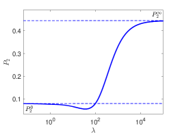
Figure 1: Optimal performance as a function of turnover (log scale). The dashed lines indicate the analytic limits $\lambda\rightarrow 0$ and $\lambda\rightarrow\infty$ computed in Sections VII and VIII.

More specifically, we now consider the following parametric interpolation:

$$s_{1}(y,t)= s_{cc}\cos\left(4\pi^{2}t\right)\cos(2\pi y)+s_{cs}\cos\left(4\pi^{2}t\right)\sin(2\pi y)$$

$$+ s_{sc}\sin\left(4\pi^{2}t\right)\cos(2\pi y)+s_{ss}\sin\left(4\pi^{2}t\right)\sin(2\pi y),$$ (48)

$$u_{1}(y,t)= u_{cc}\cos\left(4\pi^{2}t\right)\cos(2\pi y)+u_{cs}\cos\left(4\pi^{2}t\right)\sin(2\pi y)$$

$$+ u_{sc}\sin\left(4\pi^{2}t\right)\cos(2\pi y)+u_{ss}\sin\left(4\pi^{2}t\right)\sin(2\pi y).$$

The goal now is to find the optimal set of coefficients $s_{i,j}$ and $u_{i,j}$ where the indexes take the values either $c$ or $s$.

We use this ansatz (48) to analytically solve the linear problem (21)-(22) and compute the function $w_{1}(y,t)$. With this information at hand we can directly express the cost (23) and also the performance (24) by explicitly solving the equation (26)-(27). We do not include the corresponding straightforward but cumbersome derivations here. The remaining Karush-Kuhn-Tucker problem of maximizing $P_{2}$ under the constraints $C_{2}=1/2$ (while respecting the inequality constraint (28)) becomes finite dimensional in terms of the height coefficients $s_{i,j}$ and $u_{i,j}$. The structure of the optimal solution can then be studied as a function of the remaining parameter $\lambda$.

In Fig. 1 we show the optimal performance $P_{2}(\lambda)$ computed by numerically solving the optimization problem with an interior-point method for each value of $\lambda$. We observe a gradual transition between the two limiting regimes. Thus, as $\lambda\to 0$ the function $P_{2}(\lambda)$ reaches the value $P_{2}^{0}=1/(4\pi)$ computed analytically in the $\lambda\ll 1$ limit. The corresponding optimal actuation strategy is the purely mechanical driving

$$s_{1}^{0}=-\pi\sqrt{2}\sin(2\pi(2\pi t-y+a))/2$$ (49)

without any chemical driving: $u_{1}^{0}=0$ found in (39). Note that the optimal performance first decays to reach a minimum, but then finally starts to increases reaching eventually the plateau $P_{2}^{\infty}=1/(1/\pi+12\pi-4\sqrt{1+8\pi^{2}})$ computed analytically in the $\lambda\gg 1$ limit. The corresponding optimal actuation agrees with (47), but now, in view of the particular structure of the ansatz, with an explicitly specified time dependent multiplier $\phi(t)=\sqrt{2}\sin\left(4\pi^{2}t+a\right)$. In both limits $a$ is an arbitrary phase.

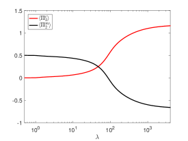
Figure 2: Evolution of the mechanical (black) and chemical (red) costs as a function of the turnover (log scale). The sum of the two costs is maintained at the fixed value $C_{2}=1/2$.

In Fig. 2 we show the contributions of the mechanical $\langle\Pi^{m}_{2}\rangle$ and the chemical $\langle\Pi^{c}_{2}\rangle$ activity to the total energetic cost of self-propulsion $C_{2}=\langle\Pi^{m}_{2}\rangle+\langle\Pi^{c}_{2}\rangle=1/2$. We see that in the regimes with $\lambda\ll 1$ the main energy supply comes from the mechanical source and is represented by the work of the active stresses. Instead, in the regimes with $\lambda\gg 1$ the main energy supply comes from the chemical “pumps” ensuring the appropriate target density of the turnover. Moreover, in those regimes the flux of mechanical energy even changes sign such that mechanical actuators actually work to extract energy from the system (effectively corresponding to a brake on the global motion in the absence of chemical activity). In this way more chemical energy can be injected in. This is a consequence of the constraint fixing the total chemo-mechanical energy input and leaving the system the freedom to self-organize to optimally use this cost.

Another observable feature of the interaction between the mechanical and the chemical actuation is the dip in the performance $P_{2}(\lambda)$ at small to finite values of $\lambda$ with respect to the performance $P_{2}^{0}$ achieved at $\lambda=0$, see Fig. 1. This means that, when first activated, the chemical machinery is detrimental as it interferes with the traveling wave mechanical activation and effectively works as a brake. As the corresponding “chemical engine” gets sufficiently strong, it starts to modify the very regime of actuation from a traveling to a standing wave type, and the performance starts to grow reaching eventually the limit $P_{2}^{\infty}$.

To corroborate this explanation, we show in Fig. 3 the evolution of the optimal performance when we use a restricted actuation ansatz with either $u_{1}=0$ (purely mechanical actuation) or $s_{1}=0$ (purely chemical actuation). As expected, the purely mechanical actuation performance only deteriorates with growing $\lambda$. Indeed, the increase of material turnover still triggers the transition from a traveling to a standing wave for the optimal actuation protocol. But the latter is associated with a decrease of performance in the absence of any active chemical recycling. Instead, the purely chemical optimal actuation, which always takes the form of a standing wave, can take advantage of fast turnover while it is less effective than the purely mechanical actuation for slow turnover. We associate the non-monotony of the optimal performance at small to intermediate values of $\lambda$ to the somewhat arbitrary form of our ansatz (48) in this regime. It is nevertheless interesting that for this specific ansatz, in the limit $\lambda\gg 1$ the purely chemical actuation achieves exactly the same level of performance $P_{2}^{0}$ as the purely mechanical actuation achieves at $\lambda\ll 1$ even if with fundamentally different spatio-temporal pattern: a traveling wave for the mechanical actuation and a standing wave for the chemical actuation.

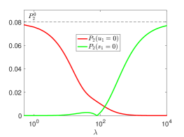
Figure 3: Optimal performances as a function of the turnover with a mechanical driving only (red curve) and with a chemical driving only (green curve). The cost is maintained at the fixed value $C_{2}=1/2$. The dashed line indicates the value of $P_{2}^{0}$.

Another illustration of the progressive transition from a traveling wave type to a standing wave type actuation can be provided if we use (48) to construct an “order parameter” type variable $\theta$, normalized to vanish in the standing wave regime. To this end we first rewrite (48) in the form

$$s_{1}=2s_{0}\cos\left(4\pi^{2}t-\frac{\psi_{-}+\psi_{+}}{2}\right)\cos\left(2\pi y-\frac{\psi_{+}-\psi_{-}}{2}\right)$$

$$+(s_{+}-s_{0})\cos\left(2\pi(2\pi t-y)-\psi_{-}\right)$$

$$+(s_{-}-s_{0})\cos\left(2\pi(2\pi t+y)-\psi_{+}\right),$$

where $s_{0}=\sqrt{s_{cc}^{2}+s_{ss}^{2}+s_{cs}^{2}+s_{sc}^{2}}/2$, $\Delta s=(s_{cc}s_{ss}-s_{cs}s_{sc})/2$, $s_{+}=\sqrt{s_{0}^{2}+\Delta s}$, $s_{-}=\sqrt{s_{0}^{2}-\Delta s}$, $\tan(\psi_{+})=(s_{ss}+s_{cc})/(s_{sc}+s_{cs})$ and $\tan(\psi_{-})=(s_{cc}-s_{ss})/(s_{sc}-s_{cs})$. This representation naturally splits the terms representing a standing wave contribution from the two traveling waves moving, respectively, prograde and retrograde. Note that at $\Delta s=0$, or equivalently $s_{+}=s_{-}=s_{0}$, the traveling wave contribution vanishes. Therefore, the indicator

$$\theta=\frac{(s_{-}-s_{0})^{2}+(s_{+}-s_{0})^{2}}{4s_{0}^{2}}=1-\frac{s_{+}+s_{-}}{2s_{0}}.$$

compares the magnitude of the traveling wave type contributions with the standing wave type contribution while being normalized to vanish in the purely standing wave type regime. The same type of “order parameter” can be constructed using the $u_{1}$ part of the of the ansatz (48) or indeed any linear combination between $u_{1}$ and $s_{1}$.

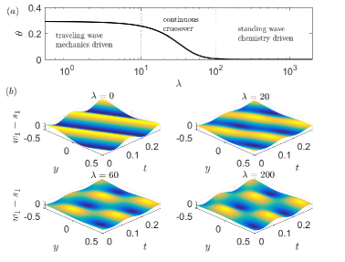
Figure 4: Transition from a traveling wave optimal actuation to a standing wave as $\lambda$ increases. (a) Shows the decay of the order parameter $\theta$ to zero (log scale). (b) displays the spatio-temporal density variations $w_{1}-s_{1}$ in the system at specific values of $\lambda$.

In Fig. 4 we show the behavior of the function $\theta(\lambda)$ in the regimes when both mechanical and chemical actuations are present. In the same figure we illustrate how the spatio-temporal density profile evolves as the parameter $\lambda$ changes from zero to infinity and the traveling wave becomes progressively arrested opening the way to the formation of essentially quiescent nodes separating periodically “breathing” sectors.

As we are dealing only with the simple ansatz (48), the exact evolution of the optimal actuation regime at a finite time scale of the mechanical friction vis a vis the time scale of the chemical relaxation would still have to be obtained for general time periodic controls. For instance, it cannot be excluded that the optimal transition between the two limiting regimes is abrupt rather than continuous, as it is suggested by our finite dimensional approximation. Also, some other spatio-temporal patterns may emerge along the way as one moves from one limiting regimes to another. The rigorous clarification of all these issues which require more intense numerical approaches is left for future studies.

X Conclusions

We have proposed a 1D prototypical model of a chemo-mechanically driven system which can crawl on a solid substrate. While it can be interpreted as a paradigmatic approach to the understanding of how active stress and meshwork remodeling can conspire in living cells, it can also be used as a model of a biomimetic self-propelling soft robot.

The motion is actuated by two time periodic active controls which are fully intrinsic as they exert zero average action on the system. Those two controls are physically fundamentally different, with one being mechanical and the other being chemical. The active mechanical force field is deforming the elastic scaffold while the out of equilibrium mass reservoir actively controls the availability of building blocks of the scaffold.

For our analysis we have chosen a simple close-to-equilibrium framework which enabled us to introduce the turnover kinetic time scale and the characteristic time scale of mechanical relaxation. When the turnover kinetics is slow, the best performance at a fixed energetic cost is achieved by a purely mechanical actuation represented by a traveling wave deformation propagating from the rear to the front of the crawler. Instead, when the turnover kinetics is fast, the best performance is reached when both mechanical and chemical drivings cooperate and form a standing wave.

Our approach also allowed us to study the continuous crossover between the limiting “mechanics dominated” and “chemistry dominated” regimes for a specific actuation ansatz. Here one can expect that in more elaborate models various other intermediate regimes of actuation, characterizing alternative optimal crawling gaits, can become possible with continuous as well as discontinuous transitions between them. The potential complexity of this issue is already suggested by our observation that when the activity of the chemical reservoir is still weak, the associated material turnover represents itself only as a dissipative process which lowers the performance. However, when the chemical activity becomes sufficiently strong, the turnover enhances the performance by offering the possibility to recycle matter without creating a frictional counter-flow. This simple example shows that the optimization of the metabolic actuation may involve a complex interplay between mechanical and chemical active agents and suggests that it is cooperativity of these two mechanisms that ultimately ensures optimality of the self-propulsion machinery.

An important remaining open question is the very possibility to separate the active controls, operating in real living systems, into a purely mechanical actuation and a purely chemical actuation only connected to each other by the constraint that they should operate at a fixed total metabolic cost. In crawling cells both the mechanical activity of molecular motors exerting contractile forces on the polymer network and the chemical activity regulating the turnover of the meshwork through its polymerization and depolymerization are ultimately driven by the same chemical process: the out of equilibrium reaction of ATP hydrolysis. The chemical and mechanical actuations are also tightly dynamically cross-regulated through enzyme coupled receptors [57]. In this way the internal driving mechanisms are also coupled to the dynamics through a system of feedback loops. While all these important processes are left outside the present study, they should become a subject of future work.