Dual-Segment Clustering Strategy for Federated Learning in Heterogeneous Environments

Abstract

Federated learning (FL) is a distributed machine learning paradigm with high efficiency and low communication load, only transmitting parameters or gradients of network. However, the non-independent and identically distributed (Non-IID) data characteristic has a negative impact on this paradigm. Furthermore, the heterogeneity of communication quality will significantly affect the accuracy of parameter transmission, causing a degradation in the performance of the FL system or even preventing its convergence. This letter proposes a dual-segment clustering (DSC) strategy, which first clusters the clients according to the heterogeneous communication conditions and then performs a second clustering by the sample size and label distribution, so as to solve the problem of data and communication heterogeneity. Experimental results show that the DSC strategy proposed in this letter can improve the convergence rate of FL, and has superiority on accuracy in a heterogeneous environment compared with the classical algorithm of cluster.

I Introduction

Traditional distributed machine learning requires clients to share local data, which is not acceptable to everyone[1, 2]. Federated learning (FL) provides a new paradigm that does not require raw data to be shared. Instead, model parameters or gradients are shared, which effectively reduces communication load while preserving data privacy[3]. A commonly used aggregation algorithm for FL is the Federated Averaging (FedAvg) algorithm[4], where a parameter server averages the local parameters or gradients of its clients using the size of the clients’ data as the aggregation weights. In practice, the non-independent and identically distributed (Non-IID) data and the heterogeneity of communication quality can substantially compromise the performance of FL aggregation[5, 6, 7].

Clustering clients before aggregation is an effective way to improve the aggregation efficiency and accuracy of FL. Duan et al.[8] proposed a hierarchical FL framework by setting up a proxy server within a group to aggregate the parameters of the members and then uploading them to the parameter server to update the global parameters. In the hierarchical framework proposed in[9], data quantization and sequence learning were used within groups to improve the aggregation efficiency of FL under Non-IID data setting. Most of the existing grouping methods only alleviate the impact of data heterogeneity on FL aggregation efficiency. The heterogeneity of communication affects the clients’ transmission quality, and hence would also affect the aggregation performance of FL.

Works in [10, 11] designed clustering strategies based on communication cost, but they did not consider the data heterogeneity of each group. The authers of [12, 13, 14] comprehensively captured clients’ communication ability and the heterogeneity of data while clustering. However, they aimed to reduce transmission delay, instead of addressing the impact of communication quality.

Motivated by the above discussion about clustering strategies, this letter proposes a new dual-segment clustering (DSC) strategy to address both the Non-IID characteristics of local data and the heterogeneity of communication quality. First, a signal-to-noise ratio (SNR) matrix is constructed to reflect the communication quality of each client. The initial-clustering is performed according to the similarities among clients. Second, within each primary group, the information quantity matrix of local data distribution is built for secondary-clusters. Finally, for scattered points that remain ungrouped, the principle of Euclidean distance based proximity is adopted to integrate them into their respective nearby groups. By implementing this proposed DSC strategy, the data distribution among the groups exhibits similarity, effectively approximating an IID setting. Additionally, the communication conditions among the clients within the groups remain relatively uniform, significantly enhancing FL aggregation efficiency and accuracy in non-IID scenarios. The DSC algorithm is verified by experiments. To the best of our knowledge, this is the first clustering strategy addressing the heterogeneity of data and the communication quality.

The remainder of this letter is structured in the following manner: Section II illustrates the system modeling, including the group-based FL aggregation and wireless communication. Section III elaborates on the proposed DSC strategy in detail. The simulation results are presented in Section IV. Section V gives the conclusions.

II System Model

Before designing the DSC strategy, the modeling of the system is presented in this section. We consider an FL system consisting of an $N_{a}$-antenna BS (serving as the parameter server) and K single-antenna devices (as clients). The $k$-th device has its own local data set $\mathcal{D}_{k}$. The devices participating in training are indexed by $k=\left\{1,2,\ldots,\ K\right\}$. Consider an FL algorithm with input data vector $\boldsymbol{x}_{ks}\in\mathbb{R}^{d}$ and single output $y_{ks}\in\mathbb{R}$, where $s\in\{1,...,|\mathcal{D}_{k}|\}$. Let $\boldsymbol{w}_{k}$ define the model parameters of the local model trained at the $k$-th device.

II-A Learning Model

For the edge devices, the goal of local training is to find the optimal learning model $\boldsymbol{w}^{\ast}$ that minimizes its training loss. Without loss of generality, the local gradient of the model parameter $\boldsymbol{w}\in\mathbb{R}^{q}$ (where $q$ denotes the model size) on $\mathcal{D}_{k}$ in the $t$-th communication round is defined as

$$\nabla F_{k}\left(\boldsymbol{w}^{[t]}\right)=\frac{1}{|\mathcal{D}_{k}|}\sum_{\left(\boldsymbol{x}_{ks},y_{ks}\right)\in\mathcal{D}_{k}}\nabla f_{k}\left(\boldsymbol{x}_{ks},y_{ks};\boldsymbol{w}^{[t]}\right),$$ (1)

where $f_{k}\left(\boldsymbol{x}_{ks},y_{ks};\boldsymbol{w}\right)$ denotes the sample loss. For brevity, we rewrite $f_{k}\left(\boldsymbol{x}_{ks},y_{ks};\boldsymbol{w}\right)$ as $f_{k}\left(\boldsymbol{w}\right)$.

To achieve the minimum global loss function, FL conducts multiple rounds of gradient transmission until convergence. In this letter, clustering is performed among the clients before updating. Thus, at each communication round, the gradients from clients within each groups are first synchronously aggregated by the group leaders $l=\{1,2,\dots,L\}$ as

$$\nabla F_{l}\left(\boldsymbol{w}^{[t]}\right)=\sum_{k=1}^{K_{l}}G_{k}\cdot\nabla F_{k}\left(\boldsymbol{w}^{[t]}\right),$$ (2)

where $l$ is the index of a group leader, $G_{k}$ is the intra-group aggregation weight of client $k$, and $K_{l}$ represents the number of clients within the $l$-th group satisfying $K=\sum_{l=1}^{L}{K_{l}}$. Then, the BS aggregates the gradients from each group leader, as given by

$$\nabla F\left(\boldsymbol{w}^{[t]}\right)=\sum_{l=1}^{L}G_{l}\cdot\nabla F_{l}\left(\boldsymbol{w}^{[t]}\right).$$ (3)

where $G_{l}$ is the inter-group aggregation weight of group leader $l$.

Each group include as many sample labels as possible, so an aggregation weight dedicated to the Non-IID case[15] is used within the group due to the large difference in the data distribution, as given by

$$G_{k}=\frac{|\mathcal{D}_{k}|e^{f(\theta_{k}^{[t]})}}{\sum_{i=1}^{K_{l}}{|\mathcal{D}_{i}|e^{f(\theta_{i}^{[t]})}}},$$ (4)

where $f(\theta_{i}^{[t]})=1-e^{-e^{-(\theta_{i}^{[t]}-1)}}$, and $\theta_{i}^{[t]}=arccos\frac{\langle\nabla F_{l}\left(\boldsymbol{w}^{[t]}\right),\nabla F_{k}\left(\boldsymbol{w}^{[t]}\right)\rangle}{\|\nabla F_{l}\left(\boldsymbol{w}^{[t]}\right)\|\cdot\|\nabla F_{k}\left(\boldsymbol{w}^{[t]}\right)\|}$. $G_{l}=|\mathcal{D}_{l}|/\sum_{l=1}^{L}{|\mathcal{D}_{l}|}$ is used for the small difference among the groups.

Finally, the update of the global model implemented at the BS is given by

$$\boldsymbol{w}^{[t+1]}=\boldsymbol{w}^{[t]}-\lambda\cdot\nabla F\left(\boldsymbol{w}^{[t]}\right),$$ (5)

where $\lambda$ is the learning rate.

II-B Communication Model

Non-Orthogonal Multiple Access (NOMA) [16] is considered in this letter to support multiple users and the BS to transmit data simultaneously through superimposed wireless channels, effectively alleviating the communication network congestion caused by multiple users in FL [17]. No inter-client interference is considered in this letter.

Consider a block fading channel, where the channel coefficients remain invariant during the whole FL training process. Let $\boldsymbol{h}_{k}\in\mathbb{C}^{N}$ denote the channel coefficient vector of the direct channel from the $k$-th-device to the BS, and the amplitudes are the independent Rician random variables. Assume perfect channel state information (CSI) at the BS and devices. Thus, in the model aggregation of the $t$-th communication round, the received signal is denoted by

$$\boldsymbol{y}^{\left[t\right]}=\sum_{l=1}^{K}{\boldsymbol{h}_{l}p_{l}\boldsymbol{s}_{l}^{\left[t\right]}}+\boldsymbol{n}_{0},$$ (6)

where $p_{l}\in\mathbb{C}$ is the transmitter scalar of the $l$-th group leader, $\boldsymbol{s}_{l}$ is the gradient at the $l$-th group leader aggregated from the group members, and $\boldsymbol{n}_{0}\in\mathbb{C}^{N\times 1}$ is the additive white Gaussian noise (AWGN) vector with the entries following $\mathcal{CN}\left(0,\sigma_{n_{0}}^{2}\right)$. In fact, the transmit power of each client is set to be the same in this letter.

The SNR is used to measure the communication quality, which is heterogeneous due to the geograpgic distribution of the clients. Let $\gamma_{k}=p_{k}|\boldsymbol{h}_{k}|^{2}/\sigma_{n_{0}}^{2}$ represent the received SNR from the $k$-th client to the BS. Meanwhile, if the gradient transmission among the clients is completed according to the above communication mode, then $\gamma_{jk}=p_{k}|h_{jk}|^{2}/\sigma_{n_{0}}^{2}$ represents the received SNR when the $k$-th client transmits the gradients to the $i$-th client, where $h_{jk}$ is the channel coefficient between the $k$-th and $j$-th client.

III Proposed Dual-Segment Clustering Strategy

In this section, we elaborate on the new DSC strategy, which is divided into two parts: 1) The primary groups are obtained by clustering based on the heterogeneity of communication quality. 2) The secondary groups are established within each primary group through the proposed information matrix of data distribution so that each secondary group contains as many sample labels as possible. The group members transmit the gradients to the group leaders, see (2), and the group leaders upload the aggregated gradients in the groups to the BS, see (3). The framework is showed in Fig. 1.

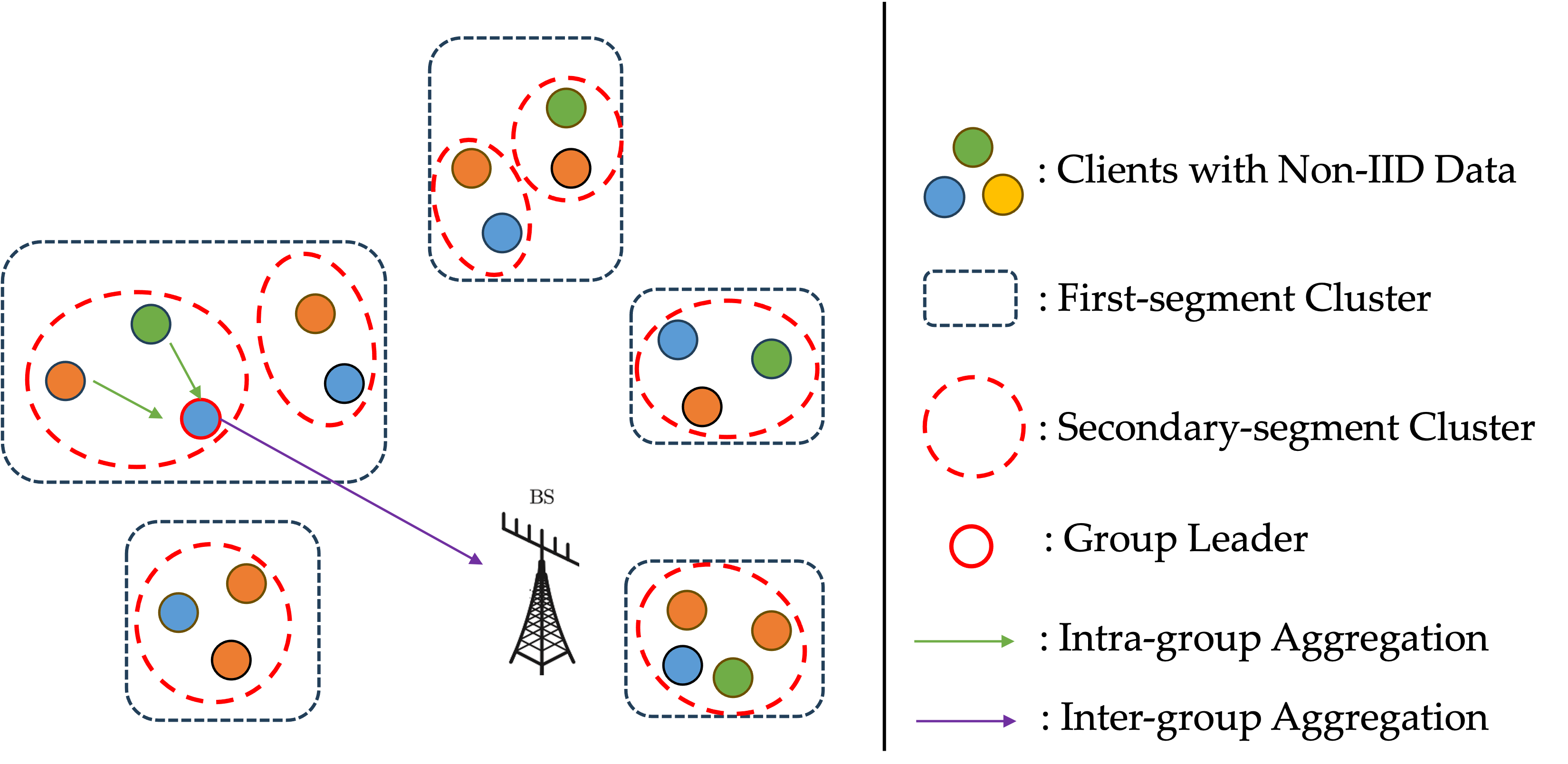
Figure 1: The workflow of proposed DSC-FL.

III-A Cluster based on Communication quality

The FL system in this letter adopts a synchronous upload mechanism, where the BS reserves a fixed window period for each client to upload its local model in each communication round. Assume that the geographical location and transmission power of all clients are fixed, that is, their communication quality does not change over iterations. As mentioned in Section II-B, the SNR of each client can directly reflect the communication quality and their heterogeneity. Therefore, we first construct the SNR matrix, as given by

$$\Gamma=\begin{bmatrix}\gamma_{1}&\gamma_{12}&\cdots&\gamma_{1K}\\ \gamma_{21}&\gamma_{2}&\cdots&\gamma_{2K}\\ \vdots&\vdots&\ddots&\vdots\\ \gamma_{K1}&\gamma_{K2}&\cdots&\gamma_{K}\end{bmatrix},$$ (7)

where the diagonal elements represent the SNR between the clients and the BS, while the element in the $i$-th row and the $j$-th column represent the SNR between the $i$-th and $j$-th clients. $\Gamma$ is a symmetric matrix where the SNRs are measured by transmitting gradients among the clients and from the client to the BS in the first communication round.

It is worth noting that FL generally is suitable for different training tasks and adapt to different wireless communication environments. The data and communication conditions of the clients are unpredictable, so the clustering algorithm should not have a priori knowledge of the number of classes, which is different from most existing FL clustering methods.

A similarity matrix $S_{c}$ is constructed based on the SNR to describe the similarity between the clients in terms of their communication quality, i.e.,

$$S_{c}=\begin{bmatrix}P_{1}&-\gamma^{2}_{12}&\cdots&-\gamma^{2}_{1K}\\ -\gamma^{2}_{21}&P_{2}&\cdots&-\gamma^{2}_{2K}\\ \vdots&\vdots&\ddots&\vdots\\ -\gamma^{2}_{K1}&-\gamma^{2}_{K2}&\cdots&P_{K}\end{bmatrix},$$ (8)

where $\{P_{1},P_{2},\cdots,P_{K}\}$ is the preference value for communication quality, implying the likelihood of that client $k=\left\{1,2,\ldots,\ K\right\}$ being the center of the group, affecting the number of groups. Let the responsibility matrix $R_{c}(i,k)$ represent the likelihood of client $k$ being the group leader of client $i$ relative to other data clients. Let the attribution matrix $A_{c}(i,k)$ represent the appropriateness of client $i$ choosing client $k$ as the group leader considering the preference of other clients choosing client $k$ as the group leader. They are both initialized as 0 matrices.

Algorithm 1 The Proposed Dual-Segment Clustering Strategy.

1:  Parameter: The number of samples $|\mathcal{D}_{k}|$ and labels $\mathcal{C}_{k}^{\iota}$ of each client, the responsibility matrix $R_{c_{0}}$ and $R_{d_{0}}$, the attribution matrix $A_{c_{0}}$ and $A_{d_{0}}$, and the learning rate $\lambda$.

2:  

3:  Cluster based on the communication quality:

4:   Calculate $\Gamma$ by (7) and $S_{c}$ by (8):

5:   for $t_{cl}$ in $T_{cl}$ do

6:    Calculate $R_{c}$ by (9).

7:    Calculate $A_{c}$ by (10) and (11).

8:   end for

9:   Return $l_{com}$ primary groups.

10:   Data-based Cluster within $l_{com}$ primary groups:

11:    Calculate $\Xi$ by (12) and $S_{d}$ by (13):

12:    for $t_{cl}$ in $T_{cl}$ do

13:     Calculate $R_{d}$ by the same way as (9).

14:     Calculate $A_{d}$ by the same way as (10) and (11).

15:    end for

16:  

17:  for $t\leftarrow\{0,1,2,\dots,T\}$ do

18:     Intra-group aggregation by (2).

19:     Inter-group aggregation by (3).

20:     Update the global model by (5) and broadcast to each client.

21:  end for

22:  Return $\boldsymbol{w}$.

The clustering algorithm iterates over $R_{c}(i,k)$ and $A_{c}(i,k)$ until the group boundaries remain unchanged after $T_{cl}$ iterations (e.g., we set $T_{cl}=15$ in this letter). The responsibility information is updated according to

$$R_{c}(i,k)=S_{c}(i,k)-\max_{k\neq k^{\prime}}{[S_{c}(i,k^{\prime})+A_{c}(i,k^{\prime})]},$$ (9)

and the attribution information according to

$$A_{c}(i,k)=\min[0,R_{c}(k,k)+\sum_{i^{\prime}\notin(i,k)}{\max(0,R_{c}(i^{\prime},k))}],i\neq k$$ (10)

and

$$A_{c}(i,i)=\max_{i^{\prime}\neq k}{[0,R_{c}(i^{\prime},k)]},i=k.$$ (11)

The responsibility information and attribution information can be combined to determine how suitable the client $i$ is as a cluster center or group member. The clients whose indices correspond to the elements on the diagonal of $C_{c}=R_{c}(i,k)+A_{c}(i,k)$ are suitable as cluster centers. Specifically, if the maximum element of the $i$-th row in $C_{c}$ is in the diagonal position, the $i$-th client is the cluster center (i.e., the group leader) corresponding to the column index. Otherwise, the $i$-th client is classified as a member of the group indexed by the column corresponding to the maximum element.

III-B Secondary Cluster based on Non-IID Data

After clustering based on the heterogeneity of communication quality in Section III-A, the accuracy of gradient transmission within each primary group is guaranteed when intra-group aggregation. Next, we continue to cluster clients according to data heterogeneity within each primary group, to make the clients contain as many class of sample label as possible in each secondary cluster.

Consider $K$ clients in the FL system contain a total of $\mathcal{D}$ data samples and $\mathcal{L}$ labels. The number of the $\iota$-th label of the $k$-th client is $\mathcal{C}_{k}^{\iota}$. The total number of label is $\mathcal{C}^{\iota}$. For any sample, the probability that the sample belongs to the $\iota$-th class label in the data of the $k$-th client is $P_{1}=\mathcal{C}_{k}^{\iota}/\mathcal{D}$, the probability of it belonging to the $k$-th client is $P_{2}=\mathcal{D}_{k}/\mathcal{D}$, and the probability of it belonging to the $\iota$-th class label is $P3=\mathcal{C}^{\iota}/\mathcal{D}$. Based on these settings, a matrix measuring the distribution of dataset can be written as

$$\Xi=-\begin{bmatrix}\frac{\mathcal{C}_{1}^{1}}{\mathcal{D}}\log{\frac{\mathcal{D}\mathcal{C}_{1}^{1}}{\mathcal{D}_{1}\mathcal{C}^{1}}}&\frac{\mathcal{C}_{1}^{2}}{\mathcal{D}}\log{\frac{\mathcal{D}\mathcal{C}_{1}^{2}}{\mathcal{D}_{1}\mathcal{C}^{2}}}&\cdots&\frac{\mathcal{C}_{1}^{\mathcal{L}}}{\mathcal{D}}\log{\frac{\mathcal{D}\mathcal{C}_{1}^{\mathcal{L}}}{\mathcal{D}_{1}\mathcal{C}^{\mathcal{L}}}}\\ \frac{\mathcal{C}_{2}^{1}}{\mathcal{D}}\log{\frac{\mathcal{D}\mathcal{C}_{2}^{1}}{\mathcal{D}_{2}\mathcal{C}^{1}}}&\frac{\mathcal{C}_{2}^{2}}{\mathcal{D}}\log{\frac{\mathcal{D}\mathcal{C}_{2}^{2}}{\mathcal{D}_{2}\mathcal{C}^{2}}}&\cdots&\frac{\mathcal{C}_{2}^{\mathcal{L}}}{\mathcal{D}}\log{\frac{\mathcal{D}\mathcal{C}_{2}^{\mathcal{L}}}{\mathcal{D}_{2}\mathcal{C}^{\mathcal{L}}}}\\ \vdots&\vdots&\ddots&\vdots\\ \frac{\mathcal{C}_{K}^{1}}{\mathcal{D}}\log{\frac{\mathcal{D}\mathcal{C}_{K}^{1}}{\mathcal{D}_{K}\mathcal{C}^{1}}}&\frac{\mathcal{C}_{K}^{2}}{\mathcal{D}}\log{\frac{\mathcal{D}\mathcal{C}_{K}^{2}}{\mathcal{D}_{K}\mathcal{C}^{2}}}&\cdots&\frac{\mathcal{C}_{K}^{\mathcal{L}}}{\mathcal{D}}\log{\frac{\mathcal{D}\mathcal{C}_{K}^{\mathcal{L}}}{\mathcal{D}_{K}\mathcal{C}^{\mathcal{L}}}}\end{bmatrix},$$ (12)

where $\frac{\mathcal{C}_{k}^{\iota}}{\mathcal{D}}\log{\frac{\mathcal{D}\mathcal{C}_{k}^{\iota}}{\mathcal{D}_{k}\mathcal{C}^{\iota}}}$ represents the information amount of the event that a sample belongs to the $\iota$-th label of the $k$-th client. Based on $\Xi$, we construct a similarity matrix that describes the distribution of the dataset,i.e.,

$$S_{d}=\begin{bmatrix}P_{d}&s_{1,2}&\cdots&s_{1,K_{l_{com}}}\\ s_{2,1}&P_{d}&\cdots&s_{2,K_{l_{com}}}\\ \vdots&\vdots&\ddots&\vdots\\ s_{K_{l_{com}},1}&s_{K_{l_{com}},2}&\cdots&P_{d}\end{bmatrix},$$ (13)

where $s_{i,k}=\{\sum_{\iota=1}^{\mathcal{L}}{[\Xi(i,\iota)-\Xi(k,\iota)]^{2}}\}^{2}$ with $i\neq k$, ${P}_{d}$ is the preference value for data distribution, and $K_{l_{com}}$ denotes the number of clients in the $l_{com}$-th primary group.

Similarly, we also define the responsibility matrix $R_{d}(i,k)$and the attribution matrix $A_{d}(i,k)$ for $S_{d}$ to iteratively update the secondary-segment group based on data heterogeneity, as the final cluster of the FL system in this letter. For clients that are not grouped, we assign them to the nearest group according to the nearest principle.

The proposed DSC strategy is summarized in Algorithm 1.

IV Simulation Results

IV-A Simulation Setup and Baselines

Consider a rectangular area with a length of 100 meters. 50 clients and a BS as the parameter server are randomly distributed in the area. The path loss model is $PL_{DB}=G_{BS}G_{D}{(\frac{c}{4\pi f_{c}d_{DB}})}^{P}$, where $G_{BS}=5$ dBi for the BS and $G_{D}=0$ dBi for clients represent antenna gain, $f_{c}=915$ MHz represents the carrier frequency, $P=3.76$ is path loss coefficient, $d$ is the distance, and $c$ is the speed of light. The transmit power of the client is $10^{-4}$ W and the noise power is $10^{-6}$ W. We use a CNN network with two $5\times 5$ convolution layers (each with $2\times 2$ max pooling) followed by a batch normalization layer, a fully connected layer with 50 units, a ReLu activation layer, and a softmax output layer, for training and testing on MNIST dataset and Fashion-MNIST dataset, respectively. The data is randomly distributed to the clients with each client assigned 400-800 samples of two random labels. The SGD algorithm with $batchsize=0.1$ is used to train the local model. The learning rate is $\lambda=0.06$ for the MNIST dataset and 0.05 for the Fashion-MNIST dataset.

We test the performance of the DSC algorithm proposed in this letter (Setting 1) and the data-based clustering part of the proposed DSC algorithm (Setting 2), in FL. For comparison, we set two baselines: 1) The state-of-the-art typical clustering algorithm (Benchmark 1) [18], and 2) The most widely used FedAvg algorithm (Benchmark 2)[4].

IV-B The Effectiveness and Superiority of DSC-FL

The four baselines are tested in an ideal communication environment (without noise) and an actual communication environment (with noise). It is worth mentioned that Setting 1 is not required for the ideal communication environment due to the fact that there is no need for clustering based on communication quality.

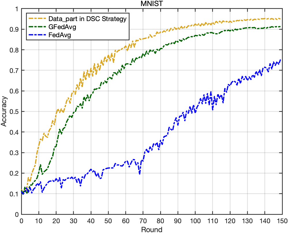
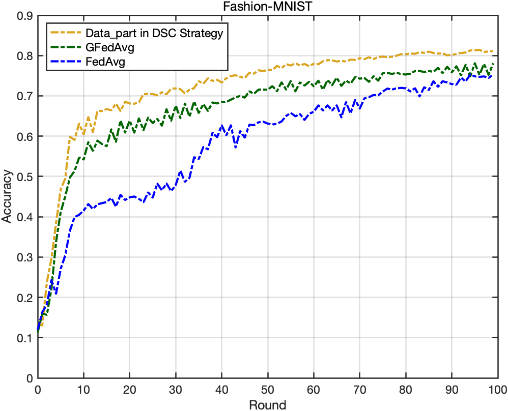
Figure 2: The performance of FL after clustering in an ideal communication environment.

Fig. 2 shows the performance of Setting 2 and Benchmarks 1, 2 in the ideal communication environment. First, the algorithm of Setting 2 outperforms FedAvg algorithm (Benchmark 2) on both two datasets by 19.74% (MNIST) and 5.91% (Fashion-MNIST), respectively, which proves the effectiveness of the data-based clustering part of the proposed DSC algorithm. Second, compared with the performance of the existing algorithm (Benchmark 1), it can be seen that the performance of proposed algorithm is significantly higher than that of the existing algorithm by 3.71% (MNIST) and 3.03% (Fashion-MNIST), respectively, in the ideal communication environment, which proves the superiority of the data-based clustering part of the proposed DSC algorithm.

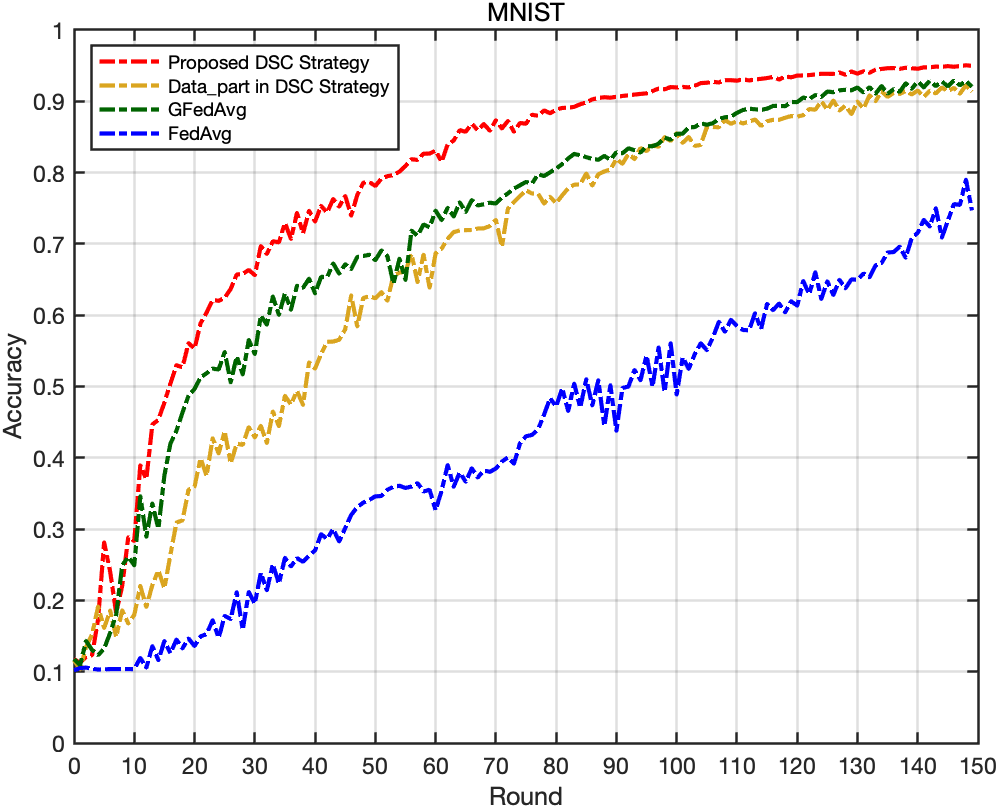
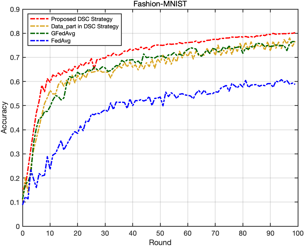
Figure 3: The performance of FL after clustering in an actual communication environment.

Fig. 3 illustrates the FL performance using 4 algorithms in the real communication environment. First, compared with FedAvg algorithm (Benchmark 2), the performance of DSC algorithm (Setting 1) and its data part (Setting 2) are improved by 20.28% (MNIST), 21.42% (Fashion-MNIST) and 16.66% (MNIST), 17.89% (Fashion-MNIST), respectively. The effectiveness of the proposed DSC algorithm in the actual communication environment is proved. Second, the complete DSC algorithm (Setting 1) improves the performance by 2.92% on MNIST and 3.68% on Fashion-MNIST compared with the GFedAvg algorithm (Benchmark 1), although the performance of its data part (Setting 2) is not greatly higher than that of the GFedAvg algorithm in noisy environments. The importance and superiority of the DSC strategy proposed in this letter are demonstrated.

V Conclusion

In this letter, a DSC strategy is proposed considering the heterogeneity of both data and communication quality, which comprehensively improves the convergence rate and accuracy of FL in an actual heterogeneous environment. The optimal configuration of communication and computing resources is not involved in the proposed system, which will be taken as the next work to further improve the availability of FL in practical environments on the basis of efficient aggregation.

References

- [1] J. Dean, G. Corrado, R. Monga, K. Chen, M. Devin, M. Mao, M. Ranzato, A. Senior, P. Tucker, K. Yang et al., “Large scale distributed deep networks,” Advances in neural information processing systems, vol. 25, 2012.
- [2] M. Li, D. G. Andersen, J. W. Park, A. J. Smola, A. Ahmed, V. Josifovski, J. Long, E. J. Shekita, and B.-Y. Su, “Scaling distributed machine learning with the parameter server,” in 11th USENIX Symposium on operating systems design and implementation (OSDI 14), pp. 583–598, 2014.
- [3] J. Konečnỳ, B. McMahan, and D. Ramage, “Federated optimization: Distributed optimization beyond the datacenter,” arXiv preprint arXiv:1511.03575, 2015.
- [4] B. McMahan, E. Moore, D. Ramage, S. Hampson, and B. A. y Arcas, “Communication-efficient learning of deep networks from decentralized data,” in Artificial intelligence and statistics, pp. 1273–1282. PMLR, 2017.
- [5] T.-M. H. Hsu, H. Qi, and M. Brown, “Measuring the effects of non-identical data distribution for federated visual classification,” arXiv preprint arXiv:1909.06335, 2019.
- [6] K. Hsieh, A. Phanishayee, O. Mutlu, and P. Gibbons, “The non-iid data quagmire of decentralized machine learning,” in International Conference on Machine Learning, pp. 4387–4398. PMLR, 2020.
- [7] Y. Zhao, M. Li, L. Lai, N. Suda, D. Civin, and V. Chandra, “Federated learning with non-iid data,” arXiv preprint arXiv:1806.00582, 2018.
- [8] M. Duan, D. Liu, X. Chen, R. Liu, Y. Tan, and L. Liang, “Self-balancing federated learning with global imbalanced data in mobile systems,” IEEE Transactions on Parallel and Distributed Systems, vol. 32, no. 1, pp. 59–71, 2020.
- [9] S. Seo, J. Lee, H. Ko, and S. Pack, “Performance-aware client and quantization level selection algorithm for fast federated learning,” in 2022 IEEE Wireless Communications and Networking Conference (WCNC), pp. 1892–1897. IEEE, 2022.
- [10] L. Liu, J. Zhang, S. Song, and K. B. Letaief, “Client-edge-cloud hierarchical federated learning,” in ICC 2020-2020 IEEE international conference on communications (ICC), pp. 1–6. IEEE, 2020.
- [11] C. Wang, Y. Yang, and P. Zhou, “Towards efficient scheduling of federated mobile devices under computational and statistical heterogeneity,” IEEE Transactions on Parallel and Distributed Systems, vol. 32, no. 2, pp. 394–410, 2020.
- [12] J.-w. Lee, J. Oh, Y. Shin, J.-G. Lee, and S.-Y. Yoon, “Accurate and fast federated learning via iid and communication-aware grouping,” arXiv preprint arXiv:2012.04857, 2020.
- [13] Y. Lei, L. Yanyan, C. Jiannong, H. Jiaming, and Z. Mingjin, “E-tree learning: A novel decentralized model learning framework for edge ai,” IEEE Internet of Things Journal, vol. 8, no. 14, pp. 11 290–11 304, 2021.
- [14] Z. He, L. Yang, W. Lin, and W. Wu, “Improving accuracy and convergence in group-based federated learning on non-iid data,” IEEE Transactions on Network Science and Engineering, vol. 10, no. 3, pp. 1389–1404, 2022.
- [15] H. Wu and P. Wang, “Fast-convergent federated learning with adaptive weighting,” IEEE Transactions on Cognitive Communications and Networking, vol. 7, \hrefhttp://dx.doi.org/10.1109/TCCN.2021.3084406DOI 10.1109/TCCN.2021.3084406, no. 4, pp. 1078–1088, 2021.
- [16] G. Zhu and K. Huang, “Mimo over-the-air computation for high-mobility multimodal sensing,” IEEE Internet of Things journal, vol. 6, no. 4, pp. 6089–6103, 2018.
- [17] W. Ni, Y. Liu, Z. Yang, H. Tian, and X. Shen, “Integrating over-the-air federated learning and non-orthogonal multiple access: What role can ris play?” IEEE Transactions on Wireless Communications, vol. 21, no. 12, pp. 10 083–10 099, 2022.
- [18] W. Nie, L. Yu, and Z. Jia, “Research on aggregation strategy of federated learning parameters under non-independent and identically distributed conditions,” in 2022 4th International Conference on Applied Machine Learning (ICAML), pp. 41–48. IEEE, 2022.