Fair Generalized Linear Mixed Models

Abstract.

When using machine learning for automated prediction, it is important to account for fairness in the prediction. Fairness in machine learning aims to ensure that biases in the data and model inaccuracies do not lead to discriminatory decisions. E.g., predictions from fair machine learning models should not discriminate against sensitive variables such as sexual orientation and ethnicity. The training data often in obtained from social surveys. In social surveys, oftentimes the data collection process is a strata sampling, e.g. due to cost restrictions. In strata samples, the assumption of independence between the observation is not fulfilled. Hence, if the machine learning models do not account for the strata correlations, the results may be biased. Especially high is the bias in cases where the strata assignment is correlated to the variable of interest. We present in this paper an algorithm that can handle both problems simultaneously, and we demonstrate the impact of stratified sampling on the quality of fair machine learning predictions in a reproducible simulation study.

1. Introduction

With the advent of automatic decision-making, the need for fair decision-making algorithms is steadily rising. The automatic decision should comply to restriction based on societal values, such as non-discrimination of parts of the population. Machine learning algorithms, while offering efficiency, can inadvertently perpetuate bias in critical areas like loan approvals ([21]) and criminal justice ([23]). In loan applications, factors like marital status can lead to unfair disadvantages for single individuals, while in criminal justice, algorithms might associate race with recidivism risk, leading to discriminatory sentencing despite individual circumstances. This highlights the need for fair and unbiased AI frameworks to ensure equal opportunities and outcomes for all.

The training data, used to learn the machines for the automatic decision-making, oftentimes comes from surveys. These surveys typically are drawn according to a sampling plan, and hence do not comply with the general assumption in machine learning, that each unit is sampled independently and with the same probability of inclusion. For a detailed discussion on survey methods including sampling strategies, see [31].

The field of fair machine learning has thrived, with numerous research articles exploring approaches to mitigate bias in various algorithms. Notable examples include fair versions of Logistic and Linear Regression ([5]), Support Vector Machines ([35]), Random Forests ([43]), Decision Trees ([1]), and Generalized Linear Models (GLMs) ([22]). These methods aim to address potential discrimination arising from historical data or algorithmic design, ensuring fairer outcomes for all individuals.

In this paper we propose a Generalized Mixed Model for fair predictions. We show how to estimate the model and evaluate its performance against the current model that does not take the possible clustering of the data into account. As far as we know, this has not been proposed before.

The paper is organized as follows: In Section 2 we establish the theoretical underpinnings of fair generalized linear mixed models and propose a strategy for solving them. In Section 3, we conduct a comprehensive evaluation of our proposed method’s effectiveness through various tests. Finally, in Section 4, we demonstrate the practical applicability of our algorithm by solving a real-world problem using the Bank marketing dataset ([32]). Our key findings and potential future directions are presented in Section 5.

2. Fair Generalized Linear Mixed Models

In recent years, there has been a growing interest in developing fair machine learning algorithms. Fairness is a complex concept, but it generally refers to the idea that algorithms should not discriminate against certain groups of people ([17]). This is important because algorithms are increasingly being used to make decisions about people’s lives, such as whether to grant them a loan or admit them to college.

Fair Generalized Linear Mixed Models (GLMMs) are a type of GLMM that has been designed to be fair. They do this by incorporating constraints that ensure that the model’s predictions are not biased against any particular group of people.

2.1. Fair Predictions

In classification algorithms, we need to find a function that predicts the label $y$ given a feature vector $x\in\mathbb{R}^{p}$. This function is learned on a training set $D={(x^{\ell},y_{\ell})}^{N}_{\ell=1}$. One typically way to do that is minimizing a loss function $L(\beta)$ over a training set that minimize the classification error in this set.

In the context of fairness in binary classification, each observation $\ell$ has an associated sensitive feature $s_{\ell}\in\{0,1\}$, and the objective then becomes finding a solution with good accuracy (AC) while it is also fair. The concept of fairness in machine learning can be seen from different metrics, here, we will study the concept of disparate impact (DI) ([2]). Other unfairness metrics for binary classifiers can be found in [42].

A classifier does not suffer from disparate impact if the probability of his prediction is the same for both values of the sensitive feature $s$, that is,

$$\mathbb{E}(y_{\ell}|s_{\ell}=0)=\mathbb{E}(y_{\ell}|s_{\ell}=1).$$

We can also say that an algorithm suffers from disparate impact if the decision-making process grants a disproportionately large fraction of beneficial outcomes to certain sensitive feature groups.

In this context, we have Generalized Linear Models (GLMs) that are a class of models that can be used to model a variety of response variables, including count, continuous and binary data that will be the focus of this work. Following the same idea, but with some changes, we have the Generalized Linear Mixed Models that allow for the inclusion of random effects, which are random variables that capture the variability in the response variable due to the hierarchical data structure. GLMMs are a powerful tool for analyzing data that are non-normal and hierarchical. They are used in a wide variety of fields, including medicine, psychology ([10, 16]) for example. However, GLMMs, like many other statistical models, can lead to unfair outcomes.

2.2. Generalized linear mixed model

Generalized linear mixed models are regarded as an extension of generalized linear models that effectively incorporate random effects. These random effects can come from a survey that has strata bias, for example. This section provides a brief explanation of how we can model the GLMMs as can be seen in [38].

Let $y_{i_{j}}$ denote the label in the observation $j$ in strata $i$, where $i\leavevmode\nobreak\ \in\leavevmode\nobreak\ [1,n]\leavevmode\nobreak\ :=\leavevmode\nobreak\ \{1,\dots,n\}$ and $j\leavevmode\nobreak\ \in\leavevmode\nobreak\ [1,T_{i}]$, with $T_{i}$ being the size of the strata $i$. These observations are collected in the vector $y^{\top}_{i}\leavevmode\nobreak\ =\leavevmode\nobreak\ (y_{i_{1}},\dots,y_{i_{T_{i}}})$. Let $(x^{i_{j}})^{\top}\leavevmode\nobreak\ =\leavevmode\nobreak\ (x^{i_{j}}_{1},\dots,x^{i_{j}}_{p})$ represent the covariate vector associated with fixed effects, and $(z^{i_{j}})^{\top}=(z^{i_{j}}_{1},\dots,z^{i_{j}}_{n})\in\mathbb{R}^{n}$ denote the covariate vector associated with the random effects $b_{i}\leavevmode\nobreak\ \in\leavevmode\nobreak\ [1,n]$ that follow a normal distribution with a covariance matrix $Q_{b}=Blockdiag(Q,\dots,Q)\in\mathbb{R}^{n\times n}$.

The generalized linear mixed model can be expressed as follows:

$$g(\mu_{i_{j}})=\beta_{0}+\beta^{\top}x^{i_{j}}+(z^{i_{j}})^{\top}b_{i}.$$ (1)

Here, $g$ represents a monotonic and continuously differentiable link function, $\mu_{i_{j}}=E(y_{i_{j}}|b_{i},x^{i^{j}},z^{i^{j}})$, $\beta_{0}$ is the intercept, $\beta$ the fixed effects and $b_{i}$ represents the strata-specific random effects.

We can represent Model (1) using matrix notation. Let $(X^{i})^{\top}\leavevmode\nobreak\ =\leavevmode\nobreak\ [x^{i_{1}},\dots,x^{i_{T_{i}}}]\leavevmode\nobreak\ \in\leavevmode\nobreak\ \mathbb{R}^{p\times T_{i}}$ denote the design matrix for the $i$-th strata, and $\tilde{\beta}^{\top}=(\beta_{0},\beta^{\top})$ represent the linear parameter vector, including the intercept. Let $\tilde{X}^{i}=[\mathds{1},X^{i}]\in\mathbb{R}^{(p+1)}$ be the corresponding matrix, where $\mathds{1}^{\top}=(1,\dots,1)\in\mathbb{R}^{T_{i}}$. By grouping the observations within each strata, the model can be represented as:

$$g(\mu_{i})=\tilde{X}^{i}\tilde{\beta}+Z^{i}b_{i},$$

where $(Z^{i})^{\top}=[z^{i_{1}},\dots,z^{i_{T_{i}}}]\in\mathbb{R}^{n\times T_{i}}$. For all observations one obtains

$$g(\mu)=\tilde{X}\tilde{\beta}+Zb,$$

with $\tilde{X}=[\tilde{X}^{1},\dots,\tilde{X}^{n}]\in\mathbb{R}^{N\times(p+1)}$ and a block-diagonal matrix $Z\leavevmode\nobreak\ =\leavevmode\nobreak\ [Z^{1},\dots,Z^{n}]\in\mathbb{R}^{N\times n}$, considering, w.l.o.g., that the first $T_{1}$ points, of $\tilde{X}$ belong to strata $1$, the next $T_{2}$ points belong to strata $2$, and so on, that is, there is an ordering, by strata, in the data.

For $r\in[1,p]$ and $i\in[1,n]$, let us introduce the notation $(x^{i})^{\top}_{r}\leavevmode\nobreak\ =\leavevmode\nobreak\ (x^{i_{1}}_{r},\dots,x^{i_{T_{i}}}_{r})\in\mathbb{R}^{T_{i}}$ to represent the covariate vector of the $r$-th fixed effect in strata $i$. Furthermore, we define $x^{\top}_{r}=((x^{1})^{\top}_{r},\dots,(x^{n})^{\top}_{r})\in\mathbb{R}^{N}$. Consequently, the $r$-th design matrix, which includes the intercept and solely the $r$-th covariate vector, can be expressed as:

$$X^{i}_{r}=[\mathds{1},x^{i}_{r}]\in\mathbb{R}^{T_{i}\times 2}$$

and

$$X_{r}=[\tilde{\mathds{1}},x_{r}]\in\mathbb{R}^{N\times 2},$$

with

$$\tilde{\mathds{1}}=(1,\dots,1)\in\mathbb{R}^{N}$$

representing the design matrices for stratas $i$ and the entire sample, respectively. Within strata $i$, the predictor that exclusively contains the $r$-th covariate takes the form of $\eta^{i}_{r}=X^{i}_{r}\tilde{\beta}_{r}+Z^{i}b_{i}$, where $\tilde{\beta}^{\top}_{r}=(\beta_{0},\beta_{r})\in\mathbb{R}^{2}$. For the entire sample, we obtain:

$$\eta_{r}=X_{r}\tilde{\beta}_{r}+Zb$$

and

$$\eta^{i}=X^{i}\beta+Z^{i}b_{i}.$$

Ignoring the mixed effects we can state that the logistics regression is a special case of GLMs. In the next chapters, we will see this case and some of its particularities for the case in which we have unfair datasets.

2.3. Fair Logistic Regression

In classification algorithms that employ logistic regression that can be seen in [33], a probabilistic model is used to link a feature vector $x$ to the class labels $y\in\{0,1\}$. The link function is:

$$p(\hat{y}=1|x,\beta)=m_{\beta}(x)=\dfrac{1}{1+e^{-\beta^{\top}x}},$$

where $\beta$ is obtained by solving the maximum likelihood problem on the training set ($D$), that is, $\beta^{*}=argmax_{\beta}\sum_{(x,y)\in D}\log p(y|x,\beta)$. Therefore, the corresponding loss function is defined as $-\sum_{(x,y)\in D}\log p(y|x,\beta)$, and the problem is defined by:

$$\displaystyle\min_{\beta}\hskip 2.84544pt -\displaystyle\sum_{\ell=1}^{N}[y_{\ell}\log(m_{\beta}(x^{\ell}))+(1-y_{\ell})\log(1-m_{\beta}(x^{\ell}))]$$ (2)

s.t. $$\frac{1}{N}\displaystyle\sum_{\ell=1}^{N}\displaystyle(s_{\ell}-\bar{s})(\beta^{\top}x^{\ell})\leq c$$ (3)

$$\frac{1}{N}\displaystyle\sum_{\ell=1}^{N}(s_{\ell}-\bar{s})(\beta^{\top}x^{\ell})\geq-c,$$ (4)

with

$$\bar{s}=\dfrac{\displaystyle\sum_{\ell=1}^{N}s_{\ell}}{N}$$ (5)

being $s$ the sensitive feature and $c\in\mathbb{R}^{+}$ is a threshold that controls the importance of fairness. However, if $c$ is chosen to be very small, the problem will focus exclusively on fairness, resulting in low accuracy.

In Equation (2), we have the original logistic regression objective function. Constraint (3) and (4) guarantees the fairness in the prediction.

The construction and justification of the constraints of the Problem (2) - (4) can be found in [41].

Now, using the logit link function, we can model a more specifically case of the GLMM problem and make it fair.

2.4. Fair Generalized linear mixed model

The objective of this section is to build upon existing results to develop an algorithm that effectively handles both fairness considerations and the presence of random effects. Consequently, using the mixed logit model ([27]), we encounter the following constrained optimization problem:

$$\displaystyle\min_{\beta,b}\hskip 2.84544pt -\displaystyle\sum_{i=1}^{n}\displaystyle\sum_{j=1}^{T_{i}}[y_{i_{j}}\log(m_{\beta,b}(x^{i_{j}}))+(1-y_{i_{j}})\log(1-m_{\beta,b}(x^{i_{j}}))]$$ (6)

s.t. $$\frac{1}{N}\displaystyle\sum_{i=1}^{n}\displaystyle\sum_{j=1}^{T_{i}}(s_{i_{j}}-\bar{s})(\beta^{\top}x^{i_{j}}+b_{i})\leq c$$ (7)

$$\frac{1}{N}\displaystyle\sum_{i=1}^{n}\displaystyle\sum_{j=1}^{T_{i}}(s_{i_{j}}-\bar{s})(\beta^{\top}x^{i_{j}}+b_{i})\geq-c$$ (8)

with

$$m_{\beta,b}(x^{i_{j}})=\dfrac{1}{1+e^{-(\beta^{\top}x^{i_{j}}+b_{i})}},$$

and $\bar{s}$ from Equation (5).

Since the algorithm that will be discussed is a scoring algorithm based on Newton’s method ([30]), it is crucial that the optimization problem has no constraints. First, we will transform this problem into an unconstrained problem using Lagrange’s penalty, this strategy can be seen in [34]. To do this, we fix $c=0$, which means, Problem (6) - (8) has a unique constraint. Observe that this is not a problem since we can control the constraint with the Lagrange multiplier $\rho$ allowing a penalized violation of it. So, we have the problem:

$$\min_{\beta,b}\hskip 2.84544pt-\displaystyle\sum_{i=1}^{n}\displaystyle\sum_{j=1}^{T_{i}}[y_{i_{j}}\log(m_{\beta,b}(x^{i_{j}}))+(1-y_{i_{j}})\log(1-m_{\beta,b}(x^{i_{j}}))]+\frac{\rho}{N}\|a^{\top}\delta\|^{2}_{2}$$ (9)

with $\delta^{\top}=(\beta_{0},\beta,b^{\top})\in\mathbb{R}^{1+p+n}$ and

$$a^{\top}=\Big{[}\displaystyle\sum_{i=1}^{n}\displaystyle\sum_{j=1}^{T_{i}}(s_{i_{j}}-\bar{s})[1\quad(x^{i_{j}})^{\top}]\quad\displaystyle\sum_{j=1}^{T_{i}}(s_{1_{j}}-\bar{s})\dots\displaystyle\sum_{j=1}^{T_{i}}(s_{n_{j}}-\bar{s})\Big{]}\in\mathbb{R}^{1\times(1+p+n)}.$$

If we use this same strategy in Fair Logistic Regression, we can see that, by transforming the constraint into a penalty, it still respects the improvement in disparate impact, with results that are very similar to the original problem. This gives us another indication that the strategy works. The boxplots below were created using the same strategy that will be seen in Chapter 3.

Figure 1. Accuracy.

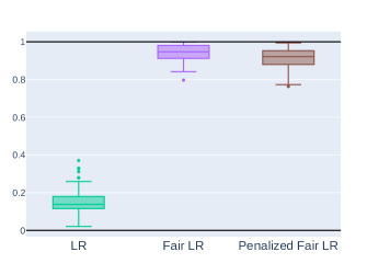
Figure 2. Disparate impact.

Given that we are now dealing with a different problem, we need to update the components that we will use in the iterative process. Then, we can rewrite our GLMM algorithm to ensure it can effectively handle this new problem. In the following, we will show in detail how to compute the components necessary for our algorithm extending the results of [39]. For $r\in[1,p]$ and for $l\in[1,l_{max}]$ with $l_{max}$ being the maximum number of iterations and the closed form for the pseudo Fisher matrix ($FP$)

$$FP_{r}(\delta^{(l)})=A_{r}W_{l}A_{r}+K\in\mathbb{R}^{(n+2)\times(n+2)},$$ (10)

with $A_{r}\mathrel{{\mathop{:}}{=}}[X_{r},Z]\in\mathbb{R}^{N\times(n+2)}$ , $K=Blockdiag(0,0,Q^{-1},\dots,Q^{-1})\leavevmode\nobreak\ \in\leavevmode\nobreak\ \mathbb{R}^{(n+2)\times(n+2)}$ being a block diagonal penalty matrix with diagonal of two zeros corresponding to intercept and the $r$-th fixed effect and $n$ times the matrix $Q^{-1}$, and

$$W_{l}=w(\delta^{(l-1)}),$$

with

$$w(\delta)=D(\delta)\Sigma^{-1}(\delta)D(\delta)^{\top}\in\mathbb{R}^{N\times N},$$

where D is the derivative of the inverse of the link function. In our case we use the logit function, then $h(\eta^{i})=g^{-1}(\eta^{i})=e^{\eta^{i}}/(1+e^{\eta^{i}})$, for $i\in[1,n]$ that is

$$\begin{split}D_{i}(\delta)&=\frac{\partial h(\eta^{i})}{\partial\eta}=\frac{e^{\eta^{i}}}{(1+e^{\eta^{i}})^{2}}=\Big{(}\frac{e^{\eta^{i}}}{1+e^{\eta^{i}}}\Big{)}\Big{(}1-\frac{e^{\eta^{i}}}{1+e^{\eta^{i}}}\Big{)}\\ &=h(\eta^{i})(1-h(\eta^{i})).\end{split}$$ (11)

Moreover, by [12],

$$\Sigma_{i}(\delta)=cov(y_{i}|\beta,b_{i})=h(\eta^{i})(1-h(\eta^{i}))\in\mathbb{R}^{T_{i}\times T_{i}}.$$ (12)

Combine (11) and (12) we obtained

$$D(\delta)=\Sigma(\delta),$$

being $D=diag(D_{1},\dots,D_{n})$, and then

$$w(\delta) =D(\delta)\Sigma^{-1}(\delta)D(\delta)^{\top}=D(\delta)D^{-1}(\delta)D(\delta)^{\top}$$

$$=D(\delta)^{\top}\in\mathbb{R}^{N\times N}.$$

For the score function for $r\in[1,p]$, we have the closed form obtained by differentiating the objective function (6)

$$s_{r}(\delta^{(l)})=A_{r}^{\top}W_{l}D_{l}^{-1}(y-\mu^{(l)})-K\delta_{r}^{(l)}\in\mathbb{R}^{(n+2)\times 1}$$ (13)

being $\mu^{(l)}=h(\eta^{(l)})\in\mathbb{R}^{N}$, $\delta_{r}^{\top}=(\beta_{0},\beta_{r},b^{\top})$ and $D_{l}=D(\delta^{(l-1)})$ that come by differentiating the inverse of the logit function.

For finding the best direction for the update we use the Bayesian Information Criterion $(BIC)\in\mathbb{R}^{p}$. The $BIC$ is a popular model selection criterion for GLMMs for being relatively easy to calculate, and it has been shown to perform well in a variety of simulations as can be seen in [40]:

$$BIC_{r}^{(l)}=-2\Gamma(\mu_{r}^{(l)})+2tr(H_{r}^{(l)})log(n),$$ (14)

with

$$\Gamma(\mu_{r}^{(l)})=\displaystyle\sum_{i=1}^{n}\displaystyle\sum_{t=1}^{T_{i}}y_{i_{t}}log(\mu_{i_{t}})-\mu_{i_{t}},$$

and

$$H_{r}^{(l)}=\displaystyle\sum_{k=0}^{l}M_{j_{k}}\displaystyle\prod_{i=0}^{k-1}(I-M_{j_{i}})\in\mathbb{R}^{N\times N},$$

being

$$M_{r}^{(l)}\mathrel{{\mathop{:}}{=}}\Sigma_{l}^{1/2}\tilde{H}_{r}^{(l)}\Sigma_{l}^{-1/2}\in\mathbb{R}^{N\times N},$$

being $\Sigma_{l}=\Sigma(\delta^{(l-1)})$, and

$$\tilde{H}_{r}^{(l)}=W_{l}^{1/2}A_{r}(A_{r}W_{l}A_{r}+K)^{-1}A_{r}^{\top}W_{l}^{1/2}\in\mathbb{R}^{N\times N}.$$

Now, as can be seen in [26] we can update the covariance matrix $Q^{(l)}$ by

$$Q^{(l)}=\frac{1}{n}\displaystyle\sum_{i=1}^{n}(V_{i}^{(l)}+b_{i}^{(l)}(b_{i}^{(l)})^{\top})\in\mathbb{R}.$$ (15)

In general, and in our case, the $V_{i}$ are computed via the formula

$$V_{i}=F_{i}^{-1}+F_{i}^{-1}\tilde{F}_{i}^{\top}(\hat{F}-\displaystyle\sum_{i=1}^{n}\tilde{F}_{i}F_{i}^{-1}\tilde{F}_{i}^{\top})^{-1}\tilde{F}_{i}F_{i}^{-1}\in\mathbb{R}$$

with

$$F_{i}=(Z^{i})^{\top}D_{i}(\delta)\Sigma_{i}(\delta)^{-1}D_{i}(\delta)Z^{i}+Q^{-1}\in\mathbb{R},$$

$$\tilde{F}_{i}=(X^{i})^{\top}D_{i}(\delta)\Sigma_{i}(\delta)^{-1}D_{i}(\delta)Z^{i}\in\mathbb{R}^{p},$$

and

$$\hat{F}=\displaystyle\sum_{i=1}^{n}(X^{i})^{\top}D_{i}(\delta)\Sigma_{i}(\delta)^{-1}D_{i}(\delta)X^{i}\in\mathbb{R}^{p\times p},$$

where $\hat{F}$, $\tilde{F}_{i}$ and $F_{i}$ are the elements of the pseudo Fisher matrix $FP(\delta)$ of the full model. For more detailed derivation see [25].

Given that we have a new objective function, we need to update the pseudo Fisher matrix and the score function. By the Equation (9), we have the penalization part being

$$\dfrac{\rho}{N}\|a^{\top}\delta\|^{2}_{2}.$$ (16)

As we can see in [24], we can substitute the pseudo Fisher matrix with the negative of the Hessian matrix ($\mathcal{H}$), i.e. $FP(\delta^{(l)})=-\mathcal{H}(\delta^{(l)})$. Hence,

$$\mathcal{H}(\dfrac{\rho}{N}\|a^{\top}\delta\|^{2}_{2})=\dfrac{\rho}{N}a^{\top}a.$$ (17)

than we can obtain the final Hessian $(\mathcal{FH})$ of the objective function (9) joining the Equations (10) and (17) and considering, w.l.o.g., $\rho=\dfrac{\rho}{N}$

$$\mathcal{FH}_{r}^{(l)}=FP_{r}(\delta^{(l-1)})-\rho a_{r}^{\top}a_{r}.$$

And the score function, that can be seen as the gradient $(\nabla)$, of the penalization part (16)

$$\nabla(\dfrac{\rho}{N}\|a^{\top}\delta\|^{2}_{2})=2\dfrac{\rho}{N}(a^{\top}a)\delta,$$ (18)

to obtain the final score function $(\mathcal{FS})$ of the objective function (9) we join the Equations (13) and (18) and considering, w.l.o.g., $\rho=2\dfrac{\rho}{N}$

$$\mathcal{FS}_{r}^{(l)}=s_{r}(\delta^{(l-1)})+\rho a_{r}^{\top}(a_{r}\delta^{(l-1)}_{r}).$$

Finally, we have all necessary components and motivations to propose an algorithm for solving the Fair Generalized Linear Mixed Model.

Algorithm 1 : Fair Generalized Linear Mixed Model

Given: $\mu^{(0)}$, $\beta_{0}^{(0)}$, $\beta^{(0)}$, $b^{(0)}$, $\eta^{(0)}$, $l_{max}$, $Q^{(0)}$.

Iteration:

(1) Refitting of residuals: For $l\in[1,l_{max}]$, (i) Computation of parameters For $r\in[1,p]$ the $r$-th Newton’s method step has the form:                             $\delta^{(l)}_{r}=(\mathcal{FH}_{r}^{(l-1)})^{-1}(\mathcal{FS}_{r}^{(l-1)})$ (ii) Selection step Select from $r\in[1,p]$ the index $j$ corresponding to the smallest $BIC_{r}^{(l)}$ and select the related $(\delta^{(l)}_{j})^{\top}=(\beta_{0}^{*},\beta_{j}^{*},(b^{*})^{\top})$. (iii) Update Set $\hskip 85.35826pt\beta^{(l)}_{0}=\beta^{(l-1)}_{0}+\beta^{*}_{0},$ and $\hskip 85.35826ptb^{(l)}=b^{(l-1)}+b^{*}$ and for $r\in[1,p]$ set                             $\beta_{r}^{(l)}=\begin{cases}\beta_{r}^{(l-1)}\hskip 42.67912pt\text{if }r\neq j\\ \beta_{r}^{(l-1)}+\beta_{r}^{*}\hskip 19.91684pt\text{if }r=j\end{cases}\,$ with $A\mathrel{{\mathop{:}}{=}}[X,Z]$ update $\hskip 85.35826pt\eta=A\delta^{(l)}$ (2) Computing of variance-covariance components:                                 $Q^{(l)}=\dfrac{1}{n}\displaystyle\sum_{i=1}^{n}(V_{i}^{(l)}+b_{i}^{(l)}(b_{i}^{(l)})^{\top}).$

until $Q^{(l)}=Q^{(l-1)}$.

2.5. Cluster-Regularized Logistic Regression

In the numerical tests (3.3) and (3.4), a weakness in the Fair GLMM algorithm was observed. When the data did not have random effects, accuracy was worse than in simple logistic regression. This is due to the fact that in the mixed model formulation, if $b_{i}=0$ $\forall$ $i\in[1,n]$, it would imply that $\sigma^{2}_{b}=0$ this is on the boundary of the parameter space, and hence it imposes difficulties when estimating the Variance-Covariance matrix via maximum likelihood. It is noteworthy that this would be irrelevant to the optimization problem itself because the solver employs algorithms that do not rely on the Variance-Covariance matrix.

For this reason, we propose the following optimization model that will deal with this issue using a L2 regularization ([20]).

$$\displaystyle\min_{\beta,b}\hskip 2.84544pt -\displaystyle\sum_{i=1}^{n}\displaystyle\sum_{j=1}^{T_{i}}[y_{i_{j}}\log(m_{\beta,b}(x^{i_{j}}))+(1-y_{i_{j}})\log(1-m_{\beta,b}(x^{i_{j}}))]+\lambda\sum_{i=1}^{n}b_{i}^{2}$$ (19)

s.t. $$\frac{1}{N}\displaystyle\sum_{i=1}^{n}\displaystyle\sum_{j=1}^{T_{i}}(s_{i_{j}}-\bar{s})(\beta^{\top}x^{i_{j}}+b_{i})\leq c$$ (20)

$$\frac{1}{N}\displaystyle\sum_{i=1}^{n}\displaystyle\sum_{j=1}^{T_{i}}(s_{i_{j}}-\bar{s})(\beta^{\top}x^{i_{j}}+b_{i})\geq-c$$ (21)

with

$$m_{\beta,b}(x^{i_{j}})=\dfrac{1}{1+e^{-(\beta^{\top}x^{i_{j}}+b_{i})}},$$

$\bar{s}$ from Equation (5) and $\lambda\sum_{i}^{n}b_{i}^{2}$ from [15]. We will denote Problem (19) as Cluster-Regularized Logistic Regression (CRLR) and problem (19) - (21) as Fair Cluster-Regularized Logistic Regression (Fair CRLR).

3. Simulation Study

In this section, we aim to present numerical tests to demonstrate the effectiveness of the proposed method.

First we present the step-by-step strategy used to create the datasets and to conduct the numerical experiments. Using the Julia 1.9 ([8]) language with the packages Distributions ([7]), GLM ([4]), MixedModels ([3]), DataFrames ([11]), MLJ ([9]) and MKL ([19]), we generate the following parameters:

• Number of points: Number of points in the dataset;

• $\beta^{\prime}s$: The fixed effects;

• $b^{\prime}s$: The random effects with distribution $N(0,Q)$, with covariance matrix $Q$ (Used only when indicated);

• Data points: The covariate vector associated with fixed effects with distribution $N(0,1)$;

• $c$: Threshold from Fair Logistic Regression;

• $\rho$: Lagrange multiplier;

• seed: Random seed used in the generation of data;

• Train-Test split: Approximately 0.4% of the dataset was used for the training set, and 99.6% for the test set. This percentage was due to the fact that we randomly selected 3 to 5 points from each strata for the training set.

The predictions of the synthetic dataset were computed using

$$m=\dfrac{1}{1+e^{-(\beta^{T}x+b)}}$$ (22)

in tests where the dataset has random effects, and

$$m=\dfrac{1}{1+e^{-\beta^{T}x}}$$ (23)

in tests where the dataset has just fixed effects. Finally,

$$y=Binomial(1,m).$$

The comparisons will be made by comparing the accuracy and the disparate impact between the Algorithms:

1. Generalized linear mixed model (GLMM);

2. Fair generalized linear mixed model (Fair GLMM);

3. Cluster-Regularized Logistic Regression (CRLR);

4. Fair Cluster-Regularized Logistic Regression (Fair CRLR),

5. Logistic Regression (LR);

6. Fair Logistic Regression (Fair LR).

The test were conducted on a laptop with an Intel Core i9-13900HX processor with a clock speed of 5.40 GHz, 64 GB of RAM, and Windows 11 operating system, with 64-bit architecture.

To compute accuracy, first we need to compute the predictions using Equations (22) and (23) with,

$$\hat{y}=\begin{cases}1\hskip 11.38092pt\text{if }\hskip 1.42271ptm\geq 0.5\\ 0\hskip 11.38092pt\text{if }\hskip 1.42271ptm<0.5\end{cases}\,.$$ (24)

Given the true label of all points, we can distinguish them into four categories: true positive (TP) or true negative (TN) if the point is classified correctly in the positive or negative class, respectively, and false positive (FP) or false negative (FN) if the point is misclassified in the positive or negative class, respectively. Based on this, we can compute the accuracy, where a higher value indicates a better classification, as follows,

$$AC=\dfrac{TP+TN}{TP+TN+FP+FN}\in[0,1].$$

To compute the disparate impact of a specific sensitive feature $s$ we use the following equation as can be seen in [36],

$$DI=\dfrac{p(\hat{y}|s=1)}{p(\hat{y}|s=0)}\in[0,1].$$

Disparate impact, as a measure, should be equal to 1. This indicates that discrimination does not exist. Values greater or lower than 1 suggest that unwanted discrimination exists. However, $DI=2$ and $DI=0.5$ represent the same level of discrimination, although in the first case, the difference between the perfect value is 1, and in the latter case, it is 0.5. To avoid such situations, we use the minimum of $DI$ and its inverse.

$$DI=\min\Big{(}\dfrac{p(\hat{y}|s=1)}{p(\hat{y}|s=0)},\dfrac{p(\hat{y}|s=0)}{p(\hat{y}|s=1)}\Big{)}\in[0,1].$$

In the following, we generate four different synthetic populations (scenarios) to compare the competing algorithms. For each synthetic data set 100 samples are drawn. The simulation results are discussed for each synthetic data set using 2 images that represent, respectively, the accuracy and the disparate impact.

All figures were created using the Plots and PlotlyJS packages, developed by [18] and all hyperparameters were selected via cross-validation ([14]).

Across all of our tests, the initial parameters were:

• $\beta_{0}^{(0)}=1.0$;

• $\beta^{(0)}=0\in{\mathbb{R}}^{p}$;

• $b^{(0)}$: MixedModel function from GLM package;

• $\mu^{(0)}:$ MixedModel function from GLM package;

• $\eta^{(0)}:$ MixedModel function from GLM package;

• $Q^{(0)}=2.0$.

3.1. Unfair population with strata effect

Parameters of data generation:

• $\beta$’s $=[-2.0,0.4,0.8,0.5,3.0]$;

• $b$’s: 100 stratas with $b_{i}\sim N(0,3.0)$, with $i\in[1,100]$;

• $c=0.1$;

• $\rho=0.8$;

• $\lambda=1$.

Algorithm	Mean	p25	Median	p75	p90	std
GLMM	0.89	0.89	0.90	0.91	0.92	0.02
Fair GLMM	0.85	0.82	0.87	0.90	0.91	0.07
CRLR	0.81	0.80	0.81	0.82	0.83	0.01
Fair CRLR	0.81	0.80	0.81	0.82	0.83	0.02
LR	0.71	0.71	0.71	0.71	0.71	0.01
Fair LR	0.66	0.66	0.66	0.67	0.67	0.01

Table 1. Accuracy.

Algorithm	Mean	p25	Median	p75	p90	std
GLMM	0.35	0.31	0.34	0.39	0.43	0.10
Fair GLMM	0.58	0.40	0.53	0.75	0.89	0.21
CRLR	0.07	0.04	0.07	0.09	0.12	0.03
Fair CRLR	0.55	0.50	0.54	0.59	0.62	0.06
LR	0.02	0.01	0.02	0.04	0.06	0.03
Fair LR	0.37	0.29	0.38	0.44	0.51	0.11

Table 2. Disparate impact

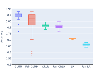
Figure 3. Accuracy.

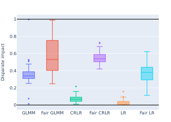
Figure 4. Disparate impact.

The results in Table 1 and Figure 3 demonstrate superior accuracy for GLMM, Fair GLMM, CRLR, and Fair CRLR in this experiment set. This is unsurprising, as logistic regression doesn’t account for random effects. We can also see that the GLMM performs better on both metrics compared to the optimization problems.

Table 2 and Figure 4 show that we also obtained an improvement in the disparate impact on the Fair algorithms. Note that make sense since we have a unfair population.

3.2. Fair population with strata effect

Parameters of data generation:

• $\beta$’s $=[-0.1,1,2,1,0.1]$;

• $b$’s: 100 stratas with $b_{i}\sim N(0,3.0)$, with $i\in[1,100]$;

• $c=0.1$;

• $\rho=0.8$;

• $\lambda=1$.

Algorithm	Mean	p25	Median	p75	p90	std
GLMM	0.82	0.78	0.85	0.89	0.90	0.09
Fair GLMM	0.84	0.80	0.86	0.89	0.91	0.07
CRLR	0.83	0.82	0.83	0.83	0.84	0.01
Fair CRLR	0.83	0.82	0.83	0.83	0.84	0.01
LR	0.75	0.74	0.75	0.75	0.75	0.01
Fair LR	0.75	0.74	0.75	0.75	0.75	0.01

Table 3. Accuracy.

Algorithm	Mean	p25	Median	p75	p90	std
GLMM	0.95	0.94	0.97	0.99	0.99	0.08
Fair GLMM	0.93	0.90	0.95	0.98	0.99	0.08
CRLR	0.94	0.91	0.95	0.98	0.99	0.04
Fair CRLR	0.95	0.92	0.96	0.98	0.99	0.04
LR	0.93	0.90	0.94	0.97	0.99	0.05
Fair LR	0.94	0.91	0.95	0.97	0.99	0.04

Table 4. Disparate impact

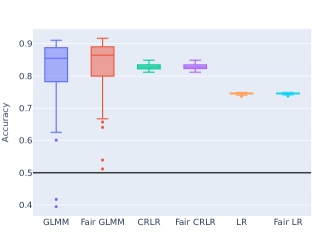
Figure 5. Accuracy.

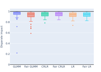
Figure 6. Disparate impact.

As can be seen in Table 3 and in the Figure 5, in this set of experiments, we obtained a better accuracy in GLMM, Fair GLMM, CRLR and Fair CRLR. This is expected since logistic regression does not account for random effects.

Table 4 and Figure 6 show that the disparate impact remains almost the same in all tests since we have a fair population.

3.3. Unfair population without strata effect

Parameters of data generation:

• $\beta$’s $=[-0.8,0.4,0.8,0.5,1.8]$;

• $c=0.1$;

• $\rho=0.8$;

• $\lambda=1$.

Algorithm	Mean	p25	Median	p75	p90	std
GLMM	0.63	0.62	0.63	0.64	0.65	0.02
Fair GLMM	0.62	0.61	0.62	0.63	0.64	0.03
CRLR	0.78	0.78	0.78	0.78	0.79	0.01
Fair CRLR	0.68	0.67	0.68	0.69	0.69	0.01
LR	0.70	0.70	0.70	0.70	0.70	0.01
Fair LR	0.69	0.68	0.69	0.69	0.69	0.01

Table 5. Accuracy.

Algorithm	Mean	p25	Median	p75	p90	std
GLMM	0.36	0.29	0.36	0.42	0.48	0.11
Fair GLMM	0.69	0.48	0.71	0.89	0.97	0.22
CRLR	0.04	0.02	0.04	0.06	0.08	0.02
Fair CRLR	0.56	0.51	0.55	0.60	0.66	0.07
LR	0.18	0.12	0.17	0.22	0.29	0.08
Fair LR	0.54	0.48	0.53	0.60	0.67	0.10

Table 6. Disparate impact

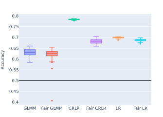
Figure 7. Accuracy.

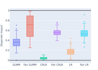
Figure 8. Disparate impact.

Our experiments, detailed in Table 5 and Figure 7, show a slight decrease in accuracy for GLMM algorithms. This is likely because GLMMs attempt to account for random effects, even when they are absent. This additional parameter estimation in GLMMs can lead to a reduction in accuracy compared to logistic regression optimization problems.

Table 6 and Figure 8 show that we obtained an improvement in the disparate impact on the Fair algorithms. Note that make sense since we have a unfair population.

3.4. Fair population without strata effect

Parameters of data generation:

• $\beta$’s $=[-0.1,1,2,1,0.1]$;

• $c=0.1$;

• $\rho=0.8$;

• $\lambda=1$.

Algorithm	Mean	p25	Median	p75	p90	std
GLMM	0.71	0.71	0.73	0.74	0.75	0.06
Fair GLMM	0.70	0.70	0.73	0.74	0.75	0.07
CRLR	0.82	0.82	0.82	0.82	0.83	0.01
Fair CRLR	0.82	0.82	0.82	0.82	0.83	0.01
LR	0.82	0.82	0.83	0.83	0.83	0.01
Fair LR	0.83	0.82	0.83	0.83	0.83	0.01

Table 7. Accuracy.

Algorithm	Mean	p25	Median	p75	p90	std
GLMM	0.89	0.86	0.92	0.96	0.98	0.12
Fair GLMM	0.88	0.86	0.93	0.97	0.99	0.15
CRLR	0.92	0.89	0.93	0.97	0.99	0.06
Fair CRLR	0.94	0.91	0.95	0.98	0.99	0.05
LR	0.92	0.88	0.93	0.97	0.99	0.06
Fair LR	0.94	0.91	0.95	0.98	0.99	0.05

Table 8. Disparate impact

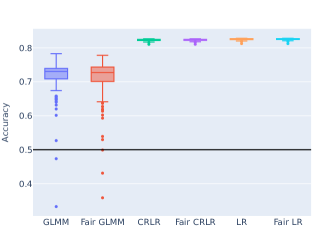
Figure 9. Accuracy.

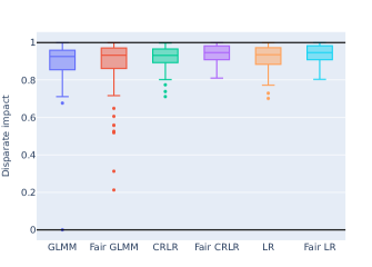
Figure 10. Disparate impact.

Our experiments, detailed in Table 7 and Figure 9, show a decrease in accuracy for GLMM algorithms for the same reason from Scenario 3.3.

Table 8 and Figure 10 show that we also have a very similar disparate impact in all algorithms. Note that make sense since we have a fair population.

4. Application

In this set of experiments, we will test the Bank marketing dataset, which has a strata bias related to the duration of telephone calls, the longer the call duration, (calls with longer duration imply a higher probability of the label being $1$), and a sensitive feature, which in this case is housing loan, the housing loan feature can be considered a sensitive feature because it is directly linked to injustice in its generation, as can be seen in [13] and in [29]. The data is related to direct marketing campaigns of a Portuguese banking institution. The marketing campaigns were based on phone calls. Often, more than one contact was required with the same client, in order to determine if the product (bank term deposit) would be subscribed ($y=1$) or not ($y=0$). Were conducted 100 samples with 3.5% of the data as the training set and the remaining data as the test set. Since the application under study employs random effects, we will conduct the comparisons using solely GLMM and logistic regression.

The features used in the prediction process are the follows:

• Age

• Job

• Marital status

• Education

• Has credit in default?

• Has housing loan?

• Has personal loan?

• Contact communication type

• Last contact month of year

• Last contact day of the week

• Number of contacts performed during this campaign and for this client

• Number of days that passed by after the client was last contacted from a previous campaign

• Number of contacts performed before this campaign and for this client

• Outcome of the previous marketing campaign

• Employment variation rate

• Consumer price index

• Consumer confidence index

• Euribor 3 month rate

• Number of employees

Algorithm	Mean	p25	Median	p75	p90	std
GLMM	0.69	0.68	0.70	0.70	0.71	0.01
Fair GLMM	0.68	0.68	0.69	0.70	0.70	0.01
LR	0.57	0.56	0.57	0.58	0.59	0.02
Fair LR	0.53	0.52	0.53	0.54	0.56	0.02

Table 9. Accuracy

Algorithm	Mean	p25	Median	p75	p90	std
GLMM	0.73	0.66	0.72	0.79	0.86	0.10
Fair GLMM	0.87	0.81	0.90	0.95	0.98	0.10
LR	0.35	0.22	0.34	0.45	0.54	0.15
Fair LR	0.82	0.78	0.88	0.94	0.98	0.19

Table 10. Disparate Impact

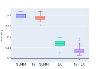
Figure 11. Accuracy.

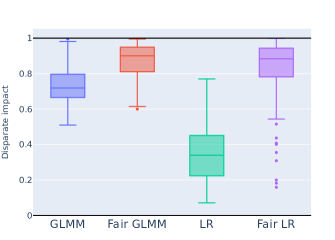
Figure 12. Disparate Impact.

As can be seen in Table 9 and in the Figure 11, in this set of experiments, we obtained a better accuracy in GLMM and Fair GLMM. This result aligns with the random effects structure of the data.

Table 10 and Figure 12 show that we also obtained an improvement in the disparate impact on the Fair algorithms. Note that make sense since we have a unfair population.

4.1. Sensitivity analysis

The Lagrange multiplier strategy, using Karush-Kuhn-Tucker (KKT) conditions, is a powerful tool for analyzing the sensitivity of constrained optimization problems. To perform the sensitivity analysis of the constraints of problems, we will use the strategy, described in Appendix A.

As seen in Section 2.3 fairness constraints operate within an interval $[-c,c]$. However, we will set $c=0$. Because this value in the constraint makes the optimization problem as fair as possible, and then, we can say that if we do not obtain a large perturbation in the objective function with $c=0$, the constraint is useless for the problem. This is because, with other values of $c$, the perturbation would be even smaller.

The sensitivity analysis (SA) or, as it is also known, Lagrange multipliers of fair logistic regression problems is important for understanding how the fairness constraints affect the model’s predictions. By analyzing the sensitivity of the model’s predictions to changes in the fairness constraints, we can identify which constraints, among the constraints of sensitive features, are most important for achieving fairness. We can also refer to this value as the shadow price, in essence, the shadow price reflects the economic value of relaxing or tightening a constraint in an optimization problem. It represents the marginal impact on the objective function of making a small adjustment to a constraint, that is if the shadow price is $P$, it means that the value of the objective function will increase by $P$ if the constraint is relaxed as we can see in [37].

In this application, we consider Marital Status, Education, and Housing Loan as sensitive features. The values below refer to the Lagrange multiplier values and the disparate impact values found in the $100$ tests performed on this application. The disparate impact improvement are compared to the regular logistic regression and the accuracy drop are compared with the regular GLMM.

Sensitivity Feature	SA	DI improve	AC drop
Housing	28.7	134.3%	7.5%
Marital Status	11.9	14.4%	$<$ 1.0%
Education	12.5	16.6%	$<$ 1.0%
Marital Status/Education	13.5/14.7	13.9%/18.5%	$<$ 1.0%
Housing/Marital Status	30.9/14.4	86.5%/9.8%	7.9%
Housing/Education	29.3/13.8	82.5%/16.0%	7.9%

Table 11. Sensitivity analysis table.

As we can see in Table 11, the sensitive feature constraint that made the biggest difference in the objective function and, therefore, achieved a greater improvement in the Disparate Impact was the housing feature.

We can also note, that in this application simply accounting for the random effect without adding fairness constraints already significantly improves the disparate impact. As expected, adding the fairness constraints, yields even better disparate impact.

5. Conclusion

In this work, we proposed an algorithm for a fair generalized linear mixed model (GLMM) and a optimization model (CRLR) that allows for controlling the disparate impact of a sensitive feature. This way, a fair prediction can be achieved even when the data has an inherent grouping structure. To our knowledge, this has not been proposed before.

We leverage simulations to showcase how our approach overcomes limitations in existing methods. It delivers superior results when group structures significantly impact prediction accuracy or fairness. We also concluded when to use which approach, considering that if we have the information about random effects, the Fair GLMM performs better, otherwise the optimization model is also a good choice.

Furthermore, we applied our method to the Bank marketing dataset. Here, it effectively addressed random effects while mitigating disparate impact associated with the sensitive feature.

Additionally, we explore how KKT conditions can be used to assess feature sensitivity in fair logistic regression. This analysis helps identify the specific sensitive variable whose disparate impact we aimed to mitigate in the process.

To enhance the framework’s capabilities, future work could focus on incorporating additional fairness constraint options within the GLMM. Additionally, efforts to optimize the computational efficiency of the proposed algorithms would be beneficial.

Appendix A Sensitivity analysis

The generalization of the sensitivity analysis to multiple sensitive features is straightforward. We simply add a Lagrange multiplier for each sensitive feature. The sensitivity of the objective function can then be determined by the corresponding Lagrange multipliers $\zeta$. Each $\zeta_{k}$ is the perturbation of the k-th sensitive feature, with $k=1,...,K$, where $K$ is the number of sensitive features that we want to use in the tests. And for each sensitive feature, we must use the corresponding $s^{k}$ and $\bar{s^{k}}$.

The sensitivity analysis of fair logistic regression problems is important for understanding how the fairness constraints affect the model’s predictions. By analyzing the sensitivity of the model’s predictions to changes in the fairness constraints, we can identify which constraints are most important for achieving fairness.

The calculation of the sensitivity analysis equations for fair logistic regression problems, fixing $c=0$, is done using the following optimization problem for a fixed $k\in[1,K]$:

$$\begin{split}\displaystyle\min_{\beta}\hskip 2.84544pt&-\displaystyle\sum_{\ell=1}^{N}[y_{\ell}\log(m_{\beta}(x^{\ell}))+(1-y_{\ell})\log(1-m_{\beta}(x^{\ell}))]\\ \textrm{s.t.}\hskip 2.84544pt&\frac{1}{N}\displaystyle\sum_{\ell=1}^{N}\displaystyle(s_{\ell}^{k}-\bar{s^{k}})(\beta^{\top}x^{\ell})=0\end{split}$$ (25)

with $m_{\beta}(x^{\ell})$

$$m_{\beta}(x^{\ell})=\dfrac{1}{1+e^{-(\beta^{\top}x^{\ell})}}.$$

Calculating the Lagrangian for problem $\eqref{ret11111}$, we achieve:

$$\mathcal{L}(\beta,\zeta_{k})=-\sum_{\ell=1}^{N}\Big{[}y_{\ell}\log(m_{\beta}(x^{\ell}))+(1-y_{\ell})\log(1-m_{\beta}(x^{\ell}))\Big{]}+\zeta_{k}\Big{(}\frac{1}{N}\sum_{\ell=1}^{N}(s_{\ell}^{k}-\bar{s^{k}})(\beta^{\top}x^{\ell})\Big{)}$$

Now, calculating the partial derivative of the Lagrangian with respect to $\beta$ as can be see in [28], we have:

$$\nabla\mathcal{L}(\beta,\zeta_{k})=-\sum_{\ell=1}^{N}\Big{(}m_{\beta}(x^{\ell})-y_{\ell}\Big{)}x^{\ell}+\zeta_{k}\Big{(}\sum_{\ell=1}^{N}(s_{\ell}^{k}-\bar{s^{k}})(x^{\ell})\Big{)}$$

Using the Karush-Kuhn-Tucker (KKT) conditions, as we can see in [6], we find $\nabla\mathcal{L}(\beta,\zeta_{k})=0$, so:

$$-\sum_{\ell=1}^{N}\Big{(}\dfrac{1}{1+e^{-(\beta^{\top}x^{\ell})}}-y_{\ell}\Big{)}x^{\ell}+\zeta_{k}\Big{(}\sum_{\ell=1}^{N}(s_{\ell}^{k}-\bar{s^{k}})(x^{\ell})\Big{)}=0$$ (26)

Since we already have the fixed effects $\beta$’s, the perturbations of all constraints can be obtained by solving the system (26). Since the solution found by solving the optimization problem is an optimal point, the KKT conditions are satisfied, so the system has a guaranteed solution.

For the Cluster-Regularized Logistic Regression, fixing $c=0$, the sensitivity analysis is done using the following optimization problem for a fixed $k\in[1,K]$:

$$\begin{split}\displaystyle\min_{\beta,b}\hskip 2.84544pt&-\displaystyle\sum_{i=1}^{n}\displaystyle\sum_{j=1}^{T_{i}}[y_{i_{j}}\log(m_{\beta,b}(x^{i_{j}}))+(1-y_{i_{j}})\log(1-m_{\beta,b}(x^{i_{j}}))]+\lambda\sum_{i}^{n}b_{i}^{2}\\ \textrm{s.t.}\hskip 2.84544pt&\frac{1}{N}\displaystyle\sum_{i=1}^{n}\displaystyle\sum_{j=1}^{T_{i}}(s_{i_{j}}^{k}-\bar{s^{k}})(\beta^{\top}x^{i_{j}}+b_{i})=0\end{split}$$ (27)

with

$$m_{\beta,b}(x^{i_{j}})=\dfrac{1}{1+e^{-(\beta^{\top}x^{i_{j}}+b_{i})}},$$

calculating the Lagrangian for problem $\eqref{ret1231111}$, we achieve:

$$\begin{split}\mathcal{L}(\beta,b,\zeta_{k})&=-\displaystyle\sum_{i=1}^{n}\displaystyle\sum_{j=1}^{T_{i}}[y_{i_{j}}\log(m_{\beta,b}(x^{i_{j}}))+(1-y_{i_{j}})\log(1-m_{\beta,b}(x^{i_{j}}))]\\ &+\lambda\sum_{i=1}^{n}b_{i}^{2}+\zeta_{k}\Big{(}\frac{1}{N}\displaystyle\sum_{i=1}^{n}\displaystyle\sum_{j=1}^{T_{i}}(s_{i_{j}}^{k}-\bar{s^{k}})(\beta^{\top}x^{i_{j}}+b_{i})\Big{)}\end{split}$$ (28)

Now, computing the partial derivative of the Lagrangian with respect to $\beta$, we have:

$$\begin{split}\nabla_{\beta}\mathcal{L}(\beta,b,\zeta_{k})&=-\displaystyle\sum_{i=1}^{n}\displaystyle\sum_{j=1}^{T_{i}}\Big{[}y_{i_{j}}\Big{(}\frac{x^{i_{j}}}{1+e^{(\beta^{\top}x^{i_{j}}+b_{i})}}\Big{)}-(1-y_{i_{j}})\Big{(}\frac{x^{i_{j}}}{1+e^{-(\beta^{\top}x^{i_{j}}+b_{i})}}\Big{)}\Big{]}\\ &+\zeta_{k}(\frac{1}{N}\displaystyle\sum_{i=1}^{n}\displaystyle\sum_{j=1}^{T_{i}}(s_{i_{j}}^{k}-\bar{s^{k}})x^{i_{j}})\end{split}$$ (29)

and the partial derivative with respect to each $b_{i}$:

$$\begin{split}\nabla_{b_{i}}\mathcal{L}(\beta,b,\zeta_{k})&=-\displaystyle\sum_{j=1}^{T_{i}}\Big{[}y_{i_{j}}\Big{(}\frac{1}{1+e^{(\beta^{\top}x^{i_{j}}+b_{i})}}\Big{)}-(1-y_{i_{j}})\Big{(}\frac{1}{1+e^{-(\beta^{\top}x^{i_{j}}+b_{i})}}\Big{)}\Big{]}\\ &+2\lambda b_{i}+\zeta_{k}(\frac{1}{N}\displaystyle\sum_{j=1}^{T_{i}}(s_{i_{j}}^{k}-\bar{s^{k}}))\end{split}$$ (30)

that is,

$$\nabla\mathcal{L}(\beta,b,\zeta_{k})=\begin{bmatrix}\nabla_{\beta}\mathcal{L}(\beta,b,\zeta_{k})\\ \nabla_{b}\mathcal{L}(\beta,b,\zeta_{k})\\ \end{bmatrix}=\begin{bmatrix}\nabla_{\beta}\mathcal{L}(\beta,b,\zeta_{k})\\ \nabla_{b_{1}}\mathcal{L}(\beta,b_{1},\zeta_{k})\\ \vdots\\ \nabla_{b_{i}}\mathcal{L}(\beta,b_{i},\zeta_{k})\\ \end{bmatrix}.$$

Using the Karush-Kuhn-Tucker (KKT) conditions, we find $\nabla\mathcal{L}(\beta,b,\zeta_{k})=0$ and since we already have the fixed effects $\beta$’s and the random effects $b$’s, the Lagrange multipliers of all constraints can be obtained by solving the system. Since the solution found by solving the optimization problem (19) - (21) is an optimal point, the KKT conditions are satisfied and the system has a guaranteed solution.

References

- [1] S Aghaei, M J Azizi and P Vayanos “Learning optimal and fair decision trees for non-discriminative decision-making” In Proceedings of the AAAI conference on artificial intelligence 33.01, 2019, pp. 1418–1426
- [2] S Barocas and A D Selbst “Big data’s disparate impact” In Calif. L. Rev. 104 HeinOnline, 2016, pp. 671
- [3] D Bates et al. “JuliaStats/MixedModels.jl: v4.22.2” Zenodo, 2023 DOI: 10.5281/zenodo.10069987
- [4] D Bates et al. “JuliaStats/GLM.jl: v1.8.0” Zenodo, 2022 DOI: 10.5281/zenodo.6580436
- [5] R Berk et al. “A convex framework for fair regression” In arXiv preprint arXiv:1706.02409, 2017
- [6] D P Bertsekas, A Nedic and A Ozdaglar “Convex analysis and optimization” Nashua: Athena Scientific, 2003
- [7] M Besançon et al. “Distributions.jl: Definition and Modeling of Probability Distributions in the JuliaStats Ecosystem” In Journal of Statistical Software 98.16, 2021, pp. 1–30 DOI: 10.18637/jss.v098.i16
- [8] J Bezanson, A Edelman, S Karpinski and V B Shah “Julia: A fresh approach to numerical computing” In SIAM review 59.1, 2017, pp. 65–98 DOI: 10.1137/14100067
- [9] A Blaom, F Kiraly, T Lienart and S Vollmer “alan-turing-institute/MLJ.jl: v0.5.3” Zenodo, 2019 DOI: 10.5281/zenodo.3541506
- [10] R Bono, R Alarcón and M J Blanca “Report Quality of Generalized Linear Mixed Models in Psychology: A Systematic Review” In Frontiers in Psychology 12, 2021 DOI: 10.3389/fpsyg.2021.666182
- [11] M Bouchet-Valat and B Kamiński “DataFrames.jl: Flexible and Fast Tabular Data in Julia” In Journal of Statistical Software 107.4, 2023, pp. 1–32 DOI: 10.18637/jss.v107.i04
- [12] N E Breslow and D G Clayton “Approximate Inference in Generalized Linear Mixed Models” In Journal of the American Statistical Association 88.421 [American Statistical Association, Taylor & Francis, Ltd.], 1993, pp. 9–25
- [13] E Brooke “Fair Housing Trends Report” Accessed: 2023-11-13, https://nationalfairhousing.org/resource/2023-fair-housing-trends-report/, 2023
- [14] M W Browne “Cross-validation methods” In Journal of mathematical psychology 44.1 Elsevier, 2000, pp. 108–132
- [15] J P Burgard and J V Pamplona “Fair Mixed Effects Support Vector Machine”, 2024 arXiv:2405.06433 [cs.LG]
- [16] M Casals, M Girabent-Farrés and J L Carrasco “Methodological Quality and Reporting of Generalized Linear Mixed Models in Clinical Medicine (2000–2012): A Systematic Review” In PLoS ONE 9, 2014
- [17] S Caton and C Haas “Fairness in machine learning: A survey” In ACM Computing Surveys ACM New York, NY, 2020
- [18] S Christ et al. “Plots.jl – a user extendable plotting API for the julia programming language” Journal of Open Research Software, 2023 DOI: https://doi.org/10.5334/jors.431
- [19] Intel Corporation “Intel Math Kernel Library” Intel Corporation, 2023
- [20] C Cortes, M Mohri and A Rostamizadeh “L2 regularization for learning kernels” In arXiv preprint arXiv:1205.2653, 2012
- [21] S Das et al. “Fairness measures for machine learning in finance” In The Journal of Financial Data Science Institutional Investor Journals Umbrella, 2021
- [22] H Do et al. “Fair generalized linear models with a convex penalty” In International Conference on Machine Learning, 2022, pp. 5286–5308 PMLR
- [23] B Green “Fair” risk assessments: A precarious approach for criminal justice reform” In 5th Workshop on fairness, accountability, and transparency in machine learning, 2018, pp. 1–5
- [24] P J Green and B W Silverman “Nonparametric Regression and Generalized Linear Models: A roughness penalty approach”, Chapman & Hall/CRC Monographs on Statistics & Applied Probability Florida: CRC Press, 1993
- [25] Q Gu, Z Li and J Han “Generalized fisher score for feature selection” In arXiv preprint arXiv:1202.3725, 2012
- [26] D A Harville “Maximum likelihood approaches to variance component estimation and to related problems” In Journal of the American statistical association 72.358 Virgínia: Taylor & Francis, 1977, pp. 320–338
- [27] D A Hensher and W H Greene “The mixed logit model: the state of practice” In Transportation 30 New York: Springer, 2003, pp. 133–176
- [28] J M Hilbe “Logistic regression models” Florida: CRC press, 2009
- [29] B Howell “Exploiting Race and Space: Concentrated Subprime Lending as Housing Discrimination” In California Law Review 94.1 California Law Review, Inc., 2006, pp. 101–147
- [30] K Lange “Newton’s Method and Scoring” In Mathematical and Statistical Methods for Genetic Analysis New York, NY: Springer New York, 2002, pp. 39–58 DOI: 10.1007/978-0-387-21750-5_3
- [31] Sharon L Lohr “Sampling : Design and Analysis” Florence, KY: Brooks/Cole, 2009
- [32] S Moro, P Rita and P Cortez “Bank Marketing” DOI: https://doi.org/10.24432/C5K306, UCI Machine Learning Repository, 2012
- [33] D J Neter, M H Kutner and C J Nachtsheim “MP Applied Linear Regression Models-Revised Edition with Student CD” Dubuque: McGraw-Hill Education, 2004
- [34] J Nocedal “Penalty and Augmented Lagrangian Methods” In Numerical Optimization New York: Springer New York, 2006, pp. 497–528
- [35] M Olfat and A Aswani “Spectral algorithms for computing fair support vector machines” In International conference on artificial intelligence and statistics, 2018, pp. 1933–1942 PMLR
- [36] S Radovanović, A Petrović, B Delibašić and M Suknović “Enforcing fairness in logistic regression algorithm” In 2020 International Conference on INnovations in Intelligent SysTems and Applications (INISTA), 2020, pp. 1–7 DOI: 10.1109/INISTA49547.2020.9194676
- [37] A Smith “Shadow price calculations in distorted economies” In The Scandinavian Journal of Economics JSTOR, 1987, pp. 287–302
- [38] W W Stroup “Generalized Linear Mixed Models: Modern Concepts, Methods and Applications”, Chapman & Hall/CRC Texts in Statistical Science Oxfordshire: Taylor & Francis, 2012
- [39] G Tutz and A Groll “Generalized linear mixed models based on boosting” In Statistical Modelling and Regression Structures: Festschrift in Honour of Ludwig Fahrmeir Springer, 2010, pp. 197–215
- [40] S I Vrieze “Model selection and psychological theory: a discussion of the differences between the Akaike information criterion (AIC) and the Bayesian information criterion (BIC).” In Psychological methods 17.2 American Psychological Association, 2012, pp. 228
- [41] M Zafar, I Valera, M Rodriguez and K P Gummadi “Fairness Constraints: A Mechanism for Fair Classification”, 2015
- [42] M B Zafar, I Valera, M Gomez-Rodriguez and K P Gummadi “Fairness Constraints: A Flexible Approach for Fair Classification” In Journal of Machine Learning Research 20.75, 2019, pp. 1–42
- [43] W Zhang et al. “Farf: A fair and adaptive random forests classifier” In Pacific-Asia conference on knowledge discovery and data mining, 2021, pp. 245–256 Springer