1. Introduction

Consider the fourth order nonlinear Schrödinger equation (4NLS)

$$iu_{t}+u_{xx}-u_{xxxx}+|u|^{\alpha}u=0,$$ (1.1)

where $u:\mathbb{R}\times\mathbb{R}\rightarrow\mathbb{C}$ and $\alpha>0$. Since $u$ is a complex function, we sometimes write $u=u_{1}+iu_{2}\equiv(u_{1},u_{2})$ in order to simplify the notation. The physical motivation concerning particular cases of the equation $(\ref{NLS-equation})$ was introduced in [15] and [16]. In fact, when $\alpha=2$, it is related to the propagation of intense laser beams in a bulk medium with Kerr nonlinearity when small fourth-order dispersion is taken into account. Moreover, equation $(\ref{NLS-equation})$ has been considered in connection with nonlinear fiber optics and the theory of optical solitons in gyrotropic media. An interesting fact arises when we examine equation $(\ref{NLS-equation})$ from a mathematical standpoint, as it does not enjoy scaling invariance due to the presence of the mixed dispersion term. This property is very important for the standard nonlinear Schrödinger equation (NLS),

$$iu_{t}+u_{xx}+|u|^{\alpha}u=0.$$ (1.2)

Let $\lambda>0$ be fixed. The scaling invariance $u\mapsto\lambda^{\frac{2}{\alpha}}u(\lambda x,\lambda^{2}t)$ applied to the equation $(\ref{2NLS-equation})$ is useful, for instance, to know the connection between the existence of global solutions in $\mathbb{H}^{1}=H^{1}(\mathbb{R})\times H^{1}(\mathbb{R})$ (see [18, Chapter 6]) and the orbital stability of solitary waves with explicit hyperbolic secant profile. In fact, if $0<\alpha<4$, the solution $u$ of the Cauchy problem associated to $(\ref{2NLS-equation})$ is global in time in $\mathbb{H}^{1}$ by using the Gagliardo-Nirenberg inequality and the associated solitary wave is orbitally stable in the same Sobolev space (see [10], [11] and [29]). If $\alpha>4$, the blow-up phenomena in finite time occurs in a convenient set of conditions of the initial data (see [18, Chapter 6]). In addition, when $\alpha>4$ the solitary wave with hyperbolic secant profile is orbitally unstable (see [10] and [11]). As we will see later on, the model in $(\ref{NLS-equation})$ does not have the same connection, in the sense that we don’t have a common threshold value as $\alpha=4$ works for the equation $(\ref{2NLS-equation})$.
Equation $(\ref{NLS-equation})$ has the following conserved quantities

$$E(u)=\frac{1}{2}\int_{\mathbb{R}}|u_{xx}|^{2}+|u_{x}|^{2}-\frac{2}{\alpha+2}|u|^{\alpha+2}dx,$$ (1.3)

and,

$$F(u)=\frac{1}{2}\int_{\mathbb{R}}|u|^{2}dx.$$ (1.4)

In equation (1.1), we can consider solitary standing wave solutions of the form $u(x,t)=e^{i\omega t}\varphi(x)$, where $\omega>0$. Substituting this form into (1.1), we obtain

$$\varphi^{\prime\prime\prime\prime}-\varphi^{\prime\prime}+\omega\varphi-|\varphi|^{\alpha}\varphi=0,$$ (1.5)

where $\varphi$ is a real function. Concerning equation $(\ref{2NLS-equation})$, we obtain that the unique positive even solution for the equation

$$-\varphi^{\prime\prime}+\omega\varphi-|\varphi|^{\alpha}\varphi=0,$$ (1.6)

has the hyperbolic secant profile (as we have already said in the second paragraph) given by

$$\varphi(x)=\left(\omega\frac{\alpha+2}{2}\right)^{\frac{1}{\alpha}}{\rm\,sech}^{\frac{2}{\alpha}}\left(\frac{\alpha\sqrt{\omega}x}{2}\right).$$ (1.7)

An important fact from $(\ref{sechNLS})$ is that we obtain an explicit curve $\omega\in(0,+\infty)\mapsto\varphi=\varphi_{\omega}$ of solitary waves depending on $\omega>0$ for each fixed $\alpha>0$. This property is very useful to obtain the stability scenario as determined in [10] and [11], mentioned in the second paragraph of this introduction. According to the abstract theories in [10] and [11], one of the cornerstone to determine the stability is to analyze the sign of the quantity $d^{\prime\prime}(\omega)$, where $d(\omega)=E(\varphi,0)+\omega F(\varphi,0)$. In the case of the equation $(\ref{2NLS-equation}),$ we obtain

$$d^{\prime\prime}(\omega)=\frac{1}{2\omega}\left(\frac{4-\alpha}{2\alpha}\right)\int_{\mathbb{R}}\varphi^{2}(x)dx.$$ (1.8)

Thus, if $0<\alpha<4$, we obtain $d^{\prime\prime}(\omega)>0$ (orbital stability) and if $\alpha>4$, we obtain $d^{\prime\prime}(\omega)<0$ (orbital instability). When $d^{\prime\prime}(\omega)=0$ the stability/instability results in [10] and [11] are inconclusive and an orbital instability can be determined by proving the strong instability (blow-up) as in [5] and [30]. It is important to mention that the arguments in [29] can also be applied only in the case when $d^{\prime\prime}(\omega)>0$, that is, when the solitary wave is orbitally stable.
As far as we know, our contribution has the intention of demonstrating the orbital stability and instability results for specific solutions of $(\ref{edo})$ that have a similar form as in $(\ref{sechNLS})$. Moreover, our results also indicate that the power exponent $\alpha$ does not have a similar connection as we found for equation $(\ref{2NLS-equation})$ and the reason for that is the presence of the mixed dispersion term $\partial_{x}^{4}-\partial_{x}^{2}$. To begin with, we need to show the existence of solitary wave solutions $\varphi$ for the equation (1.5). First, we find solitary wave solutions by solving the following constrained minimization problem

$$\inf\left\{\mathcal{B}_{\omega}(u):=\frac{1}{2}\int_{\mathbb{R}}|u_{xx}|^{2}+|u_{x}|^{2}+\omega|u|^{2}dx;\ u\in\mathbb{H}^{2}\text{ and }\int_{\mathbb{R}}|u|^{\alpha+2}dx=\tau\right\},$$ (1.9)

where $\tau>0$ is a fixed number. A concentration compactness method as used in [13] guarantees the existence of a complex function $\Phi$ such that the minimum of the problem $(\ref{minP1})$ is attained at $\Phi$. Moreover, it follows from $(\ref{edo})$ that $\Phi\in\mathbb{H}^{4}$ an $\Phi^{(n)}(x)\rightarrow 0$ as $|x|\rightarrow\infty$ for all $n=0,1,2,3$. In addition, we also obtain if $\alpha>0$ is an even integer that $\Phi$ is smooth and it can be written as $\Phi=e^{i\theta_{0}}\varphi$ for some $\theta_{0}\in\mathbb{R}$, where $\varphi$ is an even smooth real-valued function for all $n\in\mathbb{N}$ (see Remark 2.5). Assume for a moment that for all $\alpha>0$ we can write $\Phi=e^{i\theta}\varphi$, where $\theta\in\mathbb{R}$ and $\varphi$ is real-valued function defined in $\mathbb{R}$. Since $\Phi$ is also a complex minimizer, we obtain $\mathcal{B}_{\omega}(\Phi)=\mathcal{B}_{\omega}(\varphi,0)$. On the other hand, let us consider $G_{\omega}(u)=E(u)+\omega F(u)$. The fact that $(\varphi,0)$ is a minimizer of $(\ref{minP1})$ enables to consider the linearized operator at the pair $(\varphi,0)$, given by

$$\mathcal{L}=G_{\omega}^{\prime\prime}(\varphi,0):=\left(\begin{array}[]{cc}\mathcal{L}_{1}&0\\ 0&\mathcal{L}_{2}\end{array}\right),$$ (1.10)

where $G_{\omega}^{\prime\prime}(\varphi,0)$ represents the second derivative in the sense of Fréchet at the point $(\varphi,0)$ and $\mathcal{L}_{1}$ and $\mathcal{L}_{2}$ are given, respectively by

$$\mathcal{L}_{1}=\partial_{x}^{4}-\partial_{x}^{2}+\omega-(\alpha+1)\varphi^{\alpha}\ \ \ \mbox{and}\ \ \ \ \mathcal{L}_{1}=\partial_{x}^{4}-\partial_{x}^{2}+\omega-\varphi^{\alpha}.$$ (1.11)

According to the stability/instability theories in [10] and [11] (see also [29]), we need to know the behaviour of the non-positive spectrum of $\mathcal{L}$. In addition, since equation $(\ref{NLS-equation})$ is invariant under translation and rotation, the dimension of ${\rm\,Ker}(\mathcal{L})$ should be at most $2-$dimensional. Thus, if $n(\mathcal{L})=1$, $z(\mathcal{L})=2$ and $d^{\prime\prime}(\omega)>0$, we obtain that the solitary wave $\varphi$ that solves equation $(\ref{edo})$ is stable. Now, if $n(\mathcal{L})=1$, $z(\mathcal{L})=1$ and $d^{\prime\prime}(\omega)<0$, we obtain the orbital instability. Notations $n(\mathcal{L})$ and $z(\mathcal{L})$ are the number of negative eigenvalues and the dimension of the kernel of the linear operator $\mathcal{L}$, respectively.
On the other hand, explicit solutions for the equation $(\ref{edo})$ are well known but only for a fixed value of $\omega=\omega_{0}$ depending on $\alpha>0$. They are given by

$$\phi(x)=a_{0}{\rm\,sech}^{\frac{4}{\alpha}}(b_{0}x),$$ (1.12)

where $a_{0}$ and $b_{0}$ are given, respectively, by

$$a_{0}=\left(\frac{3\alpha^{3}+22\alpha^{2}+48\alpha+32}{2(\alpha^{2}+4\alpha+8)^{2}}\right)^{\frac{1}{\alpha}},\ \ \ b_{0}=\frac{\alpha}{2\sqrt{\alpha^{2}+4\alpha+8}}.$$ (1.13)

The frequency $\omega=\omega_{0}$ of the wave $\phi$ depends only on $\alpha$ and it is expressed as

$$\omega_{0}=\frac{4(\alpha^{2}+4\alpha+4)}{\alpha^{4}+8\alpha^{3}+32\alpha^{2}+64\alpha+64}.$$ (1.14)

The explicit solution $\phi$ in $(\ref{expsolode})$ is not a smooth curve depending on $\omega$ in the sense that, for each fixed $\alpha>0$, we have a single solitary wave with a hyperbolic secant profile. We also show in Proposition 2.3 that $\phi$ solves the minimization problem $(\ref{minP1})$, and thus, we can write $\phi=\varphi$. Additionally, since $\phi=\varphi$ is a minimizer, we also obtain that $n(\mathcal{L})=1$ (see Proposition 2.6), and to conclude that $z(\mathcal{L})=2$, we need to use the total positivity theory developed in [2], [3], and [14] (see Section 3). An application of Theorem 3.7, which is the main result in [2], yields $z(\mathcal{L}_{1})=1$, and a simple argument of positiveness of the Fourier transform of $\varphi$ also gives $z(\mathcal{L}_{2})=1$. The fact that $\mathcal{L}$ in $(\ref{operator})$ has a diagonal form gives us $z(\mathcal{L})=z(\mathcal{L}_{1})+z(\mathcal{L}_{2})=2$. Since we do not know the exact behavior of $\varphi$ in a neighborhood of the point $\omega=\omega_{0}$ given in $(\ref{omega})$, we cannot calculate $d^{\prime\prime}(\omega)$ at $\omega=\omega_{0}$ to determine the sign of this quantity and conclude the orbital stability or instability using [10], [11] and [29].
To overcome this difficulty, we need to use a numerical approach to construct a convenient smooth curve of solitary waves depending on $\omega>0$. In fact, to generate the solitary wave solutions of (1.1) we use Pethviashvili’s iteration method. The method is widely used for the generation of traveling wave solutions ([9, 12, 21, 24, 25, 26]). Therefore, we are able to obtain solutions for $\omega\neq\omega_{0}$ where the explicit solution is unknown. We also obtain non-positive solutions for $\omega>0.25$, which gives us an interesting feature of the solutions for the equation $(\ref{edo})$ since they do not appear for the classical NLS. In addition, taking positive solutions for $\omega\neq\omega_{0}$ into account, we calculate the value of $d^{\prime\prime}(\omega)$ numerically. Our results also point out that for $\alpha\in(0,4.3)$, we have $d^{\prime\prime}(\omega)>0$. For $\alpha\in[4.3,5.5)$, there is a threshold value $\omega_{c}$ such that if $\omega\in(0,\omega_{c})$, we have $d^{\prime\prime}(\omega)<0$, and if $\omega>\omega_{c}$, we obtain $d^{\prime\prime}(\omega)>0$. At $\omega=\omega_{c}$, it is clear by the continuity that $d^{\prime\prime}(\omega_{c})=0$, and we obtain a frequency $\omega$ that indicates a critical value for the stability. When $\alpha\geq 5.5$, we obtain that $d^{\prime\prime}(\omega)<0$. Despite the fact that we can not determine the orbital stability when $\omega\neq\omega_{0}$, since we do not know the values of $n(\mathcal{L})$ and $z(\mathcal{L})$, we have a prediction for the orbital stability for different values of $\omega$.
Regarding the case $\omega=\omega_{0}$, we have our main result:

Theorem 1.1.

Let $\varphi$ be the solitary wave given by $(\ref{expsolode})$ and consider $\alpha_{0}\approx 4.8$.
i) If $\alpha\in(0,\alpha_{0})$, the solitary wave $\varphi$ is orbitally stable.
ii) If $\alpha>\alpha_{0}$, the solitary wave $\varphi$ is orbitally unstable.

In [22], the authors prove the orbital stability for the case $\alpha=2$ using an adaptation of the arguments in [29]. The lack of a smooth curve of solitary waves prevented the authors from calculating the value of $d^{\prime\prime}(\omega)$ at $\omega=\frac{4}{25}$, but they determined that $n(\mathcal{L})=1$, $z(\mathcal{L})=2$ and exhibited a value $\chi\in H^{4}$ such that $\mathcal{L}_{1}\chi=\varphi$ to calculate that the inner product $(\chi,\varphi){L^{2}}$ is negative. It is important to mention that if a smooth curve $\omega\in I\mapsto\varphi$ is available and we know its behavior in a small open interval, we obtain $\chi=-\frac{d\varphi}{d\omega}$. In addition, by deriving equation $(\ref{edo})$ with respect to $\omega$, we easily obtain $\mathcal{L}_{1}\left(\frac{d\varphi}{d\omega}\right)=-\varphi$, and thus

$$(\chi,\varphi)_{L^{2}}=-\left(\frac{d\varphi}{d\omega},\varphi\right)_{L^{2}}=-\frac{1}{2}\frac{d}{d\omega}\int_{\mathbb{R}}\varphi^{2}(x)dx.$$

Thus, if $d^{\prime\prime}(\omega)>0$, we obtain $(\chi,\varphi)_{L^{2}}<0$, and all the arguments in [10], [11] and [29] work well to obtain the orbital stability. To prove that $(\chi,\varphi)_{L^{2}}<0$ at $\omega_{0}=\frac{4}{25}$, the authors of [22] utilized additional facts from total positivity theory and the non-standard properties of Gegenbauer polynomials (see [2]). However, despite the usefulness of calculating $(\chi,\varphi)_{L^{2}}$ to determine orbital stability when the inner product is negative and $n(\mathcal{L})=1$ and $z(\mathcal{L})=2$, we cannot draw any conclusions about instability even if we obtain, for instance, $(\chi,\varphi)_{L^{2}}>0$. Thus, having prior knowledge of a smooth curve of solitary waves seems to be a better option for determining orbital stability and instability results.
The authors of [6] studied the same equation in $(\ref{NLS-equation})$ in the $N-$dimensional case

$$iu_{t}-\gamma\Delta^{2}u+\beta\Delta u+|u|^{2\sigma}u=0,$$ (1.15)

where $\gamma>0$, $\beta\in\mathbb{R}$ and $\sigma>0$. They considered two associated constrained minimization problems: one in which they minimize the energy with a constraint on the $L^{2}$-norm, and the other which is similar to problem $(\ref{minP1})$. By assuming an adequate set of conditions on the parameters $\gamma$, $\beta$, and $\sigma$, they determined the existence of minimizers and some additional properties, such as their sign, symmetry, and decay at infinity, as well as their uniqueness, nondegeneracy of the associated linearized operator, and orbital stability. Some properties obtained by the solutions in [6] are similar to those in [7], except for orbital stability, which was not addressed in the oldest contribution. The stability result in in Theorem 1.4 of [6], states that if $0<\sigma<\frac{4}{N}$, then: (i) the set of minimizers of the energy with fixed mass is always stable, and (ii) if the equivalent problem $(\ref{minP1})$ for the $N$-dimensional case has a minimizer $w$ that is nondegenerate, meaning $z(\mathcal{L})=N+1$, and if $\mathcal{L}_{1}v=w$ for some $v\in H^{4}$ with $(v,w)_{L^{2}}<0$, then the minimizer $w$ is orbitally stable. Comparing it with our results in Theorem 1.1, we only have $(v,w)_{L^{2}}<0$ when $\sigma\in(0,2.4)$ and $w=\varphi$ is given by $(\ref{expsolode})$. If $\sigma>2.4$, orbital instability occurs. Moreover, our numerical experiments in Section 4 also give that $(v,w)_{L^{2}}>0$ always when $\sigma>2.75$.

Our paper is organized as follows: In Section 2, we present the existence of solitary wave solutions for the equation $(\ref{edo})$ by using analytical and numerical approaches. Section 3 is devoted to the spectral analysis of the operator $\mathcal{L}$ in $(\ref{operator})$. The orbital stability and instability of solitary waves is presented in Section 4.

Notation. For $s\geq 0$, the Sobolev space $H^{s}:=H^{s}(\mathbb{R})$ consists of all real distributions $f$ such that

$$\|f\|^{2}_{H^{s}}:=\int_{\mathbb{R}}(1+\xi^{2})^{s}|\hat{f}(\xi)|^{2}d\xi<\infty$$

where $\hat{f}$ is the Fourier transform of $f$. The space $H^{s}$ is a Hilbert space with the inner product denoted by $(\cdot,\cdot)_{H^{s}}$. When $s=0$, the space $H^{s}$ is isometrically isomorphic to the space $L^{2}$ and will be denoted by $L^{2}:=H^{0}$. The norm and inner product in $L^{2}$ will be denoted by $\|\cdot\|_{L^{2}}$ and $(\cdot,\cdot)_{L^{2}}$. For a complex function $f=f_{1}+if_{2}\equiv(f_{1},f_{2})$, we denote the space $\mathbb{H}^{s}:=H^{s}\times H^{s}$ for all $s\geq 0$. Given $z=x+iy\in\mathbb{C}$, we denote $|z|=\sqrt{x^{2}+y^{2}}.$

2. Existence of solitary waves

In this section, we are going to prove the existence of even solitary wave solutions $\varphi$ for the equation (1.5).

2.1. Existence of even positive solutions via minimization problem

Let $\alpha>0$ be fixed. To obtain even solitary wave solutions that solve (1.5), we first use a variational approach in order to minimize a suitable constrained functional. Indeed, let $\tau>0$ be fixed and consider the set

$$\mathcal{Y}_{\tau}:=\left\{u\in\mathbb{H}^{2};\ \int_{\mathbb{R}}|u|^{\alpha+2}dx=\tau\right\}.$$

For $\omega>0$, we define the functional $\mathcal{B}_{\omega}:\mathbb{H}^{2}\rightarrow\mathbb{R}$ given by

$$\mathcal{B}_{\omega}(u):=\frac{1}{2}\int_{\mathbb{R}}|u_{xx}|^{2}+|u_{x}|^{2}+\omega|u|^{2}dx.$$ (2.1)

Using the classical concentration compactness principle (see [19] and [20]), we have the first result that guarantees the existence of complex solitary waves that solves $(\ref{min-problem})$ and equation $(\ref{edo})$ in the weak sense. The arguments are borrowed from the arguments in [13].

Proposition 2.1.

Let $\tau>0$ be fixed and consider $\omega>0$. The minimization problem

$$\Gamma_{\omega}:=\inf_{u\in\mathcal{Y}_{\tau}}\mathcal{B}_{\omega}(u)$$ (2.2)

has at least one solution, that is, there exists a complex-valued function $\Phi\in\mathcal{Y}_{\tau}$ such that $\mathcal{B}_{\omega}(\Phi)=\Gamma_{\omega}$. Moreover, $\Phi$ is a (weak) solution of the equation

$$\Phi^{\prime\prime\prime\prime}-\Phi^{\prime\prime}+\omega\Phi-|\Phi|^{\alpha}\Phi=0.$$ (2.3)

Proof.

First, it is easy to see that the functional $\mathcal{B}_{\omega}$ induces an equivalent norm $\mathbb{H}^{2}$, that is, there exist positive constants $C_{0}$ and $C_{1}$ such that

$$0\leq C_{0}\|u\|_{\mathbb{H}^{2}}\leq\sqrt{\mathcal{B}_{\omega}(u)}\leq C_{1}\|u\|_{\mathbb{H}^{2}}.$$

In addition, since $\mathcal{B}_{\omega}(u)\geq 0$ for all $u\in\mathbb{H}^{2}$, we have that $\Gamma_{\omega}\geq 0$. From the smoothness of the functional $\mathcal{B}_{\omega}$, we may consider a sequence of minimizers $(u_{n})_{n\in\mathbb{N}}\subset\mathcal{Y}_{\tau}$ such that

$$\mathcal{B}_{\omega}(u_{n})\rightarrow\Gamma_{\omega}.$$ (2.4)

From (2.4), we have that the sequence $(\mathcal{B}_{\omega}(u_{n}))_{n\in\mathbb{N}}$ is bounded $\mathbb{H}^{2}$. Since $\mathbb{H}^{2}$ is a reflexive Hilbert space, there exists $\Phi\in\mathbb{H}^{2}$ such that (modulus a subsequence) we have

$$u_{n}\rightharpoonup\Phi\text{ weakly in }\mathbb{H}^{2}.$$

Similarly, as in [13, Section 2], we obtain that $\Phi$ is a solution of the minimization problem $(\ref{min-problem})$. In addition, by Lagrange multiplier theorem, there exists a constant $c_{2}=\frac{2\mathcal{B}_{\omega}(\Phi)}{\tau}>0$ such that $\Phi$ is a (weak) solution of the equation

$$\Phi^{\prime\prime\prime\prime}-\Phi^{\prime\prime}+\omega\Phi=c_{2}|\Phi|^{\alpha}\Phi.$$ (2.5)

A scaling argument $\Psi=\displaystyle\sqrt[\alpha]{c_{2}}\Phi$ allows us to choose $c_{2}=1$ in (2.5). Therefore, the complex function $\Phi$ is a minimizer of the problem (2.2) and satisfies the equation (2.3) in the weak sense. ∎

Remark 2.2.

From $(\ref{edo})$ we automatically conclude that $\Phi$ obtained in Proposition 2.1 is an element of $\mathbb{H}^{4}$. This fact enables to deduce $\Phi^{(n)}(x)\rightarrow 0$ as $|x|\rightarrow\infty$ for all $n=0,1,2,3$. If $\alpha$ is an even integer, we obtain by a standard bootstrapping argument, that $\Phi$ is smooth and $\Phi^{(n)}(x)\rightarrow 0$ as $|x|\rightarrow\infty$ for all $n\in\mathbb{N}$.

Next, we have the following important result that connects the explicit solution $(\ref{expsolode})$ with the minimization problem $(\ref{min-problem})$.

Proposition 2.3.

Solution $\phi$ in $(\ref{expsolode})$ is a minimizer of the problem $(\ref{min-problem})$.

Proof.

Let us consider $\phi$ as the solution in $(\ref{expsolode})$. In the minimization problem $(\ref{min-problem})$, assume that $\omega=\omega_{0}$ is given by $(\ref{omega})$ and $\tau=\int_{\mathbb{R}}\phi^{\alpha+2}dx=h(\alpha)>0$. By Proposition 2.1, we obtain a minimizer $\Phi$ for the functional $\mathcal{B}_{\omega_{0}}$ in $(\ref{functB})$ and it solves equation $(\ref{edo})$. Multiplying equation $(\ref{eqtiwhc2})$ with $c_{2}=1$ by $\overline{\Phi}$ to obtain, after integrating the result over ${\mathbb{R}}$, that

$$\Gamma_{\omega_{0}}=\mathcal{B}_{\omega_{0}}(\Phi)=\frac{\tau}{2}=\frac{h(\alpha)}{2}=\mathcal{B}_{\omega_{0}}(\phi).$$

This last equality shows us that $\phi$ is also a minimizer as requested, and we denote it as $\phi=\varphi$ henceforth to simplify the notation. ∎

Proposition 2.4.

Let $\alpha>0$ be an even integer. The function $\Phi$ obtained in Proposition 2.1 can be considered as $\Phi=e^{i\theta_{0}}\varphi$ for some $\theta_{0}\in\mathbb{R}$ and $\varphi$ is a real-valued smooth function.

Proof.

Indeed, since $\Phi=\phi_{1}+i\phi_{2}$ is smooth and it satisfies the equation (2.3), we have that

$$\phi_{1}^{\prime\prime\prime\prime}-\phi_{1}^{\prime\prime}+\omega\phi_{1}-\left(\phi_{1}^{2}+\phi_{2}^{2}\right)^{\frac{\alpha}{2}}\phi_{1}=0,$$ (2.6)

and

$$\phi_{2}^{\prime\prime\prime\prime}-\phi_{2}^{\prime\prime}+\omega\phi_{2}-\left(\phi_{1}^{2}+\phi_{2}^{2}\right)^{\frac{\alpha}{2}}\phi_{2}=0.$$ (2.7)

Multiplying the equations (2.6) and (2.7) by $\phi_{2}$ and $\phi_{1}$, respectively, and subtracting the results, we obtain

$$\phi_{1}^{\prime\prime\prime\prime}\phi_{2}-\phi_{1}\phi_{2}^{\prime\prime\prime\prime}-\phi_{1}^{\prime\prime}\phi_{2}+\phi_{2}^{\prime\prime}\phi_{1}=0.$$ (2.8)

Integrating equation $(\ref{diffequat})$ over the interval $(-\infty,x)$, we obtain the ordinary differential equation

$$-W^{\prime\prime}(\phi_{1},\phi_{2})+W(\phi_{1},\phi_{2})=-2W(\phi_{1}^{\prime},\phi_{2}^{\prime}),$$ (2.9)

after some computations. Here, $W(f,g)=W(f,g)(x)=f(x)g^{\prime}(x)-f^{\prime}(x)g(x)$ indicates the usual Wronskian of $f=f(x)$ and $g=g(x)$ depending on the variable $x\in\mathbb{R}$. Since $\phi_{1}$ and $\phi_{2}$ are fixed functions, we can consider $P(x)=W(\phi_{1}(x),\phi_{2}(x))$ and $L(x)=W(\phi_{1}^{\prime}(x),\phi_{2}^{\prime}(x))$. Equation $(\ref{edoW})$ can be rewritten as

$$-P^{\prime\prime}+P=-2L.$$ (2.10)

According to standard theory of ordinary differential equations, we obtain that the general solution of the equation $(\ref{edoW1})$ is given by

$$P(x)=c_{1}e^{x}+c_{2}e^{-x}+Y(x),$$ (2.11)

where $c_{1}$ and $c_{2}$ are real constants and $Y(x)$ denotes the particular solution of the non-homogeneous equation $(\ref{edoW})$. Solution $Y$ is then given by

$$Y(x)=2\int^{x}\sinh(s-x)L(s)ds,$$ (2.12)

Combining $(\ref{soledoW})$ and $(\ref{varpar})$, we obtain the general solution associated with the equation $(\ref{edoW})$,

$$P(x)=c_{1}e^{x}+c_{2}e^{-x}+2\int^{x}\sinh(s-x)L(s)ds.$$ (2.13)

On the other hand, taking the derivative in terms of $x$ in equation $(\ref{gensol})$, we obtain $P^{\prime}(x)=c_{1}e^{x}-c_{2}e^{-x}$. By Remark 2.2, one has $\phi_{1}(x),\phi_{2}(x)\rightarrow 0$ as $|x|\rightarrow\infty$, and this implies, automatically that, $c_{1}=c_{2}=0$. Therefore, one has $P(x)={\rm constant}$ for all $x\in\mathbb{R}$. Again, by Remark 2.2, we obtain $P=W(\phi_{1},\phi_{2})=0$. This last fact implies that the set $\{\phi_{1},\phi_{2}\}$ is linearly dependent. In fact, since $\int_{\mathbb{R}}|\Phi|^{\alpha+2}dx=\tau>0$, one concludes that both $\phi_{1}$ and $\phi_{2}$ are not identically zero over $\mathbb{R}$. Without loss of generality, let us assume that $\phi_{2}(x)>0$ for all $x$ in an open interval $J\subset\mathbb{R}$. Since $W(\phi_{1},\phi_{2})=0$ for all $x\in\mathbb{R}$ and $\phi_{2}>0$ in $J$, we obtain $\frac{d}{dx}\left(\frac{\phi_{1}}{\phi_{2}}\right)=\frac{\phi_{1}\phi_{2}^{\prime}-\phi_{2}\phi_{1}^{\prime}}{\phi_{2}^{2}}=0,$ which implies that $\phi_{1}=r\phi_{2}$ in $J$ for some constant $r\in\mathbb{R}$. Thus, $\Phi=(r+i)\phi_{2}=e^{i\theta_{0}}\sqrt{1+r^{2}}\phi_{2}$ over the open interval $J\subset\mathbb{R}$, where $\theta_{0}$ is the principal argument of the complex number $r+i$. On the other hand, by Remark 2.2, we observe that $\Phi$ is a smooth differentiable function defined on $\mathbb{R}$, and this property also holds for both $\phi_{1}$ and $\phi_{2}$. This means that $\phi_{1}$ and $\phi$ are analytic real-valued functions defined on $\mathbb{R}$. Through a standard argument involving complex functions, there exist open subsets $O_{1}$ and $O_{2}$ containing $\mathbb{R}$ and analytic functions $Q_{1}:O_{1}\rightarrow\mathbb{C}$ and $Q_{2}:O_{2}\rightarrow\mathbb{C}$ such that $Q_{1}\big{|}_{\mathbb{R}}=\phi_{1}$ and $Q_{2}\big{|}_{\mathbb{R}}=\phi_{2}$. In particular, we have $Q_{1}\big{|}_{J}=\phi_{1}=r\phi_{2}=rQ_{2}\big{|}_{J}$ and $J\subset\mathbb{R}\subset O_{1}\cap O_{2}$, implying that $O_{1}\cap O_{2}$ is a nonempty open set contained in $\mathbb{C}$ that also contains $\mathbb{R}$. Let $C\subset O_{1}\cap O_{2}$ be the connected component contained in $O_{1}\cap O_{2}$ that contains $\mathbb{R}$. Clearly $C$ can be considered as a connected open subset that contains $J$ with $Q_{1}\big{|}_{J}=\phi_{1}=r\phi_{2}=rQ_{2}\big{|}_{J}$. Since $rQ_{2}$ is analytic, we deduce from analytical continuation theory that $Q_{1}=rQ_{2}$ in $C$. This implies, in particular, that $\phi_{1}=Q_{1}\big{|}{\mathbb{R}}=rQ_{2}\big{|}{\mathbb{R}}=r\phi_{2}$ in $\mathbb{R}$. Therefore, by defining $\varphi=\sqrt{1+r^{2}}\phi_{2}$ over $\mathbb{R}$, we conclude that the minimizer $\Phi$ can be rewritten in the form $\Phi=e^{i\theta_{0}}\varphi$ for some $\theta_{0}\in\mathbb{R}$ as desired in proposition.

∎

Remark 2.5.

If $\alpha$ is an even positive integer, the authors deduce in [17, Theorem 3] (see also [6] and [7]), that the minimizer $\Phi$ obtained in Proposition 2.1 can be considered as $\Phi=e^{i\theta_{0}}\varphi$ for some $\theta_{0}\in\mathbb{R}$. Moreover, $\varphi$ is even and has a single-lobe profile, meaning it has only one maximum point, which can be considered at $x=0$. In addition, the authors also claim that for other values of $\alpha$, they do not know if the minimizer can be considered as real-valued function, even and radially symmetric. The hard part to extend this result for other values of $\alpha$ using Proposition 2.4 is the lack of smoothness regarding the minimizer $\Phi$ obtained from Proposition 2.1 for general values of $\alpha$.

Proposition 2.6.

Let $\varphi$ be a real minimizer obtained in Proposition 2.4. We obtain that $n(\mathcal{L}_{1})=1$ and $n(\mathcal{L}_{2})=0.$ In particular, for the explicit solitary wave $\varphi$ in $(\ref{expsolode})$, we also have the same conclusion.

Proof.

For $\omega>0$, we have to notice that the operator $\mathcal{L}$ can be obtained by defining the functional $G_{\omega}(u)=E(u)+\omega F(u)$ where $E$ and $F$ are conserved quantities associated to equation $(\ref{NLS-equation})$ given respectively by $(\ref{E})$ and $(\ref{F})$.
By $(\ref{edo}$) we have that $G_{\omega}^{\prime}(\varphi,0)=0$, that is, $(\varphi,0)$ is a critical point of $G$. In addition, we have that $G_{\omega}^{\prime\prime}(\varphi,0)=\mathcal{L}$, where $\mathcal{L}$ is the linear operator given by $(\ref{operator})$. Since $\varphi$ is a minimizer of the problem $(\ref{min-problem})$, we obtain by the min-max principle (see [28, Theorem XIII.2]) that ${\rm n}(\mathcal{L})\leq 1$. Moreover, using again the equation (1.5), we get $(\mathcal{L}_{1}\varphi,\varphi)_{L^{2}_{per}}=-\alpha\int_{\mathbb{R}}|\varphi|^{\alpha+2}dx=-\alpha\tau<0,$ that is, ${\rm n}(\mathcal{L}_{1})\geq 1$, where $\mathcal{L}_{1}$ is the linear operator as in $(\ref{L1L2})$. This last fact enables us to conclude ${\rm n}(\mathcal{L})=1$ and since $\mathcal{L}$ has a diagonal form, we automatically obtain ${\rm n}(\mathcal{L}_{1})=1$ and ${\rm n}(\mathcal{L}_{2})=0.$ ∎

2.2. Existence of positive and non-positive solutions via a numerical approach

In this subsection, we propose Petviashvili’s iteration method to generate the standing solitary wave solutions of (1.1). Setting $u(x,t)=e^{i\omega t}\varphi(x),~{}~{}~{}~{}\omega>0$ in (1.1) we obtain (1.5). Then, applying the Fourier transform to (1.5) yields

$$\left(\xi^{4}+\xi^{2}+\omega\right)\widehat{\varphi}(\xi)-\widehat{|\varphi|^{\alpha}\varphi}(\xi)=0,\quad\xi\in\mathbb{Z}.$$ (2.14)

An iterative algorithm for numerical calculation of $\widehat{\varphi}(\xi)$ for the equation (2.14) can be proposed in the form

$$\widehat{\varphi}_{n+1}(\xi)=\frac{\widehat{|\varphi_{n}|^{\alpha}\varphi_{n}}(\xi)}{\xi^{4}+\xi^{2}+\omega},\hskip 30.0ptn\in\mathbb{N}$$ (2.15)

where $\widehat{\varphi}_{n}(\xi)$ is the Fourier transform of the $n^{\text{th}}$ iteration ${\varphi}_{n}$ of the numerical solution. Since the above algorithm is usually divergent, the stabilizing factor is defined as

$$M_{n}=\frac{\big{(}(\partial_{x}^{4}-\partial_{x}^{2}+\omega)\varphi_{n},\varphi_{n}\big{)}_{L^{2}}}{(|\varphi_{n}|^{\alpha}\varphi_{n},\varphi_{n})_{L^{2}}}.$$ (2.16)

The Petviashvilli’s method is then given by

$$\widehat{\varphi}_{n+1}(\xi)=\frac{(M_{n})^{\nu}}{\xi^{4}+\xi^{2}+\omega}\widehat{|\varphi_{n}|^{\alpha}\varphi_{n}}(\xi),$$ (2.17)

where the free parameter $\nu$ is chosen as $(\alpha+2)/(\alpha+1)$ for the fastest convergence. The iterative process is controlled by the error between two consecutive iterations given by

$$\mbox{Error}(n)=\|\varphi_{n}-\varphi_{n-1}\|_{L^{\infty}}$$

and the stabilization factor error given by

$$|1-M_{n}|.$$

The residual error is determined by

$${RES(n)}=\|{\mathcal{T}}\varphi_{n}\|_{L^{\infty}},$$

where ${\mathcal{T}}\varphi=\varphi^{\prime\prime\prime\prime}-\varphi^{\prime\prime}+\omega\varphi-|\varphi|^{\alpha}\varphi.$

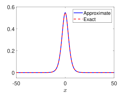
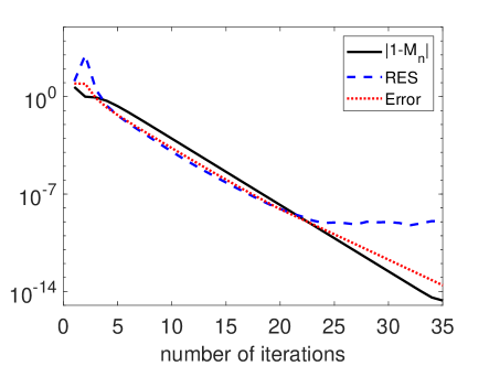
Figure 2.1. Comparison of the exact solution (1.12) with the numerical solution of (1.5) for $\omega=\omega_{0}=4/25$, $\alpha=2$ (left), and the variation of Error$(n)$, $|1-M_{n}|$ and $RES(n)$ with the number of iterations in semi-log scale (right).

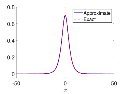
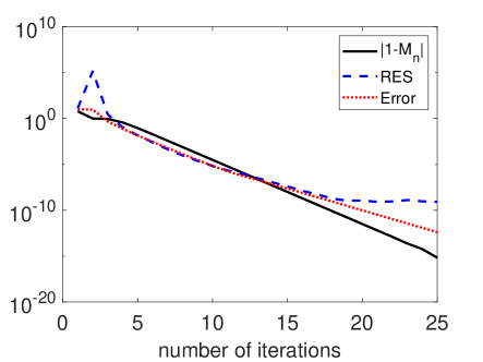
Figure 2.2. Comparison of the exact solution (1.12) with the numerical solution of (1.5) for $\omega=\omega_{0}=9/100$, $\alpha=4$ (left), and the variation of Error$(n)$, $|1-M_{n}|$ and $RES(n)$ with the number of iterations in semi-log scale (right).

The expression in (1.12) gives the exact solution of (1.5) for each $\alpha$ and a fixed $\omega_{0}$. In order to test the accuracy of our scheme, we compare the exact solution (1.12) with the numerical solution. We choose the space interval as $[-200,200]$ and the number of grid points as $N=2^{13}$. In the left panels of Figure 2.1 and Figure 2.2, we show the comparison of the exact solution (1.12) with the numerical solution of (1.5) for $\omega=\omega_{0}=4/25$, $\alpha=2$ and for $\omega=\omega_{0}=9/100$, $\alpha=4$, respectively. The right panels of the figures present the variation of Error$(n)$, $|1-M_{n}|$ and $RES(n)$ with the number of iterations in semi-log scale for the same values of $\alpha$ and $\omega$. We also observe that the $L_{\infty}$ error between the exact and numerical solution is of order $10^{-14}$. These results show that our numerical scheme captures the solution quite well.

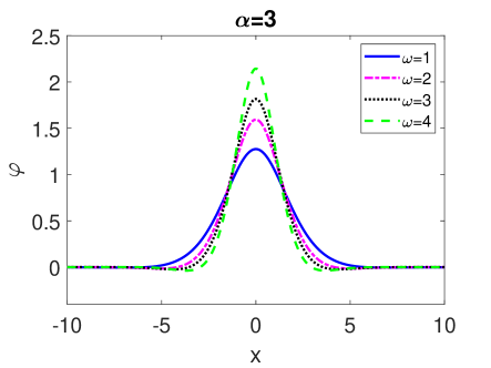
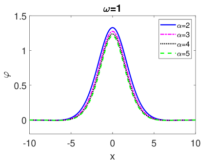
Figure 2.3. Numerical wave profiles for various values of $\omega$, with $\alpha=3$ (left) and numerical wave profiles for various values of $\alpha$ with wave frequency $\omega=1$ (right).

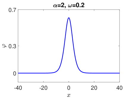
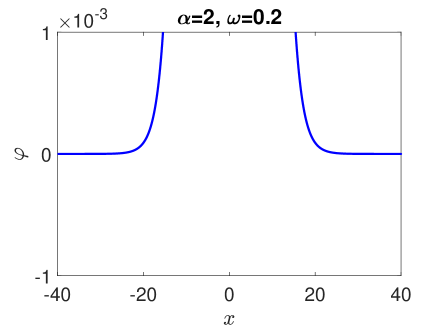
Figure 2.4. The wave profile for $\alpha=2$, $\omega=0.2$ and a close-up look at the profile.

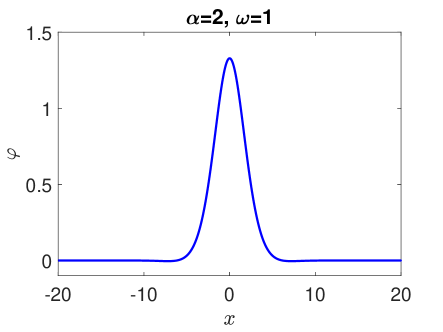
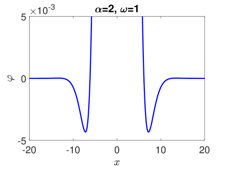
Figure 2.5. The wave profile for $\alpha=2$, $\omega=1$ and a close-up look at the profile.

Now, we generate solutions numerically for several values of $\alpha$ and $\omega\neq\omega_{0}$ where the exact solution does not exist. The left panel of Figure 2.3 shows the profiles of the solutions for a fixed value of $\alpha$ and various values of $\omega$. In the right panel, we present the profiles for a fixed value of $\omega$ and several values of $\alpha$. We observe that the solutions are non-positive for some values of $\alpha$ and $\omega$. For example, the wave profile for $\alpha=2$, $\omega=0.2$ is illustrated in Figure 2.4, and the right panel of the figure gives a closer look at the profile. As it is seen from the figure, the solution is positive. Figure 2.5 shows the wave profile and a closer look for $\alpha=2$, $\omega=1$. In contrast to the previous case, the solution is non-positive. We check the positivity of the solution numerically, by making sure that its minimum value is bigger than $-10^{-15}$. Performing lots of numerical experiments for several values of $\alpha$ and $\omega$, we conclude that the solutions are positive when $\omega<0.25$ and the solutions are non-positive when $\omega>0.25$ for each $\alpha$. Here we also note that, linearizing the equation (1.5) we obtain

$$\varphi^{\prime\prime\prime\prime}-\varphi^{\prime\prime}+\omega\varphi=0.$$ (2.18)

The characteristic equation of (2.18) for a solution of the form $\varphi=e^{\lambda x}$ is

$$\lambda^{4}-\lambda^{2}+\omega=0,$$ (2.19)

where the discriminant is $\Delta=1-4\omega$. This yields that the roots are complex when $\omega<0.25$. In this case, non-positive solutions emanate.

Remark 2.7.

Some important considerations deserve to be explained regarding the numerical solutions obtained in this subsection. The first noteworthy point is that equation $(\ref{edo})$ yields non-positive solutions for specific values of $\alpha$ and $\omega>0.25$. This question is very delicate comparing with similar results in the current literature, as it is well know for the solutions of the standard NLS equation $-\varphi^{\prime\prime}+\omega\varphi-|\varphi|^{\alpha}\varphi=0$ where all smooth solutions that decay at infinity are positive.

Remark 2.8.

As reported in [7, Theorem 1.4], solitary waves that change their sign may occur if $\omega>0.25$. Besides, the solitary waves solve the minimization problem $(\ref{min-problem})$; they also arise as solutions of the problem.

$$\nu_{\omega}:=\inf_{u\in\mathbb{H}^{2}}G_{\omega}(u),$$

where $G_{\omega}(u)=E(u)+\omega F(u)$. Our experiments somehow match with the scenario in [7, Theorem 1.4] since the numerical solutions of $(\ref{edo})$ are non-positive when $\omega>0.25$ for each $\alpha>0$.

3. Spectral analysis

3.1. Brief review of total positivity theory

Our intention is to study the spectrum of the linear operator $\mathcal{L}$ in $(\ref{operator})$ and to do so, we need to consider some tools of the total positivity theory established in [2], [3], and [14]. Let $\mathcal{S}$ be the operator defined on a dense subspace of $L^{2}$ by

$$\mathcal{S}g(x)=Mg(x)+\omega g(x)-(\alpha+1)\psi^{\alpha}(x)g(x),$$ (3.1)

where $\alpha\geq 1$ is real number, $\omega>0$ is a real parameter, $\psi$ is an even real-valued positive solution of the general equation

$$(M+\omega)\psi=\psi^{\alpha+1}.$$ (3.2)

We also assume that function $\psi$ has a suitable decay at infinity and $M$ is defined as a Fourier multiplier operator by

$$\widehat{Mg}(\xi)=m(\xi)\widehat{g}(\xi).$$

Here, the circumflexes notation in the last equality denotes the Fourier transform, $m(\xi)$ is a measurable, locally bounded, even function defined on ${\mathbb{R}}$, and satisfying the following assumptions:
(i) $A_{1}|\xi|^{\mu}\leq m(\xi)\leq A_{2}|\xi|^{\mu}$ for $|\xi|\geq\xi_{0}$,
(ii) $m(\xi)\geq 0$,
where $A_{1}$, $A_{2}$, and $\xi_{0}$ are positive real constants, and $\mu\geq 1$. Under the above assumptions we have the following basic result.

Lemma 3.1.

The operator $\mathcal{S}$ is a closed, unbounded, self-adjoint operator on $L^{2}$ whose spectrum consists of the interval $[\omega,\infty)$ together with a finite number of discrete eigenvalues in the interval $(-\infty,\omega]$, in which all of them have finite multiplicity. In addition, zero is an eigenvalue of $\mathcal{S}$ with eigenfunction $\psi^{\prime}$.

Proof.

See Proposition 1 in [4]. ∎

Next, our intention is to obtain suitable spectral properties for the linear operator $\mathcal{S}$ in $(\ref{opT})$. To this end, let us introduce the family of operators $\mathcal{P}_{\kappa}$, $\kappa\geq 0$, defined on $L^{2}$ as:

$$\mathcal{P}_{\kappa}g(\xi)=\frac{1}{w_{\kappa}(\xi)}\int_{{\mathbb{R}}}K(\xi-y)g(y)dy,$$

where $K(\xi)=(\alpha+1)\widehat{\psi^{\alpha}}(\xi)$ and $w_{\kappa}(\xi)=m(\xi)+\kappa+\omega$. The family of operators $\mathcal{P}_{\kappa}$ act over the Hilbert space

$$X=\left\{g\in L^{2};\,\|g\|_{X,\kappa}=\left(\int_{{\mathbb{R}}}|g(\xi)|^{2}w_{\kappa}(\xi)d\xi\right)^{1/2}<\infty\right\}.$$

By [2, Proposition 2.2], we see that $\mathcal{P}_{\kappa}$ is a compact, self-adjoint operator on $X$ with respect to the norm $\|\cdot\|_{X,\kappa}$. Using the spectral theorem for compact and self-adjoint operators, we conclude that $\mathcal{P}_{\kappa}$ has a family of eigenfunctions $\{\chi_{i,\kappa}\}_{i=0}^{\infty}$ forming an orthonormal basis of $X$. Moreover, the corresponding eigenvalues $\{\lambda_{i}(\kappa)\}_{i=0}^{\infty}$ are real and can be numbered in order of decreasing absolute value:

$$|\lambda_{0}(\kappa)|\geq|\lambda_{1}(\kappa)|\geq\ldots\geq 0.$$

Let us recall some results of [2] and [3]. The first one is concerned with an equivalent formulation of the eigenvalue problem associated with $\mathcal{S}$.

Lemma 3.2.

Suppose $\kappa\geq 0$. Then $-\kappa$ is an eigenvalue of $\mathcal{S}$ (as an operator on $L^{2}$) with eigenfunction $g$ if, and only if, $1$ is an eigenvalue of $\mathcal{P}_{\kappa}$ (as an operator on $X$) with eigenfunction $\widehat{g}$. In particular, both eigenvalues have the same multiplicity.

Proof.

See Corollary 2.3 in [2]. ∎

Since $\mathcal{P}_{\kappa}$ is a compact operator, we have a Krein-Rutman theorem given by the next result.

Lemma 3.3.

The eigenvalue $\lambda_{0}(0)$ of $\mathcal{P}_{0}$ is positive, simple, and has a strictly positive eigenfunction $\chi_{0,0}$. Moreover, $\lambda_{0}(0)>|\lambda_{1}(0)|$.

Proof.

See Lemma 8 in [3]. ∎

Definition 3.4.

A function $f:{\mathbb{R}}\to{\mathbb{R}}$ belongs to the class PF(2) if:
(i) $f(x)>0$ for all $x\in{\mathbb{R}}$,
(ii) for any $x_{1},x_{2},y_{1},y_{2}\in{\mathbb{R}}$ with $x_{1}<x_{2}$ and $y_{1}<y_{2}$, it follows that

$$f(x_{1}-y_{1})f(x_{2}-y_{2})-f(x_{1}-y_{2})f(x_{2}-y_{1})\geq 0,$$

(iii) strict inequality holds in (ii) whenever the intervals $(x_{1},x_{2})$ and $(y_{1},y_{2})$ intersect.

A sufficient condition for a smooth function to be in class $PF(2)$ is that it is logarithmically concave. More precisely, we have:

Lemma 3.5.

Let $f:\mathbb{R}\to\mathbb{R}$ be a positive and twice differentiable function. If $(\log f(x))^{\prime\prime}<0$ for all $x\neq 0$, we have that $f$ belongs to the class PF(2).

Proof.

See Lemma 4.3 in [2] or Lemma 10 in [3]. ∎

Lemma 3.6.

Let $f_{i}:\mathbb{R}\to\mathbb{R}$ be positive and twice differentiable functions, where $i=1,2,\cdots,n$. If $f_{i}$ is a logarithmically concave function for each $i$, then the finite convolution $f_{1}\ast f_{2}\ast\cdots\ast f_{n}$ is also a logarithmically concave function.

Proof.

See [8, Section 3]. ∎

The main theorem in [2] reads as follows.

Theorem 3.7.

Suppose $\widehat{\psi}>0$ on ${\mathbb{R}}$ and $K=(\alpha+1)\widehat{\psi^{\alpha}}\in PF(2)$. Then $\mathcal{S}$ satisfies the following conditions:
(P1) $\mathcal{S}$ has a simple, negative eigenvalue $\kappa$,
(P2) $\mathcal{S}$ has no negative eigenvalue other than $\kappa$,
(P3) the eigenvalue $0$ of $\mathcal{S}$ is simple.

Proof.

See Theorem 3.2 in [2]. ∎

3.2. Spectral analysis for the operator $\mathcal{L}$

In this subsection, we use the total positivity theory determined in previous subsection to get the spectral properties for the general operator $(\ref{operator})$. In fact, as before, since $\mathcal{L}$ is a diagonal operator, its eigenvalues are given by the eigenvalues of the operators $\mathcal{L}_{1}$ and $\mathcal{L}_{2}$ in $(\ref{operator})$.

3.2.1. The spectrum of $\mathcal{L}_{1}$

The operator $\mathcal{L}_{1}$ at the point $\omega=\omega_{0}$ then reads as

$$\mathcal{L}_{1}=\partial_{x}^{4}-\partial_{x}^{2}+\omega_{0}-(\alpha+1)\varphi^{\alpha},$$ (3.3)

where $\varphi=\phi$ is the solitary wave solution with hyperbolic secant profile given by $(\ref{expsolode})$ which is also a minimizer of the problem $(\ref{min-problem})$.

We now can prove the following result.

Proposition 3.8.

The operator ${\mathcal{L}_{1}}$ in (3.3) defined on $L^{2}$ with domain $H^{4}$ has a unique negative eigenvalue, which is simple with positive associated eigenfunction. The eigenvalue zero is simple with associated eigenfunction $\varphi^{\prime}$. Moreover the rest of the spectrum is bounded away from zero and the essential spectrum is the interval $[\omega_{0},\infty)$.

Proof.

By (1.5) we see that $\varphi^{\prime}$ is an eigenfunction of $\mathcal{L}_{1}$ associated with the eigenvalue zero. Also, by Lemma 3.1, the essential spectrum is exactly $[\omega_{0},\infty)$, and since $\varphi$ is a minimizer of the problem $(\ref{min-problem})$, one has that $n(\mathcal{L}_{1})=1$. The only properties that remain to prove in our case is the simplicity of the negative eigenvalue and (P3). We need to observe that $\mathcal{L}_{1}$ is an operator of the form (3.1) with $m(\xi)=\xi^{4}+\xi^{2}$ and $\psi=\varphi$. Thus, it is easy to see that

$$|\xi|^{4}\leq m(\xi)\leq 2|\xi|^{4},\qquad|\xi|\geq 1.$$

Hence, the operator ${\mathcal{L}_{1}}$ satisfies the assumptions in Subsection 3.1 with $A_{1}=1$, $A_{2}=2$, $\mu=4$, and $\xi_{0}=1$. In view of Lemma 3.1 and Theorem 3.7 it suffices to prove that $\widehat{\varphi}>0$ and $\widehat{\varphi^{\alpha}}\in PF(2)$. In fact, by [23, Page 33, Formula 7.5], we first obtain

$$\begin{array}[]{lllll}\widehat{\varphi}(\xi)&=&\displaystyle a_{0}({\rm\,sech}^{\frac{4}{\alpha}}(b_{0}\cdot))^{\wedge}(\xi)=2^{\frac{4}{\alpha}-2}\frac{a_{0}}{b_{0}}\Gamma\left(\frac{4}{\alpha}\right)^{-1}\Gamma\left(\frac{2}{\alpha}+i\frac{\xi}{2b_{0}}\right)\Gamma\left(\frac{2}{\alpha}-i\frac{\xi}{2b_{0}}\right)\\ \\ &=&\displaystyle 2^{\frac{4}{\alpha}-2}\frac{a_{0}}{b_{0}}\Gamma\left(\frac{4}{\alpha}\right)^{-1}\left|\Gamma\left(\frac{2}{\alpha}+i\frac{\xi}{2b_{0}}\right)\right|^{2},\end{array}$$ (3.4)

where $\Gamma$ denotes the usual Gamma function defined by $\Gamma(z)=\int_{0}^{\infty}t^{z-1}e^{-t}dt$ for ${\rm Re}(z)>0$. In addition, in the last equality in $(\ref{fouriersol})$ we have used the property $\Gamma(z)\Gamma(\bar{z})=\Gamma(z)\overline{\Gamma(z)}=|\Gamma(z)|^{2}$. Formula $(\ref{fouriersol})$ gives us automatically that $\widehat{\varphi}>0$ for all $\alpha>0$.
On the other hand, since $\varphi^{\alpha}(x)=a_{0}^{\alpha}{\rm\,sech}^{4}(b_{0}x)$, we obtain by using a similar argument as determined in $(\ref{fouriersol})$

$$\begin{array}[]{llll}\displaystyle\widehat{\varphi^{\alpha}}(\xi)&=&\displaystyle a_{0}^{\alpha}({\rm\,sech}^{4}(b_{0}\cdot))^{\wedge}(\xi)=6\frac{a_{0}^{\alpha}}{b_{0}}\Gamma(4)^{-1}\Gamma\left(2+i\frac{\xi}{2b_{0}}\right)\Gamma\left(2-i\frac{\xi}{2b_{0}}\right)\\ \\ &=&\displaystyle\frac{2a_{0}^{\alpha}}{3b_{0}}\Gamma\left(2\left(1+i\frac{\sqrt{\alpha^{2}+4\alpha+8}}{2\alpha}\xi\right)\right)\Gamma\left(2\left(1-i\frac{\sqrt{\alpha^{2}+4\alpha+8}}{2\alpha}\xi\right)\right).\end{array}$$ (3.5)

We can obtain a convenient expression for $(\ref{fouriesol1})$. To do so, we need to use some properties concerning Gamma function such as $\Gamma(z+1)=z\Gamma(z)$, as well as, non-standard expressions for $\Gamma(2z)$, $\Gamma(1+iy)\Gamma(1-iy)$, and $\Gamma\left(\frac{1}{2}+iy\right)\Gamma\left(\frac{1}{2}-iy\right)$ as found in [1, Page 236, Formulas 6.1.18, 6.1.30 and 6.1.31]. Thus, from $(\ref{fouriesol1})$, we obtain the final and simplified expression

$$\widehat{\varphi^{\alpha}}(\xi)=\frac{a_{0}^{\alpha}}{3b_{0}^{2}}\left(\frac{1}{4}+\frac{\alpha^{2}+4\alpha+8}{4\alpha^{2}}\xi^{2}\right)\frac{\pi}{\cosh\left(\frac{\pi}{4b_{0}}\xi\right)}\frac{\xi}{\sinh\left(\frac{\pi}{4b_{0}}\xi\right)}.$$ (3.6)

The expression $(\ref{fouriesol2})$ gives us that $\widehat{\varphi^{\alpha}}>0$. In addition, let us consider the function $\beta(x)={\rm\,sech}(b_{0}x)$. Using the arguments in [23, Page 33, Formula 7.1], we deduce $\widehat{\beta}(\xi)=\frac{\pi}{2b_{0}}{\rm\,sech}\left(\frac{\pi\xi}{2b_{0}}\right)$ and $\widehat{\beta}>0$ belongs to the class $PF(2)$, since

$$\frac{d^{2}}{d\xi^{2}}\log(\widehat{\beta}(\xi))=-\frac{\pi^{2}}{4b_{0}^{2}}{\rm\,sech}^{2}\left(\frac{\pi\xi}{2b_{0}}\right)<0.$$

Thus, from Lemma 3.6, we have that $\widehat{\varphi^{\alpha}}$ belongs to the class $PF(2)$, that is, $K=(\alpha+1)\widehat{\varphi^{\alpha}}\in PF(2)$ as desired. ∎

3.2.2. The spectrum of $\mathcal{L}_{2}$

By Proposition 2.6, we have determined that the number of negative eigenvalues of $\mathcal{L}_{2}$ is zero since $n(\mathcal{L})=n(\mathcal{L}_{1})+n(\mathcal{L}_{2})=1$ and $n(\mathcal{L}_{1})=1$. However, we need to calculate $z(\mathcal{L}_{2})$ in order to conclude that $z(\mathcal{L})=2$. To do so, we have the following result:

Proposition 3.9.

The operator $\mathcal{L}_{2}=\partial_{x}^{4}-\partial_{x}^{2}+\omega-\varphi^{\alpha}$ defined on $L^{2}$ with domain $H^{4}$ has no negative eigenvalues. The eigenvalue zero is simple with associated eigenfunction $\varphi$. Moreover the rest of the spectrum is bounded away from zero and the essential spectrum is the interval $[\omega_{0},\infty)$.

Proof.

First, by Proposition 2.6, we automatically obtain that $n(\mathcal{L}_{2})=0$. We need to prove that $0$ is a simple eigenvalue of $\mathcal{L}_{2}.$ This result, in fact, is not explicitly covered by the arguments in Subsection 3.1, but we can still adapt it to the linear operator $\mathcal{L}_{2}$. Indeed, the essential spectrum is $[\omega_{0},\infty)$ and this fact is due to Lemma 3.1. In view of $(\ref{edo})$, it is clear that zero is an eigenvalue with eigenfunction $\varphi$. Thus, Lemma 3.2 implies that $1$ is an eigenvalue of $\mathcal{P}_{0}$ with eigenfunction $\widehat{\varphi}$. We claim that: if $\lambda_{0}(0)$ is the first eigenvalue of $\mathcal{P}_{0}$, we have $\lambda_{0}(0)=1$. In fact, let us assume by contradiction that $\lambda_{0}(0)$ is the first eigenvalue of $\mathcal{P}_{0}$ and $\lambda_{0}(0)\neq 1$. Consider $\chi_{0,0}$ be the eigenfunction associated to $\lambda_{0}(0)$. Using Lemma 3.3, we have $\chi_{0,0}>0$. Since $\mathcal{L}_{2}\varphi=0$ and $\widehat{\varphi}>0$, by Proposition 3.8, the inner product in $L^{2}$ between $\chi_{0,0}$ and $\widehat{\varphi}$ is then strictly positive, which contradicts the fact that the eigenfunctions are orthogonal.
Gathering the above claim and Lemma 3.3, we obtain that 1 is a simple eigenvalue of $\mathcal{S}_{0}$. Therefore, it follows from Lemma 3.2 that zero is a simple eigenvalue of $\mathcal{L}_{2}$.

∎

3.3. The spectrum of $\mathcal{L}$

We state the spectral properties of the linearized operator $\mathcal{L}$ at $\omega=\omega_{0}$ and for $\varphi=\phi$ given by $(\ref{expsolode}).$ To prove next proposition, we use the results contained in Propostions 3.8 and 3.9.

Proposition 3.10.

The operator $\mathcal{L}$ in (1.10) defined on $\mathbb{L}^{2}$ with domain $\mathbb{H}^{4}$ has a unique negative eigenvalue, which is simple. The eigenvalue zero is double with associated eigenfunctions $(\varphi^{\prime},0)$ and $(0,\varphi)$. Moreover the essential spectrum is the interval $[\omega_{0},\infty)$.

$\blacksquare$

4. Orbital stability and instability of solitary waves

4.1. Local and global well-posedness

Let us recall some important results concerning the local and global well-posedness for the Cauchy problem associated to the equation $(\ref{NLS-equation})$ given by

$$\left\{\begin{array}[]{llll}iu_{t}+u_{xx}-u_{xxxx}+|u|^{\alpha}u=0,\ \ \ \ \ \ \mbox{in}\ \mathbb{R}\times\mathbb{R},\\ \\ u(x,0)=u_{0}(x),\ \ \ \ \ \ \ \ \ \ \ \ \ \ \ \ \ \ \ \ \ \ \ \ \ \mbox{in}\ \mathbb{R}.\end{array}\right.$$ (4.1)

Proposition 4.1.

Given $u_{0}\in\mathbb{H}^{2}$, there exists $t_{0}>0$ and a unique solution $u\in C([0,t_{0}];\mathbb{H}^{2})$ of (4.1) such that $u(0)=u_{0}$. The solution conserves the energy and the mass in the sense that

$$E(u(t))=E(u_{0})\quad\mbox{and}\quad F(u(t))=F(u_{0})\quad t\in[0,t_{0}],$$

where $E$ is defined in (1.3) and $F$ is defined in (1.4). Let $t^{*}$ be the maximal time of existence of $u$. Then either

• $t^{*}=\infty$, or

• $t^{*}<\infty$ and $\lim_{t\to t^{*}}\|u(t)\|_{\mathbb{H}^{2}}=\infty$.

Moreover, for any $s<t^{*}$ the data-solution mapping $u_{0}\mapsto u$ is continuous from $\mathbb{H}^{2}$ to $C([0,s];\mathbb{H}^{2})$.

Proof.

See Proposition 4.1 in [27]. ∎

Regarding global solutions in the energy space $\mathbb{H}^{2}$, we have the following result.

Corollary 4.2.

Let $u_{0}\in\mathbb{H}^{2}$ be fixed. If $0<\alpha<8$, then the solution $u$ obtained in Theorem Proposition 4.1 can be extended to the whole real line.

Proof.

We need to use the conservation law $E(u(t))=E(u_{0})$ for all $t\in[0,t^{\ast})$, and the Gagliardo-Nirenberg inequality in [18, Chapter 3]. In fact, the term $||u(t)||_{\mathbb{L}^{\alpha+2}}^{\alpha+2}$ present in $(\ref{E})$ can be estimated by

$$||u(t)||_{\mathbb{L}^{\alpha+2}}\leq C||u_{xx}(t)||_{\mathbb{L}^{2}}^{\theta}||u(t)||_{\mathbb{L}^{2}}^{1-\theta},$$ (4.2)

where $\theta=\frac{\alpha}{4(\alpha+2)}$ and $C>0$ is a constant. By using $E(u(t))=E(u_{0})$ and $F(u(t))=F(u_{0})$, we obtain from inequality in $(\ref{GN1})$ that

$$\begin{array}[]{llll}||u_{xx}(t)||_{\mathbb{L}^{2}}^{2}&\leq&\displaystyle E(u(t))+\int_{\mathbb{R}}|u(x,t)|^{\alpha+2}dx=E(u_{0})+\int_{\mathbb{R}}|u(x,t)|^{\alpha+2}dx\\ \\ &\leq&E(u_{0})+C||u_{xx}(t)||_{\mathbb{L}^{2}}^{\frac{\alpha}{4}}||u_{0}||_{\mathbb{L}^{2}}^{\frac{3\alpha+8}{4}}.\end{array}$$ (4.3)

On the other hand, since $\left(||u_{xx}||_{\mathbb{L}^{2}}^{2}+||u||_{\mathbb{L}^{2}}^{2}\right)^{\frac{1}{2}}$ is an equivalent norm in $\mathbb{H}^{2}$, we obtain by $(\ref{GN2})$ that the local solution $u$ obtained in Proposition 4.1 is global in the energy space $\mathbb{H}^{2}$ when $\alpha\in(0,8)$. ∎

4.2. Orbital stability and instability

We first make clear our notion of orbital stability. Taking into account that (1.1) is invariant by rotations and translations, we define the orbit generated by $\Phi=(\varphi,0)$ as

$$\begin{split}\Omega_{\Phi}&=\{T_{1}(\theta)T_{2}(r)\Phi;\;\;\theta,r\in{\mathbb{R}}\}\\ &=\left\{\left(\begin{array}[]{cc}\cos\theta&\sin\theta\\ -\sin\theta&\cos\theta\end{array}\right)\left(\begin{array}[]{c}\varphi(\cdot-r)\\ 0\end{array}\right);\;\;\theta,r\in{\mathbb{R}}\right\}.\end{split}$$ (4.4)

In $\mathbb{H}^{2}$, we introduce the pseudo-metric $d$ by $d(f,g):=\inf\{\|f-T_{1}(\theta)T_{2}(r)\Phi\|_{\mathbb{H}^{2}};\;\theta,r\in{\mathbb{R}}\}.$

We have to notice that the distance between $f$ and $g$ is the distance between $f$ and the orbit generated by $g$ under the actions of rotation and translation, that is, $d(f,\Phi)=d(f,\Omega_{\Phi}).$ We have the following definition of orbital stability:

Definition 4.3.

Let $\Theta(x,t)=e^{i\omega t}\varphi(x)=(\varphi(x)\cos(\omega t),\varphi(x)\sin(\omega t))$ be a standing wave for (1.1). We say that $\Theta$ is orbitally stable in $\mathbb{H}^{2}$ provided that, given ${\varepsilon}>0$, there exists $\delta>0$ with the following property: if $u_{0}\in\mathbb{H}^{2}$ satisfies $\|u-\Phi\|_{\mathbb{H}^{2}}<\delta$, then the solution, $u(t)$, of (1.1) with initial condition $u_{0}$ exist for all $t\geq 0$ and satisfies $d(u(t),\Omega_{\Phi})<{\varepsilon},\ \mbox{for all}\ t\geq 0.$ Otherwise, we say that $\Theta$ is orbitally unstable in $\mathbb{H}^{2}$.

We have the following stability result.

Proposition 4.4.

Let $\varphi$ be an even minimizer of the problem 2.2. If $z(\mathcal{L})=2$, $d^{\prime\prime}(\omega)>0$ and the Cauchy problem in $(\ref{CauchyNLS})$ is globally well-posed in the energy space $\mathbb{H}^{2}$, then the minimizer $\varphi$ is orbitally stable in the sense of Definition 4.3.

Proof.

Since $\varphi$ is an even minimizer of the problem $(\ref{min-problem})$, we obtain by the proof of Propositon 2.6 that $n(\mathcal{L})=1$. This fact imply, $n(\mathcal{L})=1$ and $z(\mathcal{L})=2$ with ${\rm\,Ker}(\mathcal{L})=[(\varphi^{\prime},0),(0,\varphi)]$. Since $d^{\prime\prime}(\omega)>0$ and the Cauchy problem in $(\ref{CauchyNLS})$ is globally well-posed in the energy space $\mathbb{H}^{2}$, we obtain by the arguments in [29] (see also [22]) that $\varphi$ is orbitally stable in the sense of Definition 4.3. ∎

Let $\mathbb{H}_{e}^{2}$ be the space constituted by complex functions $v\in\mathbb{H}^{2}$ such that $v$ is even. In $\mathbb{H}_{e}^{2}$, we can consider the Cauchy problem in $(\ref{CauchyNLS})$ to study the local and global well-posedness of even solutions in the sense that the results of Proposition 4.1 and Corollary 4.2 can be easily adapted for this particular case. The only feature that we lost in our analysis is that over $\mathbb{H}_{e}^{2}$, the equation in $(\ref{CauchyNLS})$ is not invariant under the symmetry of translations, and this means that it is necessary to remove the action $T_{2}$ in the Definition of stability 4.3. Since the associated operator $\mathcal{L}_{e}=\left(\begin{array}[]{cccc}\mathcal{L}_{1,e}&0\\ 0&\mathcal{L}_{2,e}\end{array}\right):D(\mathcal{L}_{e})=\mathbb{H}_{e}^{2}\subset\mathbb{L}_{e}^{2}\rightarrow\mathbb{L}_{e}^{2}$ has the same form as $\mathcal{L}$ in $(\ref{operator})$ and is invariant over the space $\mathbb{L}_{e}^{2}$ constituted by functions in $\mathbb{L}^{2}$ that are even, we obtain immediately when $\varphi$ is an even minimizer of the problem $(\ref{min-problem})$ that $n(\mathcal{L}_{e})=1$ (this would happen when $\alpha$ is an even integer according to Remark 2.5). On the other hand, if $\varphi$ is even, we obtain that $\varphi^{\prime}$ is odd and this implies $(\varphi^{\prime},0)$ is not an element of ${\rm\,Ker}(\mathcal{L}_{e})$. Both facts enable us to use [10] to conclude the following result:

Proposition 4.5.

Let $\varphi$ be an even minimizer of the problem 2.2 and suppose $z(\mathcal{L}_{e})=1$.
i) If $d^{\prime\prime}(\omega)>0$, then the minimizer $\varphi$ is orbitally stable in $\mathbb{H}_{e}^{2}$ in the sense of Definition 4.3 only modulus rotations.
ii) If $d^{\prime\prime}(\omega)<0$, then the minimizer $\varphi$ is orbitally unstable in $\mathbb{H}_{e}^{2}$ in the sense of Definition 4.3 only modulus rotations. Therefore, $\phi$ is orbitally unstable in $\mathbb{H}^{2}$ in the sense of Definition 4.3.

Proof.

Item i) follows by [10, Theorem 3.5], while item ii) is a consequence of [10, Theorem 4.7].

∎

4.3. Numerical study of $d^{\prime\prime}(\omega)$

Now, we will study the sign of $\displaystyle d^{\prime\prime}(\omega)=\frac{1}{2}\frac{d}{d\omega}\int_{\mathbb{R}}\varphi^{2}(x)dx,$ numerically. To give an analytical support for this study in a neighbourhood of $\omega_{0}$, we first need to prove the following result:

Proposition 4.6.

Let $\varphi$ be the solution of $(\ref{edo})$ given by $(\ref{expsolode})$. For each $\alpha>0$, there exists a neighborhood $I_{\alpha}$ centered at $\omega_{0}$, an open ball $B$ in $H^{4}$ centered at $\varphi$, and a unique smooth curve $\omega\in I_{\alpha}\mapsto\varphi_{\omega}\in B\subset H^{4}$ of even positive solutions for the equation $(\ref{edo})$.

Proof.

Let us define the map $\Upsilon:(0,+\infty)\times H_{e}^{4}\rightarrow L_{e}^{2}$ given by

$$\Upsilon(\omega,\psi)=\psi^{\prime\prime\prime\prime}-\psi^{\prime\prime}+\omega\psi-\psi^{\alpha+1},$$ (4.5)

where $L_{e}^{4}$ and $H_{e}^{4}$ are the spaces $L^{2}$ and $H^{4}$, respectively, constituted by even functions. We see from equation $(\ref{edo})$ that $\Upsilon(\omega_{0},\varphi)=0$. Additionally, the function $\Upsilon$ is smooth in all variables, and the Fréchet derivative at the point $(\omega_{0},\varphi)$ is

$$D_{\psi}\Upsilon(\omega_{0},\varphi)=\partial_{x}^{4}-\partial_{x}^{2}+\omega_{0}-(\alpha+1)\varphi^{\alpha}=\mathcal{L}_{1,e}.$$ (4.6)

Since $\varphi$ is even, $\varphi^{\prime}$ is odd and it is not an element in $H_{e}^{4}$. By Proposition 3.8, we obtain that $0$ is an isolated simple eigenvalue associated with the eigenfunction $\varphi^{\prime}$, the remainder of the spectrum is bounded away from zero, and the essential spectrum is the interval $[\omega_{0},+\infty)$. Thus, we conclude that $0$ is not an element of the spectrum of the operator $\mathcal{L}_{1,e}$ over the space $L_{e}^{2}$, which implies that $0$ belongs to the resolvent set of $\mathcal{L}_{1,e}$. From the implicit function theorem, we obtain a neighborhood $I_{\alpha}$ centered at $\omega_{0}$, an open ball $B$ in $H^{4}$ centered at $\varphi$, and a unique smooth curve $\omega\in I_{\alpha}\mapsto\varphi_{\omega}\in B\subset H^{4}$ of solutions for the equation $(\ref{edo})$. This fact proves the proposition. ∎

To explore the sign of $d^{\prime\prime}(\omega)$, the integral is approximated by the trapezoidal rule and the derivative is calculated by a forward difference approximation. Figure 4.1 shows the values of $\displaystyle d^{\prime\prime}(\omega)$ for $\alpha=2,~{}3,~{}4,~{}5$. The dashed vertical lines in the rest of the figures correspond to the $\omega_{0}$ value where the exact solution exists. The graphs show that $d^{\prime\prime}(\omega)>0$ when $\alpha\leq 4$; however, the sign changes from negative to positive at a threshold $\omega$ value for $\alpha=5.$ Therefore, we next focus on the interval $\alpha\in(4,5)$. Figure 4.2 illustrates the variation of $d^{\prime\prime}(\omega)$ with $\omega$ for $\alpha=4.2$ and $\alpha=4.3$. These experiments show that the sign-changing behavior begins with $\alpha\approx 4.3$. It can be seen from Figure 4.3 the sign of $d^{\prime\prime}(\omega)$ changes at $\omega=\omega_{0}$ for $\alpha\approx 4.8$. Finally, we consider the values where $\alpha>5$. We present the variation of $d^{\prime\prime}(\omega)$ with $\omega$ for $\alpha=5.4$ and $\alpha=5.5$ in Figure 4.4. The result shows that $d^{\prime\prime}(\omega)$ becomes negative for all $\omega$ values when $\alpha\geq 5.5$. Our results indicate a prediction for the orbital stability since for $\alpha\in(0,4.3)$, we have $d^{\prime\prime}(\omega)>0$. If $\alpha\in[4.3,5.5)$, we obtain a threshold value $\omega_{c}$ such that if $\omega\in(0,\omega_{c})$, we have $d^{\prime\prime}(\omega)<0$, and if $\omega>\omega_{c}$, we obtain $d^{\prime\prime}(\omega)>0$. At $\omega=\omega_{c}$, we deduce that $d^{\prime\prime}(\omega_{c})=0$, that is, we obtain a frequency $\omega$ that indicates a critical value for the stability. When $\alpha\geq 5.5$, we obtain that $d^{\prime\prime}(\omega)<0$.

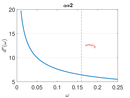
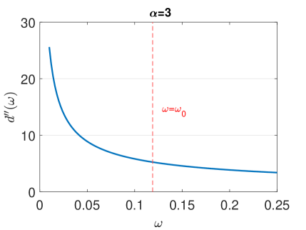
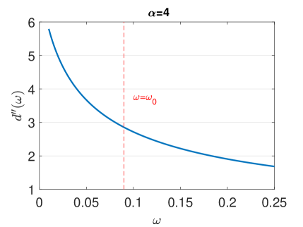
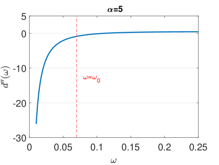
Figure 4.1. The variation of $d^{\prime\prime}(\omega)$ with $\omega$ for $\alpha=2,~{}3,~{}4,~{}5$.

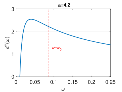
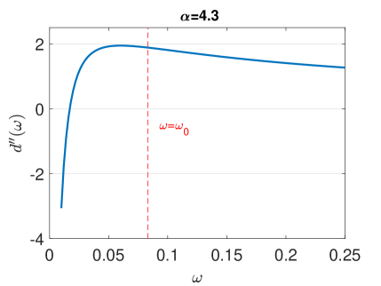
Figure 4.2. The variation of $d^{\prime\prime}(\omega)$ with $\omega$ for $\alpha=4.2$ and $\alpha=4.3$.

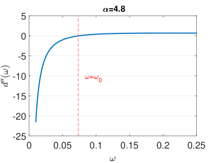
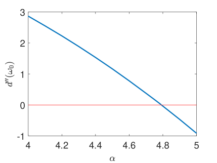
Figure 4.3. The variation of $d^{\prime\prime}(\omega)$ with $\omega$ for $\alpha=4.8$ and the variation of $d^{\prime\prime}(\omega_{0})$ with $\alpha$.

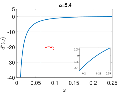
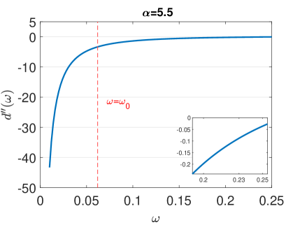
Figure 4.4. The variation of $d^{\prime\prime}(\omega)$ with $\omega$ for $\alpha=5.4$ and $\alpha=5.5$.

Proof of Theorem 1.1. By Proposition 3.10, we obtain that $n(\mathcal{L})=1$ and $z(\mathcal{L})=2$. In addition, since $\phi^{\prime}=\varphi^{\prime}$ is odd, we obtain $n(\mathcal{L}_{e})=1$ and $z(\mathcal{L}_{e})=1$. According to Figures 4.1-4.4, we see that $d^{\prime\prime}(\omega_{0})>0$ for all $\alpha\in(0,\alpha_{0})$, while $d^{\prime\prime}(\omega_{0})<0$ for all $\alpha>\alpha_{0}$. Important to mention that it is possible to see in Figure 4.3 the threshold value where $d^{\prime\prime}(\omega_{0})=0$. For $\alpha_{0}<\alpha_{0}$, we can use Proposition 4.4 to conclude that $\varphi$ in $(\ref{expsolode})$ is orbitally stable in $\mathbb{H}^{2}$. On the other hand, if $\alpha>\alpha_{0}$ we obtain that $\varphi$ is orbitally unstable in $\mathbb{H}^{2}$ according to the Proposition 4.5-ii).

$\blacksquare$

Remark 4.7.

Some important considerations need to be highlighted. The first one is that the presence of the mixed term $\partial_{x}^{4}-\partial_{x}^{2}$ in equation $(\ref{NLS-equation})$ causes the surprising fact that even though the parameter $\alpha$ belongs to an interval where the existence of global solutions for the Cauchy problem $(\ref{CauchyNLS})$, namely $\alpha\in(\alpha_{0},8)$, we have that the minimizer $\varphi$ in $(\ref{expsolode})$ is orbitally unstable in $\mathbb{H}^{2}$. This fact is a novelty compared with the NLS equation $(\ref{2NLS-equation})$ since parameter $\alpha$ for the existence of a global solution in $\mathbb{H}^{1}$ and the orbital stability are the same, that is, if $\alpha\in(0,4)$ we have global solutions and stability and if $\alpha\in(4,+\infty)$ we obtain blow-up phenomena and instability. As far as we know, we have a similar scenario if we remove the term $u_{xx}$ in $(\ref{NLS-equation})$ to deal with the equation

$$iu_{t}-u_{xxxx}+|u|^{\alpha}u=0.$$ (4.7)

The scaling invariance $u\mapsto\lambda^{\frac{4}{\alpha}}u(\lambda x,\lambda^{4}t)$ associated with the equation $(\ref{4NLS})$ predicts that we would have global solutions and orbital stability for $\alpha\in(0,8)$. Blow-up phenomena and instability may occur when $\alpha>8$. On the other hand, the prediction for the stability/instability can be easily determined since we have the equality

$$d^{\prime\prime}(\omega)=\frac{1}{2\omega}\left(\frac{8-\alpha}{2\alpha}\right)\int_{\mathbb{R}}\varphi^{2}(x)dx.$$ (4.8)

References

- [1] M. Abramowitz and I.A. Stegun, Handbook of Mathematical Functions: With Formulas, Graphs, and Mathematical Tables, Dover, New York, 1970.
- [2] J.P. Albert, Positivity properties and stability of solitary-wave solutions of model equations for long waves, Commun. Partial Differ. Equ., 17 (1992), 1–22.
- [3] J.P. Albert and J.L. Bona, Total positivity and the stability of internal waves in stratified fluids of finite depth, IMA J. Appl. Math., 46 (1991), 1–19.
- [4] J.P. Albert, J.L. Bona, and D. Henry, Sufficient conditions for instability of solitary-wave solutions of model equation for long waves, Physica D, 24 (1987), 343–366.
- [5] H. Berestycki and T. Cazenave, Instabilité des états stationnaires dans les équations de Schrödinger et de Klein–Gordon non linéaires, C. R. Acad. Sci. Paris Sér. I Math., 293 (1981), 489–492.
- [6] D. Bonheure, J.P. Castreras, E.M. dos Santos, and R. Nascimento, Orbitally stable standing waves of a mixed dispersion nonlinear Schrödinger equation, SIAM J. Math. Anal., 50 (2018), 5027-5071.
- [7] D. Bonheure and R. Nascimento, Waveguide Solutions for a Nonlinear Schrödinger Equation with Mixed Dispersion. In Contributions to Nonlinear Elliptic Equations and Systems, 31–53. Progress in Nonlinear Differential Equations and Their Application 86. Cham: Birkhäuser/Springer, 2015.
- [8] H.J. Brascamp and E.H. Lieb, On extensions of the Brunn-Minkowski and Prékopa-Leindler theorems, including inequalities for log concave functions, and with an application to the di®usion equation, J. Funct. Anal. 22 (1976), 366-389.
- [9] A. Duran, An efficient method to compute solitary wave solutions of fractional Korteweg–de Vries equations, Int. J. Comput. Math. 95 (2018), 1362–1374.
- [10] M. Grillakis, J. Shatah, and W. Strauss, Stability theory of solitary waves in the presence of symmetry I, J. Funct. Anal., 74 (1987), 160–197.
- [11] M. Grillakis, J. Shatah, and W. Strauss, Stability theory of solitary waves in the presence of symmetry II, J. Funct. Anal., 74 (1990), 308–348.
- [12] U. Le and D. Pelinovsky, Convergence of Petviashvili’s method near periodic waves in the fractional Korteweg-de Vries equation, SIAM J. Math. Anal., 51 (2019), 2850-2883.
- [13] S. Levandosky, A stability analysis of fifth-order water wave models, Physica D, 125 (1999), 222-240.
- [14] S. Karlin, Total Positivity, Stanford Univ. Press, Stanford, 1968.
- [15] V.I. Karpman, Stabilization of soliton instabilities by higher-order dispersion: fourth order nonlinear Schrödinger-type equations, Phys. Rev. E, 53 (1996), 1336–1339.
- [16] V.I. Karpman and A.G. Shagalov, Stability of soliton described by nonlinear Schrödinger type equations with higher-order dispersion, Physica D, 144 (2000), 194–210.
- [17] E. Lenzmann and J. Sok, A sharp rearrangement principle in Fourier space and symmetry results for PDEs with arbitrary order, Int. Math. Res. Notices, (2021), 15040–15081.
- [18] F. Linares and G. Ponce, Introduction to nonlinear dispersive equations, Springer, NY, 2008.
- [19] P.L. Lions, The concentration compactness principle in the calculus of variations. The locally compact case, part I, Annal. Inst. Henri Poincaré. Analyse non Linéaire, 1 (1984), 109-145.
- [20] P.L. Lions, The concentration compactness principle in the calculus of variations. The locally compact case, part II, Annal. Inst. Henri Poincaré. Analyse non Linéaire, 1 (1984), 223-283.
- [21] G.E.B. Moraes, H. Borluk, G. de Loreno, G.M. Muslu and F. Natali, Orbital stability of periodic standing waves for the cubic fractional nonlinear Schrödinger equation. J. Differ. Equ., (2022) 341, pp.263-291.
- [22] F. Natali and A. Pastor, The fourth-order dispersive nonlinear Schrödinger equation: Orbital stability of a standing wave, SIAM Journal of Appl. Dyn. System, 14 (2015), 1326-1346.
- [23] F. Oberhettinger, Tables of Fourier transforms and Fourier transforms of distributions, Springer-Verlag, Berlin-Heidelberg, 1990.
- [24] G. Oruc, H. Borluk and G.M. Muslu, The generalized fractional Benjamin-Bona-Mahony equation: Analytical and numerical results, Phys. D, 409 (2020), 132499.
- [25] G. Oruc, F. Natali, H. Borluk and G.M. Muslu, On the stability of solitary wave solutions for a generalized fractional Benjamin–Bona–Mahony equation, Nonlinearity, 35 (2022), 1152-1169.
- [26] D. Pelinovsky and Y. Stepanyants, Convergence of Petviashvili’s iteration method for numerical approximation of stationary solution of nonlinear wave equations, SIAM J. Numer. Anal., 42 (2004), 1110-1127
- [27] B. Pausader, Global well-posedness for energy critical fourth-order Schrödinger equations in the radial case, Dynamics of PDE, 4 (2007), 197–225.
- [28] M. Reed and B. Simon, Methods of modern mathematical physics IV. Analysis of operators, Academic Press, New York-London, 1978.
- [29] M.I. Weinstein, Lyapunov stability of ground states of nonlinear dispersive evolutions equations, Comm. Pure Appl. Math. 39 (1986), 51–68.
- [30] M.I. Weinstein, Nonlinear Schrödinger equations and sharp interpolation estimates, Comm. Math. Phys., 87 (1983), 567–576.