Algebraic Tools for Computing Polynomial Loop Invariants

Abstract.

Loop invariants are properties of a program loop that hold before and after each iteration of the loop. They are often employed to verify programs and ensure that algorithms consistently produce correct results during execution. Consequently, the generation of invariants becomes a crucial task for loops. We specifically focus on polynomial loops, where both the loop conditions and assignments within the loop are expressed as polynomials. Although computing polynomial invariants for general loops is undecidable, efficient algorithms have been developed for certain classes of loops. For instance, when all assignments within a while loop involve linear polynomials, the loop becomes solvable. In this work, we study the more general case where the polynomials exhibit arbitrary degrees.

Applying tools from algebraic geometry, we present two algorithms designed to generate all polynomial invariants for a while loop, up to a specified degree. These algorithms differ based on whether the initial values of the loop variables are given or treated as parameters. Furthermore, we introduce various methods to address cases where the algebraic problem exceeds the computational capabilities of our methods. In such instances, we identify alternative approaches to generate specific polynomial invariants.

1. Introduction

Loop invariants denote properties that hold both before and after each iteration of a loop within a given program. They play a crucial role in automating the program verification, ensuring that algorithms consistently yield correct results prior to execution. Notably, various recognized methods for safety verification like the Floyd–Hoare inductive assertion technique (Floyd, 1993) and the termination verification via standard ranking functions technique (Manna and Pnueli, 2012) rely on loop invariants to verify correctness, ensuring complete automation in the verification process.

In this work, we focus on polynomial loops, wherein expressions within assignments and conditions are polynomials equations in program variables. More precisely, a polynomial loop is of the form:

$(x_{1},x_{2},\ldots,x_{n})=(a_{1},a_{2},\ldots,a_{n})$ while $g_{1}=\cdots=g_{k}=0$ do      $\begin{pmatrix}x_{1}\\ x_{2}\\ \vdots\\ x_{n}\end{pmatrix}\xleftarrow{\textbf{F}}\begin{pmatrix}f_{1}\\ f_{2}\\ \vdots\\ f_{n}\end{pmatrix}$ end while

where the $x_{i}$’s represent program variables with initial values $a_{i}$, and $g_{i}$’s and $f_{i}$’s are polynomials in the program variables. Computing polynomial invariants for loops has been a subject of study over the past two decades, see e.g. (de Oliveira et al., 2017; Kovács, 2023; Amrollahi et al., 2022; Hrushovski et al., 2018; Karr, 1976; Kovács, 2008; Rodríguez-Carbonell and Kapur, 2004, 2007a, 2007b). Computing polynomial invariants for general loops is undecidable (Hrushovski et al., 2023). Therefore, particular emphasis has been placed on specific families of loops, especially those in which the assertions are all linear or can be reduced to linear assertions. In the realm of linear invariants, Michael Karr introduced an algorithm pioneering the computation of all linear invariants for loops where each assignment within the loop is a linear function (Karr, 1976). Subsequent studies, such as (Müller-Olm and Seidl, 2004b) and (Rodríguez-Carbonell and Kapur, 2007a), have demonstrated the feasibility of computing all polynomial invariants up to a specified degree for loops featuring linear assignments. Further, the problem of generating all polynomial invariants for loops with linear assignments, are studied in (Hrushovski et al., 2018) and (Rodríguez-Carbonell and Kapur, 2007a).

Another class of loops for which invariants have been successfully computed is the family of solvable loops. These loops are characterized by polynomial assignments that are either inherently linear or can be transformed into linear forms through a change of variables, as elaborated in (de Oliveira et al., 2016) and (Kovács, 2008). Nonetheless, challenges persist when dealing with loops featuring non-linear or unsolvable assignments, as discussed in (Rodríguez-Carbonell and Kapur, 2007b) and (Amrollahi et al., 2022).

Before stating our main results, we introduce some terminology from algebraic geometry. We refer to (Cox et al., 2013; Kempf, 1993) for further details. Let $\mathbb{C}$ denote the field of complex numbers. Let $S$ be a set of polynomials in $\mathbb{C}[x_{1},\ldots,x_{n}]$, then the algebraic variety $\bm{V}(S)$ associated to $S$ is the common zero set of all polynomials in $S$. Here, $\bm{V}(S)=\bm{V}(\langle S\rangle)$, where $\langle S\rangle$ is the ideal generated by $S$. Conversely, the defining ideal of a subset $X\subset\mathbb{C}^{n}$ is the set of polynomials in $\mathbb{C}[x_{1},\ldots,x_{n}]$ that vanish on $X$. The algebraic variety associated to the ideal $I(X)$ is called the Zariski closure of $X$. Therefore, if $X$ is an algebraic variety, then $\bm{V}(I(X))=X$. Moreover, $X_{1}\subseteq X_{2}$ implies that $I(X_{2})\subseteq I(X_{1})$. A map $F:\mathbb{C}^{n}\to\mathbb{C}^{m}$ is called a polynomial map, if there exist $f_{1},\ldots,f_{m}$ in $\mathbb{C}[x_{1},\ldots,x_{n}]$, such that $F(x)=(f_{1}(x),\ldots,f_{m}(x))$ for all $x\in\mathbb{C}^{n}$. For the sake of simplicity, in what follows we will refer to polynomial maps and their associated polynomials interchangeably.

We now define the main object introduced in this paper.

Definition 1.1.

Let $F:\mathbb{C}^{n}\longrightarrow\mathbb{C}^{n}$ be a polynomial map and $X\subseteq\mathbb{C}^{n}$ an algebraic variety. The invariant set of $(F,X)$ is defined as:

$S_{(F,X)}=\{x\in X\mid\forall m\in\mathbb{N},F^{(m)}(x)\in X\},$

where $F^{(0)}(x)=x$ and $F^{(m)}(x)=F(F^{(m-1)}(x))$ for any $m>1$.

Our contributions. In this work, we consider the problem of generating polynomial invariants for loops with polynomial maps of arbitrary degrees. Our contributions are as follows:

1. We design Algorithm 1 to compute invariant sets and use it to decide if a given polynomial is invariant (Proposition 3.5).

2. We design two algorithms for computing polynomial invariants of a loop up to a fixed degree. The first one (Theorem 3.6), when the initial value is not fixed, outputs a linear parametrization which depends polynomially on this value. The second (Algorithm 2), when the initial value is fixed, is much more efficient and computes a basis of this set, seen as a vector space. Experiments with our prototype implementation demonstrate the practical efficiency of our algorithms, solving problems beyond the current state of the art. Note that the algorithms can be adjusted to include disequalities in the guard; see Remarks 3 and 4.

3. Finally, we apply these algorithms to other problems: we show how to lift some polynomial invariants for the non-fixed initial value case from the fixed one (Proposition 4.3); we consider the case with inequalities in the loop (Proposition 4.6).

Related works. A common approach for generating polynomial invariants entails creating a system of recurrence relations from a loop, acquiring a closed formula for this recurrence relation, and then computing polynomial invariants by removing the loop counter from the obtained closed formula (as in (Rodríguez-Carbonell and Kapur, 2007a)). Note that it is straightforward to find such recursion formulas from a polynomial invariant. However, the reverse process is only feasible under very strong assumptions, as detailed in (Amrollahi et al., 2022). Specifically, one needs to identify polynomial relations among program variables, which is a challenging task in itself.

In (Hrushovski et al., 2018), an algorithm is designed to compute the Zariski closure of points generated by affine maps. Another perspective, detailed in (Amrollahi et al., 2022), categorizes variables into effective and defective sets, where closed formulas can be computed for effective variables but not for defective variables. Similarly, the methodology proposed in (Kovács, 2008) is specifically tailored for P-solvable loops. In (Cyphert and Kincaid, 2024), the method of approximating a general program by a solvable program is discussed. This approach is incomplete, however, a monotonicity property is proven ensuring that such an approximation can be improved as much as required. In (Müller-Olm and Seidl, 2004a), Müller-Olm and Seidl employ ideas similar to ours in Algorithm 1, with the notable difference that, through our geometric approach for computing the invariant set, we have established a better stopping criterion by comparing the equality of radical ideals rather than the ideals themselves. They also impose algebraic conditions on the initial values and subsequently compute polynomial invariants that need to apply to all initial values satisfying these constraints. Consequently, polynomial invariants that are applicable to all but e.g. finitely many such initial values might be overlooked. In contrast, our algorithm outlined in Theorem 3.5, yields polynomial invariants that depend on the initial values, addressing a much broader problem, which, to our knowledge, has not been previously tackled. Moreover, Algorithm 2, which tackles cases with fixed initial values, is significantly faster than Algorithm 1 and its counterpart in (Müller-Olm and Seidl, 2004a). Additionally, in Proposition 4.1, we outline a comprehensive procedure that relies on Algorithm 2 to identify general invariants of specific form whenever they exist, enabling us to generate invariants produced in (Amrollahi et al., 2022, 2023).

Finally, the case of polynomial invariants represented as inequalities has been considered in (Chatterjee et al., 2020), using tools such as Putinar’s Positivstellensätz. However, this presents a different problem, involving semi-algebraic sets $X$ whose image $F(X)$ is a subset of $X$. However, polynomial invariants do not necessarily satisfy this property.

2. Computing invariant sets

We will first establish an effective description of the invariant set associated with a given algebraic variety and a polynomial map. Subsequently, we will derive an algorithm based on this description to compute such a set. We begin with a technical lemma to express the preimage of an algebraic variety under a polynomial map.

Lemma 2.1.

Given a polynomial map $F:\mathbb{C}^{n}\longrightarrow\mathbb{C}^{m}$ and an algebraic variety $X\subset\mathbb{C}^{m}$, the preimage $F^{-1}(X)$ is also an algebraic variety. Moreover, if $X=\bm{V}(g_{1},\ldots,g_{k})$ and $F=(f_{1},\ldots,f_{m})$, where $g_{1},\ldots,g_{k}\in\mathbb{C}[y_{1},\ldots,y_{m}]$ and $f_{1},\ldots,f_{m}\in\mathbb{C}[x_{1},\ldots,x_{n}]$, then

$$F^{-1}(X)=\bm{V}(g_{1}(f_{1},\ldots,f_{m}),\ldots,g_{k}(f_{1},\ldots,f_{m}))\subset\mathbb{C}^{n}.$$

Proof.

By definition, we have that:

$$F^{-1}(X) =\{x\in\mathbb{C}^{n}\mid\forall\,1\leq i\leq k,\,g_{i}(f_{1}(x),\ldots,f_{m}(x))=0\}.$$

Let $h_{i}=g_{i}(f_{1},\ldots,f_{m})\in\mathbb{C}[x_{1},\ldots,x_{n}]$, for all $1\leq i\leq k$, then $F^{-1}(X)=\bm{V}(h_{1},\ldots,h_{k}),$ and $F^{-1}(X)$ is an algebraic variety. ∎

Before proving the main result, we need the following lemma.

Lemma 2.2.

Let $F:\mathbb{C}^{n}\longrightarrow\mathbb{C}^{n}$ be a polynomial map and $X\subseteq\mathbb{C}^{n}$ an algebraic variety. Then, $F(S_{(F,X)})$ is a subset of $S_{(F,X)}$.

Proof.

Let $x\in S_{(F,X)}$. By the definition of the invariant set, $F^{(m)}(x)\subseteq X$ for every $m$. Thus, $F^{(m)}(F(x))\subseteq X$, implying that $F(x)\in S_{(F,X)}$ for every $x\in S_{(F,X)}$. Hence, $F(S_{(F,X)})\subseteq S_{(F,X)}$. ∎

We now give an effective method to compute invariant sets, by means of a stopping criterion for the intersection of the iterated preimages. In the following, $(F^{(m)})^{-1}$ will be denoted by $F^{(-m)}$.

Proposition 2.3.

Let $F:\mathbb{C}^{n}\longrightarrow\mathbb{C}^{n}$ be a polynomial map and $X\subseteq\mathbb{C}^{n}$ an algebraic variety. We define $X_{m}=\bigcap\limits_{i=0}^{m}F^{-i}(X)$ for all $m\in\mathbb{N}$. Then, the following statements are true:

• $X_{m+1}\subseteq X_{m}$ for all $m$.

• There exists $N\in\mathbb{N}$ such that $X_{N}=X_{m}$ for all $m\geq N$.

• If $X_{N}=X_{N+1}$ for some $N$, then $X_{N}=X_{m}$ for all $m\geq N$.

• The invariant set $S_{(F,X)}$ is equal to $X_{N}$.

Proof.

$(a)$ The following is straightforward from the definition:

$$X_{m+1}=X_{m}\cap F^{-(m+1)}(X)\subseteq X_{m}.$$

$(b)$ From $(a)$, we have the following descending chain

$$X_{0}\supseteq X_{1}\supseteq X_{2}\supseteq\cdots\supseteq X_{m}\supseteq X_{m+1}\supseteq\cdots,$$

which are algebraic varieties by Lemma 2.1. Thus, we have:

$$I(X_{0})\subseteq I(X_{1})\subseteq I(X_{2})\subseteq\cdots\subseteq I(X_{m})\subseteq I(X_{m+1})\subseteq\cdots.$$

Since $\mathbb{C}[x_{1},x_{2},\ldots,x_{n}]$ is a Noetherian ring, there exists a natural number $N$ such that $I(X_{N})=I(X_{m})$ for all $m\geq N$. Therefore,

$$X_{N}=\bm{V}(I(X_{N})=\bm{V}(I(X_{m}))=X_{m}\text{ for all }m\geq N.$$

$(c)$ For such an $N$, we have that

$$X_{N+2}=X\cap F^{-1}(X_{N+1})=X\cap F^{-1}(X_{N})=X_{N+1}.$$

Thus, $X_{m}=X_{m+1}$ for all $m\geq N$, and so $X_{N}=X_{m}$ for all $m\geq N$.

$(d)$ We will first prove that $S_{(F,X)}\subseteq X_{m}$ for every $m$, by induction on $m$. By the invariant set’s definition, $S_{(F,X)}$ is a subset of $X=X_{0}$ which proves the base case $m=0$. Now let $m>0$ and assume $S_{(F,X)}\subseteq X_{m-1}$. By Lemma 2.2 and the induction hypothesis,

$$F(S_{(F,X)})\subset S_{(F,X)}\subset X_{m-1}.$$

Therefore, $S_{(F,X)}$ is a subset of $F^{-1}(X_{m-1})$. Note that $S_{(F,X)}$ is a subset of $X$ by the definition. Thus, $S_{(F,X)}\subset F^{-1}(X_{m-1})\cap X=X_{m}.$ In particular, when $m=N$, we have that $S_{(F,X)}\subseteq X_{N}$.

To prove the other inclusion, for every $x\in X_{m}$, note that $F^{m}(x)$ is contained in $X$ since $x\in X_{m}\subseteq F^{-m}(X)$. By $(a)$ and $(b)$, $X_{N}$ is contained in $X_{m}$ for every $m\in N$. Thus, $F^{m}(x)$ is contained in $X$ for every $x\in X_{N}$ and every $m\in\mathbb{N}$. Hence, $X_{N}\subseteq S_{(F,X)}$. ∎

Remark 1.

By Theorem 2.3(d), the invariant set $S_{(F,X)}$ is an algebraic variety, since by construction each $X_{i}$ is an algebraic variety. By Theorem 2.3(a), the ideal of $X_{j}$ is a subset of the ideal of $X_{i}$ for every $i\geq j$. Hence, although computing the ideal of $X_{N}$ where $X_{N}=X_{N+1}$ may be infeasible, leveraging computable $X_{i}$’s for $i<N$ provides partial information.

We now present an algorithm for computing the invariant set associated to an algebraic variety and a polynomial map, described by sequences of multivariate polynomials. We restrict here to rational coefficients as this covers the target applications, and we need to work in a computable field for the sake of the effectiveness.

Algorithm 1 InvariantSet

1:Two sequences $\bm{g}$ and $F=(f_{1},\ldots,f_{n})$ in $\mathbb{Q}[x_{1},\ldots,x_{n}]$.

2:Polynomials whose common zero-set is $S_{(F,{\bm{V}(\bm{g})})}$.

3:$S\leftarrow\{\bm{g}\};$

4:$\widetilde{\bm{g}}\leftarrow\textsf{Compose}(\bm{g},\,F);$

5:while  $\textsf{InRadical}(\widetilde{\bm{g}},\,S)==\texttt{False}$ do

6:     $S\leftarrow S\cup\{\widetilde{\bm{g}}\};$

7:     $\widetilde{\bm{g}}\leftarrow\textsf{Compose}(\widetilde{\bm{g}},\,F);$

8:end while

9:return $S$;

In Algorithm 1, the procedure “Compose” takes as input two sequences of polynomials $\bm{g}=(g_{1},\dotsc,g_{k})$ and $F=(f_{1},\dotsc,f_{n})$ in $\mathbb{Q}[x_{1},\dotsc,x_{n}]$ and outputs a sequence of polynomials $(h_{1},\dotsc,h_{k})$ in $\mathbb{Q}[x_{1},\dotsc,x_{n}]$, such that $h_{i}=g_{i}(f_{1},\dotsc,f_{n})$ for all $1\leq i\leq k$.

The procedure “InRadical” takes as input a sequence $\widetilde{\bm{g}}$ and a set $S$ both in $\mathbb{Q}[x_{1},\dotsc,x_{n}]$ and decides if all the polynomials in $\widetilde{\bm{g}}$ belong to the radical of the ideal generated by $S$. By (Cox et al., 2013, Chap 4, §2, Proposition 8), the latter procedure can be performed by computing a Gröbner basis for the ideal of $\mathbb{C}[x_{1},\dotsc,x_{n},t]$, generated by $1-t\cdot\widetilde{\bm{g}}$ and $S$, where $t$ is a new variable.

We now prove the termination and correctness of Algorithm 1.

Theorem 2.4.

On input two sequences $\bm{g}=(g_{1},\ldots,g_{k})$ and $F=(f_{1},\ldots,f_{n})$ of polynomials in $\mathbb{Q}[x_{1},\ldots,x_{n}]$, Algorithm 1 terminates and outputs a sequence of polynomials whose vanishing set is the invariant set $S_{(F,\bm{V}(g_{1},\ldots,g_{k}))}$.

Proof.

Consider the algebraic variety $V=\bm{V}(\bm{g})$ and the polynomial map $F=(f_{1},\ldots,f_{n}):\mathbb{C}^{n}\longrightarrow\mathbb{C}^{n}$. Let $S_{0}=\bm{g}$, and let $S_{m}$ denote the set $S$ after completing $m\geq 1$ iterations of the while loop in Algorithm 1. Similarly, let $\widetilde{\bm{g}}_{0}=\bm{g}$, $\widetilde{\bm{g}}_{1}=\bm{g}(F)$, and $\widetilde{\bm{g}}_{m+1}$ be the sequence $\widetilde{\bm{g}}$ after $m$ iterations. Let $m\geq 0$, and as in Proposition 2.3, let $X_{m}=\bigcap\limits_{i=1}^{m}F^{-i}(X)$. By construction, $S_{m}\,=\,\left\{\widetilde{\bm{g}}_{0},\dotsc,\widetilde{\bm{g}}_{m}\right\}$, that is $S_{m}\,=\,\left\{\bm{g},\bm{g}(F),\ldots,\bm{g}(F^{m})\right\}$, and so by Lemma 2.1,

$$X_{m}\,=\,\bigcap\limits_{i=0}^{m}F^{-i}(\bm{V}(\bm{g}))\,=\,\bigcap\limits_{i=0}^{m}\bm{V}(\bm{g}(F^{i}))\,=\,\bm{V}(S_{m}).$$

By Proposition 2.3.(b), there exists $N\in\mathbb{N}$ such that $X_{N}=X_{N+1}$, that is $\bm{V}(S_{N})=\bm{V}(S_{N+1})$. This means that the polynomial $\widetilde{\bm{g}}_{N+1}=\bm{g}(F^{N+1})$ vanishes on $\bm{V}(S_{N})$, or equivalently by the Hilbert’s Nullstellensatz (Cox et al., 2013, Chap 4, §1, Theorem 2), that $\widetilde{\bm{g}}_{N+1}$ belongs to $\sqrt{I(S_{N})}$.

Hence, Algorithm 1 terminates after $N$ iterations of the while loop and outputs $S_{N}$. In particular, by Proposition 2.3.(d), $S_{(F,X)}=X_{N}=\bm{V}(S_{N})$, which proves the correctness of Algorithm 1. ∎

Remark 2.

The complexity analysis of Algorithm 1 is not detailed in this paper, as the worst-case complexity bounds given by the literature are very pessimistic. The first main issue concerns the number of loop iterations performed by Algorithm 1, which can exhibit a growth behavior similar to Ackermann’s function (Moreno Socias, 1992; Pastuszak, 2020). Furthermore, the radical membership test after each iteration involves Gröbner bases computations, which can have a complexity doubly exponential in the number of variables for some tailored examples (Mayr and Meyer, 1982). In practice, as discussed in, for example, (Von Zur Gathen and Gerhard, 2013, §21.7), these algorithms show reasonable costs and benefit from active research (Eder and Faugère, 2017) and efficient implementations (Berthomieu et al., 2021).

Despite all of this, the experimental section shows that this algorithm can be applied in practice to loops found in the literature. Moreover, future work includes accounting for the specific structure of loops to enhance both practical and theoretical efficiency.

3. Generating polynomial loop invariants

We first fix our notation throughout this section. In the polynomial ring $\mathbb{C}[x_{1},\dots,x_{n}]$, we fix the notation ${\bf x}^{\alpha}$ with $\alpha=(a_{1},\ldots,a_{n})\in\mathbb{Z}_{\geq 0}^{n}$ denoting the monomial $x_{1}^{a_{1}}\dots x_{n}^{a_{n}}$. Throughout when we write $f=b_{1}{\bf x}^{\alpha_{1}}+\cdots+b_{m}{\bf x}^{\alpha_{m}}$, we refer to the expression of $f$ in the basis of monomials, where $f$ consists of exactly $m$ terms (or monomials) $b_{i}{\bf x}^{\alpha_{i}}$ with coefficients $b_{i}\in\mathbb{C}$. In our polynomial expression, we always order the monomials such that for $i<j$:

$$\deg({\bf x}^{\alpha_{i}})<\deg({\bf x}^{\alpha_{j}})\text{ or }\left(\deg({\bf x}^{\alpha_{i}})=\deg({\bf x}^{\alpha_{j}})\text{ and }{\bf x}^{\alpha_{i}}>_{\text{lex}}{\bf x}^{\alpha_{j}}\right)$$

where $\deg({\bf x}^{\alpha_{i}})$ represents the degree of the monomial ${\bf x}^{\alpha_{i}}$, and the lexicographic order is with respect to the order of the variables $x_{1}>x_{2}>\cdots>x_{n}$. We also denote $|\alpha_{i}|$ for the size of the vector $\alpha_{i}=(\alpha_{i,1},\ldots,\alpha_{i,n})$ which is $\alpha_{i,1}+\cdots+\alpha_{i,n}$.

3.1. The general case

Definition 3.1.

Let $\mathbf{a}\in\mathbb{C}^{n}$, $\bm{g}=(g_{1},\ldots,g_{k})$ and $F=(f_{1},\ldots,f_{n})$ be two sequences of polynomials in $\mathbb{C}[x_{1},\ldots,x_{n}]$. Consider the algebraic variety $X=\bm{V}(\bm{g})$ and the polynomial map $F=(f_{1},\ldots,f_{n})$. Then $\mathcal{L}(\mathbf{a},\bm{g},F)$ (or $\mathcal{L}(\mathbf{a},X,F)$) denotes the polynomial loop on Page 1.

When no $\bf g$ is identified, we will write $\mathcal{L}(\mathbf{a},0,F)$. Finally, we will simply write $\mathcal{L}$ when it is clear from the context.

Proposition 3.2.

Let $\mathbf{a}\in\mathbb{C}^{n}$, $X$ be an algebraic variety and $F:\mathbb{C}^{n}\to\mathbb{C}^{n}$ a polynomial map. Then, the polynomial loop $\mathcal{L}(\mathbf{a},X,F)$ never terminates if and only if $\mathbf{a}\in S_{(F,X)}$.

Proof.

The statement directly follows from the definition, as $\mathcal{L}(\mathbf{a},X,F)$ never terminates if, and only if, $F^{(m)}(\mathbf{a})\in X$ for all $m\geq 0$, that is, if and only if $\mathbf{a}\in S_{(F,X)}$. ∎

Example 0.

Let us compute the termination condition for the following loop $\mathcal{L}$ where $F=(f_{1},f_{2})=(10x_{1}-8x_{2},6x_{1}-4x_{2})$, $g=x_{1}^{2}-x_{1}x_{2}+9x_{1}^{3}-24x_{1}^{2}x_{2}+16x_{1}x_{2}^{2}$, and $X=\bm{V}(g)$.

$(x_{1},x_{2})=(a_{1},a_{2})$ while $g=0$ do      $\begin{pmatrix}x_{1}\\ x_{2}\end{pmatrix}\xleftarrow{\textbf{F}}\begin{pmatrix}10x_{1}-8x_{2}\\ 6x_{1}-4x_{2}\end{pmatrix}$ end while

Algorithm 1 computes the invariant set through the following steps:

• Initially, $S$ is set to ${g}$, and $\tilde{g}=\textsf{Compose}(g,F)=360x_{1}^{3}-1248x_{1}^{2}x_{2}+40x_{1}^{2}+1408x_{1}x_{2}^{2}-72x_{1}x_{2}-512x_{2}^{3}+32x_{2}^{2}$.

• By computing a Gröbner basis for the ideal generated by $g$ and $1-t\tilde{g}$, it is determined that $\textsf{InRadical}(\tilde{g},S)=\text{False}$.

• The set $S$ is then updated to include $\tilde{g}$, resulting in $S=S\cup\{\tilde{g}\}=\{x_{1}^{2}-x_{1}x_{2}+9x_{1}^{3}-24x_{1}^{2}x_{2}+16x_{1}x_{2}^{2},\,360x_{1}^{3}-1248x_{1}^{2}x_{2}+40x_{1}^{2}+1408x_{1}x_{2}^{2}-72x_{1}x_{2}-512x_{2}^{3}+32x_{2}^{2}\}$, and $\tilde{g}$ is recomputed as $\textsf{Compose}(\tilde{g},F)=7488x_{1}^{3}-26880x_{1}^{2}x_{2}+832x_{1}^{2}+31744x_{1}x_{2}^{2}-1600x_{1}x_{2}-12288x_{2}^{3}+768x_{2}^{2}$.

• This time, the computation yields $\textsf{InRadical}(\tilde{g},S)=\text{True}$.

Thus, the output of Algorithm 1 is given by $\{x_{1}^{2}-x_{1}x_{2}+9x_{1}^{3}-24x_{1}^{2}x_{2}+16x_{1}x_{2}^{2}\textbf{,}60x_{1}^{3}-1248x_{1}^{2}x_{2}+40x_{1}^{2}+1408x_{1}x_{2}^{2}-72x_{1}x_{2}-512x_{2}^{3}+32x_{2}^{2}\}.$ The radical of the ideal generated by this output is generated by $h:=x_{1}-x_{2}-9x_{1}^{2}+24x_{1}x_{2}-x_{2}^{2}$. Consequently, by Proposition 3.2, $\mathcal{L}$ never terminates if and only if $(a_{1},a_{2})\in\bm{V}(h)$.

Definition 3.4.

Polynomial invariants of a loop $\mathcal{L}$ are polynomials that vanish before and after every iteration of $\mathcal{L}$. The set $I_{\mathcal{L}}$ of all polynomial invariants for $\mathcal{L}$ is an ideal, called the invariant ideal of $\mathcal{L}$. Let $d\geq 1$, the subset $I_{d,\mathcal{L}}$ of all polynomial invariant for $\mathcal{L}$, of total degree $\leq d$, is called the dth truncated invariant ideal of $\mathcal{L}$.

Though a truncated invariant ideal is not an ideal, it has the structure of a finite dimensional vector space. Hence, it can be uniquely parametrized by a system of linear equations, whose coefficients depend on the initial values. In the following, we demonstrate how to reduce the computation of such a parametrization for a given loop to computing an invariant set of an extended polynomial map.

We start by a criterion to determine whether a given polynomial is invariant with respect to a given loop or not.

Proposition 3.5.

Let ${\bf a}\in\mathbb{C}^{n}$ and $F=(f_{1},\ldots,f_{n})\subset\mathbb{C}[x_{1},\ldots,x_{n}]$. For $m=\binom{n+d}{d}$, let ${\bf b}\in\mathbb{C}^{m}$ and $g({\bf x,y}):=\sum_{|\alpha_{i}|\leq d}y_{i}{\bf x}^{\alpha_{i}}$ be a degree $d$ polynomial in $\mathbb{C}[x_{1},\ldots,x_{n},y_{1},\ldots,y_{m}]$. Then $g(\mathbf{x},{\bf b})$ is a polynomial invariant for $\mathcal{L}({\bf a},0,F)$ if, and only if, $({\bf a,b})\in S_{(F_{m},X)}$ where $F_{m}=(f_{1},\ldots,f_{n},y_{1},\ldots,y_{m})$ and $X=\bm{V}(g)\subset\mathbb{C}^{n+m}$.

Proof.

Consider the following “mth extended” loop $\mathcal{L}((\mathbf{a},\mathbf{b}),g,F_{m})$:

$(\mathbf{x},\mathbf{y})=(\mathbf{a},\mathbf{b})$ while $g(\mathbf{x},\mathbf{y})=0$ do      $\begin{pmatrix}x_{1}\\ \vdots\\ x_{n}\\ y_{1}\\ \vdots\\ y_{m}\end{pmatrix}\longleftarrow\begin{pmatrix}f_{1}(x_{1},\ldots,x_{n})\\ \vdots\\ f_{n}(x_{1},\ldots,x_{n})\\ y_{1}\\ \vdots\\ y_{m}\end{pmatrix}$ end while

Let $\mathbf{a}^{0}=\mathbf{a}$ and for $k\geq 1$ let $\mathbf{a}^{k}=F(\mathbf{a}^{k-1})$. Then, $(\mathbf{a}^{k})_{k\in\mathbb{N}}$ are the successive values of $\mathbf{x}$ in $\mathcal{L}(\mathbf{a},0,F)$. Let $\mathbf{b}\in C^{m}$ and assume that $g(\mathbf{x},\mathbf{b})$ is a polynomial invariant for $\mathcal{L}(\mathbf{a},0,F)$. Let $k\geq 0$, then after the $k^{\text{th}}$ iteration of the extended loop $\mathcal{L}((\mathbf{a},\mathbf{b}),g,F_{m})$, the value of $\mathbf{x}$ is $\mathbf{a}^{k}$ and the value of $\mathbf{y}$ is still $\mathbf{b}$. Since, by assumption $g(\mathbf{a}^{k},\mathbf{b})=0$, this loop does not stop after the $k^{\text{th}}$ iteration and, by induction never terminates. The converse is immediate.

Therefore, $g(\mathbf{x},\mathbf{b})$ is a polynomial invariant for $\mathcal{L}$ if and only if the extended loop $\mathcal{L}_{m}$ never terminates, which is equivalent, by Proposition 3.2, to $(\mathbf{a},\mathbf{b})\in S_{(F_{m},\bm{V}(g))}$. ∎

The following main result follows from the above criterion.

Theorem 3.6.

Let $F=(f_{1},\ldots,f_{n})$ be a sequences of polynomials in $\mathbb{Q}[x_{1},\ldots,x_{n}]$ and let $d\geq 1$ and $m=\binom{n+d}{d}$. Then, there exists an algorithm TruncatedInvariant which, on input $(F,d)$ computes a polynomial matrix $A$, with $m$ columns, and coefficients in $\mathbb{Q}[x_{1},\ldots,x_{n}]$, such that the dth truncated invariant ideal of $\mathcal{L}(\mathbf{a},0,F)$ for any $\mathbf{a}\in\mathbb{Q}^{n}$ is:

$$I_{d,\mathcal{L}}=\left\{\sum_{|\alpha_{i}|\leq d}b_{i}{\bf x}^{\alpha_{i}}\mid(b_{1},\ldots,b_{m})\in\ker\,A(\mathbf{a})\right\}$$

where $\ker\,A(\mathbf{a})$ is right-kernel of $A$, whose entries are evaluated at $\mathbf{a}$.

Proof.

Let $y_{1},\ldots,y_{m}$ be new indeterminates, and define $g$, $F_{m}$ and $X$ as in Proposition 3.5. Then, by Proposition 2.4, on input $(g,F_{m})$, Algorithm 1 computes polynomials $h_{1},\dotsc,h_{N}$ in $\mathbb{Q}[x_{1},\ldots,\\ x_{n},y_{1},\dotsc,y_{n}]$, whose common vanishing set is $S_{(F_{m},X)}$. Moreover, by construction of Algorithm 1 and definition of $F_{m}$, we have:

$$h_{j}=g\circ F_{m}^{j}(x_{1},\ldots,x_{n},y_{1},\dotsc,y_{m})=g\Big{(}F^{j}(x_{1},\ldots,x_{n}),y_{1},\dotsc,y_{m}\Big{)}$$

for $0\leq j\leq N$. Thus, $h_{j}$’s are linear in the $y_{i}$’s, and there exists a matrix $A$ with $m$ columns and coefficients in $\mathbb{Q}[x_{1},\ldots,x_{n}]$ such that

(1) $$\begin{bmatrix}h_{1}\cdots h_{m}\end{bmatrix}^{t}=A\cdot\begin{bmatrix}y_{1}\cdots y_{m}\end{bmatrix}^{t}$$

Let $\mathbf{b}\in\mathbb{Q}^{n}$, by Proposition 3.5, $g(\mathbf{x},\mathbf{b})$ is a polynomial invariant of $\mathcal{L}(\mathbf{a},0,F)$ if, and only if, $(\mathbf{a},\mathbf{b})\in S_{(F_{m},X)}$, that is, by (1), if and only if $A(a_{1},\dotsc,a_{n})\cdot\mathbf{b}=0$. Since any polynomial in $\mathbb{Q}[x_{1},\ldots,x_{n}]$ can be written as $g(\mathbf{x},\mathbf{b})$, for some $\mathbf{b}\in\mathbb{Q}^{m}$, we are done. ∎

Remark 3.

We can add disequalities of form $p(x)\neq 0$ in the guard loop as in (Müller-Olm and Seidl, 2004a). Indeed, by applying Algorithm 1 to $(p\cdot g,F_{m})$ instead of $(g,F_{m})$ in the above proof, this implies that at each iteration, either $p(x)=0$ and the loop terminates (and so does Algorithm 1) or we add the usual constraints given by the polynomial map.

Example 0.

We consider the following loop $\mathcal{L}$ from (Hrushovski et al., 2018).

$(x_{1},x_{2})=(a_{1},a_{2})$ while true do      $\begin{pmatrix}x_{1}\\ x_{2}\end{pmatrix}\longleftarrow\begin{pmatrix}10x_{1}-8x_{2}\\ 6x_{1}-4x_{2}\end{pmatrix}$ end while

We proceed to compute the second truncated polynomial ideal for $\mathcal{L}$ using the algorithm outlined in the proof of Theorem 3.6. Some of the polynomial invariants for this loop have been computed in (Hrushovski et al., 2018) for specific initial values, and are used to verify the non-termination of the linear loop with the assignment $``2x_{2}-x_{1}\geq-2"$. In our analysis, we extend this validation by computing all polynomial invariants up to degree 2 for arbitrary initial value.

We first run Algorithm 1 on input $F_{6}=(10x_{1}-8x_{2},6x_{1}-4x_{2},y_{1},\ldots,y_{6})$, and $g=y_{1}+y_{2}x_{1}+y_{3}x_{2}+y_{4}x_{1}^{2}+y_{5}x_{1}x_{2}+y_{6}x_{2}^{2}$ where the $y_{i}$’s are new variables. The output is polynomials $h_{1},\dotsc,h_{5}$ in $\mathbb{Q}[x_{1},x_{2},y_{1},\ldots,y_{6}]$ whose common zero set is $S_{(F_{6},X)}\subset\mathbb{C}^{8}$.

As the $h_{i}$’s are linear in the $y_{j}$’s, we can write them as the product of the matrix

$$\scriptsize{\begin{bmatrix}1&0&0&0&0&0\\ 0&3x_{1}-4x_{2}&3x_{1}-4x_{2}&0&0&0\\ 0&64x_{2}&112x_{2}-48x_{1}&48x_{2}^{2}&84x_{2}^{2}-36x_{1}x_{2}&27x_{1}^{2}-126x_{1}x_{2}+147x_{2}^{2}\\ 0&32x_{2}&56x_{2}-24x_{1}&24x_{1}x_{2}&-9x_{1}^{2}+21x_{1}x_{2}+12x_{2}^{2}&-18x_{1}x_{2}+42x_{2}^{2}\\ 0&4x_{2}&7x_{2}-3x_{1}&3x_{1}^{2}&3x_{1}x_{2}&3x_{2}^{2}\end{bmatrix}}$$

by the vector whose entries are the $y_{1},\ldots,y_{6}$. This matrix is the output of the procedure TruncatedInvariant given in Theorem 3.6. Here, we actually show a reduced version of this matrix for clarity reasons: we used the “trim” command from Macaulay (Grayson and Stillman, [n. d.]), to find smaller generators for the ideal generated by the $g_{i}$’s.

Actually, from this output we can go further by computing an explicit basis for the corresponding vector space of $I_{2,\mathcal{L}}$. This is done by computing a basis for the kernel of the above matrix, depending of the possible values for $(a_{1},a_{2})$. Performing Gaussian elimination on this matrix, we are led to consider the following four cases:

Initial values	Basis of $I_{2,\mathcal{L}}$
$a_{1}=a_{2}=0$	$\{x_{1},x_{2},x_{1}x_{2},x_{1}^{2},x_{2}^{2}\}$
$a_{1}=a_{2}\neq 0$	$\{x_{1}-x_{2},x_{1}^{2}-x_{1}x_{2},-x_{1}x_{2}+x_{2}^{2}\}$
$a_{1}=\frac{4}{3}a_{2}\neq 0$	$\{3x_{1}-4x_{2},-3x_{1}^{2}+16x_{1}x_{2}-16x_{2}^{2},-3x_{1}x_{2}+4x_{2}^{2}\}$
$a_{1}\neq\frac{4}{3}a_{2}$,	$\{(3a_{1}-4a_{2})^{2}x_{1}-(3a_{1}-4a_{2})^{2}x_{2}-9(a_{1}-a_{2})x_{1}^{2}$
$a_{1}\neq a_{2}$	$+24(a_{1}-a_{2})x_{1}x_{2}-16(a_{1}-a_{2})x_{2}^{2}\}$

It is remarkable that in the first three cases, the truncated invariant ideal does not depend on the initial value. This is because they correspond to degenerate cases where the initial values are not generic; that is, they lie in a proper algebraic variety of $\mathbb{C}^{2}$. However, the last case is generic, and the output depends on the initial values. This is the output one would obtain by running Gauss elimination on the above polynomial matrix in the field of rational fractions in the $x_{i}$’s. However, such a computation is not tractable in general, as the size of the expressions increases quickly.

3.2. Loops with given initial value

While the algorithm outlined in Theorem 3.6 addresses the most general case, in practice, it quickly becomes impractical, even for small inputs. In this section, we focus on the particular case where the initial values of the loops are fixed and design an adapted algorithm that is more efficient for this scenario. We will see in Section 4.2 that the solution to this specific problem can be used to partially solve the general problem.

The following proposition provides a sufficient condition for a polynomial to be an invariant, using the loop’s initial values.

Proposition 3.8.

Consider a loop $\mathcal{L}(\mathbf{a_{0}},0,F)$. Let $\mathbf{a_{n}}=F^{(n)}(\mathbf{a_{0}})$. If $\displaystyle\sum_{i=1}^{m}y_{i}{\bf x}^{\alpha_{i}}$ is a polynomial invariant, then the $y_{i}$’s satisfy the equations:

$$\sum_{i=1}^{m}y_{i}{\bf a_{0}}^{\alpha_{i}}=\cdots=\sum_{i=1}^{m}y_{i}{\bf a_{k}}^{\alpha_{i}}=0.$$

Proposition 3.8 is a direct consequence of the following lemma.

Lemma 3.9.

Let $\mathbf{a}_{0}\in\mathbb{C}^{n}$ and $F=(f_{1},\dotsc,f_{n})\subset\mathbb{C}[x_{1},\dotsc,x_{n}]$. Let

$$X=\bm{V}(\displaystyle\sum_{i=1}^{m}y_{i}{\bf x}^{\alpha_{i}})\subset\mathbb{C}^{n+m}.\vspace{-2mm}$$

Let $X_{k}=\displaystyle\bigcap_{j=0}^{k}F_{m}^{-j}(X)$, $S_{k}=X_{k}\cap\bm{V}(\mathbf{x}-\mathbf{a}_{0})$, and $\mathbf{a_{k}}=F^{(k)}(\mathbf{a_{0}})$ for all $k\in\mathbb{N}$. Then, the following holds:

• $S_{k}=\bm{V}(\displaystyle\sum_{i=1}^{m}y_{i}{\bf a_{0}}^{\alpha_{i}},\ldots,\displaystyle\sum_{i=1}^{m}y_{i}{\bf a_{k}}^{\alpha_{i}},\;\mathbf{x}-\mathbf{a}_{0}).$
  

• $S_{(F_{m},X)}\cap\bm{V}(\mathbf{x}-\mathbf{a}_{0})\subset S_{k}\text{ for any }k\in\mathbb{N}$.

Proof.

$(a)$ Since $F_{m}=(f_{1},\dotsc,f_{n},y_{1},\dotsc,y_{m})$ then for $j\geq 0$, we can note $F_{m}^{(j)}=(f_{j,1},\ldots,f_{j,n},y_{1},\dotsc,y_{m})$. Then, according to Lemma 2.1, we can rewrite $X_{k}$ as

$$\bigcap_{j=0}^{k}F_{m}^{-j}\left(\bm{V}(\sum_{i=1}^{m}y_{i}{\bf x}^{\alpha_{i}})\right)\;=\;\bm{V}\left(\sum_{i=1}^{m}y_{i}{\bf x}^{\alpha_{i}},\ldots,\sum_{i=1}^{m}y_{i}(F^{k}({\bf x}))^{\alpha_{i}}\right),\vspace*{0.7em}$$

so that

$$S_{k} =\bm{V}(\sum_{i=1}^{m}y_{i}{\bf x}^{\alpha_{i}},\ldots,\sum_{i=1}^{m}y_{i}(F^{k}({\bf x}))^{\alpha_{i}},\;\mathbf{x}-\mathbf{a}_{0})$$

$$=\bm{V}(\sum_{i=1}^{m}y_{i}{\bf a_{0}}^{\alpha_{i}},\ldots,\sum_{i=1}^{m}y_{i}{\bf a_{k}}^{\alpha_{i}},\;\mathbf{x}-\mathbf{a}_{0}).$$

$(b)$ By Proposition 2.3, we have the following descending chain:

$$X_{0}\supset X_{1}\supset\ldots\supset X_{N}=S_{(F_{m},X)}=X_{N+1}=\ldots\text{ for some }N\in\mathbb{N}.$$

Thus, by intersecting the above chain with an algebraic variety $V=\bm{V}(x_{1}-a_{0,1},\ldots,x_{n}-a_{0,n})$ we get the descending chain:

$$S_{0}\supset S_{1}\supset\ldots\supset S_{N}=S_{(F_{m},X)}\cap V=S_{N+1}=\ldots\text{ for some }N\in\mathbb{N}.$$

Thus, $S_{(F_{m},X)}\cap V$ is a subset of $S_{k}$ for any $k\in\mathbb{N}$. ∎

Therefore, when a loop’s initial value is set, Proposition 3.8 can provide as many $M$ linear equations as desired, for the coefficients of a degree $d$ polynomial invariant. Since the codimension of the dth truncated ideal is bounded by $\binom{n+d}{d}$, the dimension of the vector space of polynomials of degree $\leq d$ in $x_{1},\dotsc,x_{n}$. Hence, this latter bound is a natural choice for $M$ as it corresponds to the optimal number of equations in the case where no non-trivial invariant exist. Indeed, these equations, accelerate the polynomial invariant computations by providing a superset of the desired truncated invariant ideal. In particular, a vector basis $\mathcal{B}$ of this solution set serves as candidates for the basis of the truncated invariant ideal.

Following the above idea, we present an algorithm to compute a vector basis of the dth truncated invariant ideal of a loop with a fixed initial value. We first explain two subroutines used in this algorithm: (i) The procedure VectorBasis takes linear forms as input and computes a vector basis of the common vanishing set of these forms. (ii) The procedure CheckPI takes as input ${\bf a}\in\mathbb{Q}^{n}$ and polynomials $F=(f_{1},\ldots,f_{n})$ and $g$ in $\mathbb{Q}[x_{1},\ldots,x_{n}]$. It outputs True if, and only, if $g$ is a polynomial invariant of $\mathcal{L}(\mathbf{a},0,F)$. Such a procedure can be obtained by a direct combination of an application of Algorithm 1 to $(g,F)$ and the effective criterion given by Proposition 3.2.

Algorithm 2 Computing truncated invariant ideals

1:A sequence of rational numbers ${\bf a}=(a_{1},\ldots,a_{n})$, a natural number $d$ and polynomials $F=(f_{1},\ldots,f_{n})\in\mathbb{Q}[x_{1},\ldots,x_{n}]$.

2:Polynomials forming a vector space basis for the dth truncated ideal of the loop $\mathcal{L}(\mathbf{a},0,F)$.

3:$g\leftarrow\sum\limits_{|\alpha_{i}|\leq d}y_{i}{\bf x}^{\alpha_{i}};$

4:$M\leftarrow\binom{n+d}{d};$

5:$(b_{1},\ldots,b_{m})\leftarrow\textsf{VectorBasis}\big{(}g({\bf a,y}),g(F({\bf a),y}),\ldots g(F^{M}({\bf a),y})\big{)}$;

6:$\mathcal{B}\leftarrow\big{(}\sum\limits_{|\alpha_{i}|\leq d}b_{1,i}{\bf x}^{\alpha_{i}},\ldots,\sum\limits_{|i|\leq d}b_{m,i}{\bf x}^{\alpha_{i}}\big{)}$;

7:$C=(h_{1},\ldots,h_{l})\leftarrow\{h\in\mathcal{B}\mid\textsf{CheckPI}({\bf a},F,h)==False\};$

8:if $C==\emptyset$, then

9:     return $\mathcal{B};$

10:else

11:     $(\widetilde{h}_{1},\ldots,\widetilde{h}_{k})\leftarrow\textsf{InvariantSet}(\sum_{j=1}\limits^{l}z_{j}h_{j},(f_{1},\ldots,f_{n},z_{1},\ldots,z_{l}));$

12:     $(b_{1}^{\prime},\ldots,b_{s}^{\prime})\leftarrow\textsf{VectorBasis}(\widetilde{h}_{1}({\bf a,z}),\ldots,\widetilde{h}_{k}({\bf a,z}))$;

13:     $\mathcal{B}_{1}\leftarrow\big{(}\sum\limits_{j=1}^{l}b_{1,i}^{\prime}h_{j},\ldots,\sum\limits_{j=1}^{l}b_{s,i}^{\prime}h_{j}\big{)}$;

14:     $\mathcal{B}_{2}\leftarrow\mathcal{B}.remove(C);$

15:     $\mathcal{B}\leftarrow\mathcal{B}_{1}.extend(\mathcal{B}_{2});$

16:     return $\mathcal{B};$

17:end if

Remark 4.

As described in Remark 3, for the general case, one can easily adapt this algorithm to handle loops with disequalities $p(x)\neq 0$ in the guard by replacing $g$ with $p\cdot g$ at step 3.

In terms of complexity, in the worst case, Algorithm 2 does not find any candidates at step 3 and calls Algorithm 1 on the general loop at step 9, without exploiting the given initial values. However, in practice, all candidates found at step 3 are invariants (see Section 5), and Algorithm 2 terminates at step 7.

We now prove the correctness of Algorithm 2.

Theorem 3.10.

On input a sequence of ${\bf a}=(a_{1},\ldots,a_{n})$ in $\mathbb{Q}^{n}$, a sequence of polynomials $F=(f_{1},\ldots,f_{n})\in\mathbb{Q}[x_{1},\ldots,x_{n}]$ and $d\in\mathbb{N}$, Algorithm 2 outputs a sequence of polynomials which is a basis for the dth truncated ideal for the loop $\mathcal{L}({\bf a},0,F)$.

Proof.

Assume that $g=\sum\limits_{|\alpha_{i}|\leq d}y_{i}{\bf x}^{\alpha_{i}}$ is a polynomial invariant for $\mathcal{L}$. Let $\{b_{1},\ldots,b_{m}\}$ be a basis for the solution set of $g({\bf a,y})=g(F({\bf a),y})=\cdots=g(F^{M}({\bf a),y})=0$ where $M=\binom{n+d}{d}$. Then,

$$\mathcal{B}=\{\sum\limits_{|\alpha_{i}|\leq d}b_{1,i}{\bf x}^{\alpha_{i}},\ldots,\sum\limits_{|i|\leq d}b_{m,i}{\bf x}^{\alpha_{i}}\}$$

consists of linearly independent polynomials in $\mathbb{C}[x_{1},\ldots,x_{n}]_{\leq d}$. By Proposition 3.8, the variables $\bf y$ satisfy linear equations $g({\bf a,y})=g(F({\bf a),y})=\cdots=g(F^{M}({\bf a),y})=0$. Therefore, $I_{d,\mathcal{L}}$ is contained in the vector space generated by $\mathcal{B}$. Let $C=\{h_{1},\ldots,h_{l}\}$ be the set of all polynomials in $\mathcal{B}$ that are not polynomial invariants. Assume that $C$ is not empty. Otherwise, every polynomial in $\mathcal{B}$ is a polynomial invariant for $\mathcal{L}$ which implies that $\mathcal{B}$ is a basis for $I_{d,\mathcal{L}}$. By Proposition 3.5, $\sum\limits_{j=1}^{l}z_{j}h_{j}$ is a polynomial invariant if and only if $\widetilde{h}_{1}({\bf a,z})=\cdots=\widetilde{h}_{k}({\bf a,z})=0$, where

$$(\widetilde{h}_{1},\ldots,\widetilde{h}_{k})=\textsf{InvariantSet}(\sum\limits_{j=1}^{l}z_{j}h_{j},(f_{1},\ldots,f_{n},z_{1},\ldots,z_{l})).$$

Since $\widetilde{h}_{1}({\bf a,z})=\cdots=\widetilde{h}_{k}({\bf a,z})=0$ represents a system of linear equations, we can find a basis $\mathcal{B}_{1}$ for a subspace $V_{1}$ that is the intersection of $I_{d,\mathcal{L}}$ and the vector space generated by $C$, using exactly the same method employed for computing $\mathcal{B}$. Denote the set $\mathcal{B}\setminus C=\{g_{1},\ldots,g_{m-l}\}$ by $\mathcal{B}_{2}$.

Now, we will show that the vector space $V$ generated by $\mathcal{B}_{1}\cup\mathcal{B}_{2}$ is equal to $I_{d,\mathcal{L}}$. Since $\mathcal{B}_{1}\cup\mathcal{B}_{2}\subseteq I_{d,\mathcal{L}}$, it follows that $V$ is a subset of $I_{d,\mathcal{L}}$. To prove the other inclusion, let $g\in I_{d,\mathcal{L}}$. Since $I_{d,\mathcal{L}}$ is contained in the vector space generated by $\mathcal{B}$, there exist $c_{1},\ldots,c_{m}\in\mathbb{C}$ such that $g=\sum\limits_{i=1}^{l}c_{i}\widetilde{h}_{i}+\sum\limits_{j=1}^{m-l}c_{l+j}g_{j}$. Then, $g-\sum\limits_{j=1}^{m-l}c_{l+j}g_{j}$ is a polynomial invariant given that $g,g_{l+1},\ldots,g_{m}$ are all polynomial invariants. Thus, $\sum\limits_{i=1}^{l}c_{i}g_{i}$ is a polynomial invariant contained in the vector space generated by $C$, implying $\sum\limits_{i=1}^{l}c_{i}g_{i}\in V^{\prime}$. Hence, $g\in V$ and so, $I_{d,\mathcal{L}}\subseteq V$. Since the intersection of the vector space generated by $\mathcal{B}_{1}$ and the vector space generated by $\mathcal{B}_{2}$ is $\{0\}$, we conclude that $\mathcal{B}_{1}\cup\mathcal{B}_{2}$ is a basis for $I_{d,\mathcal{L}}$, which completes the proof. ∎

Example 0 (Squares).

Consider the “Squares” loop in Appendix A. For $d=2,3,4$, the algorithm TruncatedInvariant given by Theorem 3.6 cannot compute the $d$-th truncated ideal, within an hour. However, when initial values are fixed, Algorithm 2 easily computes them. To compute $I_{2,\mathcal{L}}$, the input for Algorithm 2 is $(-1,-1,1)$, $2,$ and $F$. Assume that $g=y_{1}+y_{2}x_{1}+\cdots+y_{10}x_{3}^{2}$ is a polynomial invariant. By Proposition 3.8, this leads to 10 linear equations, whose solutions give the following candidates for polynomial invariants:

$$\begin{array}[]{lll}\mathcal{B}=&\{1+x_{1}+x_{2}+x_{3},1+x_{1}+x_{2}+x_{3}^{2},2+3x_{1}+3x_{2}\\ &+x_{1}^{2}+2x_{1}x_{2}+x_{2}^{2},-2-x_{1}-3x_{2}+x_{1}^{2}+2x_{1}x_{3}-x_{2}^{2},\\ &2-3x_{1}-x_{2}-x_{1}^{2}+x_{2}^{2}+2x_{2}x_{3}\}.\end{array}$$

The procedure CheckPI verifies that all the polynomials in $\mathcal{B}$ are invariant polynomials, and $\mathcal{B}$ forms a basis for $I_{2,\mathcal{L}}$. Moreover, the outputs of Algorithm 2 show that $I_{3,\mathcal{L}}$ represents a 13-dimensional vector space, and $I_{4,\mathcal{L}}$ a 26-dimensional vector space.

This example has been previously explored in (Amrollahi et al., 2022), where only a closed formula is derived as $x_{1}(n)+x_{2}(n)=2^{n}(x_{1}(0)+x_{2}(0)+2)-(-1)^{n}/2-3/2$. In particular, they do not find any of the above invariants. We calculate truncated invariant ideals $I_{d,\mathcal{L}}$ for $d=1,2,3,4$, considering a given initial value. This covers all polynomial invariants up to degree 4 for Example 3.11 using Algorithm 2.

4. Applications and further results

In this section, we show different applications of Algorithm 2 and their consequences to various examples from the literature.

4.1. On the (generalized) Fibonacci sequences

The following examples, discussed in (Amrollahi et al., 2022), are significant in the theory of trace maps, see e.g. (Baake et al., 1993; Roberts and Baake, 1994). In each example, Algorithm 2 computes truncated polynomial ideals up to degree 4, establishing that in each case, there are no polynomial invariants up to degree 2.

In Example 4.1, we prove that the computed polynomial invariant of degree 4 by Algorithm 2, generates the entire invariant ideal. Note that the polynomial invariants of the Fibonacci loop, and more generally linear loops, are efficiently addressed by (Hrushovski et al., 2018, 2023).

Example 0 (Fibonacci sequence).

The Fibonacci numbers follow the recurrence relation: $F_{0}=0,F_{1}=1$, and $F_{n}=F_{n-1}+F_{n-2}$ for all $n\geq 2$. We can express the Fibonacci sequence as a loop $\mathcal{F}$.

$(x_{1},x_{2})=(0,1)$ while true do      $\begin{pmatrix}x_{1}\\ x_{2}\end{pmatrix}\longleftarrow\begin{pmatrix}x_{2}\\ x_{1}+x_{2}\end{pmatrix}$ end while

Algorithm 2 computes that the truncated invariant ideals $I_{2,\mathcal{F}}$ and $I_{3,\mathcal{F}}$ are zero, and $g={-1+x_{1}^{4}+2x_{1}^{3}x_{2}-x_{1}^{2}x_{2}^{2}-2x_{1}x_{2}^{3}+x_{2}^{4}}$ forms a basis for $I_{4,\mathcal{F}}$. Therefore, the Fibonacci numbers satisfy the equation:

$$F_{n-1}^{4}+2F_{n-1}^{3}F_{n}-F_{n-1}^{2}F_{n}^{2}-2F_{n-1}F_{n}^{3}+F_{n}^{4}-1=0\text{ for all }n\in\mathbb{N}.$$

Moreover, $I_{\mathcal{F}}$ is generated by $g$. To prove that, observe that

$$g=(-1-x_{1}^{2}-x_{1}x_{2}+x_{2}^{2})(1-x_{1}^{2}-x_{1}x_{2}+x_{2}^{2})$$

and $(F_{n-1},F_{n})$ lies on $\bm{V}(1-x_{1}^{2}-x_{1}x_{2}+x_{2}^{2})$ for infinitely many $n$. Thus, for any $f\in I_{\mathcal{F}}$, the system of equations $1-x_{1}^{2}-x_{1}x_{2}+x_{2}^{2}=f(x_{1},x_{2})=0$ has infinitely many solutions. By (Shafarevich and Reid, 1994, Page 4), $f(x_{1},x_{2})$ is divisible by $1-x_{1}^{2}-x_{1}x_{2}+x_{2}^{2}$. The same applies to $-1-x_{1}^{2}-x_{1}x_{2}+x_{2}^{2}$. Consequently, $f(x_{1},x_{2})$ is divisible by $g$, establishing that $I_{\mathcal{F}}$ is generated by $g$. Note that $g$ can be easily derived from the square of Cassini’s identity, see e.g. (Kauers and Zimmermann, 2008).

For the following examples, Algorithm 2 computes a unique invariant in degree 3. Proposition 3.5 and Algorithm 2 demonstrate that the identified polynomial is the sole invariant of degree 3. The uniqueness proof is a novel contribution. Additionally, the polynomials given in (Amrollahi et al., 2023) for Fib2 and Fib3 were found to be incorrect.

Example 0.

For the Fib1, Fib2 and Fib3 loops from Appendix A Algorithm 2 computes a basis for the truncated invariant ideals as:

$$I_{1,\mathcal{L}}=I_{2,\mathcal{L}}=\{0\},\quad I_{3,\mathcal{L}}=\{g\},\quad\text{and}\quad I_{4,\mathcal{L}}=\{g,x_{1}g,x_{2}g,x_{3}g\},$$

where $g$ for Fib1, Fib2 and Fib3 is, respectively,

• $-2+x_{1}^{2}+x_{2}^{2}+x_{3}^{2}-2x_{1}x_{2}x_{3}$,  $76-x_{2}-2x_{1}x_{3}+4x_{1}^{2}x_{2}$, and

• $7+x_{1}+x_{2}+x_{3}-x_{1}^{2}+x_{1}x_{2}+x_{1}x_{3}-x_{2}^{2}+x_{2}x_{3}-x_{3}^{2}+x_{1}x_{2}x_{3}$.

Note that a basis for $I_{4,\mathcal{L}}$ is generated by a basis for $I_{3,\mathcal{L}}$.

4.2. Invariant lifting for generic initial values

In this section, we present a method for deriving a polynomial invariant for any initial value from a specific one. Given a polynomial invariant $f$ for a loop $\mathcal{L}$ with a given initial value, our method checks if $f-f(a)$ is a polynomial invariant for $\mathcal{L}$ for any initial value $a$. Additionally, $f-h(a)$ is a polynomial invariant for $\mathcal{L}$ for any initial value $a$ if and only if $h=f$.

Proposition 4.3.

A polynomial invariant $f({\bf x})=0$ for a loop $\mathcal{L}$ with given initial value and a polynomial map $F$ can be extended to a polynomial invariant $f({\bf x})-f({\bf a})=0$ for $\mathcal{L}$ with any initial value $\bf a$ if and only if $S_{(F_{1},X)}=X$, where $X=\bm{V}(f({\bf x})-t)$.

Proof.

Assume that $f(\mathbf{x})-f(\mathbf{a})=0$ is an invariant for $\mathcal{L}$ for any initial value $\mathbf{a}$. Thus, $\mathcal{L}_{1}$ with a guard $f(x)-t=0$ never terminates if $t=f(\mathbf{a})$. Hence, $X=\bm{V}(t-f(\mathbf{x}))\subset S{(F_{1},X)}$ and $S_{(F_{1},X)}\subset X$ by Proposition 2.3, implying that $X=\bm{V}(S_{(F_{1},X)})$. To prove the other direction, assume $S_{(F_{1},X)}=X$. By the definition of the invariant set, $\mathcal{L}_{1}$ with a guard $f(x)-t=0$ never terminates if and only if initial value of $({\bf x},t)$ is contained in $S_{(F_{1},X)}$. Thus, $\mathcal{L}_{1}$ never terminates if and only if $t=f({\bf a})$ for any initial value $a$. By Proposition 3.5, $f(x)-f({\bf a})=0$ is an invariant for $\mathcal{L}$ with any initial value $\bf a$. ∎

Example 0.

Consider the loops in Example 4.2. We compute polynomial invariants of the form $f(x_{1},x_{2},x_{3})-f(a_{1},a_{2},a_{3})=0$. Algorithm 1, with the input being a polynomial map $F_{1}$ and the algebraic variety $X=\bm{V}(x_{1}^{2}+x_{2}^{2}+x_{3}^{2}-2x_{1}x_{2}x_{3}-2-t)\subset\mathbb{C}^{4}$, computes $S_{(F_{1},X)}$, which is equal to $\bm{V}(x_{1}^{2}+x_{2}^{2}+x_{3}^{2}-2x_{1}x_{2}x_{3}-2-t)$. Then, $x_{1}^{2}+x_{2}^{2}+x_{3}^{2}-2x_{1}x_{2}x_{3}-(a_{1}^{2}+a_{2}^{2}+a_{3}^{2}-2a_{1}a_{2}a_{3})=0$ is a general invariant for Fib1, as stated in Proposition 4.3. Similarly, we verify that polynomial invariants of Fib2 and Fib3 can be extended to a general polynomial invariant of the form $f(x_{1},x_{2},x_{3})-f(a_{1},a_{2},a_{3})=0$.

4.3. Termination of semi-algebraic loops

Definition 4.5.

Consider the basic semi-algebraic set $S$ of   $\mathbb{R}^{n}$ defined by $g_{1}=\cdots=g_{k}=0$ and $h_{1}>0,\ldots,h_{s}>0$ and a polynomial map $F=(f_{1},\ldots,f_{n})$, where the $f_{i}$’s, the $g_{j}$’s and the $h_{j}$’s are polynomials in $\mathbb{R}[x_{1},\ldots,x_{n}]$. Then a loop of the form:

$(x_{1},x_{2},\ldots,x_{n})=(a_{1},a_{2},\ldots,a_{n})$ while $g_{1}=\cdots=g_{k}=0\textbf{ and }h_{1}>0,\dotsc,h_{s}>0$ do      $\begin{pmatrix}x_{1}\\ x_{2}\\ \vdots\\ x_{n}\end{pmatrix}\xleftarrow{\textbf{F}}\begin{pmatrix}f_{1}\\ f_{2}\\ \vdots\\ f_{n}\end{pmatrix}$ end while

is called a semi-algebraic loop on $S$ w.r.t. $F$. We denote by $\mathcal{S}(\bm{g},\mathbf{h})$ the solution set in $\mathbb{R}^{n}$ of the polynomial system defined by $\bm{g}$ and $\mathbf{h}$.

The following proposition is a direct consequence of the definitions.

Proposition 4.6.

Let $\mathbf{a}\in\mathbb{R}^{n}$, and $\bm{g}$ and $\mathbf{h}$ be as above. Let $r_{1},\dotsc,r_{p}$ be polynomial invariants of $\mathcal{L}(\mathbf{a},0,F)$, then the semi-algebraic loop $\mathcal{L}(\mathbf{a},(\bm{g},\mathbf{h}),F)$ never terminates if $\bm{V}(r_{1},\dotsc,r_{p})\cap\mathbb{R}^{n}\subset\mathcal{S}(\bm{g},\mathbf{h}).$

The above inclusion corresponds to the quantified formula:

$$\forall\mathbf{x}\in\mathbb{R}^{n},r_{1}(\mathbf{x})=\cdots=r_{p}(\mathbf{x})=0\Rightarrow\left\{\begin{array}[]{l}g_{1}(\mathbf{x})=\cdots=g_{k}(\mathbf{x})=0\\ h_{1}(\mathbf{x})>0,\dotsc,h_{s}(\mathbf{x})>0\end{array}\right..$$

The validity of such a formula can be decided using a quantifier elimination algorithm (Basu et al., 2006, Chapter 14). Since there are no free variables or alternating quantifiers, it corresponds to the emptiness decision of the set of solutions of a polynomial system of equations and inequalities. This is efficiently tackled by specific algorithms, whose most general version can be found in (Basu et al., 2006, Theorem 13.24). Besides, given the particular structure of this formula, an efficient approach would be to follow the one of (Goharshady et al., 2023), which is based on a combination of the Real Nullstellensatz (Bochnack et al., 1998) and Putinar’s Positivstellensatz (Putinar, 1993).

We do not go further on these aspects as it diverges from the paper’s focus and these directions will be explored in future works. Instead, we show why the above sufficient criterion is not necessary.

Example 0.

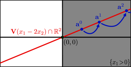
Figure 1. An illustration of a particular case of Example 4.7 where $(a_{1},a_{2})=(2,1)$. In blue are depicted the successive values $\mathbf{a}^{0},\mathbf{a}^{1},\dotsc$ of the variables $(x_{1},x_{2})$, in red is the real zero-set of the invariant ideal, and in gray the set $\mathcal{S}(0,x_{1})$ defined by the condition $x_{1}>0$.

Consider the elementary semi-algebraic loop from Appendix A. A direct study of the linear recursive sequence defined by the successive values $\mathbf{a}^{0},\mathbf{a}^{1},\dotsc$ of $(x_{1},x_{2})$ shows that this loop never terminates if, and only if $a_{1}>0$. Besides, $a_{2}x_{1}-a_{1}x_{2}=0$ is a polynomial invariant of this loop, and since every $\mathbf{a}^{j}$, for $j\geq 0$ must be on this line, it generates the whole invariant ideal. However, $\bm{V}(a_{2}x_{1}-a_{1}x_{2})\cap\mathbb{R}^{2}$ is not contained in $\mathcal{S}(0,x_{1})$ as shown in Figure 1.

5. Implementation and Experiments

In this section, we present an implementation of the algorithms presented in this paper and compare its performances with Polar (Moosbrugger et al., 2022), which is mainly based on (Amrollahi et al., 2022) for the case of unsolvable loops.

5.1. Implementation details

A prototype implementation of our algorithm in Macaulay2 (Grayson and Stillman, [n. d.]) for polynomial loops with fixed initial values is publicly available. The experiments are performed on a laptop equipped with a 4.8 GHz Intel i7 processor, 16 GB of RAM and 25 MB L3 cache. This prototype relies mainly on classic linear algebra routines and Gröbner bases computations available in Macaulay2. This makes the implementation quite direct from the pseudo-code presented here. We made slight modifications to these algorithms to speed up computations, based on observations from experiments, which we explain below.

We first observed that most of the time, for simple loops, all the candidate polynomials in $\mathcal{B}$, computed at step 6 of Algorithm 2, are actually polynomial invariants. Another observation, is that the smaller the dimension of the variety $X$ is, the faster Algorithm 1 computes polynomials defining $S_{(F,X)}$, for some polynomial map $F$. Hence, before checking them individually, we first test all elements of $\mathcal{B}$ at once. The collection of these polynomials defines a variety of smaller dimension than each individually, resulting in a potential speedup of up to 100 times (e.g., in Example 3.11).

Another observation is that the value $\binom{n+d}{d}$ for $M$ is a rough overestimate corresponding to the worst case scenario (when no polynomial invariant exists). Users can adjust this parameter according to the specific example. Notably, in most cases, if one linear equation $g(F^{k}(\mathbf{a}),\mathbf{y})$ is a linear combination of the others, the same applies to all subsequent equations $g(F^{l}(\mathbf{a}),\mathbf{y})$ for $k<l\leq\binom{n+d}{d}$.

5.2. Experimental results

In Tables 1 and 2, we compare our implementation of Algorithm 2 with the software Polar, which is based on (Amrollahi et al., 2022), for the case of unsolvable loops. The benchmarks include those presented in (Amrollahi et al., 2022) (with fixed initial values), as well as unsolvable loops in the last two rows, where Polar fails to find any polynomial invariant of degree less than 4.

Note that, unlike Algorithm 2, Polar can handle loops with arbitrary initial values. However, on these benchmarks, it only produces invariants of the form $f(\mathbf{x})-f(\mathbf{a})=0$, where $\mathbf{a}$ is the initial value, and $f\in\mathbb{Q}[\mathbf{x}]$. Thanks to Proposition 3.9, this can be achieved by our approach for a negligible additional cost, allowing us to determine whether such an invariant exists or not. A notable distinction is that our approach is global as we compute all possible polynomial invariants up to a specified degree, whereas Polar generates only a (possibly empty) subset of them. However, Polar can handle probabilistic loops, whereas ours is limited to deterministic ones.

In Table 1, we report quantitative data on the output of Algorithm 2 for various benchmarks (listed in the rows) and for generating polynomial invariants of degree $1,2,3,$ and $4$. Additionally, the column $d$ denotes the number of polynomials outputted by Algorithm 2, which is also the dimension of the associated truncated invariant ideal. Finally, in the column Polar, we report the number of polynomial invariants computed by Polar. In Table 2, we present the timings corresponding to the executions of Algorithm 2 as reported in Table 1. The timings are in seconds, and we chose a time limit of 360 seconds. In cases where Polar reaches this time limit (degree 4 for Yaghzhev9), we ensured that it does not terminate after 15 minutes or reach maximum recursion depth.

We remark that in Table 1, when there exists non-zero polynomial invariants, we almost always find more than Polar. For example, in the linear case, for Squares, we find the single invariant $1+x_{1}+x_{2}+x_{3}=0$ (see also Example 3.11). Additionally, for Yaghzev9, we find $x_{1}-x_{3}+x_{5}=0$, $x_{2}-x_{4}+x_{6}=0$, and $x_{8}-x_{7}-7=0$. Note also that for the case of Ex 10, Polar fails to find the following “general” invariant in terms of the initial values $(a_{1},a_{2},a_{3})$:

$(3a_{1}-a_{2}-4a_{3})^{2}(x_{1}+x_{2})-(3a_{1}-a_{2}-4a_{3})^{2}(x_{2}+x_{3})-9(a_{1}-a_{3})(x_{1}+x_{2})^{2}-16(a_{1}-a_{3})(x_{2}+x_{3})^{2}+24(a_{1}-a_{3})(x_{1}+x_{2})(x_{2}+x_{3})=0$.

However, for the Yagzhev9 and Yagzhev11 examples (with 9 and 11 variables, respectively), Polar handles degree 3, unlike our approach. Yet, both reach the fixed time limit at degree 4. Comparing timings in Table 2, our approach outperforms Polar for small degrees, but Polar demonstrates better performance for larger degrees and variables. However, since our method is complete, this increase in complexity is unavoidable.

In particular, even when the output is empty (i.e. $d=0$ in Table 2), or the same as Polar (the value of $d$ is the same in the column Polar), we can conclude that no additional (and linearly independent) polynomial invariant can be found.

Degree	1		2		3		4
Benchmark	d	Polar	d	Polar	d	Polar	d	Polar
Fib1	0	0	0	0	1	1	4	1
Fib2	0	0	0	0	1	1	TL	1
Fib3	0	0	0	0	1	1	4	1
Nagata	1	0	5	1	13	1	26	2
Yagzhev9	3	0	TL	3	TL	3	TL	TL
Yagzhev11	0	0	0	0	TL	1	TL	TL
Ex 9	0	0	0	0	3	1	11	1
Ex 10	0	0	2	0	8	0	19	0
Squares (Ex 3.11)	1	0	5	0	13	0	26	0

TL = Timeout (360 seconds);  bold: new invariants found

Table 1. Data on outputs of Algorithm 2 and Polar

Degree	1		2		3		4
Benchmark	Ours	Polar	Ours	Polar	Ours	Polar	Ours	Polar
Fib1	0.014	0.2	0.046	0.32	0.17	0.68	37.07	1.58
Fib2	0.017	0.23	0.056	0.46	12.62	1.18	TL	3.69
Fib3	0.013	0.21	0.056	0.4	0.225	1.18	7.11	3.82
Nagata	0.014	0.25	0.057	0.55	0.09	1.21	0.19	2.84
Yagzhev9	1.46	0.43	TL	5.2	TL	131.5	TL	TL
Yagzhev11	0.075	0.45	61.4	6.83	TL	359	TL	TL
Ex 9	0.016	0.28	0.06	0.64	0.19	2.38	0.55	11.5
Ex 10	0.014	0.51	0.058	0.7	0.16	1.21	0.45	2.3
Squares (Ex 3.11)	0.0151	0.5	0.085	0.67	0.25	1.15	1.6	2.25

TL = Timeout (360 seconds);

Table 2. Timings for Algorithm 2 and Polar, in seconds

Appendix A Examples and Benchmarks

• $$Squares$$
  $(x_{1},x_{2},x_{3})=(-1,-1,1)$ while true do      $\begin{pmatrix}x_{1}\\ x_{2}\\ x_{3}\end{pmatrix}\longleftarrow\begin{pmatrix}2x_{1}+x_{2}^{2}+x_{3}\\ 2x_{2}-x_{2}^{2}+2x_{3}\\ 1-x_{3}\end{pmatrix}$ end while
  

• $$Fib1$$
  $(x_{1},x_{2},x_{3})=(2,1,1)$ while true do      $\begin{pmatrix}x_{1}\\ x_{2}\\ x_{3}\end{pmatrix}\longleftarrow\begin{pmatrix}x_{2}\\ x_{3}\\ 2x_{2}x_{3}-x_{1}\end{pmatrix}$ end while
  

• $$Fib2$$
  $(x_{1},x_{2},x_{3})=(3,-2,1)$ while true do      $\begin{pmatrix}x_{1}\\ x_{2}\\ x_{3}\end{pmatrix}\longleftarrow\begin{pmatrix}x_{2}\\ 2x_{1}x_{3}-x_{2}\\ 4x_{1}x_{2}x_{3}-2x_{1}^{2}-2x_{2}^{2}+1\end{pmatrix}$ end while
  

• $$Example\mathrm{\hspace{0.17em}9}$$
  $(x_{1},x_{2},x_{3})=(3,-1,2)$ while true do      $\begin{pmatrix}x_{1}\\ x_{2}\\ x_{3}\end{pmatrix}\longleftarrow\begin{pmatrix}x_{1}+x_{3}^{2}+1\\ x_{2}-x_{3}^{2}\\ x_{3}+(x_{1}+x_{2})^{2}\end{pmatrix}$ end while
  

• $$Fib3$$
  $(x_{1},x_{2},x_{3})=(2,-1,1)$ while true do      $\begin{pmatrix}x_{1}\\ x_{2}\\ x_{3}\end{pmatrix}\longleftarrow\begin{pmatrix}1+x_{1}+x_{2}+x_{1}x_{2}-x_{3}\\ x_{1}\\ x_{2}\end{pmatrix}$ end while
  

• $$Example\mathrm{\hspace{0.17em}10}$$
  $(x_{1},x_{2},x_{3})=(-1,2,1)$ while true do      $\begin{pmatrix}x_{1}\\ x_{2}\\ x_{3}\end{pmatrix}\longleftarrow\begin{pmatrix}10x_{1}-8x_{3}+(x_{1}+x_{2})^{2}\\ 2x_{2}-(x_{1}+x_{2})^{2}\\ 6x_{1}-4x_{3}+(x_{1}+x_{2})^{2}\end{pmatrix}$ end while
  

• $$Nagata$$
  $(x_{1},x_{2},x_{3})=(3,-2,5)$ while true do      $\begin{pmatrix}x_{1}\\ x_{2}\\ x_{3}\end{pmatrix}\longleftarrow\begin{pmatrix}x_{1}-2(x_{1}x_{3}+x_{2}^{2})x_{2}-(x_{1}x_{3}+x_{2}^{2})^{2}x_{3}\\ x_{2}+(x_{1}x_{3}+x_{2}^{2})x_{3}\\ x_{3}\end{pmatrix}$ end while
  

• $$Yagzhev9$$
  $(x_{1},\ldots,x_{9})=(2,-3,1,4,-1,7,-4,3,2)$ while true do      $\begin{pmatrix}x_{1}\\ x_{2}\\ x_{3}\\ x_{4}\\ x_{5}\\ x_{6}\\ x_{7}\\ x_{8}\\ x_{9}\end{pmatrix}\longleftarrow\begin{pmatrix}x_{1}+x_{1}x_{7}x_{9}+x_{2}x_{9}^{2}\\ x_{2}-x_{1}x_{7}^{2}-x_{2}x_{7}x_{9}\\ x_{3}+x_{3}x_{7}x_{9}+x_{4}x_{9}^{2}\\ x_{4}-x_{3}x_{7}^{2}-x_{4}x_{7}x_{9}\\ x_{5}+x_{5}x_{7}x_{9}+x_{6}x_{9}^{2}\\ x_{6}-x_{5}x_{7}^{2}-x_{6}x_{7}x_{9}\\ x_{7}+(x_{1}x_{4}-x_{2}x_{3})x_{9}\\ x_{8}+(x_{3}x_{6}-x_{4}x_{5})x_{9}\\ \big{(}x_{9}+(x_{1}x_{4}-x_{2}x_{3})x_{8}\\ -(x_{3}x_{6}+x_{4}x_{5})x_{7}\big{)}\end{pmatrix}$ end while
  

• $$Yagzhev11$$
  $(x_{1},\ldots,x_{11})=(3,-1,2,1,-5,-1,3,4,-1,3,2)$ while true do      $\begin{pmatrix}x_{1}\\ x_{2}\\ x_{3}\\ x_{4}\\ x_{5}\\ x_{6}\\ x_{7}\\ x_{8}\\ x_{9}\\ x_{10}\\ x_{11}\end{pmatrix}\longleftarrow\begin{pmatrix}x_{1}-x_{3}x_{10}^{2}\\ x_{2}-x_{3}x_{11}^{2}\\ x_{3}+x_{1}x_{11}^{2}-x_{2}x_{10}^{2}\\ x_{4}-x_{6}x_{10}^{2}\\ x_{5}-x_{6}x_{11}^{2}\\ x_{6}+x_{4}x_{11}^{2}-x_{5}x_{10}^{2}\\ x_{7}-x_{9}x_{10}^{2}\\ x_{8}-x_{9}x_{11}^{2}\\ x_{9}+x_{7}x_{11}^{2}-x_{8}x_{10}^{2}\\ x_{10}-\det(A)\\ x_{11}-x_{10}^{3}\end{pmatrix}$ end whilewhere $A=\begin{pmatrix}x_{1}&x_{2}&x_{3}\\ x_{4}&x_{5}&x_{6}\\ x_{7}&x_{8}&x_{9}\end{pmatrix}$
  

• $$Semi\text{-}algebraic$$
  $(x_{1},x_{2})=(a_{1},a_{2})$ while $x_{1}>0$ do      $\begin{pmatrix}x_{1}\\ x_{2}\end{pmatrix}\longleftarrow\begin{pmatrix}2x_{1}\\ 2x_{2}\end{pmatrix}$ end while

References

• (1)
• Amrollahi et al. (2022) Daneshvar Amrollahi, Ezio Bartocci, George Kenison, Laura Kovács, Marcel Moosbrugger, and Miroslav Stankovič. 2022. Solving invariant generation for unsolvable loops. In International Static Analysis Symposium. Springer, 19–43.
• Amrollahi et al. (2023) Daneshvar Amrollahi, Ezio Bartocci, George Kenison, Laura Kovács, Marcel Moosbrugger, and Miroslav Stankovič. 2023. (Un) Solvable Loop Analysis. arXiv preprint arXiv:2306.01597 (2023).
• Baake et al. (1993) Michael Baake, Uwe Grimm, and Dieter Joseph. 1993. Trace maps, invariants, and some of their applications. International Journal of Modern Physics B 7, 06n07 (1993), 1527–1550.
• Basu et al. (2006) Saugata Basu, Richard Pollack, and Marie-Françoise Roy. 2006. Algorithms in Real Algebraic Geometry (2nd revised and extended 2016 ed.). Springer International Publishing. https://doi.org/10.1007/3-540-33099-2
• Berthomieu et al. (2021) Jérémy Berthomieu, Christian Eder, and Mohab Safey El Din. 2021. Msolve: A library for solving polynomial systems. In Proceedings of the 2021 on International Symposium on Symbolic and Algebraic Computation. 51–58.
• Bochnack et al. (1998) Jan Bochnack, Michel Coste, and Marie-Françoise Roy. 1998. Real Algebraic Geometry (1st ed.). Ergebnisse der Mathematik und ihrer Grenzgebiete, Vol. 3. Springer-Verlag, Berlin, Heidelberg. https://doi.org/10.1007/978-3-642-85463-2
• Chatterjee et al. (2020) Krishnendu Chatterjee, Hongfei Fu, Amir Kafshdar Goharshady, and Ehsan Kafshdar Goharshady. 2020. Polynomial invariant generation for non-deterministic recursive programs. In Proceedings of the 41st ACM SIGPLAN Conference on Programming Language Design and Implementation. 672–687.
• Cox et al. (2013) David Cox, John Little, and Donal O’Shea. 2013. Ideals, varieties, and algorithms: an introduction to computational algebraic geometry and commutative algebra. Springer Science & Business Media.
• Cyphert and Kincaid (2024) John Cyphert and Zachary Kincaid. 2024. Solvable Polynomial Ideals: The Ideal Reflection for Program Analysis. Proceedings of the ACM on Programming Languages 8, POPL (2024), 724–752.
• de Oliveira et al. (2016) Steven de Oliveira, Saddek Bensalem, and Virgile Prevosto. 2016. Polynomial invariants by linear algebra. In Automated Technology for Verification and Analysis: 14th International Symposium, ATVA 2016, Chiba, Japan, October 17-20, 2016, Proceedings 14. Springer, 479–494.
• de Oliveira et al. (2017) Steven de Oliveira, Saddek Bensalem, and Virgile Prevosto. 2017. Synthesizing invariants by solving solvable loops. In International Symposium on Automated Technology for Verification and Analysis. Springer, 327–343.
• Eder and Faugère (2017) Christian Eder and Jean-Charles Faugère. 2017. A survey on signature-based algorithms for computing Gröbner bases. Journal of Symbolic Computation 80 (2017), 719–784.
• Floyd (1993) Robert W Floyd. 1993. Assigning meanings to programs. In Program Verification: Fundamental Issues in Computer Science. Springer, 65–81.
• Goharshady et al. (2023) Amir Kafshdar Goharshady, S Hitarth, Fatemeh Mohammadi, and Harshit Jitendra Motwani. 2023. Algebro-geometric Algorithms for Template-based Synthesis of Polynomial Programs. Proceedings of the ACM on Programming Languages 7, OOPSLA1 (2023), 727–756.
• Grayson and Stillman ([n. d.]) Daniel R. Grayson and Michael E. Stillman. [n. d.]. Macaulay2, a software system for research in algebraic geometry. Available at http://www2.macaulay2.com.
• Hrushovski et al. (2018) Ehud Hrushovski, Joël Ouaknine, Amaury Pouly, and James Worrell. 2018. Polynomial invariants for affine programs. In Proceedings of the 33rd Annual ACM/IEEE Symposium on Logic in Computer Science. 530–539.
• Hrushovski et al. (2023) Ehud Hrushovski, Joël Ouaknine, Amaury Pouly, and James Worrell. 2023. On strongest algebraic program invariants. J. ACM 70, 5 (2023), 1–22.
• Karr (1976) Michael Karr. 1976. Affine relationships among variables of a program. Acta Informatica 6 (1976), 133–151.
• Kauers and Zimmermann (2008) Manuel Kauers and Burkhard Zimmermann. 2008. Computing the algebraic relations of C-finite sequences and multisequences. Journal of Symbolic Computation 43, 11 (2008), 787–803.
• Kempf (1993) G. Kempf. 1993. Algebraic Varieties. Cambridge University Press. https://doi.org/10.1017/CBO9781107359956
• Kovács (2008) Laura Kovács. 2008. Reasoning algebraically about p-solvable loops. In International Conference on Tools and Algorithms for the Construction and Analysis of Systems. Springer, 249–264.
• Kovács (2023) Laura Kovács. 2023. Algebra-Based Loop Analysis. In Proceedings of the 2023 International Symposium on Symbolic and Algebraic Computation. 41–42.
• Manna and Pnueli (2012) Zohar Manna and Amir Pnueli. 2012. Temporal verification of reactive systems: safety. Springer Science & Business Media.
• Mayr and Meyer (1982) E. Mayr and A. Meyer. 1982. The complexity of the word problem for commutative semi-groups and polynomial ideals. Advances in Mathematics 46 (1982), 305–329. https://doi.org/10.1016/0001-8708(82)90035-9
• Moosbrugger et al. (2022) Marcel Moosbrugger, Miroslav Stankovic, Ezio Bartocci, and Laura Kovács. 2022. This is the moment for probabilistic loops. Proc. ACM Program. Lang. 6, OOPSLA2 (2022), 1497–1525. https://doi.org/10.1145/3563341
• Moreno Socias (1992) Guillermo Moreno Socias. 1992. Length of Polynomial Ascending Chains and Primitive Recursiveness. MATHEMATICA SCANDINAVICA 71 (Jun. 1992), 181–205. https://doi.org/10.7146/math.scand.a-12421
• Müller-Olm and Seidl (2004a) Markus Müller-Olm and Helmut Seidl. 2004a. Computing polynomial program invariants. Inform. Process. Lett. 91, 5 (2004), 233–244.
• Müller-Olm and Seidl (2004b) Markus Müller-Olm and Helmut Seidl. 2004b. A note on Karr’s algorithm. In International Colloquium on Automata, Languages, and Programming. Springer, 1016–1028.
• Pastuszak (2020) Grzegorz Pastuszak. 2020. Ascending chains of ideals in the polynomial ring. Turkish Journal of Mathematics 44, 6 (2020), 2652–2658. https://doi.org/10.3906/mat-1904-61
• Putinar (1993) Mihai Putinar. 1993. Positive Polynomials on Compact Semi-algebraic Sets. Indiana University Mathematics Journal 42, 3 (1993), 969–984. https://doi.org/stable/24897130
• Roberts and Baake (1994) John AG Roberts and Michael Baake. 1994. Trace maps as 3D reversible dynamical systems with an invariant. Journal of statistical physics 74, 3-4 (1994), 829–888.
• Rodríguez-Carbonell and Kapur (2004) Enric Rodríguez-Carbonell and Deepak Kapur. 2004. Automatic generation of polynomial loop invariants: Algebraic foundations. In Proceedings of the 2004 international symposium on Symbolic and algebraic computation. 266–273.
• Rodríguez-Carbonell and Kapur (2007a) Enric Rodríguez-Carbonell and Deepak Kapur. 2007a. Automatic generation of polynomial invariants of bounded degree using abstract interpretation. Science of Computer Programming 64, 1 (2007), 54–75.
• Rodríguez-Carbonell and Kapur (2007b) Enric Rodríguez-Carbonell and Deepak Kapur. 2007b. Generating all polynomial invariants in simple loops. Journal of Symbolic Computation 42, 4 (2007), 443–476.
• Shafarevich and Reid (1994) Igor Rostislavovich Shafarevich and Miles Reid. 1994. Basic algebraic geometry. Vol. 1. Springer.
• Von Zur Gathen and Gerhard (2013) Joachim Von Zur Gathen and Jürgen Gerhard. 2013. Modern computer algebra. Cambridge university press.