Particle transport based study of nucleation in a ferromagnetic three-state spin system with conservative dynamics

Abstract

We pose the problem of metastability for a three–state spin system with conservative dynamics. We consider the Blume–Capel model with the Kawasaki dynamics, we prove that, in a particular region of the parameter plane, the metastable state is the unique homogeneous minus state, and we estimate the exit time. To achieve our goal we have to solve several variational problems in the configuration space which result to be particularly involved, due to complicated structure of the trajectories. They key ingredient is the control of the energy differences between the configurations crossed when a spin is transported from the boundary to an internal site of the lattice through a completely arbitrary mixture of the three–state spin species. To master these mechanisms we have introduced a new approach based on the transport of spins along nearest neighbor connected regions of the lattice with constant spin configuration. This novel approach goes beyond the Blume–Capel model and can be used for the study of more general multi–state spin models.

Keywords: Kawasaki dynamics, multi–state systems, metastability, nucleation, low temperature dynamics

Bozza:

1 Introduction

Metastable states are very common in nature and are observed in several physical systems. Their mathematical description is a challenging task that, in the last decades, has given rise to different approaches and has been attacked from different angles. For a systematic discussion of the literature related to the so–called pathwise and potential–theoretic approaches we refer to the monografies [35, 11] and to the review [14]. For the more recent trace method we refer, for instance, to [8].

The pertinent literature is characterized by the alternation of abstract studies [9, 31], in which general theories are proposed or refined, and applied ones in which the behavior of special models is discussed. The latter, beside their interest due to specific novel applications, see, e.g., [1, 22] for the 3D Ising model, [2, 4] for applications to non-square lattices, and [3] for the Ising model on a family of finite networks, play an important role in suggesting possible progresses of the general theories.

This is a paper of the second type in which we investigate the metastable behavior of the Blume–Capel lattice spin model [10, 25] under the Kawasaki dynamics [26] in finite volume and in the zero temperature limit. The model is characterized by the fact that the lattice spin variables can assume the three states minus, zero, and plus, and the Hamiltonian is ferromagnetic. Moreover, the Kawasaki dynamics, reversible with respect to the Gibbs measure, allows in the bulk only the swaps between neighboring spins. This is a particularly challenging problem since it combines the difficulties due to the three state character of the spins and those due to the conservative character of the dynamics.

Before entering into the details of our work, we review briefly the papers in which the metastable behavior of the Blume–Capel model with the Glauber non–conservative dynamics has been investigated. The first results were published in [18] in finite volume and in the zero-temperature limit. In [16, 27, 17] a peculiar version of the model, for which there exist two non–degenerate in energy metastable states, is studied. The infinite volume regime is considered in [32, 28]. We mention, also, that in the interesting paper [19], this model has been studied at finite temperature with non–rigorous methods, such as Monte Carlo simulations and transfer matrix approaches. Moreover, in different regimes, thanks to its great ductility, the Blume–Capel model and its generalizations have been recently used to study the pattern formation in three–components mixtures of polymers and solvent [29, 33, 30]. In all these studies the model is defined on a torus, namely, periodic boundary conditions are considered.

In our recent work [15] we attack this model with zero boundary conditions and discuss the metastability scenario on the parameter plane, comparing it with what was already known for periodic boundary conditions. In particular, we prove that, depending on the choice of the parameters, the system can exhibit both homogeneous and heterogeneous nucleation triggered by the boundary. Beside its intrinsic interest, [15] is a sort of prequel of the present paper in which we study the Kawasaki case where zero boundary conditions are natural for modelling the exchange of particles between the system and the reservoir.

The rigorous study of metastability for a Kawasaki dynamics has been a challenging problem from the very beginning: the number of particles is indeed conserved in the interior of a finite box, so that during the nucleation particles must travel between the droplet and the boundary of the box, which causes several mathematical complications. A first simplified local 2D model for a Ising lattice gas was introduced in [24], where only the particles inside a finite box were considered for the interaction, while the particles outside evolved via non-interacting random walks. The removal of the interaction outside the finite box allowed the mathematical control of the gas of particles, and it was consistent with the physical picture of an ideal gas approximation of a low density gas in the limit in which the temperature tends to zero.

The crucial point was indeed that at low density, say proportional to the exponential of minus the inverse of the temperature, the gas outside the finite box could be treated as a reservoir that creates particles with rate equal to the small density at sites on the interior boundary of the finite box and annihilates particles with rate one at the external boundary sites.

The local dynamics results in [24] for the Ising lattice gas were extended to the 3D case in [22], with the sharp asymptotics given in [12], and to the anisotropic Ising lattice gas in [34, 7, 5, 6].

Moreover, the case of volumes growing moderately fast as the temperature decreases was first studied in [20] by using the pathwise approach, then in [13] with the use of the potential theoretic approach, and finally in [21] with the trace method. All these results have been derived for two spin classical lattice gases with Kawasaki dynamics.

To our knowledge, [23] is the sole paper in which the metastable behavior of a three state system with a conservative dynamics has been approached. In that paper a swap dynamics is considered for a model with three state site variables (zero, one, and two) in which direct swaps between the states one and two are not allowed. Moreover, the Hamiltonian is not ferromagnetic in the sense that it promotes the interface between states one and two, with respect to all other possible bond configurations, which are all alike; thus the single interface one–two is favored with respect to all the others. This yields in a chessboard–like stable state with the sites of the even and odd sublattices occupied, respectively, by state one and two or viceversa.

In the present paper, in contrast with [23], we approach the Blume–Capel model with the Kawaski dynamics allowing swaps between spins of any value. Moreover, the ferromagnetic interaction favors the three type of bonds between sites sharing the same spin, whereas the bonds between different spins are not alike, but pay different energy costs, indeed, the minus–plus bond costs four times the zero–minus and the zero–plus bonds. This fact complicates the study of the model: due to the interface energy cost hierarchy, plus structures cannot grow freely inside minus regions, but must always be protected by a thin layer of zeros. In other words, in order to perform changes of the system configuration in which a plus structure grows inside a minus background, before substituting bulk pluses with minuses, it is necessary to let zeros populate the bulk to avoid direct interfaces between minus and plus regions. Controlling these mechanisms becomes utterly difficult in the case of conservative dynamics, since the spins cannot be locally created, as it is the case for non–conservative ones, but they must first enter the lattice at its boundary and then be transported through the bulk to the spot where they are needed.

The complications that arise are due to the necessity to control energy differences along path of configurations corresponding to the transport of one spin (either minus, zero, or plus) along the lattice through a completely general mixture of the three spin species. In this paper we manage these mechanisms by means of new techniques based on the idea that spins are transported through the lattice along regions made of nearest neighbor connected sites with constant spin value. It is important to stress that the energy cost associated to the transport of spins along the lattice is controlled in Lemma 3.4 which is susceptible of being extended to more general multi–spin models, such as a generalized Potts model with different interface energy costs, see Lemma 5.15. Thus, the results discussed in this paper can open the way to new studies of conservative dynamics for general multi–state spin systems.

Coming back to this work, we focus on a region of the parameter plane where we are able to prove the uniqueness of the metastable state (the homogeneous minus configuration) and to study the transition to the unique stable configuration (the homogeneous plus state), that is to say, to the absolute minimum of the energy. This is achieved in the framework of the pathwise approach as formulated in [31] by solving two model dependent problems: call the stability level of a configuration the minimal energy barrier that has to be overcome by a path connecting such a configuration to any other at lower energy, then compute the stability level of the homogeneous minus configuration and show that the stability level of any other configuration is strictly smaller. These two problems are addressed in the literature respectively as the optimal path and the recurrence problem.

Due to the very intricated structure of the trajectories of our three–state conservative model, we solve a weaker version of the optimal path problem, that is to say, we do not compute exactly the stability level of the homogeneous minus configuration, but we show that it belongs to a closed interval. As for the recurrence property, we show that the stability level of all other configurations is smaller than the infimum of this interval. This allows us to prove that the homogeneous minus configuration is the metastable state and to prove an estimate for the exit time from it with an uncertainty related to the width of the interval. We remark that, due to the uncertainty on the value of the stability level of the homogeneous minus configuration, it is natural to use the pathwise approach, since the other methods need a more detailed control of the energy landscape, i.e., of the minimizers of the Dirichlet form associated to the dynamics.

The paper is organized as follows. In Section 2 we introduce the model and state our main results. Section 3 is devoted to the proof of the theorems which are based on the key Lemma 3.4 about the particle transport. The proofs of the more technical lemmas are reported in Section 4. In Section 5 we summarize our conclusions, propose a generalization of our key lemma, and discuss its potential applications to general multi–state spin systems.

2 Model and results

In this section we introduce the Blume–Capel model with the Kawasaki dynamics and state our main results.

2.1 The lattice

We consider the set $\mathbb{Z}^{2}$ embedded in $\mathbb{R}^{2}$ and call sites its elements. We will denote by $\{e_{1},e_{2}\}$ the canonical base of $\mathbb{R}^{2}$ and we will often address to the direction $1$ (resp. $2$) as the horizontal (resp. vertical) direction. Given two sites $x,x^{\prime}\in\mathbb{Z}^{2}$ we let $|x-x^{\prime}|$ be their Euclidian distance. Given $x\in\mathbb{Z}^{2}$, we say that $x^{\prime}\in\mathbb{Z}^{2}$ is a nearest neighbor of $x$ if and only if $|x-x^{\prime}|=1$. Pairs of neighboring sites will be called bonds. A set $X\subset\mathbb{Z}^{2}$ is connected if and only if for any $x\neq x^{\prime}\in X$ there exists a sequence $x_{1},x_{2},\dots,x_{n}$ of sites of $X$ such that $x_{1}=x$, $x_{n}=x^{\prime}$, and $x_{k}$ and $x_{k+1}$ are nearest neighbors for any $k=1,\dots,n-1$.

Given $X\subset\mathbb{Z}^{2}$ we call internal boundary $\partial^{-}X$ of $X$ the set of sites in $X$ having a nearest neighbor outside $X$. The interior or bulk of $X$ is the set $X\setminus\partial^{-}X$, namely, the set of sites of $X$ having four nearest neighbors inside $X$. We call external boundary $\partial^{+}X$ of $X$ the set of sites in $\mathbb{Z}^{2}\setminus X$ having a nearest neighbor inside $X$.

A column, resp. a row, of $\mathbb{Z}^{2}$ is a sequence of $L$ connected sites of $\Lambda$ such that the line joining them is parallel to the vertical, resp. horizontal, axis.

A set $R\subset\mathbb{Z}^{2}$ is called a rectangle (resp. square) of $\mathbb{Z}^{2}$ if the union of the closed unit squares of $\mathbb{R}^{2}$ centered in the sites of $R$ with sides parallel to the axes of $\mathbb{Z}^{2}$ is a rectangle (resp. a square) of $\mathbb{R}^{2}$. The sides of a rectangle of $\mathbb{Z}^{2}$ are the four maximal connected subsets of its internal boundary (note that they lie on straight lines parallel to the axes of $\mathbb{Z}^{2}$). The length of one side of a rectangle of $\mathbb{Z}^{2}$ is the number of sites belonging to the side itself. A quasi–square is a rectangle with side lengths equal to $n$ and $n+1$, with $n$ an integer greater than or equal to one.

We equip $\mathbb{Z}^{2}$ with a directed graph structure by considering the set of directed edges $(x\to y)$ where $\{x,y\}\subset\mathbb{Z}^{2}$ such that $|x-y|=1$.

2.2 The configuration space

Let $\Lambda:=\{0,...,L+1\}^{2}\subset\mathbb{Z}^{2}$ be a finite square with fixed side length $L+2$ and denote its interior by $\Lambda_{0}:=\Lambda\setminus\partial^{-}\Lambda=\{1,...,L\}^{2}$. Remark that $\partial^{+}\Lambda_{0}$ is not equal to $\partial^{-}\Lambda$, since the four corner sites of $\Lambda$ belong to $\partial^{-}\Lambda$, but not to $\partial^{+}\Lambda_{0}$. We denote by $E\subset\Lambda\times\Lambda$ the collection of all the directed edges $(x\to y)$ such that $x,y\in\Lambda$ and $E_{0}:=\{(x\to y)\in E|x,y\in\Lambda_{0}\}$ the set of oriented edges with both vertices in $\Lambda_{0}$.

With each $x\in\Lambda$ we associate a spin variable $\sigma(x)\in\{-1,0,+1\}$. Moreover, we let $\mathcal{X}:=\{{-1,0,+1}\}^{\Lambda}$ be the configuration space and $\hat{\mathcal{X}}:=\{\sigma\in\mathcal{X}\,|\,\sigma(x)=0\,\forall x\in\partial^{-}\Lambda\}$ be the set of configurations with spin $0$ associated to the sites in the internal boundary of $\Lambda$.

Given a configuration $\sigma\in\mathcal{X}$, if $\sigma(x)=0$ we say that the site is empty, otherwise, if $\sigma(x)=+1$ (resp. $\sigma(x)=-1$), we say that it is occupied by a particle with spin plus (resp. minus).

Given a configuration $\sigma\in\mathcal{X}$ and a set $A\subseteq\Lambda_{0}$, we denote $\sigma_{|A}$ by $\sigma_{A}$. Finally, given $s\in\{-1,0,+1\}$ and $A\subseteq\Lambda_{0}$, we denote by $s_{A}$ the homogeneous configuration $\sigma\in\{-1,0,+1\}^{A}$ with spin equal to $s$ for any site in $A$. The symbols ${\boldsymbol{-1}}$, ${\boldsymbol{0}}$, ${\boldsymbol{+1}}$ denote, respectively, the configurations with spins zero in $\partial^{+}\Lambda_{0}$ and spins $-1$, $0$, and $+1$ in $\Lambda_{0}$, namely the homogeneous configuration in the interior of $\Lambda$.

2.3 Hamiltonian of the model and assumptions on its parameters

The Blume–capel Hamiltonian is defined in terms of three real parameters $J>0$, $\lambda$, and $h$, respectively called coupling constant, chemical potential, and magnetic field. It is also convenient to set

$$\Delta^{p}=4J-(\lambda+h)\;\;\textrm{ and }\;\;\Delta^{m}=4J-(\lambda-h).$$ (2.1)

For any $s\in\{-1,+1\}$, we define

$$\Delta_{s}=\frac{1-s}{2}\Delta^{m}+\frac{1+s}{2}\Delta^{p}.$$ (2.2)

We now introduce a particular version of the Hamiltonian of the Blume–Capel model which is well suited to treat the particle exchange between the bulk and the boundary:

$$H(\sigma)=H_{0}(\sigma)+\Delta^{p}{\sum_{i\in\partial^{+}\Lambda_{0}}}{\mathbf{1}}_{\{\sigma(i)=+1\}}+\Delta^{m}{\sum_{i\in\partial^{+}\Lambda_{0}}}{\mathbf{1}}_{\{\sigma(i)=-1\}}$$ (2.3)

where

$$H_{0}(\sigma)=\frac{J}{2}\sum_{\genfrac{}{}{0.0pt}{}{i,j\in\Lambda_{0}:}{|i-j|=1}}[\sigma(i)-\sigma(j)]^{2}+J\sum_{i\in\partial^{-}\Lambda_{0}}\sum_{\genfrac{}{}{0.0pt}{}{j\in\mathbb{Z}^{2}\setminus\Lambda_{0}:}{|i-j|=1}}[\sigma(i)]^{2}-\lambda\sum_{i\in\Lambda_{0}}\sigma(i)^{2}-h\sum_{i\in\Lambda_{0}}\sigma(i).$$ (2.4)

Note that if in a configuration $\sigma$ a spin zero surrounded by zeros is changed to plus or minus the value of the energy $H_{0}$ increases precisely of $\Delta^{p}$ and $\Delta^{m}$, respectively. Thus, these two quantities can be interpreted as the energy cost of a plus and a minus spin in the sea of zeros.

We note that if $\sigma$ is a configuration such that the external boundary of $\Lambda_{0}$ is filled with zero spins, then $H(\sigma)=H_{0}(\sigma)$. It is interesting to remark that the function $H_{0}$ in (2.4) is precisely the Hamiltonian of the Blume–Capel model that has been used in [15] to study the Blume–Capel model with Glauber dynamics in the case of zero boundary conditions. Here, we consider the Hamiltonian (2.3) to take into account the energy cost of particles that must be created in the boundary $\partial^{+}\Lambda_{0}$ to run the Kawasaki dynamics mimicking the presence of an external gas with fixed density of plus and minus spins.

The equilibrium state of the Blume–Capel model with zero boundary condition on $\Lambda$ and at temperature $1/\beta$, with $\beta$ a positive real number, is described by the Gibbs measure

$$\mu_{\beta}(\sigma)=\frac{e^{-\beta H(\sigma)}}{Z_{\beta}},$$ (2.5)

where $Z_{\beta}:=\sum_{\eta\in\mathcal{X}}e^{-\beta H(\eta)}$ is the partition function.

In the sequel we shall discuss the metastable behavior of the Blume–Capel model, but, to do so, we will rely on the following assumptions on the parameters (see, also, Figure 1):

$$i) \,\lambda>0\;\textup{ and }\;\frac{\lambda}{2}<h<\min\Big{\{}\lambda,\frac{1}{3}J-\lambda\Big{\}}$$ (2.6)

$$ii) \,\lambda<\frac{4J(1-h/\lambda)}{h/\lambda(1+h/\lambda)}\Bigg{[}-\frac{2(1-2h/\lambda)}{h/\lambda}+\sqrt{\frac{64}{1+h/\lambda}-\frac{22}{h/\lambda}-6}\Bigg{]}^{-1}\;\;\textup{ for }\;\;\frac{h}{\lambda}>\frac{1}{3}(9-4\sqrt{3})$$ (2.7)

$$iii) \,L>\Big{(}\frac{2J}{\lambda-h}\Big{)}^{3}\;\textup{ and }\;\frac{2J}{\lambda+h},\,\frac{2J}{\lambda-h},\,\frac{2J+\lambda-h}{2h}\;\;\textup{ are not integers}.$$ (2.8)

Condition (2.6) implies that $\Delta^{p}$ and $\Delta^{m}$ are both positive and will be also used in the proof of Theorem 2.1. Conditions (2.7)–(2.8) are more technical, in particular (2.7) is related to the uncertainty on the computation of the stability level of the configuration ${\boldsymbol{-1}}$, as mentioned already in the introduction (see, also, Theorem 2.2 and the way in which it is used in Section 3.7). Note that the above conditions are not completely independent one from each other, indeed, in the case $\xi$ much larger than $(9-4\sqrt{3})/3$ the condition (2.7) implies the requirements assumed in (2.6) on $h$.

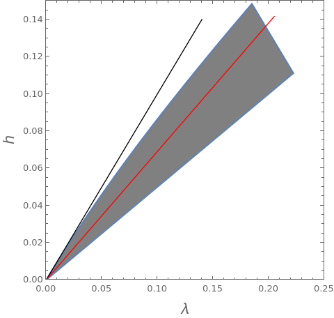
Figure 1: Region of the parameters space compatible with assumptions (2.6)–(2.8) for $J=1$. The red and the black lines have, respectively, slope $(9-4\sqrt{3})/3$ and $1$.

We close this section by remarking that a simple computation yields that the Hamiltonian (2.3) can be rewritten as follows

$$H(\sigma)=-J\!\!\!\!\sum_{(x\to y)\in E_{0}}\!\!\!\!\!{\mathbf{1}}_{\{\sigma({x})\sigma({y})=+1\}}+J\!\!\!\!\sum_{(x\to y)\in E_{0}}\!\!{\mathbf{1}}_{\{\sigma({x})\sigma({y})=-1\}}+\Delta^{p}\!\!\!\!\!\!{\sum_{x\in\Lambda_{0}\cup\partial^{+}\Lambda_{0}}}\!\!\!\!{\mathbf{1}}_{\{\sigma(x)=+1\}}+\Delta^{m}\!\!\!\!\!\!{\sum_{x\in\Lambda\cup\partial^{+}\Lambda_{0}}}\!\!\!\!{\mathbf{1}}_{\{\sigma(x)=-1\}}.$$ (2.9)

This is an interesting expression pointing out that the interaction takes effect only inside $\Lambda_{0}$ and that the binding energy associated to a positive bond is $-J<0$ (respectively, $J>0$ for a negative bond).

2.4 Energy landscape

The energy difference (energy cost) associated with each possible swap between two particles of different type plays a crucial role in the proof of several results.

Given $\sigma\in\mathcal{X}$, we well consider the following transformations: we denote by $\sigma^{(x,y)}$ the configuration obtained by swapping the values of the spins at sites $x$ and $y$ in $\sigma$, by $\sigma^{(x;0)}$ the configuration obtained from $\sigma$ by replacing the value of the spin at site $x$ with $0$, and by $\sigma^{(x;s)}$ the configuration obtained from $\sigma$ by replacing the value of the spin at site $x$ with $s\in\{-1,+1\}$, more precisely, we set

$$\sigma^{(x,y)}(z)=\left\{\begin{array}[]{ll}\!\sigma(z)&\!\!\textrm{if }z\neq x,y\\ \!\sigma(y)&\!\!\textrm{if }z=x\\ \!\sigma(x)&\!\!\textrm{if }z=y,\\ \end{array}\right.\;\;\sigma^{(x;0)}(z)=\left\{\begin{array}[]{ll}\!\sigma(z)&\!\!\textrm{if }z\neq x\\ \!0&\!\!\textrm{if }z=x,\end{array}\right.\;\;\sigma^{(x;s)}(z)=\left\{\begin{array}[]{ll}\!\sigma(z)&\!\!\textrm{if }z\neq x\\ \!s&\!\!\textrm{if }z=x.\end{array}\right.$$ (2.10)

In order to express conveniently the energy differences, we introduce the following energy cost functions. Let $\sigma\in\mathcal{X}$ and $x\in\Lambda$, we set

$$D_{x}(\sigma):=\sum_{\begin{subarray}{c}y\in\Lambda\\ |x-y|=1\end{subarray}}\textbf{1}_{\{\sigma(y)\sigma(x)=+1\}}\,-\sum_{\begin{subarray}{c}y\in\Lambda\\ |x-y|=1\end{subarray}}\textbf{1}_{\{\sigma(y)\sigma(x)=-1\}}\;\;\textup{ if }x\in\Lambda_{0}$$ (2.11)

and $D_{x}(\sigma)=0$ if $x\in\partial^{+}\Lambda_{0}$, which makes sense since, according to (2.3), in $\partial^{-}\Lambda$ there is no interaction.

We note that for $x\in\Lambda_{0}$, if $\sigma(x)=0$, then $D_{x}(\sigma)=0$, otherwise $D_{x}(\sigma)$ is the difference between the number of nearest neighbours of $x$ with spin equal to $\sigma(x)$ and the number of nearest neighbors with spin equal to $-\sigma(x)$.

Furthermore, it is easy to see that the energy cost of the swap between the spins in $x$ and $y$ in $\Lambda$ is given by

$$H(\sigma^{(x,y)})-H(\sigma)=2J\Big{[}[D_{x}(\sigma)+D_{y}(\sigma)]-[D_{x}(\sigma^{(x,y)})+D_{y}(\sigma^{(x,y)})]\Big{]}.$$ (2.12)

As we will see below, the homogeneous states ${\boldsymbol{-1}}$, ${\boldsymbol{0}}$, and ${\boldsymbol{+1}}$ will be of basic importance in our study. We, thus, compute their energy. Recalling (2.3), it follows

$$H({\boldsymbol{0}})=0,\;H({\boldsymbol{-1}})=-L^{2}(\lambda-h)+4JL,\;H({\boldsymbol{+1}})=-L^{2}(\lambda+h)+4JL,$$ (2.13)

where we have reported only the terms proportional to $L^{2}$ omitting the terms proportional to $L$ and smaller.

The ground states of the system (or of the Hamiltonian) are the configurations where the Hamiltonian (2.3) attains its absolute minimum. We let $\mathcal{X}^{\mathrm{s}}$ be the set of ground states.

Lemma 2.1.

Assume condition (2.6) is satisfied, then the homogeneous state ${\boldsymbol{+1}}$ is the sole ground state of the system, namely $\mathcal{X}^{\mathrm{s}}=\{{\boldsymbol{-1}}\}$.

We say that a configuration $\eta\in\mathcal{X}$ is a local minimum of the Hamiltonian if and only if for any $\eta^{\prime}\neq\eta$ communicating with $\eta$ we have $H(\eta^{\prime})>H(\eta)$.

Lemma 2.2.

Assume (2.6) and (2.7) are satisfied. The homogeneous states ${\boldsymbol{0}}$ and ${\boldsymbol{-1}}$ are local minima of the system.

Based on the above lemma, we can expect that the homogeneous states ${\boldsymbol{-1}}$ and ${\boldsymbol{0}}$ are potential metastable states.

2.5 Local Kawasaki dynamics

We consider a lattice dynamics similar to the local Kawasaki dynamics defined in [24] for one type of particles. In the bulk spins cannot be freely modified, as it is the case for the Glauber dynamics, but only swaps of the spin values between neighboring sites are allowed. The total amount of pluses, minuses, and zeroes is not kept constant since we let particle to enter the system at the boudary. Indeed, in the region $\partial^{+}\Lambda_{0}$, which is contained in the internal boundary $\partial^{-}\Lambda$ of $\Lambda$, the value of a spin can be changed from zero to plus or minus, and viceversa, mimicking in this way a swap with the exterior of $\Lambda$, namely, $\mathbb{Z}^{2}\setminus\Lambda$, which plays the role of an infinite reservoir.

We denote by $E^{+}$ the set obtained by adding to $E$ the oriented pairs of neighboring sites such that one and only one is inside $\Lambda$. In other words,

$$E^{+}=E\cup\{(x\to y)\,|\,x\in\Lambda,y\in\partial^{+}\Lambda\}\cup\{(x\to y)\,|\,x\in\partial^{+}\Lambda,y\in\Lambda\}.$$ (2.14)

We say that $\sigma$ and $\eta$ are communicating configurations, and we denote by $\sigma\sim\eta$, if there exists an edge $(x\to y)\in E^{+}$ such that $\eta$ may be obtained from $\sigma$ in any one of these ways:

• for $(x\to y)\in E^{+}$, $\eta=\sigma$;

• for $(x\to y)\in E$, $\eta=\sigma^{(x,y)}$ is the configuration obtained from $\sigma$ by exchanging the spin values in the sites $x$ and $y$;

• for $(x\to y)\in E^{+}$ with $y\in\partial^{+}\Lambda$, $\eta=\sigma^{(x;0)}$ represents the fact that a spin inside the internal-boundary $\partial^{-}\Lambda$ is set to zero;

• for $(x\to y)\in E^{+}$ with $x\in\partial^{+}\Lambda$ and $\sigma(y)=0$, $\eta=\sigma^{(y;s)}$ represents the fact that a spin inside the internal-boundary $\partial^{-}\Lambda$ is set to $s\in\{-1,+1\}$.

The dynamics is modelled by the discrete time Markov chain $\sigma_{t}\in\mathcal{X}$, with $t\geq 0$, performing jumps among communicating configurations. Precisely, at time $t\geq 1$ choose at random an edge $(x\to y)\in E^{+}$ with uniform probability, then

• if $(x\to y)\in E$ then $\sigma_{t+1}=\sigma_{t}^{(x,y)}$ with probability $e^{-\beta[H(\sigma_{t}^{(x,y)})-H(\sigma_{t})]_{+}}$, otherwise $\sigma_{t+1}=\sigma_{t}$;

• if $(x\to y)\not\in E$ and $x\in\Lambda$, then $\sigma_{t+1}(x)=0$ and $\sigma_{t+1}(z)=\sigma_{t}(z)$ for all $z\in\Lambda\setminus\{x\}$ with probability $1/2$, otherwise $\sigma_{t+1}=\sigma_{t}$;

• if $(x\to y)\not\in E$ and $y\in\Lambda$ is such that $\sigma(y)=\pm 1$, then $\sigma_{t+1}=\sigma_{t}$. Otherwise if $y\in\Lambda$ is such that $\sigma(y)=0$ we set

  $$\sigma_{t+1}(y)=\begin{cases}+1&\,\text{ with probability }\frac{1}{2}e^{-\beta\Delta^{p}},\\ -1&\,\text{ with probability }\frac{1}{2}e^{-\beta\Delta^{m}},\\ \sigma_{t}(y)&\,\text{ otherwise. }\end{cases}$$ (2.15)

Moreover $\sigma_{t+1}(z)=\sigma_{t}(z)$ for all $z\in\Lambda\setminus\{y\}$.

Case i) corresponds to the swap of spins between neighboring sites in $\Lambda_{0}$. Cases ii) and iii) correspond to the exchange of spins at the boundary $\partial^{-}\Lambda$. In particular point ii) states that a spin $s\in\{-1,+1\}$ inside $\partial^{-}\Lambda$ is replaced by a spin zero and point iii) states that a spin $s\in\{-1,+1\}$ outside $\Lambda$ replaces a spin in $\partial^{-}\Lambda$.

We denote by $p_{\beta}(\sigma,\eta)$ the transition probability associated with this Markov chain.

Lemma 2.3.

The Markov chain defined above is reversible with respect to the Gibbs measure (2.5), i.e., it satisfies the detailed balance condition

$$\mu_{\beta}(\sigma)p_{\beta}(\sigma,\eta)=\mu_{\beta}(\eta)p_{\beta}(\eta,\sigma)$$ (2.16)

for $\sigma,\eta\in\mathcal{X}$.

2.6 Paths, energy costs, metastable states

A sequence of configurations $\underline{\omega})=(\omega_{1},\omega_{2},\dots,\omega_{n})$ such that $\omega_{i}$ and $\omega_{i+1}$ are communicating for any $i=1,2,\dots,n-1$ is called a path of length $n$. A path $(\omega_{1},\dots,\omega_{n})$ is called downhill (resp. uphill) if and only if $H(\omega_{i})\geq H(\omega_{i+1})$ (resp. $H(\omega_{i})\leq H(\omega_{i+1})$) for any $i=1,2,\dots,n-1$. In particular, a path $(\omega_{1},\dots,\omega_{n})$ is called two-steps downhill if and only if $H(\omega_{i})\geq H(\omega_{i+2})\geq H(\omega_{i+1})$ for any $i=1,2,\dots,n-2$. Given two configurations $\eta,\eta^{\prime}\in\mathcal{X}$, the set of paths with first configuration $\eta$ and last configurations $\eta^{\prime}$ is denoted by $\Omega(\eta,\eta^{\prime})$.

Given a path $\underline{\omega}=(\omega_{1},\dots,\omega_{n})$, its height $\Phi(\underline{\omega})$ is the maximal energy reached by the configurations of the path, more precisely,

$$\Phi(\underline{\omega}):=\max_{i=1,\dots,n}H(\omega_{i})\;.$$ (2.17)

Given two configurations $\eta,\eta^{\prime}$, the communication height between $\eta$ and $\eta^{\prime}$ is defined as

$$\Phi(\eta,\eta^{\prime}):=\min_{\underline{\omega}\in\Omega(\eta,\eta^{\prime})}\Phi(\underline{\omega})\;.$$ (2.18)

Any path $\underline{\omega}\in\Omega(\eta,\eta^{\prime})$ such that $\Phi(\underline{\omega})=\Phi(\eta,\eta^{\prime})$ is called optimal for $\eta$ and $\eta^{\prime}$.

Let $\mathcal{I}_{\sigma}$ be the set of configurations with energy strictly lower than $H(\eta)$. The stability level of a configuration $\eta\in\mathcal{X}$ is

$$V_{\eta}:=\Phi(\sigma,\mathcal{I}_{\eta})-H(\eta),$$ (2.19)

If $\mathcal{I}_{\sigma}$ is empty, then we define $V_{\sigma}=\infty$. Given a real number $a$, we let $\mathcal{X}_{a}$ be the set of the configuration with stability level larger than $a$.

The metastable states are defined as the configurations, different from the ground states, such that their stability level is maximal.

2.7 Main results

In this section, we present the main results of the model for the region of the parameter space specified by the conditions (2.6)–(2.8) that are assumed to be satisfied. We denote by $\mathbb{P}_{\sigma}$ and $\mathbb{E}_{\sigma}$ the probability measure induced by the Markov chain started at $\sigma$ and the associated expectation.

In the next theorems we will compute estimates for the maximal stability level of all the configurations of the model and we will identify the metastable state. Some key estimates will be given in terms of the energies of two peculiar configurations $\sigma_{c}$ and $\sigma_{s}$, see Figure 2. The precise description of these configurations is given in the caption of the figure where the definition of the critical length

$$l_{c}=\Big{\lfloor}\frac{2J+\lambda-h}{2h}\Big{\rfloor}+1$$ (2.20)

will be used. The energies of the two configuration are given by

$$H(\sigma_{c})=H({\boldsymbol{-1}})+2J(2l_{c}-1)-(\lambda+h)l_{c}(l_{c}-1)+(\lambda-h)(l_{c}(l_{c}-1)+(2l_{c}-1))$$

$$H(\sigma_{s})=H(\sigma_{c})+6J-2(\lambda+h)+2(\lambda-h).$$ (2.21)

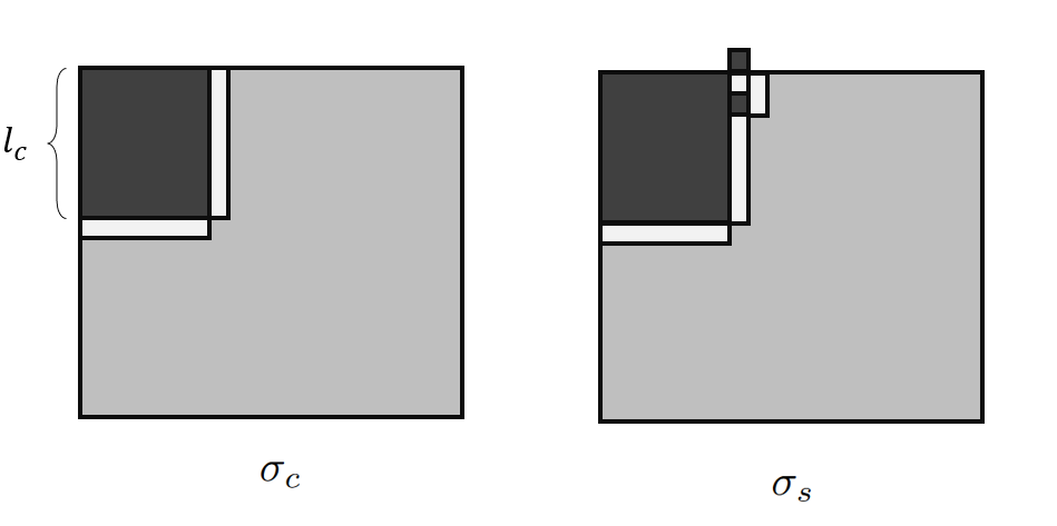
Figure 2: In the picture, white, dark gray and light gray represent the zero, plus and minus regions respectively. On the left, the configuration $\sigma_{c}$. On the right, the configuration $\sigma_{s}$ that contains two more pluses and two less minuses than $\sigma_{c}$. We note that the cluster of pluses can be attached in one of the four corners of $\Lambda$ and the protuberance can be attached along one of the two sides of the cluster of pluses.

The first result is an estimate of the stability level of all the configurations of $\mathcal{X}$ different from $\{{\boldsymbol{-1}},{\boldsymbol{+1}}\}$. This result suggests that ${\boldsymbol{-1}}$ is the unique metastable state in the region of the parameter plane under consideration.

Theorem 2.1.

Let $\eta\in\mathcal{X}$ be a configuration such that $\eta\not\in\{{\boldsymbol{-1}},{\boldsymbol{+1}}\}$, then

$$V_{\eta}\leq 6J-2(\lambda+h)+\frac{4J^{2}}{\lambda+h}=:V^{*}.$$ (2.22)

An immediate consequence of Theorem 2.1 is the recurrence of the system to the set $\{{\boldsymbol{-1}},{\boldsymbol{+1}}\}$. Indeed, by applying [31, Theorem 3.1] we have that for any $\epsilon>0$ the function

$$\beta\to\sup_{\sigma\in\mathcal{X}}\mathbb{P}_{\sigma}(\tau_{\{{\boldsymbol{-1}},{\boldsymbol{+1}}\}}>e^{\beta(V^{*}+\epsilon)})$$ (2.23)

is super–exponentially small for $\beta\to\infty$, where $\tau_{\{{\boldsymbol{-1}},{\boldsymbol{+1}}\}}$ is the first hitting time to $\{{\boldsymbol{-1}},{\boldsymbol{+1}}\}$ of the chain started at $\sigma$.

The equation (2.23) implies that the system reaches with high probability either the state ${\boldsymbol{-1}}$ (which is a local minimizer of the Hamiltonian) or the ground state in a time shorter than $e^{\beta(V^{*}+\epsilon)}$, uniformly in the starting configuration $\sigma$ for any $\epsilon>0$. In other words we can say that the dynamics speeded up by a time factor of order $e^{\beta V^{*}}$ reaches with high probability $\{{\boldsymbol{-1}},{\boldsymbol{+1}}\}$.

Theorem 2.2 (Stability level of ${\boldsymbol{-1}}$).

The stability level $V_{\boldsymbol{-1}}$ of ${\boldsymbol{-1}}$ is such that

$$H(\sigma_{c})+\Delta^{p}-H({\boldsymbol{-1}})\leq V_{\boldsymbol{-1}}\leq H(\sigma_{s})-H({\boldsymbol{-1}}).$$

We remark that the upper bound of $V_{{\boldsymbol{-1}}}$ can be estimated as follows:

$$H(\sigma_{s})-H({\boldsymbol{-1}})=2J(2l_{c}+1)+\lambda(2l_{c}-1)-h(2l_{c}^{2}+3)<\frac{2J^{2}}{h}+\frac{2J\lambda}{h}+4J+\frac{\lambda^{2}}{2h}-\frac{7}{2}h-\lambda.$$ (2.24)

Moreover, by using the explicit expression of the energy of the two configurations $\sigma_{s}$ and $\sigma_{c}$, see the equation (2.20) below, the difference between the upper and the lower bound is

$$[H(\sigma_{s})-H({\boldsymbol{-1}})]-[H(\sigma_{c})+\Delta^{p}-H({\boldsymbol{-1}})]=2J+\lambda-h.$$ (2.25)

Finally, we are now able to identify the metastable states of the system. Indeed, since the lower bound in Theorem 2.2 is strictly greater than $V^{*}$ and since all the other configurations have stability level smaller than $V^{*}$, as stated in Theorem 2.1, we have that ${\boldsymbol{-1}}$ is the configuration with maximal stability level.

Theorem 2.3 (Identification of the metastable state).

The unique metastable state is ${\boldsymbol{-1}}$.

Finally, we recall that the knowledge of the stability level of the metastable state allows to give the the asymptotic behavior as $\beta\to\infty$ of the transition time of the system started at the metastable state.

Theorem 2.4 (Asymptotic behavior of the transition time).

For any $\epsilon>0$, we have

$$\lim_{\beta\to\infty}\mathbb{P}_{{\boldsymbol{-1}}}(e^{\beta(H(\sigma_{c})+\Delta^{p}-H({\boldsymbol{-1}})-\epsilon)}<\tau_{{\boldsymbol{+1}}}<e^{\beta(H(\sigma_{s})-H({\boldsymbol{-1}})+\epsilon)})=1,$$ (2.26)

where $\tau_{\boldsymbol{+1}}$ is the first hitting time to ${\boldsymbol{+1}}$ of the chain started at ${\boldsymbol{-1}}$.

3 Proof of main results

In this section we collect the proofs of all the results stated in Section 2.

3.1 Proof of Lemma 2.1

Let $\sigma$ and $\eta$ be two communicating configurations. If $\sigma=\eta$ the statement is trivial. We consider then the case $\sigma\neq\eta$. If there exists $(x\to y)\in E$ such that $\eta=\sigma^{(x,y)}$, then the statement follows by standard Metropolis computations. On the other hand, suppose that $\eta$ and $\sigma$ differ for the value of the spin in a single site $x\in\partial^{-}\Lambda$. Several cases have to be considered:

• $\sigma(x)=+1$ and $\eta(x)=0$, we have

  $$\mu_{\beta}(\sigma)p_{\beta}(\sigma,\eta)=\frac{e^{-\beta H(\sigma)}}{Z_{\beta}}\frac{1}{2|E^{+}|}$$ (3.27)

  since the case ii) in the definition of the dynamics must be considered, and

  $$\mu_{\beta}(\eta)p_{\beta}(\eta,\sigma)=\frac{e^{-\beta H(\eta)}}{Z_{\beta}}\frac{1}{2|E^{+}|}e^{-\beta\Delta^{p}}$$ (3.28)

  since the case iii) in the definition of the dynamics must be considered. By (2.3), we obtain $H(\sigma)=H(\eta)+\Delta^{p}$ and we get that (3.27) and (3.28) are equal.

• $\sigma(x)=-1$ and $\eta(x)=0$, the proof is similar to that of case a).

• $\sigma(x)=0$ and $\eta(x)=+1$, same as case a).

• $\sigma(x)=0$ and $\eta(x)=-1$, same as case b).

We note that if $\sigma(x)=\pm 1$ and $\eta(x)=\mp 1$ with $x\in\partial^{-}\Lambda$, then $\sigma$ and $\eta$ are not communicating configurations.

3.2 Proof of Lemma 2.1

The fact that ${\boldsymbol{+1}}$ is the ground state of the Hamiltonian is achieved as in the proof of [15, Lemma 2.2] and using that $\Delta^{p},\Delta^{m}>0$.

3.3 Proof of Lemma 2.2

We observe that when a particle moves in $\Lambda$, the energy of the system increases. In particular, the energy cost to get a plus (resp. a minus) in $\Lambda$ is $\Delta^{p}$ (resp. $\Delta^{m}$). This implies that the state ${\boldsymbol{0}}$ is a local minumun. Moreover, also the state ${\boldsymbol{-1}}$ is a local minimum of the Hamiltonian, since the other possible moves have a positive energy cost, indeed a minus may move from $\Lambda_{0}$ in $\partial^{+}\Lambda_{0}$ with an energy cost greater than (exit from the boundary) or equal to (exit from the corner) $4J$.

3.4 Auxiliary lemmas

In this section we collect some auxiliary lemmas that wil be used in the proof of the following theorems. The proofs of these lemmas are in Section 4.

First of all, given a configuration $\eta\in\mathcal{X}$, we consider the set $\mathcal{C}(\eta)\subseteq\mathbb{R}^{2}$ defined as the union of the closed unitary squares centered at sites of $\Lambda_{0}$ with the boundary parallel to the axes of $\mathbb{Z}^{2}$ and such that the spin in $\eta$ associated with the site is plus. The maximal connected components $C_{1},\dots,C_{m}$, with $m\in\mathbb{N}$, of $\mathcal{C}(\eta)$ are called clusters of pluses. We define in the same way the clusters of minuses and the clusters of zeros. The boundary of each cluster is made of straight lines and corners on the dual lattice, that can be convex corners or concave corners following the usual $\mathbb{R}^{2}$ definitions. Moreover, the portion of the boundary of the cluster delimited by two subsequent convex corners is called a convex side of the cluster, otherwise, if at least one of the two corners is concave, it is called a concave side. We observe that each cluster has at least one convex side, since $\Lambda_{0}$ is finite (and, recall, it is not a torus).

Moreover, given a configuration $\sigma\in\mathcal{X}$, a zero-carpet of $\sigma$ is a connected set $X\subset\Lambda$ such that $\sigma(x)=0$ for each $x\in X$. In a similar way we define the s-carpet of $\sigma$ with $s\in\{-1,+1\}$.

The following lemma is a key result of this paper. Indeed, here we show that if a particle, indifferently a plus or a minus, is transported along a zero carpet, then it possible to reduce the computation of the difference of energy between any two configurations visitec along the path to the examination of nine possible cases. Moreover, the height of this path in the configuration space equals the height computed along the corresponding path on the graph by summing the weights of each transition. We use this property to prove a bound for the height of the path in the configuration space which does not depend on its length.

Lemma 3.4 (Weighted graph for the energy cost in a carpet).

Let $s\in\{-1,0,+1\}$. Consider a configuration $\sigma\in\mathcal{X}$ such that there exists a $s$-carpet $X$ of $\sigma$ and two nearest neighboring sites $x\in\Lambda\setminus X$ and $x^{\prime}\in X$ such that $\sigma(x)=r\neq s$. Assume, also, that there exists $y\neq x^{\prime}$ a nearest neighbor of $x$ such that $\sigma(y)=s$. Let $X^{\prime}$ be the subset of $X$ obtained by collecting $x^{\prime}$ together with all the sites of $X$ having at least two neighboring sites in $X$. Then the following holds:

1. for any $v\in X^{\prime}\cup\{x\}$, let $\sigma^{v}=\sigma^{(x,v)}$ and recall that $\sigma^{(x,x)}$ is equal to $\sigma$. Then, for any pair of neighboring sites $v,w\in X^{\prime}\cup\{x\}$

   $$H(\sigma^{v})-H(\sigma^{w})\in\begin{cases}\{-8J,-6J,-4J,-2J,0,2J,4J,6J,8J\}\qquad&\text{ if }s=0,\\ \{-8J,-6J,-4J,-2J,0,2J,4J,6J,8J\}\qquad&\text{ if }s\neq 0\text{ and }r=0,\\ \{-16J,-12J,-8J,-4,0,4J,8J,12J,16J\}\qquad&\text{ if }s\neq 0\text{ and }r=-s.\end{cases}$$

   can be computed as specified in the Figure 3.

2. For any $v\in X^{\prime}$

   $$\Phi(\sigma,\sigma^{v})-H(\sigma)\leq\begin{cases}8J\qquad&\text{ if }s=0,\\ 8J\qquad&\text{ if }s\neq 0\text{ and }r=0,\\ 16J\qquad&\text{ if }s\neq 0\text{ and }r=-s.\end{cases}$$

     

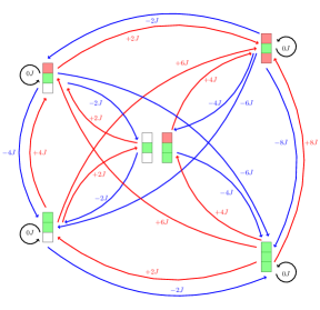
Figure 3: In each vertex of the graph the three squares represent three sites such that the one at the center is the site $x$ and it is nereast neighbor of the other two. The local configuration is reported with the colors red, green and white representing, respectively, the spin values $s\neq 0$, $-s$, and 0. The other two sites neighboring the middle square and not reported in the picture are occupied by a zero spin in the left panel, and by a $s$ spin in the center and right panel. The vertex at the center of the graph corresponds to any of the two reported configurations. Any transition from $\sigma^{v}$ to $\sigma^{w}$ for $v,w\in X^{\prime}\cup\{x\}$ is realized via the swap of the particle between two sites with local configuration represented by one of the vertices of the graph. For each possible swap the energy difference is reported in the picture.

In the next lemma, we show that if a particle is transported inside or outside $\Lambda_{0}$ through a carpet, than Lemma 3.4 can be used to bound the height of the path by $18J$.

Lemma 3.5 (Transport through a zero-carpet).

Consider a configuration $\sigma\in\mathcal{X}$ such that there exists a zero-carpet $X$ of $\sigma$ such that $X\cap\partial^{-}\Lambda_{0}\neq\emptyset$.

• Given $x\in X$, let $\eta:=\sigma^{(x;s)}$ with $s\in\{-1,+1\}$, then

  $$\Phi(\sigma,\eta)-H(\sigma)\leq 18J\qquad\text{and}\qquad H(\eta)=H(\sigma)+\Delta_{s}-2D_{x}(\eta)J,$$ (3.29)

  where $D_{x}(\eta)$ is defined in 2.11.

• Given $x\in\Lambda_{0}$ a nearest neighbor of $X$ such that $\sigma(x)=s\neq 0$. Let $\eta:=\sigma^{(x;0)}$, then

  $$\Phi(\sigma,\eta)-H(\sigma)\leq 14J\qquad\text{and}\qquad H(\eta)=H(\sigma)+2D_{x}(\sigma)J-\Delta_{s}.$$ (3.30)

In words, in $(i)$ we state that to transport a plus or a minus through a zero-carpet from outside to a site $x$ with spin zero, has an energy cost smaller than or equal to $18J$ and the energy of the final configuration depends on the local configuration around $x$. While, in $(ii)$, we state that a plus or a minus in the site $x$ follows a zero-carpet and then it leaves $\Lambda$ with an energy cost smaller than or equal to $10J$; also in this case the energy of the final configuration depends on the local configuration around $x$.

Lemma 3.6 (Transport through a $s$-carpet).

Consider a configuration $\sigma\in\mathcal{X}$ such that there exists a $s$-carpet $X$ of $\sigma$ such that $X\cap\partial^{-}\Lambda_{0}\neq\emptyset$ and $y\in\Lambda$ a nearest neighbor of $X$.

• If $\sigma(y)\neq 0$, then let $\eta:=\sigma^{(y;0)}$ and we have

  $$\Phi(\sigma,\eta)-H(\sigma)\leq 54J\qquad\text{and}\qquad H(\eta)=H(\sigma)+2D_{y}(\sigma)J-\Delta_{s},$$ (3.31)

  where $D_{y}(\sigma)$ is defined in 2.11.

• If $\sigma(y)=0$, then let $\eta:=\sigma^{(y;s)}$ and we have

  $$\Phi(\sigma,\eta)-H(\sigma)\leq 35J\qquad\text{and}\qquad H(\eta)=H(\sigma)+\Delta_{s}-2D_{y}(\eta)J.$$ (3.32)

In words, in $(i)$ a particle with spin $-s$ follows a $s$-carpet from its position $y$ to $\partial^{+}\Lambda_{0}$ and then it is replaced by a zero. This zero runs through the $s$-carpet until it reaches the site $y$. This path has an energy cost smaller than or equal to $38J$ and the energy of the final configuration depends only on the local configuration around $y$. While, $(ii)$ considers the motion of the zero initially in $x$ along the $s$-carpet, until it reaches $\partial^{-}\Lambda_{0}$. Hence, this zero is exchanged with a particle with spin $s$ created in $\partial^{+}\Lambda_{0}$. The energy cost of this path is smaller than or equal to $54J$ and the energy of the final configuration depends only on the local configuration around $y$.

We will now state some lemmas in which we use the notion of carpet to estimate the stability level of some specified configurations. Before stating the lemmas we need a new definition.

Lemma 3.7.

Let $\sigma$ be a configuration that contains a bond of type $(+,-)$. Assume that there exists a zero-carpet of $\sigma$ at distance one from the bond and intersecting $\partial^{-}\Lambda_{0}$ or the bond is at distance one from $\partial^{+}\Lambda_{0}$, then $V_{\sigma}\leq 14J$.

Lemma 3.8.

Let $\sigma$ be a configuration that contains a bond of type $(+,-)$ and let $s\in\{-1,+1\}$. If there exists a $s$-carpet of $\sigma$ at distance one from $\partial^{+}\Lambda_{0}$ and from the site of the bond with spin $-s$, then $V_{\sigma}\leq 54J$.

Lemma 3.9.

Let $x\in\Lambda$ and let $x_{i}$ be the nearest neighbours of $x$, with $i=1,\dots,4$. Let $\sigma$ be a configuration such that $\sigma(x)=0$, $\sigma(x_{1})=\sigma(x_{2})=+1$, $\sigma(x_{3})=0$, and $\sigma(x_{4})\neq-1$ or $\sigma(x_{4})=-1$ with at most two nearest neighbors equal to $-1$. If there exists a zero-carpet of $\sigma$ at distance one from $x$ and intersecting $\partial^{+}\Lambda_{0}$, then $V_{\sigma}<18J$.

Lemma 3.10.

Let $\sigma$ be a configuration that contains a cluster of pluses (resp. minuses) with at least a convex side with length $l\leq\lfloor\frac{2J}{\lambda+h}\rfloor$ (resp. $l\leq\lfloor\frac{2J}{\lambda-h}\rfloor$). Assume that there exists a zero-carpet of $\sigma$ at distance one from one of the two corner sites of the convex side of the cluster and intersecting $\partial^{+}\Lambda_{0}$. Then $V_{\sigma}<16J$.

Lemma 3.11.

Let $\sigma$ be a configuration that contains a cluster of pluses (resp. minuses) with at least a convex side with length $l\geq\lfloor\frac{2J}{\lambda+h}\rfloor+1$ (resp. $l\geq\lfloor\frac{2J}{\lambda-h}\rfloor+1$) at distance strictly greater than two from a minus spin (resp. plus spin). Assume that there exists a zero-carpet of $\sigma$ at distance one from one of the two corner sites of the convex side of the cluster and intersecting $\partial^{+}\Lambda_{0}$. Then $V_{\sigma}<22J$.

We note that in the previous two lemmas, if the cluster is at distance one from $\partial^{+}\Lambda_{0}$, then there exists a zero carpet, at distance one the two corner sites of the convex side, composed by only sites in $\partial^{+}\Lambda_{0}$.

Lemma 3.12.

Let $\sigma$ be a configuration that contains a flag-shaped structure namely a structure made of a strip of pluses, a strip of zeros and a strip of minuses with equal lengths as in the left or right panel of Figure 4. Assume that there exists a minus-carpet of $\sigma$ at distance one from the strip of zeros, then $V_{\sigma}<58J$.

Figure 4: Representation of the flag-shaped structure present in the configuration considered in Lemma 3.12. We note that the strips can be vertical or horizontal.

Lemma 3.13.

We have that $V_{\boldsymbol{0}}\leq 6J-2(\lambda+h)+4J^{2}/(\lambda+h)$.

3.5 Proof of Theorem 2.1

In order to prove Theorem 2.1 we start showing that the stability level of each configuration $\eta\not\in\{{\boldsymbol{-1}},{\boldsymbol{+1}}\}$ is smaller than or equal to $V^{*}$. First of all, we note that if $\eta$ contains some plus or minus spin in $\partial^{+}\Lambda_{0}$, then $V_{\eta}=0$ indeed the particle with plus (resp. minus) spin leaves $\Lambda$ and the energy decreases by $\Delta^{p}$ (resp. $\Delta^{m})$. Thus, from now on we assume $\eta_{\partial^{+}\Lambda_{0}}=0_{\partial^{+}\Lambda_{0}}$. To prove that $V_{\eta}<V^{*}$, we partition the set of all configurations according to the value of the spin in the upper-left corner, that we denote by $x_{0}=(1,L)$, and we use the auxiliary lemmas 3.7-3.13. In the following the columns are ordered from left to right and the row from top to bottom.

Case $\eta(x_{0})=0$.

Let $R$ be the maximal rectangle with the upper-left corner in the $x_{0}$ and such that $\eta_{R}=0_{R}$. We note that if $R\equiv\Lambda_{0}$, i.e. $\eta\equiv{\boldsymbol{0}}$, then we conclude by using Lemma 3.13. Thus, assume $R\not\equiv\Lambda_{0}$ and let $l_{v},l_{h}$ be, respectovely, the vertical and horizontal side lengths of $R$.

If $l_{v},l_{h}\geq\lfloor\frac{2J}{\lambda+h}\rfloor+1$, then we reduce the energy of $\eta$ with an energy cost strictly smaller than $V^{*}$ by using the same path described in the proof of Lemma 3.13.

Thus, assume that at least one of the two lengths (for instance $l_{h}$) is smaller than or equal to $\lfloor\frac{2J}{\lambda+h}\rfloor+1$. Since, $R$ is maximal it follows that there exists $x_{2}\in\{L-l_{v}+1,\dots,L\}$ such that, denoted $x=(l_{h}+1,x_{2})$, we have $\eta(x)\neq 0$ and $\eta(x+je_{2})=0$ for $j=1,\dots,L-x_{2}$. We let, also, $y=x-(m-1)e_{2}$, with $m\geq 1$ integer, be such that $\eta(x-je_{2})=\eta(x)$ for every $0\leq j\leq m-1$ and $\eta(y-e_{2})\neq\eta(y)$. We distinguish two cases, see Figure 5:

Figure 5: Representation of the configurations used in items (i) and (ii) of Case $\eta(x_{0})=0$ in the proof of the Theorem 2.1, respectively, on the left and on the right.

• Case $x_{2}-m\geq L-l_{v}+1$: if $m\leq\lfloor\frac{2J}{\lambda\pm h}\rfloor$, we consider the configuration in which the spins in $x-je_{2}$, with $j=0,\dots,m-1$, are changed to $0$, and note that, by Lemma 3.10, such a configuration has energy smaller that the initial one and the communication height is smaller than $10J$ which, in turn, is smaller than $V^{*}$. On the other hand, if $m\geq\lfloor\frac{2J}{\lambda\pm h}\rfloor+1$, we consider the configuration in which the zeroes at sites $(l_{h},x_{2}-j)$ with $j=0,\dots,m-1$ are changed to $\eta(x)$ and the theorem follows from Lemma 3.11.

• Case $x_{2}-m\leq L-l_{v}$, and assume that there exists a site $z=(l_{h},z_{2})$ for some $x_{2}-(m-1)-1\leq z_{2}\leq L-l_{v}$ such that $\eta(z)\neq 0$ and $\eta(l_{h},a)=0$ for $a\geq z_{2}+1$, see Figure 6. We distinguish two cases:

  • $\eta(z)=-\eta(x)$. We conclude by applying Lemma 3.7.

  • $\eta(z)=\eta(x)$. We consider the site $w=z+e_{2}$ and assume that $\eta(w-e_{1})\neq-\eta(x)$. If necessary, we add a particle with spin $\eta(x)$ in $\partial^{+}\Lambda_{0}$, by paying either $\Delta^{p}$ or $\Delta^{m}$. Then we transport the particle trough the zero-carpet to $w$, by paying $8J$, see Lemma 3.4. By direct inspection we also get that the difference of energy between the final and the initial configurations is smaller than or equal to $-(\lambda\pm h)$. On the other hand, in the case $\eta(w-e_{1})=-\eta(x)$, we conclude by applying Lemma 3.7.

  

  Figure 6: Representation of the configurations in items (ii.a) and (ii.b) of Case $\eta(x_{0})=0$ in the proof of the Theorem 2.1, respectively, on the left and on the right.

• Case $x_{2}-m\leq L-l_{v}$, and assume that all the spins associated with the sites $(l_{h},a)$ with $a\geq x_{2}-(m-1)-1$ are zero.

  In the case $m\leq\lfloor\frac{2J}{\lambda\pm h}\rfloor$, we proceed exactly as in case (i) above.

  

  

  Figure 7: Left: Representation of the configuration used in case (iii) of Case $\eta(x_{0})=0$ in the proof of the Theorem 2.1. Right: An example of configuration $\eta$ of point (ii) in Case $\eta(x_{0})=+1$.

  On the other hand, in the case $m\geq\lfloor\frac{2J}{\lambda\pm h}\rfloor+1$, we have to look at the spins in the column $l_{h}-1$. If all the sites $(l_{h}-1,j)$ with $j\geq x_{2}-(m-1)$ have spin zero, then we get the proof again as in case (i) above. Otherwise, namely, if at least one of the spins associated with the sites $(l_{h}-1,j)$ with $j\geq x_{2}-(m-1)$ is not zero, then we have to look at the sites along the row $L-l_{v}$. Since $R$ is maximal, there exists a site $k=(k_{1},L-l_{v})$ such that $\eta(k)\neq 0$ and $\eta(j,L-l_{v})=0$ for $j=1,\dots,k_{1}-1$. Let $q=k+ne_{1}$, with $n\geq 0$ integer, be such that $\eta(k+je_{1})=\eta(k)$ for $0\leq j\leq n$ and $\eta(k)\neq\eta(q+e_{1})$, see the left panel in Figure 7. If $n\leq\lfloor\frac{2J}{\lambda\pm h}\rfloor$ we conclude by using Lemma 3.10 and if $n\geq\lfloor\frac{2J}{\lambda\pm h}\rfloor+1$ we conclude by using Lemma 3.11.

Case $\eta(x_{0})=+1$.

Let $R$ be the maximal rectangle with the upper-left corner in the $x_{0}$ and such that $\eta_{R}=+1_{R}$. We note that $R\not\equiv\Lambda_{0}$, otherwise $\eta\equiv{\boldsymbol{+1}}$.

Thus, let $l_{v},l_{h}$ be, respectively, the vertical and horizontal side lengths of $R$. Since $R$ is maximal, it follows that there exists a spin different from plus at distance one from $R$.

In case it is a minus, we conclude by applying Lemma 3.7, if the associated site is in $\partial^{-}\Lambda_{0}$, otherwise we conclude by applying Lemma 3.8.

Now, we consider the case in which all the spins at distance one from $R$ are pluses and zeros. Without loss of generality, we can assume that there exists a site on the vertical part of the external boundary of $R$ with associates spin equal to zero. Thus, we let $x_{2}\in\{L-l_{v}+1,\dots,L\}$ be such that, denoted $x=(l_{h}+1,x_{2})$, we have $\eta(x)=0$ and $\eta(x+je_{2})=+1$ for $j=1,\dots,L-x_{2}$.

We note that if $x\not\in\partial^{-}\Lambda_{0}$, see the left panel in Figure 8, then we apply Lemma 3.6 or Lemma 3.9 and we conclude.

Figure 8: Representation of the configuration used in the case $\eta(x_{0})=+1$ in the proof of Theorem 2.1.

We are thus left with the case $x\in\partial^{-}\Lambda_{0}$, i.e., $x_{2}=L$. In such a case we let $y=x-(m-1)e_{2}$, with $m\geq 1$ integer, be such that $\eta(x-je_{2})=\eta(x)$ for every $0\leq j\leq m-1$ and either $y-e_{2}\in\partial^{+}\Lambda_{0}$ or $\eta(y-e_{2})\neq\eta(y)$, see the center and right panel in Figure 8. We distinguish two cases:

• Case $m\leq l_{v}-1$: we can conclude since $\eta$ satisfies the assumption of Lemma 3.5-(i), indeed, $\eta(y)=0$, $\eta(y-e_{1})=+1$ (inside $R$), $\eta(y-e_{2})=+1$ (otherwise there would be a minus in $\partial^{+}R$), and if $\eta(y+e_{1})$ were minus, then it would not have three neighboring minuses because in such a case there would be a direct $(+,-)$ interface in the sites $y-e_{2}$ and $y+e_{1}-e_{2}$. See the center panel in Figure 8.

• Case $m\geq l_{v}$. If $l_{v}\leq\lfloor\frac{2J}{\lambda+h}\rfloor$, then we reduce the energy of $\eta$ with an energy cost strictly smaller than $V^{*}$ by using Lemma 3.10. If $l_{v}\geq\lfloor\frac{2J+\lambda-h}{2h}\rfloor+1$, we conclude by using Lemma 3.12.

  We are thus left with the case $\lfloor\frac{2J+\lambda-h}{2h}\rfloor\geq l_{v}\geq\lfloor\frac{2J}{\lambda+h}\rfloor+1$ with which we deal by looking at the value of the spins at distance $\sqrt{2}$ and $2$ from the side of $R$ with length $l_{h}$.

  If one of these spins is plus we apply Lemma 3.5-(i) and if they are all zeros we conclude by applying Lemma 3.11. We are left with the case in which these spins are either zero or minus and at least one of them is minus, see Figure 9. We distinguish two cases:

  

  Figure 9: Representation of the configuration used in the case $\eta(x_{0})=+1$ in the proof of Theorem 2.1.

  • all these spins are zeros excepted the one at distance $\sqrt{2}$ which has spin minus, see the left panel in Figure 9.

    We note that if this minus has three minus nearest neighbours, then one of them is at distance one from $R$ and so we conclude by applying Lemma 3.8.

    Thus, we assume that the minus has at most two nearest neighbors with minus spin. Let $\eta^{\prime}$ be the configuration obtained from $\eta$ by replacing the minus at distance $\sqrt{2}$ with a zero, and let $\eta^{\prime\prime}$ be the configuration obtained from $\eta^{\prime}$ by replacing with plus the zeros at distance one from the side of the rectangle with length $l_{v}$, see Figure 10. We consider the following path which starts from $\eta$ and ends in $\eta^{\prime\prime}$ crossing $\eta^{\prime}$: the minus is transported along the (vertical in the figure) column adjacent to $R$ and, after it reaches the external boundary $\partial^{+}\Lambda_{0}$, it is removed. Then, one after the other, $l_{v}$ pluses are created in $\partial^{+}\Lambda_{0}$ and transported along the same column to their final location as reported in panel of Figure 10. We have that $H(\eta^{\prime})=H(\eta)+(\lambda-h)$ and $H(\eta^{\prime\prime})=H(\eta^{\prime})+2J-l_{v}(\lambda+h)$. Then, we obtain $H(\eta^{\prime\prime})\leq H(\eta)+(\lambda-h)+2J-\Big{(}\frac{2J}{\lambda+h}+1\Big{)}(\lambda+h)<H(\eta)$. Moreover, by direct inspection, we have that the height along the considered path is smaller than or equal to $6J$.

    

    Figure 10: On the left the initial configuration $\eta$ of point (i) in Case $\eta(x_{0})=+1$. On the right the final configuration $\eta^{\prime\prime}$.

  • There is at least a minus spin at distance $2$ from the side of $R$ with length $l_{v}$.

    We denote by $k=(l_{h}+2,k_{2})$ the site with minus spin and at minimal distance from $\partial^{+}\Lambda_{0}$, see the right panel in Figure 9.

    If $L-k_{2}\geq\lfloor\frac{2J}{\lambda+h}\rfloor+1$, then we replace with pluses the first (from the top) $L-k_{2}$ zeroes in the vertical column adjacent to $R$, by applying Lemma 3.11 we prove the theorem.

    On the contrary, suppose, now, that $L-k_{2}\leq\lfloor\frac{2J}{\lambda+h}\rfloor$.

    We consider the rectangular region $D$ of $\Lambda_{0}$ with the upper-left corner in $(l_{h}+2,L)$ and the down-right corner in $k+ne_{1}$ where $n\in\{l_{h}+2,...,L\}$ is such that $\eta(k+je_{1})=\eta(k)$ for every $0\leq j\leq n$ and $\eta(k+ne_{1})\neq\eta(k)$, see the right panel in Figure 7. Notice that the horizontal strip from $k$ to $k+ne_{1}$ contained in $D$ is a strip of minuses by construction. Let $p\in D$ be the site with the minus spin according to the lexicographic order. We note that $p$ can be $k$ by construction. We consider the rectangular region $D_{1}\subset D$ with the upper-left corner in $(l_{h}+1,L)$ and the down-left corner in $(p_{1}-1,k_{1}+1)$. We observe that by construction in $D_{1}$ there are not minus spins, see the right panel in Figure 7. If there is a plus spin at distance one from the strip of minuses containing $k$ in the rectangular region $D_{1}$, then we conclude by applying Lemma 3.7. Thus, we are left with the case in which there are only zeros at distance one from this strip. Assume, first, that in $D_{1}$ there is a cluster of pluses, then it necessarily has a convex side length smaller than $\lfloor\frac{2J}{\lambda+h}\rfloor$. Then, we conclude by applying Lemma 3.11. Thus, in $D_{1}$ there are only zero spins. and we consider the rectangular region $D_{2}$ with the upper-left corner in $(p_{1},L)$ and the down left corner in $p+ae_{1}$ where $a\in\{l_{h}+2,...,L\}$ is such that $\eta(p+ae_{1})=\eta(k)$ for every $0\leq j\leq a$ and $\eta(p+ae_{1})\neq\eta(p)$, see the right panel in Figure 7.

    Assume $D_{2}\neq\emptyset$. Notice that the horizontal strip from $p$ to $p+ae_{1}$ is a strip of minuses by construction. If there is a plus spin at distance one from this strip, then we conclude by applying Lemma 3.7. We observe that by construction in $D_{2}$ there are not minus spins and we assume, first, that in $D_{2}$ there is a cluster of pluses. This cluster necessarily has a convex side length smaller than $\lfloor\frac{2J}{\lambda+h}\rfloor$ by construction, thus we conclude by applying Lemma 3.11. Thus, in $D_{2}$ there are only zeros and we consider the length $a$ of the strip of minuses containing $p$.

    If $a\leq\lfloor\frac{2J}{\lambda-h}\rfloor$ we conclude by applying Lemma 3.10.

    Otherwise if $a\geq\lfloor\frac{2J}{\lambda-h}\rfloor+1$, we distinguish two cases:

    • The site at distance $\sqrt{2}$ from the strip of minus has spin different from plus. In this case, we apply Lemma 3.11 and we prove the Theorem.

    • The site at distance $\sqrt{2}$ from the strip of minus has plus spin. We denote by $z$ this site and we note that if $\eta(z-e_{2})=+1$, then there is a direct $(+,-)$ interface in the sites $z-e_{2}$ and $z-e_{1}-e_{2}$. Thus, we conclude by applying Lemma 3.5-(ii) to the site $z-e_{1}-e_{2}$. Otherwise if $\eta(z-e_{2})=0$, then we can conclude by applying Lemma 3.10 to the cluster of pluses containing $z$.

    If $D_{2}=\emptyset$, i.e. $p\equiv k$, then we proceed as above by applying the same procedure to $D_{1}$.

Case $\eta(x_{0})=-1$.

Let $R$ be the maximal rectangle with the upper-left corner in the $x_{0}$ and such that $\eta_{R}=-1_{R}$. We note that $R\not\equiv\Lambda_{0}$, otherwise $\eta\equiv{\boldsymbol{-1}}$.

Thus, let $l_{v},l_{h}$ be, respectively, the vertical and horizontal side lengths of $R$. Since $R$ is maximal, it follows that there exists a spin different from minus at distance one from $R$.

In case it is a plus, we conclude by applying Lemma 3.7 if the associated site is in $\partial^{-}\Lambda_{0}$, otherwise we conclude by applying Lemma 3.8.

Then, we consider the case in which all the spins at distance one from $R$ are minuses and zeros. Without loss of generality, we can assume that there exists a site on the vertical part of the external boundary of $R$ with an associated spin equal to zero. Thus, we let $x_{2}\in\{L-l_{v}+1,\dots,L\}$ be such that, denoted $x=(l_{h}+1,x_{2})$, we have $\eta(x)=0$ and $\eta(x+je_{2})=-1$ for $j=1,\dots,L-x_{2}$.

We distinguish two cases:

• Case $x_{2}\not=L$. We consider the cluster of minuses $C$ containing $R$. If $\partial^{+}C$ contains a plus spin, then we conclude by using Lemma 3.8. Thus, suppose that $\partial^{+}C$ contains only zero spins. Either $\eta\equiv{\boldsymbol{-1}}$ or we denote by $p=(p_{1},p_{2})$ with $p_{1},p_{2}\in\{1,...,L\}$ the first site such that $\eta(p)=0$ in lexicographic order. If $p_{2}=L$, then we proceed as in case (ii) below assuming $p\equiv x$. Otherwise if $p_{2}=L-j$ with $L-1\geq j>0$, then all spins with vertical coordinate $L,L-1,...,L-(j-1)$ are minus and we look at sites $p+e_{1}$ and $p-e_{2}$. If $\eta(p+e_{1})=-1$ or $\eta(p-e_{2})=-1$, then we conclude by applying Lemma 3.6. If $\eta(p+e_{1})=\eta(p-e_{2})=0$, then we prove the statement by using Lemma 3.6. We are thus left with the case $\eta(p+e_{1})=0$ and $\eta(p-e_{2})=+1$, indeed we recall that $p+e_{1}\in\partial^{+}\Lambda_{0}$ or $p+e_{1}\in\partial^{+}C$, so $\eta(p+e_{1})\neq+1$. We consider the strip of pluses containing $p-e_{2}$ and we observe that if there exists a site at distance one from this strip with vertical coordinate $p_{2}+1$ with spin different from zero, then we can apply Lemma 3.8 and we conclude. Thus, all the sites at distance one from this strip with vertical coordinate $p_{2}+1$ are zero and we prove the statement by using Lemma 3.12.

• Case $x_{2}=L$. In such a case we let $y=x-(m-1)e_{2}$, with $m\geq 1$ integer, be such that $\eta(x-je_{2})=\eta(x)$ for every $0\leq j\leq m-1$ and either $y-e_{2}\in\partial^{+}\Lambda_{0}$ or $\eta(y-e_{2})\neq\eta(y)$. We distinguish two cases:

  • Case $m\leq l_{v}-1$. Assume first $\eta(y+e_{1})\neq+1$, then we can conclude since $\eta$ satisfies the assumption of Lemma 3.5-(i), indeed, $\eta(y)=0$, $\eta(y-e_{1})=-1$ (inside $R$), $\eta(y-e_{2})=-1$ (otherwise there would be a plus in $\partial^{+}R$).

    Now, suppose that $\eta(y+e_{1})=+1$ and let $w=y+e_{1}+ne_{2}$ with $n$ be such that $\eta(y+e_{1}+je_{2})=\eta(y+e_{1})$ for every $0\leq j\leq m-1$ and either $w+e_{2}\in\partial^{+}\Lambda_{0}$ or $\eta(w+e_{2})\neq\eta(y+e_{1})$.

    If $L-(y_{2}+\tilde{j})-1\geq\lfloor\frac{2J}{\lambda-h}\rfloor+1$, then we apply Lemma 3.11 to the part of the side of $R$ with length $L-(y_{2}+\tilde{j})-1$ and we prove the theorem.

    On the contrary, if $L-(y_{2}+\tilde{j})-1\leq\lfloor\frac{2J}{\lambda-h}\rfloor$, we consider the rectangle of $\Lambda_{0}$ with the upper-left corner in $(l_{h}+2,L)$ with side lengths $L-(y_{2}+\tilde{j})$ and $l_{s}$, where $l_{s}$ is the horizontal length of the strip of pluses containing $\eta(w)$. If inside of this rectangle there is a minus spin at distance one from this strip of pluses, then we conclude by applying Lemma 3.7. Thus, assume that inside the rectangle there are only zeros and pluses at distance one from this strip and assume, first, that in the rectangular region there is a cluster of minuses, then it necessarily has a convex side length smaller than $L-(y_{2}+\tilde{j})-1\leq\lfloor\frac{2J}{\lambda-h}\rfloor$. Then, we conclude by applying Lemma 3.11.

    Now, assume that in this rectangular region there is a mixture of pluses and zeros. If the cluster of pluses containing $\eta(w)$ has a concave side or there are some plus spins at distance two from it, then we conclude by applying Lemma 3.5-(i). In the other case, we consider the length $n$.

    If $l_{s}\leq\lfloor\frac{2J}{\lambda+h}\rfloor$ we conclude by applying Lemma 3.10.

    Otherwise if $l_{s}\geq\lfloor\frac{2J}{\lambda+h}\rfloor+1$, we distinguish two cases:

    • The site $z$ at distance $\sqrt{2}$ from the strip of pluses and at distance one from the rectangle $S$ has spin different from minus. In this case, we apply Lemma 3.11 and we prove the Theorem.

    • The site $z$ at distance $\sqrt{2}$ from the strip of pluses and at distance one from the rectangle $S$ has minus spin. We conclude as in case $\eta(x_{0})=+1$ (ii.a).

  • Case $m\geq l_{v}$. If $l_{v}\leq\lfloor\frac{2J}{\lambda-h}\rfloor$, then we reduce the energy of $\eta$ with an energy cost strictly smaller than $V^{*}$ by using Lemma 3.10. We are thus left with the case $l_{v}\geq\lfloor\frac{2J}{\lambda-h}\rfloor+1$ with which we deal by looking at the value of the spins at distance $\sqrt{2}$ and $2$ from the vertical side of $R$.

    Assume first that the spin at distance $\sqrt{2}$ is different from plus. If all the sites at distance 2 have zero spin, then we apply Lemma 3.11. If one of the spins at distance 2 is minus we apply Lemma 3.5-(i).

    Now, we suppose that the spin at distance $\sqrt{2}$ is plus. If there is a minus spin in a site $d=(l_{h}+2,d_{2})$ such that $d_{2}\neq L-l_{v}-1$, then we apply Lemma 3.5-(i). Otherwise, if $d_{2}=L-l_{v}-1$ then we analyze the spins at the right and the left of the site $d-e_{1}-e_{2}$, i.e. the site of the plus spin at distance $\sqrt{2}$ from the rectangle. If one of them is plus, then we apply Lemma 3.5 at the minus at site $d$ or $d-2e_{1}$. Otherwise, we apply the Lemma 3.5 at the plus in $d-e_{1}-e_{2}$,.

    We are left with the case in which spins are either zero or plus at distance 2 and $\sqrt{2}$ and at least one of them is plus. We distinguish two cases:

    • all these spins are zeros excepted the one at distance $\sqrt{2}$ which has spin plus. We denote by $q=(l_{h}+1,L-l_{v})$ the corresponding site. If $l_{v}-1\geq\lfloor\frac{2J}{\lambda-h}\rfloor+1$, then we apply Lemma 3.11 and we prove the theorem.

      On the contrary, suppose that $l_{v}-1\leq\lfloor\frac{2J}{\lambda-h}\rfloor$.

      We consider the rectangular region $D$ of $\Lambda_{0}$ with the upper-left corner in $(l_{h}+1,L)$ and the down-right corner in $q+ne_{1}$ where $n\in\{l_{h}+2,...,L\}$ is such that $\eta(q+je_{1})=\eta(q)$ for every $0\leq j\leq n$ and $\eta(q+ne_{1})\neq\eta(q)$. Notice that the horizontal strip from $q$ to $n$ contained in $D$ is a strip of pluses by construction. Let $p\in D$ be the site with the first plus spin according to the lexicographic order. We note that $p$ can be $q$ by construction. We consider the rectangular region $D_{1}\subset D$ with the upper-left corner in $(l_{h}+1,L)$ and the down-left corner in $(p_{1}-1,q_{1}+1)$. We observe that by construction in $D_{1}$ there are not plus spins. If there is a minus spin at distance one from the strip of pluses containing $q$ in the rectangular region $D_{1}$, then we conclude by applying Lemma 3.7. Thus, we are left with the case in which there are only zeros at distance one from this strip. Assume, first, that in $D_{1}$ there is a cluster of minuses, then it necessarily has a convex side length smaller than $l_{v}-1\leq\lfloor\frac{2J}{\lambda-h}\rfloor$. Then, we conclude by applying Lemma 3.11. Thus, in $D_{1}$ there are only zero spins and we consider the rectangular region $D_{2}$ with the upper-left corner in $(p_{1},L)$ and the down left corner in $p+ae_{1}$ where $a\in\{p_{1},...,L\}$ is such that $\eta(p+ae_{1})=\eta(p)$ for every $0\leq j\leq a$ and $\eta(p+ae_{1})\neq\eta(p)$. Assume $D_{2}\neq\emptyset$. Notice that the horizontal strip from $p$ to $p+ae_{1}$ is a strip of pluses by construction. If there is a minus spin at distance one from this strip, then we conclude by applying Lemma 3.7.

      We observe that by construction in $D_{2}$ there are not plus spins and we assume, first, that in $D_{2}$ there is a cluster of minuses. This cluster necessarily has a convex side length smaller than $l_{v}-1\leq\lfloor\frac{2J}{\lambda-h}\rfloor$ by construction, thus we conclude by applying Lemma 3.11.

      Thus, in $D_{2}$ there are only zeros and we consider the length $a$ of the strip of pluses containing $p$. If $a\leq\lfloor\frac{2J}{\lambda+h}\rfloor$, then we conclude by applying Lemma 3.11. If $a\geq\lfloor\frac{2J}{\lambda+h}\rfloor+1$, we distinguish two cases:

      • The site at distance $\sqrt{2}$ from the strip of pluses has spin different from minus. In this case, we apply Lemma 3.11 and we prove the Theorem.

      • The site at distance $\sqrt{2}$ from the strip of pluses has minus spin. We conclude by building two configurations $\eta^{\prime}$ and $\eta^{\prime\prime}$ and by proceeding as in case $\eta(x_{0})=+1$ (ii.a).

      If $D_{2}=\emptyset$, i.e. $p\equiv q$, then we proceed as above by applying the same procedure to $D_{1}$.

    • We denote by $k=(l_{h}+2,k_{2})$ the site with plus spin and at minimal distance from $\partial^{+}\Lambda_{0}$ and we proceed in the same manner of case $\eta(x_{0})=+1$ (ii.b). The only difference from this proof is that in case (ii.b.2) we have to apply Lemma 3.10 to the cluster of pluses containing the strip of length $a$ instead of the strip containing $z$.

3.6 Proof of Theorem 2.2

We provide separately the upper and the lower bound to $V_{\boldsymbol{-1}}$, respectively, in Sections 3.6.1 and 3.6.2.

Figure 11: The first part of the reference path. White, light gray and dark grey squares represent zero, minus and plus spins respectively.

3.6.1 Upper bound for $V_{{\boldsymbol{-1}}}$

In this section, we construct a path from ${\boldsymbol{-1}}$ to ${\boldsymbol{+1}}$, the so-called reference path, and we found an upper bound for $V_{\boldsymbol{-1}}$. Starting from $\sigma_{0}={\boldsymbol{-1}}$, the system follows the path in Figure 11 until it reaches the configuration with a frame in the corner as in the bottom right panel in Figure 11. We denote such a configuration by $\sigma_{2,2}$ and we continue the path towards ${\boldsymbol{+1}}$ with the mechanism described in the figures 12-13 for a general side length $l$ of the frame (we denote the corresponding configuration with $\sigma_{l,l}$). In particular, starting from $\sigma_{l,l}$, the path reaches $\sigma_{l,l+1}$ by crossing the configuration $\eta$, i.e. the configuration in the 10-th panel in Figure 12, and we have

$$H(\eta)-H(\sigma_{l,l})=6J+2(\lambda-h)-2(\lambda+h).$$ (3.33)

Then, the path continues without never overcoming the energy of $\eta$.

Figure 12: In this part of the reference path, a frame in the corner with side length $l$ starts to grow.

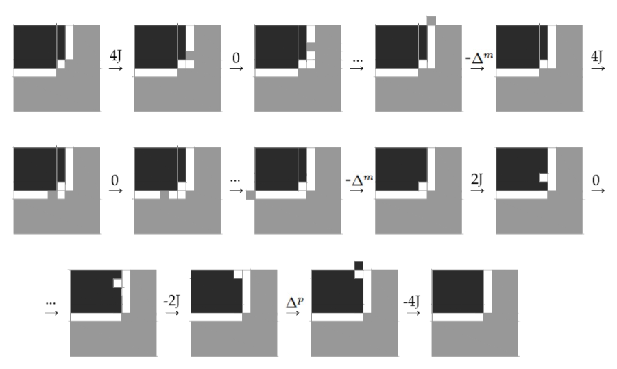
Figure 13: In this part of the reference path, a frame in the corner with side lengths $l$ and $l+1$ is created.

We repeat this mechanism of growing of the frame in the corner along the shortest side, until we reach the homogeneous phase ${\boldsymbol{+1}}$.

In order to find the energy barrier to reach ${\boldsymbol{+1}}$ starting from ${\boldsymbol{-1}}$, we compute the value of the maximal energy of $\sigma_{n,m}$ and we sum to it the value in (3.33). The energy of $\sigma_{n,m}$ with $m,n\in\mathbb{N}$ respect to the energy of the homogeneous state ${\boldsymbol{-1}}$ is

$$H(\sigma_{n,m})-H({\boldsymbol{-1}})=2J(n+m)+\lambda(n+m)-h(2nm+n+m).$$ (3.34)

The maximal value of this function is attained for $n=m=\frac{2J+\lambda-h}{2h}$, however $n$ and $m$ are integer number, so with a simple computation we find that the chopped corner frame with maximal energy has size $l_{c}=\lfloor\frac{2J+\lambda-h}{2h}\rfloor+1$ and $l_{c}-1$. Thus, the height along the reference path is reached in a configuration $\sigma_{s}$ obtained as $\eta$, see as Figure 2, and its value is equal to

$$H(\sigma_{s})-H({\boldsymbol{-1}}) =2J(2l_{c}-1)+\lambda(2l_{c}-1)-h(2l_{c}^{2}-1)+6J+2(\lambda-h)-2(\lambda+h)$$

$$=4J(l_{c}+1)+\lambda(2l_{c}-1)-h(2l_{c}^{2}+3)$$ (3.35)

and then

$$V_{{\boldsymbol{-1}}}\leq H(\sigma_{s})-H({\boldsymbol{-1}}).$$ (3.36)

3.6.2 Lower bound for $V_{{\boldsymbol{-1}}}$

In order to find the lower bound for $V_{\boldsymbol{-1}}$, we use [15, Lemma 4.14], that we report here for the convenience of the reader. Let $n^{+}_{c}=l_{c}(l_{c}-1)$ and denote by $\mathcal{M}_{n^{+}_{c}}\subset\mathcal{X}$ (resp. $\mathcal{M}_{n^{+}_{c}+1}\subset\mathcal{X}$) the manifold with fixed number $n^{+}_{c}$ (resp. $n^{+}_{c}+1$) of pluses. We recall, the definition of the configuration $\sigma_{c}=\sigma_{l_{c}-1,l_{c}}$ provided in Figure 2.

Lemma 3.14.

$H(\sigma_{c})=\min_{\xi\in\mathcal{M}_{n^{+}_{c}}}H(\xi)$.

Note that this lemma was proven in [15] for the Blume-Capel model, with the Hamiltonian (2.3) that we use in this paper, with the Glauber dynamics. We remark that the result is valid also in this setting, since it does not depend on the dynamics but only on the structure of the Hamiltonian.

Consider $\underline{\omega}$ from ${\boldsymbol{-1}}$ to ${\boldsymbol{+1}}$ and let $\sigma\in\mathcal{M}_{n^{+}_{c}}$ and $\eta\in\mathcal{M}_{n^{+}_{c}+1}$ be two consecutive configurations along this path. Then $\Phi(\underline{\omega})\geq H(\eta)=H(\sigma)+\Delta^{p}$. By Lemma 3.14, we have $H(\sigma)\geq H(\sigma_{c})$ and therefore $V_{{\boldsymbol{-1}}}\geq H(\sigma_{c})+\Delta^{p}-H({\boldsymbol{-1}})$.

3.7 Proof of Theorem 2.3

By (2.7) it follows that $V^{*}<H(\sigma_{c})+\Delta^{p}-H({\boldsymbol{-1}})$. Thus, by Theorems 2.1 and 2.2 it follows that the stability level of ${\boldsymbol{-1}}$ is larger that the stability level of all other configurations differing from ${\boldsymbol{+1}}$.

Since, the stability level of ${\boldsymbol{-1}}$ is the maximal one for the configurations in $\mathcal{X}\setminus\{{\boldsymbol{-1}}\}$, by [16, Theorem 2.4] we have that ${\boldsymbol{-1}}$ is the unique metastable state for the system.

3.8 Proof of Theorem 2.4

Remark that $V_{\boldsymbol{-1}}$ is the maximal stability level. Then, by applying [31, Theorem 4.1] with $\eta_{0}={\boldsymbol{-1}}$ we get that

$$\lim_{\beta\to\infty}\mathbb{P}_{{\boldsymbol{-1}}}(e^{\beta(V_{\boldsymbol{-1}}-\epsilon)}<\tau_{{\boldsymbol{+1}}}<e^{\beta(V_{\boldsymbol{-1}}+\epsilon)})=1,$$

for any $\epsilon>0$. Thus the theorem follows by noting that the event $\{e^{\beta(V_{\boldsymbol{-1}}-\epsilon)}<\tau_{{\boldsymbol{+1}}}<e^{\beta(V_{\boldsymbol{-1}}+\epsilon)}\}$ is a subset of the event $\{e^{\beta(H(\sigma_{c})+\Delta^{p}-H({\boldsymbol{-1}})-\epsilon)}<\tau_{{\boldsymbol{+1}}}<e^{\beta(H(\sigma_{s})-H({\boldsymbol{-1}})+\epsilon)}\}$.

4 Proof of lemmas

In this section we prove all the auxiliary lemmas related to the recurrence property and stated in Section 3.4.

Proof of Lemma 3.4.

Before starting the proof, we recall that a complete weighted directed graph $G=(V,E)$ is a graph such that a weight $w{(u,v)}$ is associated to every edge $(u,v)$ of the graph and every vertex is connected with the others. Moreover, given a path $p$ on $G$, the sum of the weights along the path is called path-weight and denoted by $w_{p}$. Given a path $p=(v_{1},...,v_{n})$, the maximal sub-path weight is defined as $m_{p}=\max_{k\in\{1,...,n-1\}}\sum_{i=1}^{k}w(v_{i},v_{i+1})$.

Let $\sigma\in\mathcal{X}$ be a configuration as in the assumption. In particular, we suppose that $\sigma$ contains a zero-carpet. The proof of the other cases is analogous.

We let $x_{0}:=x$ and let $x_{1},...,x_{n}$ be a sequence of sites of $X^{\prime}$ such that $x_{i}$ is connected with $x_{i+1}$ for $i=0,...,n-1$. Recall $\sigma(x)=r\in\{-1,+1\}$.

We consider a weighted directed graph $G=(V,E)$ with self-loops such that each vertex is a non-ordered pair of spins and it is connected with all the others. Each weight $w(v,u)$ is defined as reported in Figure 3.

We associate to every site $x_{i}$ of the sequence $x_{0},x_{1},...,x_{n}$ a vertex in $V$ such that the nearest sites of $x_{i}$ different from $x_{i-1}$ and $x_{i+1}$ have spins equal to the vertex. We denote by $v_{i}$ the vertex associated with $x_{i}$. We recall that the sites $x_{0},x_{1},...,x_{n}$ have two nearest spins equal to zero.

We consider $x_{i},x_{j}$ as above and we note that $H(\sigma^{(x,x_{j})})-H(\sigma^{(x,x_{i})})$ is equal to the weight $w(v_{i},v_{j})$; for the sake of clarity the weight already reported in the left panel of Figure 3 are reported also in 4.1.

Table 4.1: Energy difference for all the possible choices of the local configuration of the sites $x$ and $y$ zeros after the swap of the particle originally at site $x$. The two neighbouring spins not specified in the table are zeros.

We consider a path from $\sigma^{(x,x_{i})}$ to $\sigma^{(x,x_{j})}$ composed by the following pairwise communicating configurations $\underline{\omega}=(\sigma^{(x,x_{i})},\sigma^{(x,x_{i+1})},...,\sigma^{(x,x_{j-1})},\sigma^{(x,x_{j})})$. In order to compute the height of this path, we consider the associated path $p_{\underline{\omega}}$ on the graph $G$ and we compute its maximal sub-path weight.

In the following, we explain in detail how to compute the maximal sub-path weight of a general path $p$ on $G$. First, we consider the path $p^{\prime}$ obtained removing all the loops in $p$. We note that the path-weight of a loop is $0$, because the weight of the edge $(v,u)$ is defined as the difference of a real-valued function $f$ calculated in the two vertices $v$ and $u$, i.e. $w(v,u)=f(v)-f(u)$. Hence, it follows that $w(v,u)=-w(u,v)$ for each pair of vertices $v,u$. Moreover, from Figure 3, the maximal sub-path weight of $p$ is smaller than or equal to $8J$. Thus, $\Phi_{\underline{\omega}}a=m_{p_{\underline{\omega}}}\leq 8J$.

∎

Proof of Lemma 3.5.

(i). Let $\sigma$ be a configuration as in the assumption and let $\eta=\sigma^{(x;s)}$. Let $s\in\{-1,+1\}$. Let $x_{1},...,x_{n}\in X$ and $x_{0}\in\partial^{+}\Lambda_{0}$ such that $|x_{i}-x_{i-1}|=1$ for $i=1,...,n$ and $|x_{n}-x|=1$. We construct a path $\underline{\omega}=(\sigma,\omega_{0},\omega_{1},...,\omega_{n},\eta)$ in the following way:

$$\omega_{0}:=\sigma^{(x_{0};s)};\qquad\omega_{i}:=\omega_{i-1}^{(x_{i-1},x_{i})}\text{ for }i=1,...n;\qquad\omega_{n+1}:=\omega_{n}^{(x_{n},x)}.$$ (4.37)

We observe that $\omega_{n+1}=\eta$. By (2.3) and (2.12), we have

$$H(\eta)-H(\sigma) =[H(\eta)-H(\omega_{0})]+[H(\omega_{0})-H(\sigma)]$$

$$\leq 2J\Big{[}[D_{x}(\omega_{0})+D_{x_{0}}(\omega_{0})]-[D_{x}(\eta)+D_{x_{0}}(\eta)]\Big{]}+\Delta_{s}=-2JD_{x}(\eta)+\Delta_{s},$$ (4.38)

where the equality holds when $\sigma(x_{0})=0$. We compute now the height between $\sigma$ and $\sigma^{(x;s)}$ along the path $\underline{\omega}$. We get the particle $s$ in $\partial^{+}\Lambda_{0}$ if $\sigma(x)\neq s$, and the energy increases at most by $\Delta_{s}$, i.e. $H(\omega_{0})\leq H(\sigma)+\Delta_{s}$. By applying Lemma 3.4 to $\omega_{0}$, we have

$$\Phi((\omega_{0},...,\omega_{n}))\leq H(\omega_{0})+8J\leq H(\sigma)+\Delta_{s}+8J.$$ (4.39)

Thus,

$$\Phi((\sigma,...,\eta)) =\max\{\Phi((\omega_{0},...,\omega_{n})),\Phi((\omega_{n},\eta))\}$$

$$\leq H(\sigma)+\Delta_{s}+8J+2J|D_{x}(\eta)|\leq H(\sigma)+18J.$$ (4.40)

(ii). Let $\sigma$ be a configuration as in the assumption. We let $x_{0}=x$ and $\sigma(x)=s\neq 0$. Let $x_{1},...,x_{n}\in X$ and $x_{n}\in\partial^{+}\Lambda_{0}$ such that $|x_{i}-x_{i-1}|=1$ for $i=1,...,n$. We construct a path $\underline{\omega}=(\sigma,\omega_{0},\omega_{1},...,\omega_{n},\eta)$ in the following way:

$$\omega_{0}:=\sigma;\qquad\omega_{i}:=\omega_{i-1}^{(x_{i-1},x_{i})}\text{ for }i=1,...,n;\qquad\omega_{n+1}=\sigma^{(x;0)}.$$ (4.41)

By (2.3) and (2.12), we obtain

$$H(\omega_{n})-H(\sigma)=2JD_{x}(\sigma),$$

$$H(\omega_{n+1})-H(\omega_{n})=-\Delta_{s}$$ (4.42)

Moreover, $\Phi((\omega_{n},\omega_{n+1}))=H(\omega_{n})$ since $H(\omega_{n+1})<H(\omega_{n})$, and by applying Lemma 3.4 to $\omega_{1}$ we have that

$$\Phi((\omega_{1},...,\omega_{n}))\leq H(\omega_{1})+8J\leq H(\omega_{0})+2J|D_{x_{0},x_{1}}(\omega_{0})|+8J,$$ (4.43)

Thus, we have

$$\Phi((\omega_{0},\omega_{n+1})) \leq\max\{\Phi((\omega_{0},\omega_{1})),\Phi((\omega_{1},...,\omega_{n}))\}$$

$$=\max\{H(\omega_{0})+2J|D_{x_{0},x_{1}}(\omega_{0})|,H(\omega_{0})+2J|D_{x_{0},x_{1}}(\omega_{0})|+8J\}\leq H(\omega_{0})+14J,$$ (4.44)

where the last inequality follows from the fact that in the worst case $x_{0}$ has three nearest neighbours with spin equal to $s$ and the two nearest neighbours of $x_{1}$ not in $X$ has spin value $-s$. ∎

Proof of Lemma 3.6.

(i). Let $\sigma$ be a configuration as in the assumption and let $\eta=\sigma^{(y;0)}$. We suppose first $\sigma(y)=-s$. Set $y_{0}=y$ and let $y_{1},...,y_{n}\in X$ be such that $|y_{i}-y_{i-1}|=1$ for $i=1,...,n$ and $y_{n}\in\partial^{-}\Lambda_{0}$. Let $z\in\partial^{+}\Lambda_{0}$ be at distance one from $X$ and, without loss of generality, we assume that $\sigma(z)=0$. We construct a path $\underline{\omega}$ from $\sigma$ to $\eta$ in the following way:

• the particle with spin $-s$ in $y$ moves through the s-carpet until $\partial^{-}\Lambda_{0}$;

• the $-s$ in $\partial^{-}\Lambda_{0}$ is exchanged with a zero in $\partial^{+}\Lambda_{0}$ and then it leaves $\Lambda$;

• the zero in $\partial^{-}\Lambda_{0}$ moves along the s-carpet until it reaches the site $y$.

Formally, we define the path $\underline{\omega}=(\omega_{0},\omega_{1},\omega_{n},\omega_{n+1},\xi_{0},\xi_{1},...,\xi_{n})$ such that

$$\omega_{0}:=\sigma;\qquad \omega_{i}:=\omega_{i-1}^{(y_{i-1},y_{i})}\text{ for }i=1,...n;\qquad\,\,\,\omega_{n+1}:=\omega_{n}^{(y_{n},z)};$$ (4.45)

$$\xi_{0}:=\omega_{n+1}^{(z;0)};\qquad \xi_{i}:=\xi_{i-1}^{(y_{n-i+1},y_{n-i})}\text{ for }i=1,...,n.$$ (4.46)

We note that $\xi_{n}=\eta$. By (2.3) and (2.12), we obtain

$$H(\eta)-H(\sigma)=2JD_{y}(\sigma)-\Delta_{-s}$$ (4.47)

Next, we compute the height between $\sigma$ and $\eta$ along this path.

$$\Phi(\underline{\omega})=\max\{ \Phi((\sigma,\omega_{1})),\,\Phi((\omega_{1},...,\omega_{n-1})),\,\Phi((\omega_{n-1},\omega_{n},\omega_{n+1})),\,\Phi((\omega_{n+1},\xi_{0})),\Phi((\xi_{0},\xi_{1})),$$

$$\Phi((\xi_{1},...,\xi_{n-1})),\,\Phi((\xi_{n-1},\eta))\}$$

We note that $\Phi((\sigma,\omega_{1}))=\max\{H(\sigma),H(\omega_{1})\}\leq H(\sigma)+2J|D_{y_{0},y_{1}}(\sigma)|$, and by applying Lemma 3.4 to the configuration $\omega_{1}$ we have that

$$\Phi((\omega_{1},...,\omega_{n-1}))\leq H(\omega_{1})+16J\leq H(\sigma)+2J|D_{y_{0},y_{1}}(\sigma)|+16J$$ (4.48)

Then, $\Phi((\sigma,\omega_{1}))\leq\Phi((\omega_{1},...,\omega_{n-1}))$. Moreover, $\Phi((\omega_{n+1},\xi_{0}))=H(\omega_{n+1})$ since $H(\xi_{0})<H(\omega_{n+1})$, then $\Phi((\omega_{n+1},\xi_{0}))\leq\Phi((\omega_{n-1},\omega_{n},\omega_{n+1}))=\max\{H(\omega_{n-1}),H(\omega_{n}),H(\omega_{n+1})\}$ and

$$H(\omega_{n+1})=H(\omega_{n})+2JD_{y_{n},z}(\omega_{n})$$

$$H(\omega_{n})=H(\omega_{n-1})+2JD_{y_{n-1},y_{n}}(\omega_{n-1})$$

$$H(\omega_{n-1})\leq H(\omega_{1})+16J$$ (4.49)

where the last inequality follows from Lemma 3.4. Then,

$$\Phi((\omega_{n-1},\omega_{n},\omega_{n+1})) \leq H(\omega_{1})+2J|D_{y_{n},z}(\omega_{n})|+2J|D_{y_{n-1},y_{n}}(\omega_{n-1})|+16J$$

$$\leq H(\sigma)+2J|D_{y_{0},y_{1}}(\sigma)|+2J|D_{y_{n},z}(\omega_{n})|+2J|D_{y_{n-1},y_{n}}(\omega_{n-1})|+32J$$ (4.50)

Thus

$$\max\{\Phi((\sigma,\omega_{1})),\Phi((\omega_{1},...,\omega_{n-1})),\Phi((\omega_{n-1},\omega_{n},\omega_{n+1}))\}\leq H(\sigma)+54J,$$ (4.51)

since $2J|D_{y_{0},y_{1}}(\sigma)|\leq 10J$, $2J|D_{y_{n},z}(\omega_{n})|\leq 4J$ and $2J|D_{y_{n-1},y_{n}}(\omega_{n-1})|\leq 8J$.

Furthermore, $\Phi((\xi_{0},\xi_{1}))=\max\{H(\xi_{0}),H(\xi_{1})\}\leq H(\xi_{0})+2J|D_{y_{n},y_{n-1}}(\xi_{0})|$, and by applying Lemma 3.4 to $\xi_{1}$ we have that

$$\Phi((\xi_{1},...,\xi_{n-1}))\leq H(\xi_{1})+8J\leq H(\xi_{0})+2J|D_{y_{n},y_{n-1}}(\xi_{0})|+8J,$$ (4.52)

then $\Phi((\xi_{0},\xi_{1}))\leq\Phi((\xi_{1},...,\xi_{n-1}))$. Finally,

$$\Phi((\xi_{n-1},\xi_{n}))=\max\{H(\xi_{n-1}),H(\xi_{n})\} \leq H(\xi_{n-1})+2J|D_{y_{1},y_{0}}(\xi_{n-1})|$$

$$\leq H(\xi_{1})+8J+2J|D_{y_{1},y_{0}}(\xi_{n-1})|$$

$$\leq H(\xi_{0})+2J|D_{y_{n},y_{n-1}}(\xi_{0})|+8J+2J|D_{y_{1},y_{0}}(\xi_{n-1})|$$ (4.53)

where the second inequality is obtained by using Lemma 3.4. Then,

$$\max\{\Phi((\xi_{0},\xi_{1})),\Phi((\xi_{1},...,\xi_{n-1})),\Phi((\xi_{n-1},\xi_{n}))\}\leq H(\xi_{0})+26J,$$ (4.54)

since $2J|D_{y_{n},y_{n-1}}(\xi_{0})|\leq 8J$ and $2J|D_{y_{1},y_{0}}(\xi_{n-1})|\leq 10J$.

Thus, by (4.51) and (4.54), we obtain

$$\Phi((\sigma,...,\xi_{n})) \leq\max\{H(\sigma)+54J,\,H(\xi_{0})+26J\}.$$ (4.55)

Moreover

$$H(\xi_{0})-H(\sigma) =[H(\xi_{0})-H(\omega_{n+1})]+[H(\omega_{n+1})-H(\omega_{n})]+[H(\omega_{n})-H(\sigma)]$$

$$=-\Delta_{-s}+2J|D_{y_{n},z}(\omega_{n})|+2J|D_{y_{0},y_{n}}(\sigma)|$$

$$\leq-\Delta_{-s}+14J<10J+(\lambda-sh)<11J$$ (4.56)

since $2J|D_{y_{n},z}(\omega_{n})|\leq 4J$, $2J|D_{y_{0},y_{n}}(\sigma)|\leq 10J$ and Condition 2.7. Thus, we conclude

$$\Phi((\sigma,...,\omega_{n+1}))\leq H(\sigma)+54J.$$ (4.57)

In the case of $\sigma(y)=s$, we proceed in a similar way by constructing a path from $\sigma$ to $\eta$ composed by only the last part of the previous path. i.e. starting from $\sigma$ the zero in $\partial^{-}\Lambda_{0}$ moves along the s-carpet until it reaches the site $y$.

(ii). Let $\sigma$ be a configuration as in the assumption, and let $\eta=\sigma^{(y;s)}$. Set $y=y_{0}$ and let $y_{1},...,y_{n}\in X$ be such that $|y_{i}-y_{i-1}|=1$ for $i=1,...,n$ and $y_{n}\in\partial^{-}\Lambda_{0}$. Let $z\in\partial^{+}\Lambda_{0}$ and we construct a path $\underline{\omega}$ from $\sigma$ to $\eta$ in the following way:

• the particle with zero spin in $y$ crosses the s-carpet until $y_{n}\in\partial^{-}\Lambda_{0}$;

• a particle with spin $s$ gets in $\partial^{+}\Lambda_{0}$;

• the particle moves from $z$ to $y_{n}$ by exchanging with the zero in $y_{n}$.

Formally, we define the path $\underline{\omega}=(\omega_{0},\omega_{1},\omega_{n},\omega_{n+1},\xi_{0},\xi_{1},...,\xi_{n})$ such that

$$\omega_{0}:=\sigma;\qquad\qquad\omega_{i}:=\omega_{i-1}^{(y_{i-1},y_{i})}\text{ for }i=1,...n;$$ (4.58)

$$\xi_{1}:=\omega_{n}^{(z;s)};\qquad\,\,\xi_{2}:=\omega_{n+1}^{(z,y_{n})}.$$ (4.59)

We note that $\xi_{2}=\eta$. By (2.3) and (2.12), we obtain

$$H(\eta)-H(\sigma)=[H(\eta)-H(\xi_{1})]+[H(\xi_{1})-H(\sigma)]=-2JD_{y}(\eta)+\Delta_{s}$$ (4.60)

Next, we compute the height between $\sigma$ and $\eta$ along this path.

$$\Phi(\underline{\omega})=\max\{\Phi((\sigma,\omega_{1})),\,\Phi((\omega_{1},...,\omega_{n-1})),\,\Phi((\omega_{n-1},...,\eta)),\}$$

We note that $\Phi((\sigma,\omega_{1}))=\max\{H(\sigma),H(\omega_{1})\}\leq H(\sigma)+2J|D_{y_{0},y_{1}}(\sigma)|$, and by applying Lemma 3.4 to the configuration $\omega_{1}$ we have that

$$\Phi((\omega_{1},...,\omega_{n-1}))\leq H(\omega_{1})+8J\leq H(\sigma)+2J|D_{y_{0},y_{1}}(\sigma)|+8J\leq H(\sigma)+18J$$ (4.61)

since $2J|D_{y_{0},y_{1}}(\sigma)|\leq 10J$. Then, $\Phi((\sigma,\omega_{1}))\leq\Phi((\omega_{1},...,\omega_{n-1}))$.

Moreover, $\Phi((\omega_{n-1},...,\eta))=\max\{H(\omega_{n-1}),H(\omega_{n}),H(\xi_{1}),H(\eta)\}$ and

$$H(\eta)=H(\xi_{1})+2JD_{z,y_{n}}(\xi_{1})\leq H(\xi_{1})+4J$$

$$H(\xi_{1})=H(\omega_{n})+\Delta_{s}$$

$$H(\omega_{n})=H(\omega_{n-1})+2JD_{y_{n-1},y_{n}}(\omega_{n-1})\leq H(\omega_{n-1})+8J$$

$$H(\omega_{n-1})\leq H(\omega_{1})+8J$$ (4.62)

where the last inequality follows from Lemma 3.4. Then,

$$\Phi((\omega_{n-1},...,\eta))\leq H(\omega_{1})+\Delta_{s}+20J\leq H(\omega_{1})+25J\leq H(\sigma)+2J|D_{y_{0},y_{1}}(\sigma)|+25J\leq H(\sigma)+35J$$ (4.63)

Thus, by (4.61) and (4.63), we conclude $\Phi((\sigma,...,\eta))\leq H(\sigma)+35J$.

∎

Proof of Lemma 3.7.

Let $\sigma$ be a configuration as in the assumption. Suppose that $\sigma_{\partial^{+}\Lambda_{0}}=0_{\partial^{+}\Lambda_{0}}$, otherwise the stability level of $\sigma$ is zero, indeed when a plus or a minus leaves $\Lambda$ the energy decreases. Assume first that the bond $(+,-)$ is at distance one from $\partial^{+}\Lambda_{0}$. We consider the configuration $\eta=\sigma^{(x;0)}$ where $x$ is the site of the bond at distance one from $\partial^{+}\Lambda_{0}$. Suppose without loss of generality that $\sigma(x)=-1$, then with a direct computation we have

$$H(\eta)-H(\sigma)\leq-2J+(\lambda-h)<0.$$ (4.64)

We note that $\sigma$ and $\eta$ are not communicating configurations. Let $\xi=\sigma^{(x,x^{\prime})}$ where $x^{\prime}\in\partial^{+}\Lambda_{0}$ is at distance one from $x$, then $\sigma\sim\xi\sim\eta$ and

$$\Phi(\sigma,\eta)-H(\sigma)=\max\{H(\xi)-H(\sigma),0\}\leq 2J,$$ (4.65)

since $D_{x}(\sigma)\leq 1$, where $D_{x}(\sigma)$ is defined in (2.11).

In the following, assume that there exists a zero–carpet at distance one from $x$, where $x$ is one of the two sites of the bond. Suppose without loss of generality that $\sigma(x)=-1$. We apply Lemma 3.5-(ii) and we obtain

$$\Phi(\sigma^{(x;0)},\sigma)-H(\sigma)\leq 14J\qquad\text{ and }\qquad H(\sigma^{(x;0)})-H(\sigma)\leq-2J+(\lambda-h),$$ (4.66)

since this minus spin is at distance one from a plus spin and a zero spin of the carpet, then it has at most two nearest neighbors with the same value of the spin. This implies that $D_{x}(\sigma)\leq 1$, where $D_{x}(\sigma)$ is defined in (2.11). ∎

Proof of Lemma 3.8.

Let $\sigma$ as in the assumption. Suppose that $\sigma_{\partial^{+}\Lambda_{0}}=0_{\partial^{+}\Lambda_{0}}$, otherwise $V_{\sigma}=0$, indeed when a plus or a minus leaves $\Lambda$ the energy decreases. Suppose without loss of generality that $s=-1$ and that the plus belonging to the bond $(+,-)$ is at distance one from the minus-carpet. We consider the configuration $\sigma^{(x;0)}$, where $x$ is the site of the bond with plus spin. Assume first that this plus has at most two pluses as nearest neighbours, then by using Lemma 3.6-(i), we have

$$\Phi(\sigma,\sigma^{(x;0)})-H(\sigma)\leq 54J\qquad\text{ and }\qquad H(\sigma^{(x;0)})-H(\sigma)\leq-2J+(\lambda+h).$$ (4.67)

Now, we suppose that this plus spin has three pluses as nearest neighbours. We analyze the two columns (or rows) that contains the bond $(+,-)$ until we possibly find a bond different from $(+,-)$. In the case that $\sigma$ contains two columns composed by all bonds $(+,-)$ in $\Lambda_{0}$, we look at the bond of these two columns in $\partial^{-}\Lambda_{0}$ and we note that the plus of this bond has at most two nearest neighbours equal to plus, so we proceed as before. In the case that there exists a bond different from $(+,-)$ in the two columns, we distinguish two cases: (i) if the pair of spins in the bond is of the type $(s,r)$ with $s\neq+1$ and $r\in\{-1,0,+1\}$, then the nearest bond $(+,-)$ contains a plus with at most two pluses nearest neighbours and we proceed as before; (ii) if the pair of spins in the bond is of the type $(+,r)$, then the nearest bond $(+,-)$ contains a minus with at most two minus nearest neighbours and we conclude by applying Lemma 3.6-(i) to this minus. ∎

Proof of Lemma 3.9.

Let $\sigma$ be a configuration as in the assumption. Suppose that $\sigma_{\partial^{+}\Lambda_{0}}=0_{\partial^{+}\Lambda_{0}}$, otherwise $V_{\sigma}=0$, indeed when a plus or a minus leaves $\Lambda$ the energy decreases. Assume first $\sigma(x_{4})\neq-1$ and we consider the configuration $\eta=\sigma^{(x;+)}$. Then, we conclude by applying Lemma 3.5-(i). On the other hand, we suppose $\sigma(x_{4})=-1$ with at most two nearest neighbors equal to $-1$. We apply Lemma 3.5-(ii) to $x_{4}$ and we obtain a configuration $\xi=\sigma^{(x_{4};0)}$ such that $\Phi(\sigma,\xi)\leq H(\sigma)+14J$ and $H(\xi)\leq H(\sigma)+(\lambda-h)$. The configuration $\xi$ satisfies the assumption of Lemma 3.5-(i), thus we define the configuration $\eta=\xi^{(x;+)}$ such that $\Phi(\xi,\eta)\leq H(\xi)+18J$ and $H(\eta)\leq H(\xi)-(\lambda+h)$. Then, $H(\eta)<H(\sigma)$ and finally $\Phi(\sigma,\eta)\leq\max\{\Phi(\sigma,\xi),\Phi(\xi,\eta)\}\leq 18J.$ ∎

Proof of Lemma 3.10.

Let $\sigma_{0}=\sigma$ be a configuration that contains a cluster of pluses as in the assumption. The proof for a cluster of minuses is similar. Suppose that $\sigma_{\partial^{+}\Lambda_{0}}=0_{\partial^{+}\Lambda_{0}}$, otherwise $V_{\sigma}=0$, indeed when a plus or a minus leaves $\Lambda$ the energy decreases. We call $x_{1},...,x_{l}$ the sites along the convex side of the cluster and let $x_{1}$ be the corner along this side at distance one from the zero-carpet. We define a path between $\sigma_{0}$ and the configuration $\sigma_{l}$ obtained from $\sigma_{0}$ by shrinking the cluster of pluses, formally:

$$\sigma_{i}=\sigma_{i-1}^{(x_{i};0)}\text{ for }i=1,...,l.$$ (4.68)

We note that these configurations are not communicating, so we construct a path from $\sigma_{i-1}$ to $\sigma_{i}$ for every $i=1,...,l$ in the following way. For $i=1$, the plus in $x_{1}$ moves along the zero-carpet until $\partial^{+}\Lambda_{0}$ and then it leaves $\Lambda$. By using Lemma 3.5-(i), we have $H(\sigma_{1})-H(\sigma_{0})\leq\lambda+h$ and $\Phi(\sigma_{0},\sigma_{1})\leq H(\sigma_{0})+14J$. For $i=2$, the plus in $x_{2}$ is at distance one from the zero-carpet in $\sigma_{1}$ obtained by adding the zero in $x_{1}$ to the zero-carpet in $\sigma_{0}$, then it moves along the zero-carpet until $\partial^{+}\Lambda_{0}$ and then it leaves $\Lambda$. As before, by using Lemma 3.5-(i), we have $H(\sigma_{2})-H(\sigma_{1})\leq\lambda+h$ and $\Phi(\sigma_{1},\sigma_{2})\leq H(\sigma_{1})+14J$. Thus,

$$\Phi(\sigma_{0},\sigma_{2})=\max\{\Phi(\sigma_{0},\sigma_{1}),\Phi(\sigma_{1},\sigma_{2})\}\leq H(\sigma_{1})+14J\leq H(\sigma_{0})+(\lambda+h)+14J$$ (4.69)

We iterate this procedure for every $i=3,...,l-1$ and we obtain $H(\sigma_{l-1})-H(\sigma_{l-2})\leq\lambda+h$ and $\Phi(\sigma_{l-2},\sigma_{l-1})\leq H(\sigma_{l-2})+14J$. Thus,

$$\Phi(\sigma_{0},\sigma_{l-1}) =\max\{\Phi(\sigma_{0},\sigma_{1}),\Phi(\sigma_{1},\sigma_{2}),...,\Phi(\sigma_{l-2},\sigma_{l-1})\}$$

$$\leq H(\sigma_{l-2})+14J\leq H(\sigma_{0})+(l-1)(\lambda+h)+14J.$$ (4.70)

When the last plus in $x_{l}$ is detached from the cluster of pluses and it leaves $\Lambda$, by using Lemma 3.5-(i), we have $H(\sigma_{l})-H(\sigma_{l-1})\leq-2J+\lambda+h$ and $\Phi(\sigma_{l-1},\sigma_{l})\leq H(\sigma_{l-1})+14J\leq\Phi(\sigma_{l-2},\sigma_{l-1})$. Then, we have

$$H(\sigma_{l})\leq H(\sigma_{0})-2J+l(\lambda+h)<H(\sigma_{0}),$$ (4.71)

where the last inequality follows from the assumption $l\leq\lfloor\frac{2J}{\lambda+h}\rfloor$, and

$$\Phi(\sigma_{0},\sigma_{l})\leq H(\sigma_{0})+(l-1)(\lambda+h)+14J<H(\sigma_{0})+16J.$$ (4.72)

∎

Proof of Lemma 3.11.

Let $\sigma_{0}=\sigma$ be a configuration that contains a cluster of pluses as in the assumption. The proof for a cluster of minuses is similar. Suppose that $\sigma_{\partial^{+}\Lambda_{0}}=0_{\partial^{+}\Lambda_{0}}$, otherwise $V_{\sigma}=0$, indeed when a plus or a minus leaves $\Lambda$ the energy decreases. If there is at least a plus spin at distance strictly smaller than two from the convex side, then we conclude by applying Lemma 3.5-(ii). Otherwise, all sites at distance smaller than two are zeros and we define a path between $\sigma_{0}$ and the configuration $\sigma_{l}$ obtained from $\sigma_{0}$ by adding a strip of pluses with length $l$ to the cluster of pluses. More precisely, we can call $x_{1},...,x_{l}$ the sites at distance one from the convex side that form a strip of zeros in such a way that the transition from $\sigma_{0}$ to $\sigma_{l}$ can be realized through the following sequence of configurations:

$$\sigma_{i}=\sigma_{i-1}^{(x_{i};+)}\text{ for }i=1,...,l.$$ (4.73)

We note that these configurations are not communicating, so we create a path from $\sigma_{i-1}$ to $\sigma_{i}$ for every $i=1,...,l$ in the following way. For $i=1$, a plus gets in $\partial^{+}\Lambda_{0}$ and it moves along the zero-carpet until $x_{1}$. By using Lemma 3.5-(i), we have $H(\sigma_{1})-H(\sigma_{0})\leq 2J-(\lambda+h)$ and $\Phi(\sigma_{0},\sigma_{1})\leq H(\sigma_{0})+18J$. For $i=2$, another plus gets in $\partial^{+}\Lambda_{0}$ and it moves along the zero-carpet until in $x_{2}$. By using Lemma 3.5-(i), we have $H(\sigma_{2})-H(\sigma_{1})\leq 2J-(\lambda+h)$ and $\Phi(\sigma_{1},\sigma_{2})\leq H(\sigma_{1})+18J$, note that the $2J$ in the estimate of the energy difference is not present if $x_{1}$ and $x_{2}$ are nearest neighbours. Thus,

$$\Phi(\sigma_{0},\sigma_{2})=\max\{\Phi(\sigma_{0},\sigma_{1}),\Phi(\sigma_{1},\sigma_{2})\}\leq H(\sigma_{1})+18J\leq H(\sigma_{0})+22J-(\lambda+h)$$ (4.74)

We iterate this procedure for every $i=3,...,l-1$. We stress that from $i=3$ on each new plus spin will be accommodated at a site with at least two neighboring pluses, so that $H(\sigma_{i})-H(\sigma_{i-1})\leq-(\lambda+h)$ and $\Phi(\sigma_{i-1},\sigma_{i})\leq H(\sigma_{i-1})+18J$. Thus, $\Phi(\sigma_{i-1},\sigma_{i})\leq\Phi(\sigma_{i-2},\sigma_{i-1})$, since $H(\sigma_{i})<H(\sigma_{i-1})$ for $i=1,...,l$. Then,

$$\Phi(\sigma_{0},\sigma_{l}) =\max\{\Phi(\sigma_{0},\sigma_{1}),\Phi(\sigma_{1},\sigma_{2}),...,\Phi(\sigma_{l-1},\sigma_{l})\}$$

$$=\max\{\Phi(\sigma_{0},\sigma_{1}),\Phi(\sigma_{1},\sigma_{2})\}<H(\sigma_{0})+22J.$$ (4.75)

Finally, we conclude

$$H(\sigma_{l})-H(\sigma_{0})\leq H(\sigma_{0})+2J-l(\lambda+h)<H(\sigma_{0}),$$ (4.76)

since $l\geq\lfloor\frac{2J}{\lambda+h}\rfloor+1$. ∎

Proof of Lemma 3.12.

Let $\sigma$ be a configuration as in the assumption. Suppose that $\sigma_{\partial^{+}\Lambda_{0}}=0_{\partial^{+}\Lambda_{0}}$, otherwise $V_{\sigma}=0$, indeed when a plus or a minus leaves $\Lambda$ the energy decreases. Let $l$ be the length of the strip of pluses. We distinguish two cases:

• Consider the flag-shaped structure in the right panel of Figure 4.

• Consider the flag-shaped structure in the left panel of Figure 4.

We start with the case (i). Assume first $l\geq\lfloor\frac{2J}{h}+\frac{\lambda-h}{h}\rfloor$+1.

Let $x_{1},...,x_{l}$ be the sites in the flag-shaped structured with minus spin and such that $|x_{i}-x_{i+1}|=1$ for every $i=1,...,l-1$. Let $y_{1},...,y_{l}$ be the sites in the flag-shaped structured with zero spin and such that $|y_{i}-x_{i}|=1$ for every $i=1,...,l$. Let $z_{1}$ and $z_{2}$ be the two sites outside the flag-shaped structured such that $\sigma(z_{1})=\sigma(z_{2})=-1$, $|z_{1}-y_{1}|=1$ and $|z_{2}-y_{l}|=1$.

First, we note that if $z_{1}$, $z_{2}$ have three nearest neighbours with minus spin, then there exists a bond $(+,-)$ and we conclude by applying Lemma 3.8. Then, assume that $z_{1}$ and $z_{2}$ have at most two nearest neighbours with minus spins. Moreover, we suppose that $z_{j}$ and $x_{i}$ for every $j=1,2$ and every $i=1,...,l$ have only nearest neighbours with minus or zero spins, otherwise we conclude by applying Lemma 3.8.

We construct a path from $\sigma$ to $\sigma_{2l+2}$ where $\sigma_{2l+2}$ is such that

$$\sigma_{2l+2}(k)=\begin{cases}\sigma(k)&\qquad\text{ for each }k\neq x_{i},y_{i},z_{j}\text{ for every }i=1,...,l\text{ and every }j=1,2\\ 0&\qquad\text{ for each }k=x_{i},z_{j}\text{ for every }i=1,...,l\text{ and every }j=1,2\\ +1&\qquad\text{ for each }k=y_{i}\text{ for every }i=1,...,l\end{cases}$$ (4.77)

Starting from $\sigma$, we apply Lemma 3.6-(i) and we obtain the configuration $\sigma_{1}=\sigma^{(z_{1};0)}$ such that $H(\sigma_{1})\leq H(\sigma)+\lambda-h$ and $\Phi(\sigma,\sigma_{1})\leq H(\sigma)+54J$. Then, we apply Lemma 3.6-(i) to $\sigma_{1}$ and we obtain the configuration $\sigma_{2}=\sigma_{1}^{(z_{2};0)}$ such that $H(\sigma_{2})\leq H(\sigma_{1})+\lambda-h$ and $\Phi(\sigma_{1},\sigma_{2})\leq H(\sigma_{1})+54J$. Thus $\Phi((\sigma,\sigma_{1},\sigma_{2}))\leq H(\sigma)+54J+\lambda-h$. We apply Lemma 3.6-(i) to $\sigma_{2}$ and we obtain the configuration $\sigma_{3}=\sigma_{2}^{(x_{1};0)}$ such that $H(\sigma_{3})\leq H(\sigma_{2})+2J+\lambda-h$, since $x_{1}$ may have three nearest neighbours equal to minus, and $\Phi(\sigma_{2},\sigma_{3})\leq H(\sigma_{2})+54J$. Thus $\Phi((\sigma,...,\sigma_{3}))\leq H(\sigma)+54J+2(\lambda-h)$. Next, we define the configuration $\sigma_{4}=\sigma_{3}^{(y_{1};+)}$ obtained by applying Lemma 3.8-(ii) to $\sigma_{3}$. We have $H(\sigma_{4})\leq H(\sigma_{3})+2J-(\lambda+h)$ and $\Phi(\sigma_{3},\sigma_{4})\leq H(\sigma_{3})+35J$. Thus $\Phi((\sigma,...,\sigma_{4}))\leq H(\sigma)+54J+2(\lambda-h)$, since by a direct computation we have $\Phi(\sigma_{3},\sigma_{4})-H(\sigma_{3})\leq\Phi((\sigma,...,\sigma_{3}))-H(\sigma)$. Then, we apply Lemma 3.6-(i) to $\sigma_{4}$ and we obtain the configuration $\sigma_{5}=\sigma_{4}^{(x_{2};0)}$ such that $H(\sigma_{5})\leq H(\sigma_{4})+(\lambda-h)$, since $x_{2}$ may have at most two nearest neighbours equal to minus, and

$$\Phi(\sigma_{4},\sigma_{5})\leq H(\sigma_{4})+54J\leq H(\sigma_{3})+56J-(\lambda+h)\leq H(\sigma)+58J+2(\lambda-2h).$$

Thus $\Phi((\sigma,...,\sigma_{5}))\leq H(\sigma)+58J+2(\lambda-2h)$. Next, we define the configuration $\sigma_{6}=\sigma_{5}^{(y_{2};+)}$ obtained by applying Lemma 3.8-(ii) to $\sigma_{5}$. We have $H(\sigma_{6})\leq H(\sigma_{5})-(\lambda+h)$ and $\Phi(\sigma_{5},\sigma_{6})\leq H(\sigma_{5})+35J$. Thus, $\Phi((\sigma,...,\sigma_{6})\leq H(\sigma)+58J+2(\lambda-2h)$, since $\Phi(\sigma_{5},\sigma_{6})\leq\Phi((\sigma,\sigma_{5}))$.

The rest of the path is a two-step down-hill path. Indeed, we iterate the two last steps for $i=3,...,l$ and we obtain

$$H(\sigma_{2i+1})\leq H(\sigma_{i})+(\lambda-h)$$ (4.78)

$$H(\sigma_{2i+2})\leq H(\sigma_{2i+1})-(\lambda+h)$$ (4.79)

and

$$\Phi((\sigma,...,\sigma_{2i+1}))=\Phi((\sigma,...,\sigma_{2i+1}))\leq H(\sigma)+58J+2(\lambda-2h)<58J$$ (4.80)

where the last inequality follows from the assumption $\lambda<2h$.

In order to conclude the proof, we show that $H(\sigma_{2l+2})<H(\sigma)$. By (4.78) and (4.79), we have

$$H(\sigma_{2l+2}) \leq H(\sigma_{2l+1})-(\lambda+h)\leq H(\sigma_{2l})+(\lambda-h)-(\lambda+h)$$

$$\leq...\leq H(\sigma_{4})+(l-1)(\lambda-h)-(l-1)(\lambda+h)$$

$$\leq H(\sigma_{3})+2J-l(\lambda+h)+(l-1)(\lambda-h)$$

$$\leq H(\sigma_{2})+4J-l(\lambda+h)+l(\lambda-h)$$

$$\leq H(\sigma)+2(\lambda-h)+4J-2lh<H(\sigma),$$ (4.81)

where the last inequality follows from $l\geq\lfloor\frac{2J}{h}+\frac{\lambda-h}{h}\rfloor+1$.

Next, suppose $l\leq\lfloor\frac{2J}{h}+\frac{\lambda-h}{h}\rfloor$. Let $x_{i},y_{i},z_{j}$ be as in the previous case for $i=1,...,l$ and $j=1,2$. Let $v_{1},...,v_{l}$ be the sites in the flag-shaped structured with plus spin and such that $|v_{i}-y_{i}|=1$ for every $i=1,...,l$. We consider a configuration $\eta$ such that

$$\eta(k)=\begin{cases}\sigma(k)&\qquad\text{ for each }k\neq y_{i},v_{i}\text{ for every }i=1,...,l\\ 0&\qquad\text{ for each }k=v_{i}\text{ for every }i=1,...,l\text{ and every }j=1,2\\ -1&\qquad\text{ for each }k=y_{i}\text{ for every }i=1,...,l\end{cases}$$ (4.82)

We construct a path from $\sigma$ to $\eta$ by replacing every plus in the flag-shaped structured with a zero and by exchanging every zero with a minus. The transport of each particle takes place through the minus-carpet as before. By arguing as above and recalling $l\leq\lfloor\frac{2J}{h}+\frac{\lambda-h}{h}\rfloor$, we obtain $H(\eta)<H(\sigma)$ and $\Phi(\sigma,\eta)-H(\sigma)\leq 58J$.

The cases (ii) is similar to case (i) considering the two cases $l\leq\lfloor\frac{2J}{h}+\frac{\lambda-h}{2h}\rfloor$ and $l\geq\lfloor\frac{2J}{h}+\frac{\lambda-h}{2h}\rfloor$+1.

∎

Proof of Lemma 3.13.

To prove the result, we construct a path $\underline{\omega}$ from ${\boldsymbol{0}}$ to ${\boldsymbol{+1}}$ as a sequence of configurations from ${\boldsymbol{0}}$ to ${\boldsymbol{+1}}$ with increasing clusters as close as possible to a quasi-square, see Figure 14.

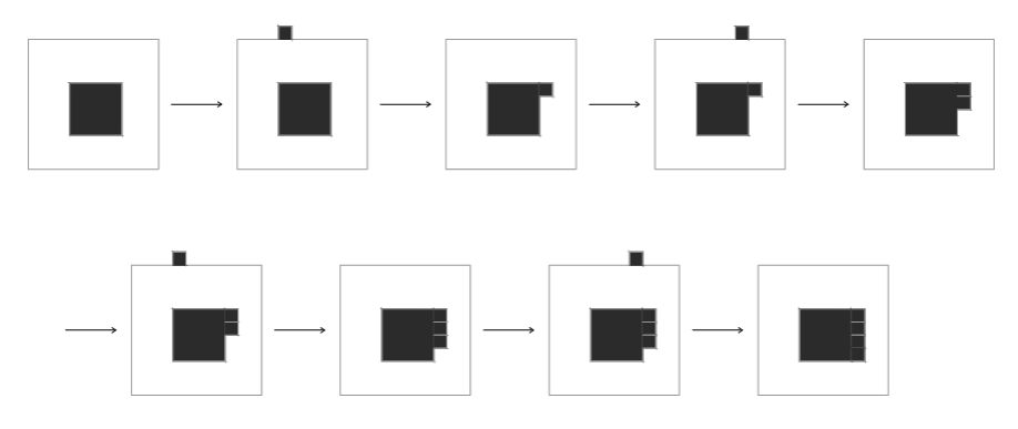
Figure 14: In the figure, the white part represents the region with zero spins, the dark gray region is the cluster of pluses. We observe that the configurations in this figure belongs to the path $\underline{\omega}$ but they are not communicating, indeed the free plus in the boundary must move in the box before to reach the cluster.

We construct a path in which at each step a particle of plus gets in $\Lambda$ and then it is attached to the cluster of pluses constructed before. We observe that every time that a particle gets in $\Lambda$ the energy cost is $\Delta^{p}$. The first two pluses get in $\Lambda$ and they possibly moves in the box until they are attached. When they are attached, a bond between plus spins is created and the energy decreases by $2J$. Then, another plus gets in $\Lambda$ and it moves towards the cluster of two particles. First the energy increases by $\Delta^{p}$ and then, when the plus reaches the cluster, it decreases by $2J$. The fourth plus get in $\Lambda$ with the same cost, but when it is attached to the cluster we obtain a square $2\times 2$ and two bonds between pluses are created, so the energy decreases by $4J$. Next, another two particles get in $\Lambda$ and they are attached clockwise to the square, so we obtain a quasi-square $2\times 3$ and so on. We note that when a particle is attached to the cluster the energy of the system decreases by at least $2J$. In particular, when we attach the first particle along a side of the quasi-square the energy decreases by $2J$, while the energy decreases by $4J$ when we attach the other particles along the same side. Next, we iterate this procedure by getting in $\Lambda$, moving and attaching a plus. In this way, we create squares and quasi-squares of pluses consequentially, until the cluster invades all the space $\Lambda_{0}$. In the following we compute the height of this path. First of all, we compute the energy of a configuration $\eta$ that contains a rectangle of pluses with side lengths $m$ and $n$ and only zero spins outside.

$$H(\eta)=H({\boldsymbol{0}})+2J(m+n)-(\lambda+h)mn$$ (4.83)

where $2(m+n)$ is the number of bonds $(0,+)$ and $mn$ is the number of pluses in $\eta$. The equation (4.83) attains the maximum in $(m,n)=\Big{(}\frac{2J}{\lambda+h},\frac{2J}{\lambda+h}\Big{)}$, that corresponds to a configuration with a square of pluses with side length $\tilde{n}=\lfloor\frac{2J}{\lambda+h}\rfloor+1$, called $\eta_{\tilde{n}}$. Starting from $\eta_{\tilde{n}}$ to reach the configuration $\eta_{\tilde{n}+1}$ that contains a quasi-square with side length $\tilde{n}$ and $\tilde{n}+1$, the energy cost is equal to $6J-2(\lambda+h)$ and it is given by the first three steps with a non-null energy cost. Indeed, this value is obtained by the sum between the positive cost $\Delta^{p}$ of the entrance of the first plus, the negative cost $-2J$ due to the junction of this plus to the cluster and the positive cost $\Delta^{p}$ of the entrance of the second plus $\Delta^{p}$. The rest of the path is a two-step downhill path indeed, a particle moves in $\Lambda$ by increasing the energy by $\Delta^{p}$ and then it is attached to the cluster by decreasing the energy by $4J>\Delta^{p}$, see Figure 14. Thus, recalling that $H({\boldsymbol{0}})=0$, using the value of $\tilde{n}$ and the assumption $2h>\lambda>h$, we have

$$\Phi({\boldsymbol{0}},{\boldsymbol{+1}})-H({\boldsymbol{0}})\leq\Phi(\eta_{\tilde{n}},\eta_{\tilde{n}+1})-H({\boldsymbol{0}})=H(\eta_{\tilde{n}})+6J-2(\lambda+h)-H({\boldsymbol{0}})$$

$$=4J\tilde{n}-(\lambda+h)\tilde{n}^{2}+6J-2(\lambda+h)=\frac{4J^{2}}{\lambda+h}+6J-2(\lambda+h)=V^{*}.$$ (4.84)

∎

5 Conclusions

We have studied the metastable behavior of the Blume–Capel model with magnetic field smaller than the chemical potential and we have been able to prove that, for this choice of the parameters, the minus homogeneous state is the unique metastable state. Moreover, we have studied in detail the transition from the metastable to the stable homogeneous plus state and we have provided an estimate of the exit time.

As we have explained above, see also the introductory section, the solution of the variational problems involved in the study of metastability is particularly difficult, because of the conservative nature of the Kawasaki dynamics and the interplay among the energy costs of different types of interfaces (the energy cost of the minus–plus lattice bonds is higher than that of the zero–plus and zero–minus ones).

The main problem is that, in order to minimize the energy cost of the interacting structure of pluses and minuses, it is necessary to separate them by means of a thin layer of zeros. Thus, the transition from the metastable minus state to the stable plus one must happen via the formation and growth of a droplet of pluses surrounded by a layer of zeros. This, associated with the swap character of the dynamics, is a huge problem, since, during the growth, it is not possible to create the necessary zeros and pluses where they are needed, but it is necessary to transport them from the boundary to these particular lattice sites through a completely arbitrary mixture of the three spin species.

We have solved this problem by introducing the idea of carpet, namely, a nearest neighbor connected set of lattice sites with constant spin value, and using these structures to transport spins along the lattice. The key lemma on which our study is based is Lemma 3.4 which allows us to control this transport mechanism and to estimate the involved energy costs.

For the sake of clearness, we have stated and proven this lemma in the context of the Blume–Capel model, but it is useful to remark that it is possible to state it in a more general setup, namely for multi–state spin systems. The generalized version of the lemma opens the way for the study of the metastable behavior of more general multi–state systems.

We thus wrap up this paper by stating the general version of the lemma. Let us, then, consider the generalized Potts model with spin variables taking value in $\{1,...,q\}$, with $q\in\mathbb{N}$. Given the lattice $\Lambda$ with periodic boundary conditions, the configuration space is $\mathcal{X}=\{1,...,q\}^{\Lambda}$ and the Hamiltonian function is given by

$$H(\sigma)=\sum_{\genfrac{}{}{0.0pt}{}{x,y\in\Lambda:}{|x-y|=1}}\!\!J(\sigma(x),\sigma(y))+\sum_{x\in\Lambda}h(\sigma(x)),$$ (5.85)

where $\sigma\in\mathcal{X}$ is a configuration, $J:\{1,\dots,q\}\times\{1,\dots,q\}\to\mathbb{R}$ gives the energy cost of the bond with spins $\sigma(x)$ and $\sigma(y)$, and $h:\{1,\dots,q\}\to\mathbb{R}$ is the magnetic field.

In the following we misuse the notation introduced in the paper for the Blume–Capel model and, mutatis mutandis, apply it to the generalized Potts model.

Lemma 5.15 (Weighted graph for the energy cost in $s$–carpet).

Let $s\in\{1,...,q\}$. Consider a configuration $\sigma\in\mathcal{X}$ such that there exists a $s$-carpet $X$ of $\sigma$ and two nearest neighboring sites $x\in\Lambda\setminus X$ and $x^{\prime}\in X$ such that $\sigma(x)=r\neq s$. Assume, also, that there exists $y\neq x^{\prime}$ a nearest neighbor of $x$ such that $\sigma(y)=s$. Let $X^{\prime}$ be the subset of $X$ obtained by collecting $x^{\prime}$ together with all the sites of $X$ having at least two neighboring sites in $X$. Then the following holds:

1. for any $v\in X^{\prime}\cup\{x\}$, let $\sigma^{v}=\sigma^{(x,v)}$ and recall $\sigma^{(x,x)}$ is equal to $\sigma$. Then, for any pair of neighboring sites $v,w\in X^{\prime}\cup\{x\}$

   $$H(\sigma^{v})-H(\sigma^{w})=[D_{v}(\sigma^{v})+D_{w}(\sigma^{v})]-[D_{v}(\sigma^{w})+D_{w}(\sigma^{w})]$$ (5.86)

   where

   $$D_{x}(\eta):=\left\{\begin{array}[]{cl}{\displaystyle\sum_{\begin{subarray}{c}y\in\Lambda:\\ |x-y|=1\end{subarray}}J(\eta(x),\eta(y))}&\textup{ if }x\in\Lambda_{0},\\ 0&\textup{ if }x\in\partial^{+}\Lambda_{0}.\end{array}\right.$$ (5.87)

2. For any $v\in X^{\prime}$

   $$\Phi(\sigma,\sigma^{v})-H(\sigma)\leq\max_{v\in X^{\prime}}\Big{(}[D_{v}(\sigma^{v})-D_{v}(\sigma)]+[D_{x}(\sigma^{v})-D_{x}(\sigma)]\Big{)}.$$ (5.88)

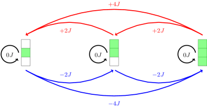
Figure 15: In each vertex of the graph the three squares represent three sites such that the one at the center is the site $x$ and it is nearest neighbor of the other two. The local configuration is reported with the colors green and white representing, respectively, the spin values $r$, and any other spin different from $r$. The other two sites neighboring the middle square and not reported in the picture are occupied by a fixed $s\neq r$ spin, indeed, in this example, we supposed that the configuration contains a $s$-carpet. The vertex at the center of the graph corresponds to any of the two reported configurations. Any transition from $\sigma^{v}$ to $\sigma^{w}$ for $v,w\in X^{\prime}\cup\{x\}$ is realized via the swap of the particle between two sites with local configuration represented by one of the vertices of the graph. For each possible swap the energy difference is reported in the picture.

In order to illustrate an interesting application of the Lemma 5.15 we consider the case of the ferromagnetic standard $q$–state Potts model and compute explicitely the energy difference $H(\sigma^{v})-H(\sigma^{w})$ and the communication height $\Phi(\sigma,\sigma^{v})-H(\sigma)$. In this case the interaction term is a negative constant for equal spins and zero otherwise, i.e.,

$$H(\sigma)=-J\sum_{\genfrac{}{}{0.0pt}{}{x,y\in\Lambda:}{|x-y|=1}}\!\!\textbf{1}_{\{\sigma(x)=\sigma(y)\}}+\sum_{x\in\Lambda}h(\sigma(x))$$ (5.89)

with $J>0$ and 1 is the characteristic function. Thus in this case, we have

$$H(\sigma^{v})-H(\sigma^{w})\in\{-4J,-2J,0,2J,4J\}\;\textup{ and }\;\Phi(\sigma,\sigma^{v})-H(\sigma)\leq 4J,$$ (5.90)

see Figure 15 for details.

Acknowledgements

ENMC thanks the Institute of Mathematics of the Utrecht University for the warm hospitality. ENMC thanks the PRIN 2022 project “Mathematical modelling of heterogeneous systems" (code 2022MKB7MM, CUP B53D23009360006). VJ thanks GNAMPA.

Data availability

Data sharing not applicable to this article as no datasets were generated or analysed during the current study.

Conflict of interest

The authors declare that they have no conflict of interest.

References

- [1] L. Alonso and R. Cerf. The three dimensional polyominoes of minimal area. the electronic journal of combinatorics, 3(1):R27, 1996.
- [2] V. Apollonio, V. Jacquier, F.R. Nardi, and A. Troiani. Metastability for the ising model on the hexagonal lattice. Electronic Journal of Probability, 27:1–48, 2022.
- [3] S. Baldassarri, A. Gallo, V. Jacquier, and A. Zocca. Ising model on clustered networks: A model for opinion dynamics. Physica A: Statistical Mechanics and its Applications, 623:128811, 2023.
- [4] S. Baldassarri and V. Jacquier. Metastability for kawasaki dynamics on the hexagonal lattice. Journal of Statistical Physics, 190(3):46, 2023.
- [5] S. Baldassarri and F.R. Nardi. Metastability in a lattice gas with strong anisotropic interactions under kawasaki dynamics. Electronic Journal of Probability, 26:1–66, 2021.
- [6] S. Baldassarri and F.R. Nardi. Critical droplets and sharp asymptotics for kawasaki dynamics with strongly anisotropic interactions. Journal of Statistical Physics, 186(3):34, 2022.
- [7] S. Baldassarri and F.R. Nardi. Critical droplets and sharp asymptotics for kawasaki dynamics with weakly anisotropic interactions. Stochastic Processes and their Applications, 147:107–144, 2022.
- [8] J. Beltrán and C. Landim. A martingale approach to metastability. Probability Theory and Related Fields, 161(1-2):267–307, 2015.
- [9] G. Bet, V. Jacquier, and F.R. Nardi. Effect of energy degeneracy on the transition time for a series of metastable states. Journal of Statistical Physics, 184:8, 2021.
- [10] M. Blume. Theory of the First–Order Magnetic Phase Change in UO2. Physical Review, 141:517, 1966.
- [11] A. Bovier and F. Den Hollander. Metastability: a potential-theoretic approach, volume 351. Springer, 2016.
- [12] A. Bovier, F. Den Hollander, and F.R. Nardi. Sharp asymptotics for Kawasaki dynamics on a finite box with open boundary. Probability theory and related fields, 135(2):265–310, 2006.
- [13] A. Bovier, F. Den Hollander, and C. Spitoni. Homogeneous nucleation for Glauber and Kawasaki dynamics in large volumes at low temperatures. The Annals of Probability, 38(2):661–713, 2010.
- [14] E.N.M. Cirillo, V. Jacquier, and C. Spitoni. Metastability of synchronous and asynchronous dynamics. Entropy, 24:450, 2022.
- [15] E.N.M. Cirillo, V. Jacquier, and C. Spitoni. Homogeneous and heterogeneous nucleation in the three-state blume–capel model. Physica D: Nonlinear Phenomena, 461:134125, 2024.
- [16] E.N.M. Cirillo and F.R. Nardi. Relaxation height in energy landscapes: an application to multiple metastable states. Journal of Statistical Physics, 150(6):1080–1114, 2013.
- [17] E.N.M. Cirillo, F.R. Nardi, and C. Spitoni. Sum of exit times in a series of two metastable states. The European Physical Journal Special Topics, 226(10):2421–2438, 2017.
- [18] E.N.M. Cirillo and E. Olivieri. Metastability and nucleation for the Blume-Capel model. different mechanisms of transition. Journal of Statistical Physics, 83(3-4):473–554, 1996.
- [19] T. Fiig, B.M. Gorman, P.A. Rikvold, and M.A. Novotny. Numerical transfer-matrix study of a model with competing metastable states. Physical Review E, 50:1930–1947, 1994.
- [20] A. Gaudillière, F. Den Hollander, F.R. Nardi, E. Olivieri, and E. Scoppola. Ideal gas approximation for a two-dimensional rarefied gas under Kawasaki dynamics. Stochastic Processes and their Applications, 119(3):737–774, 2009.
- [21] B. Gois and C. Landim. Zero-temperature limit of the kawasaki dynamics for the ising lattice gas in a large two-dimensional torus. Annals of Probability, 43:2151–2203, 2015.
- [22] F. Den Hollander, F.R. Nardi, E. Olivieri, and E. Scoppola. Droplet growth for three-dimensional Kawasaki dynamics. Probability theory and related fields, 125(2):153–194, 2003.
- [23] F. Den Hollander, F.R. Nardi, and A. Troiani. Metastability for low–temperature Kawasaki dynamics with two types of particles. Electronic Journ. of Probability, 17:1–26, 2012.
- [24] F. Den Hollander, E. Olivieri, and E. Scoppola. Metastability and nucleation for conservative dynamics. Journal of Mathematical Physics, 41(3):1424–1498, 2000.
- [25] H.W. Capel. On possibility of first–order phase transitions in ising systems of triplet ions with zero–field splitting. Physica, 32:966, 1966.
- [26] K. Kawsaki. Diffusion constants near the critical point for time–dependent ising models. Physical Review, 145:224–230, 1966.
- [27] C. Landim and P. Lemire. Metastability of the two–dimensional blume–capel model with zero chemical potential and small magnetic field. Journal of Statistical Physics, 164:346–376, 2016.
- [28] C. Landim, P. Lemire, and M. Mourragui. Metastability of the Two–Dimensional Blume–Capel Model with Zero Chemical Potential and Small Magnetic Field on a Large Torus. Journal of Statistical Physics, 175:456–494, 2019.
- [29] R. Lyons, E.N.M. Cirillo, and A. Muntean. Phase separation and morphology formation in interacting ternary mixtures under evaporation: Well-posedness and numerical simulation of a non-local evolution system. Nonlinear Analysis RWA, 77:104039, 2024.
- [30] R. Lyons, S.A. Muntean, E.N.M. Cirillo, and A. Muntean. A continuum model for morphology formation from interacting ternary mixtures: Simulation study of the formation and growth of patterns. Physica D, 453:133832, 2023.
- [31] F. Manzo, F.R. Nardi, E. Olivieri, and E. Scoppola. On the essential features of metastability: tunnelling time and critical configurations. Journal of Statistical Physics, 115(1-2):591–642, 2004.
- [32] F. Manzo and E. Olivieri. Dynamical Blume–Capel model: competing metastable states at infinite volume. Journal of Statistical Physics, 104(5-6):1029–1090, 2001.
- [33] S.A. Muntean, V.C.E. Kronberg, M. Colangeli, A. Muntean, J. van Stam, E. Moons, and E.N.M. Cirillo. Quantitative analysis of phase formation and growth in ternary mixtures upon evaporation of one component. Physical Review E, 106:025306, 2022.
- [34] F.R. Nardi, E. Olivieri, and E. Scoppola. Anisotropy effects in nucleation for conservative dynamics. Journal of Statistical Physics, 119(3-4):539–595, 2005.
- [35] E. Olivieri and M.E. Vares. Large deviations and metastability, volume 100. Cambridge University Press, 2005.