Integrated Sensing and Communication Enabled Cooperative Passive Sensing Using Mobile Communication System

Abstract

Integrated sensing and communication (ISAC) is a potential technology of the sixth-generation (6G) mobile communication system, which enables communication base station (BS) with sensing capability. However, the performance of single-BS sensing is limited, which can be overcome by multi-BS cooperative sensing. There are three types of multi-BS cooperative sensing, including cooperative active sensing, cooperative passive sensing, and cooperative active and passive sensing, where the multi-BS cooperative passive sensing has the advantages of low hardware modification cost and large sensing coverage. However, multi-BS cooperative passive sensing faces the challenges of synchronization offsets mitigation and sensing information fusion. To address these challenges, a non-line of sight (NLoS) and line of sight (LoS) signal cross-correlation (NLCC) method is proposed to mitigate carrier frequency offset (CFO) and time offset (TO). Besides, a symbol-level multi-BS sensing information fusion method is proposed. The discrete samplings of echo signals from multiple BSs are matched independently and coherent accumulated to improve sensing accuracy. Moreover, a low-complexity joint angle-of-arrival (AoA) and angle-of-departure (AoD) estimation method is proposed to reduce the computational complexity. Simulation results show that symbol-level multi-BS cooperative passive sensing scheme has an order of magnitude higher sensing accuracy than single-BS passive sensing. This work provides a reference for the research on multi-BS cooperative passive sensing.

I Introduction

TABLE I: Abbreviations and Notations

Abbreviation	Description	Abbreviation	Description
6G	Sixth-generation	2D	Two-dimensional
AoA	Angle-of-arrival	AoD	Angle-of-departure
AWGN	Additive white Gaussian noise	ADC	Analog-to-digital conversion
BS	Base station	CP	Cyclic prefix
CFO	Carrier frequency offset	CS	Compressed sensing
CACC	Cross-antenna cross-correlation	CASR	Cross-antenna signal ratio
CSI	Channel state information	DFT	Discrete Fourier transform
DAC	Digital-to-analog conversion	EVD	Eigenvalue decomposition
GPS	Global positioning system	IDFT	Inverse discrete Fourier transform
IoV	Internet of vehicle	ISAC	Integrated sensing and communication
LoS	Line of sight	MAP	Maximum a posteriori
MUSIC	Multiple signal classification	MIMO	Multi-Input Multi-Output
NLoS	Non-LoS	NLCC	NLoS and LoS signal cross-correlation
P/TBS	Passive/ Transmitting BS	RF	Radio frequency
Rx	Receiver	RMSE	Root mean square error
SNR	Signal-to-Noise ratio	Tx	Transmitter
TO	Time offset	ULA	Uniform linear array
Notation	Description	Notation	Description
${N_{\text{c}}}$	Number of subcarriers	$M_{\text{sym}}$	Number of OFDM symbols
$N_{\text{Tx}}^{i}$	Number of transmitting antenna in TBS	$N_{\text{Rx}}^{i}$	Number of receiving antenna in TBS
$N_{\text{Rx}}^{\text{p}}$	Number of receiving antenna in PBS	$n,n^{\prime}$	The index of subcarriers in frequency and time domain
$\mathbf{Y}_{\text{p},\text{ns}}^{i}$	the $i$-th all-antenna information matrix	$\phi_{\text{p},\text{ns}}^{i}$	AoA of the $i$-th TBS and PBS
$\theta_{i,\text{ns}}$	AoD of the $i$-th TBS and PBS	$\mathbf{D}_{\text{p},\text{ns}}^{i}$	The $i$-th delay-Doppler NLoS information matrix
$\mathbf{D}_{\text{p},\text{s}}^{i}$	The $i$-th delay-Doppler LoS information matrix	$\mathbf{D}_{\text{p}}^{i}$	The $i$-th delay-Doppler information matrix
$\mathbf{F}_{\text{p}}^{i},\mathbf{E}_{\text{p}}^{i}$	The $i$-th range and velocity feature vector	$\mathbf{P}_{\text{search}},\mathbf{V}_{\text{search}}$	The position and velocity searching scope matrix
$\mathbf{G}_{i}^{\text{mat}},\mathbf{S}_{i}^{\text{mat}}$	The $i$-th delay and Doppler matching matrix	$\mathbf{P}_{\text{fn}},\mathbf{V}_{\text{fn}}$	The final position and velocity profile
$\circ,\otimes$	The Hadamard and Kronecker product	$(\cdot)^{*}$	The conjugate operator
$(\cdot)^{\text{T}},(\cdot)^{\text{H}}$	The transpose and conjugate transpose operator	$v,\theta$	The magnitude and angle of the absolute velocity of target

The commonalities between wireless communication and radar sensing in terms of system design, hardware and frequency resources lay the foundations for integrated sensing and communication (ISAC) [1, 2, 3]. Recently, ISAC has become one of the key potential technologies of the sixth-generation (6G) mobile communication system [4, 5, 6, 7, 8]. The 6G mobile communication system is expected to facilitate the implementation of new applications, such as smart home, smart transportation and Internet of vehicles (IoV) [9, 10, 11]. These emerging applications urgently need high-accuracy sensing and high-capacity communication. Multi-BS cooperative sensing is a feasible method to provide high-accuracy sensing service [12, 13, 14].

According to the modes of sensing, multi-BS cooperative sensing can be categorized into multi-BS cooperative active sensing, multi-BS cooperative passive sensing, and multi-BS cooperative active and passive sensing [2]. Among the three types of cooperative sensing, multi-BS cooperative passive sensing has the following advantages.

1. Low hardware modification cost: The signal transmission process of passive sensing is similar to the communication process, which does not require the BS to transmit and receive signals simultaneously. Therefore, passive sensing can reuse the hardware equipment of communication system, greatly reducing the cost of hardware modification [15, 16].

2. Large sensing coverage: Passive sensing provides the advantage of continuous, all-encompassing reception of external radiation sources, eliminating the need for beam switching and beam scanning. Meanwhile, passive sensing offers a broader coverage of sensing compared with active sensing [17].

However, there are the following two main challenges in multi-BS cooperative passive sensing.

1. Synchronization offsets mitigation: Since the transmitter (Tx) and receiver (Rx) of passive sensing are separated, imperfect synchronization will cause time offsets (TOs) and carrier frequency offsets (CFOs), which further deteriorates the accuracy of range and velocity estimation [18].

2. Sensing information fusion: The current passive sensing information fusion methods seldom consider OFDM signal models, and it is difficult to achieve absolute velocity estimation of target.

The imperfect synchronization problem in cooperative passive sensing has been studied in radar sensing and WiFi sensing. In radar sensing, oscillator synchronization is usually aided by global positioning system (GPS). However, there are still synchronization errors in passive radar, which prevent further improvements in sensing accuracy. To this end, Younis et al. [19] proposed an alternate oscillator signal synchronization scheme that exchanges the oscillator signals by establishing a dedicated interstellar synchronization link to obtain the correction signal and compensate for it to achieve high-accuracy phase. However, exchanging oscillator signals may cause data acquisition interruptions. Jin et al. [20] adopted the time gap between the end of the echo reception window and the beginning of the next pulse repetition time to exchange the synchronization signals to further improve the synchronization accuracy. However, the performance of this method is affected by noise. In response, Cai et al. [21] exploited compressed sensing (CS) and maximum a posteriori (MAP) estimation to eliminate the noise in synchronization to achieve high synchronization accuracy. The above methods are specific to radar signals, and it is unclear whether they are applicable to communication signals. In terms of WiFi sensing, Zhang et al. summarized the methods to deal with clock desynchronization, including reference signal method, cross-antenna cross-correlation (CACC) method, and cross-antenna signal ratio (CASR) method [18]. The quality of the constructed reference signal significantly impacts the performance of the reference signal method. Qian et al. [22] used the CACC method to localization target with a single WiFi link for human tracking. However, this method is susceptible to the number of signal propagation paths. Therefore, Ni et al. [6] proposed an alternative scheme called mirrored multiple signal classification (MUSIC), which exploits the symmetry between the unknown parameters and reduces the computational complexity. However, the mirrored MUSIC method is limited by sensing range. To this end, based on the CASR principle, Zeng et al. [23] used the channel state information (CSI) ratio of two receiving antennas to obtain better sensing range and accuracy than CACC. The above CACC method amplifies noise and CASR method cannot be used for the signal fusion of cooperative passive sensing.

The other challenge in cooperative passive sensing is sensing information fusion. There are two main types of sensing information fusion methods in multi-BS cooperative passive sensing: data-level and symbol-level fusion. Data-level fusion is to fuse the information of target estimated by multiple nodes, thereby estimating the location and velocity of target. Weiss et al. [24] explored a method of gridding the possible locations of target, combining the delay estimation parameter of each node to estimate the location of target. However, the performance of this method is affected by grid size and noise. To minimize the impact of noise on the sensing accuracy, Ren et al. [25] presented a filtering and fusion method by evaluating the stability and consistency of sensing information of each node. However, this approach discards the sensing information of some nodes. In order to utilize the sensing information of all nodes, Jiang et al. [26] explored a weighted data fusion method for cooperative radar to obtain high-accuracy target position estimation by utilizing the optimal weight assignment. Data-level fusion is simple to implement but has limited sensing accuracy. Symbol-level fusion is to fuse the received sampling symbols from each node, which can overcome the limitation of data-level fusion. Oh et al. [27] proposed a decision-level (symbol-level) fusion method for intelligent vehicle systems, which achieves target-detection and classification. However, this method fails to achieve the velocity estimation of target. To this end, Gao et al. [28] implemented symbol-level fusion among neighboring radars to enhance sensing performance through strong signal correlation.

The symbol-level fusion improves the received signal-to-noise ratio (SNR) and obtains better sensing performance than data-level fusion. Therefore, this paper is dedicated to the symbol-level fusion approach. However, the symbol-level fusion methods in the above literature do not investigate the Doppler frequency shift of target in passive sensing as well as fully utilizing the geometric relationship between target and multiple BSs.

To address the above challenges, we propose a high-accuracy symbol-level multi-BS cooperative passive sensing scheme applicable to mobile communication systems. The detailed contributions are as follows.

• Symbol-level multi-BS cooperative passive sensing: For multi-BS cooperative target localization with symbol-level sensing information fusion, the searching scope is girded. Then, the feature vectors of target’s position are constructed and accumulated, further being applied to search the optimal estimation of target’s location from the grid points. This method achieves noise suppression and high-accuracy target localization. To estimate the absolute velocity of target, the searching scopes of angles and magnitudes of target’s velocity are girded. Then, an expression for the Doppler frequency shift due to the velocity of target is provided at the PBS. The velocity feature vectors are constructed and accumulated to realize the high-accuracy absolute velocity estimation of target.

• CFO and TO elimination method: For solving the synchronization problem between multiple BSs and avoiding ranging and velocity ambiguity, we propose a non-line of sight (NLoS) and line of sight (LoS) signal cross-correlation (NLCC) method on the passive BS (PBS) side. The signals on the LoS and NLoS paths between transmitting BS (TBS) and PBS are cross-correlated to eliminate the synchronization error. Simulation results demonstrate that this method mitigates CFO and TO in asynchronous multiple BSs.

• Joint AoA and AoD estimation method: A low-complexity, high-accuracy joint AoA and AoD estimation method is proposed to reduce the computational complexity of the AoA and AoD estimation, which achieves the same accuracy as the traditional two-dimensional MUSIC (2D-MUSIC) method while reducing the computational complexity.

The rest of this paper is organized as follows. Section II presents the ISAC signal model. In Section III, the data preprocessing in multi-BS passive sensing is proposed. In Section IV, the symbol-level fusion method in multi-BS passive sensing is studied, including the estimation methods of location and absolute velocity. In Section V, the performance analysis of radar sensing is revealed. In Section VI, the simulation results are shown. Section VII summarizes this paper. Table I shows the main variables and abbreviations in this paper.

II System Model

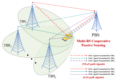
Figure 1: ISAC-enabled multi-BS cooperative passive sensing

II-A System Model

In this paper, we focus on the ISAC-enabled multi-BS cooperative passive sensing. As shown in Fig. 1, there are $I$ TBSs transmitting ISAC signals for passive sensing and downlink communication. PBS is receiving the downlink echo signal transmitted by TBSs from the LoS path and the NLoS paths, where the NLoS paths are produced by the signals transmitted from multiple TBSs. Without loss of generality, there are two assumptions in this paper [6, 18, 29, 30].

• Since TBSs are static, the PBS knows the locations of TBSs in advance. Then, the PBS can locate the absolute location of target through relative distance estimation.

• PBS knows the transmitted communication data of TBS in one of the following two ways: 1) TBS and PBS are connected by fiber optic cables, so that the PBS knows the transmitted data of TBS; 2) PBS could recognize and recover the communication data of TBS.

Meanwhile, each BS has a unique BS identity code to distinguish the signals of different BSs. Therefore, the signals from different TBSs can be distinguished at the PBS side [31].

II-B Signal Model

In this paper, we consider the BS with multiple input multiple output-orthogonal frequency division multiplying (MIMO-OFDM) and uniform linear array (ULA). For the $i\in\{1,2,\cdots,I\}$-th TBS, there are $N_{\text{Tx}}^{i}$ transmitting antennas and $N_{\text{Rx}}^{i}$ receiving antennas. For each PBS, there are $N_{\text{Rx}}^{\text{p}}$ receiving antennas.

II-B1 Transmit signal model

In the MIMO-OFDM system, a total number of $N_{\text{c}}$ subcarriers and $M_{\text{sym}}$ OFDM symbols are used for transmitting data. Therefore, the baseband transmit data matrix $\mathbf{X}$ in frequency domain can be expressed as [32]

$$\mathbf{X}=\left[\mathbf{X}_{1}^{\text{T}},\mathbf{X}_{2}^{\text{T}},\cdots,\mathbf{X}_{N_{\text{c}}}^{\text{T}}\right]^{\text{T}}\in\mathbb{C}^{N_{\text{c}}N_{\text{Tx}}^{i}\times M_{\text{sym}}},$$ (1)

where $\mathbf{X}_{n}\in\mathbb{C}^{N_{\text{Tx}}^{i}\times M_{\text{sym}}}$ denotes the baseband data matrix of the $n$-th subcarrier, and $n\in\left\{1,2,\cdots,N_{\text{c}}\right\}$ represents the index of subcarrier in frequency domain.

Then, the baseband transmit data (1) in frequency domain undergoes an $N_{\text{c}}$-point inverse discrete Fourier transform (IDFT) in time domain. Specifically, in the $i$-th TBS, the transmit modulation symbol of the $k$-th transmit antenna on the $n^{\prime}$-th subcarrier and the $m$-th OFDM symbol is [33]

$$x_{i}\left(k,m,n^{\prime}\right)=\frac{1}{N_{\text{c}}}\sum_{n=1}^{N_{\text{c}}}\mathbf{X}_{n}\left(k,m\right)e^{j2\pi n^{\prime}\frac{n}{N_{\text{c}}}},$$ (2)

where $\mathbf{X}_{n}\left(k,m\right)$ is the $\left(k,m\right)$-th element of $\mathbf{X}_{n}$, $m\in\left\{1,2,\cdots,M_{\text{sym}}\right\}$ denotes the index of OFDM symbols, $k\in\left\{1,2,\cdots,N_{\text{Tx}}^{i}\right\}$ denotes the antenna index of the $i$-th TBS, and $n^{\prime}\in\left\{1,2,\cdots,N_{\text{c}}\right\}$ denotes the subcarrier index in time domain.

To eliminate the inter-symbol interference (ISI) caused by frequency-selective fading, $N_{\text{cp}}$ points of cyclic prefix (CP) is inserted, which has a duration of $T_{\text{cp}}=\left(N_{\text{cp}}T_{\text{ofdm}}\right)/N_{\text{c}}$, where $T_{\text{ofdm}}$ denotes the duration of an OFDM symbol. Undergoing the digital-to-analog conversion (DAC) module, the baseband analog signal on the $k$-th transmitting antenna of the $i$-th TBS is expressed as [33]

$${\small\widetilde{x}(t)_{i}^{k}=\sum_{m=1}^{M_{\text{sym}}}\sum_{n^{\prime}=1}^{N_{\text{c}}}x_{i}\left(k,m,n^{\prime}\right)\text{rect}\left(t-\frac{n^{\prime}T}{N_{\text{c}}}-(m-1)T\right),}$$ (3)

where $T=T_{\text{ofdm}}+T_{\text{cp}}$ is total symbol duration, and $\text{rect}\left(\cdot\right)$ represents a rectangular window function with width $T$. Finally, the baseband analog signal is up-converted to the radio frequency (RF) domain via an RF link and transmitted by the antenna.

II-B2 Received signal model

According to Section II-A, there are LoS and NLoS paths between TBSs and PBS in multi-BS cooperative passive sensing. We assume that the real location of target is $\left(x^{\text{tar}},y^{\text{tar}}\right)$. In terms of NLoS path, the distance between the target and the PBS is $r_{\text{p,ns}}$, the distance between the target and the $i$-th TBS is $r_{i,\text{ns}}$, and the corresponding delays are $\tau_{\text{p,ns}}=r_{\text{p,ns}}/c$ and $\tau_{i,\text{ns}}=r_{i,\text{ns}}/c$, respectively. In terms of LoS path, since the location of each BS is known, the distance between the $i$-th TBS and PBS is known and is set to $r_{i,\text{s}}$. Then, we have $\tau_{i,\text{s}}=r_{i,\text{s}}/c$.

The error of synchronization between TBSs and PBS leads to potential time-varying TO and CFO [34], which are identical in both LoS and NLoS paths. The phase shift of the signal in NLoS path consists of CFO, TO, delay $\tau_{i,\text{p,ns}}=\tau_{i,\text{ns}}+\tau_{\text{p,ns}}$ and Doppler frequency shift $f_{i,\text{p}}$. $f_{i,\text{p}}$ is expressed as (4) by Theorem 1. The phase shift of the signal in LoS path includes path loss, delay, CFO, and TO.

Theorem 1

The target is located between TBS and PBS while traveling at an absolute velocity $\vec{v}$. When the space coordinate systems of BS and target are unified [13], the total Doppler frequency shift at PBS side is

$$f_{i,\text{p}}$$ (4)

$$=\frac{-vf_{\text{c}}}{c}{\left[\cos\left(\theta-\phi_{\text{p},\text{ns}}^{i}\right)+\cos\left(\theta-\theta_{i,\text{ns}}\right)\right]},\theta\in[0,2\pi),$$

where $v$ and $\theta$ are the magnitude and angle of target’s absolute velocity, respectively. $f_{\text{c}}$ and $c$ are the carrier frequency and speed of light, respectively.

Proof:

Assume that the angle of the velocity of target is along the counterclockwise rotation angle $\theta\in\left[0,2\pi\right)$, with a magnitude $v$. As shown in Fig. 2, the target is located between TBS and PBS, and the angle of the target’s velocity is arbitrary.

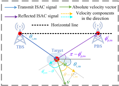
Figure 2: The locations of BSs and target

When the transmitted ISAC signal reaches the target, the movement of the target causes a Doppler frequency shift $f_{i,\text{p},1}=\frac{-vf_{\text{c}}\cos\left(\theta-\theta_{i,\text{ns}}\right)}{c}$ and the total carrier frequency is $f_{i,\text{p},2}=f_{\text{c}}+f_{i,\text{p},1}$. When the signal is reflected by the target and reaches the PBS, the reflected ISAC signal generates a Doppler frequency shift $f_{i,\text{p},3}$, which is

$$f_{{}_{i,\text{p},3}} =\frac{-v\cos\left(\theta-\phi_{\text{p},\text{ns}}^{i}\right)}{c}f_{i,\text{p},2}$$ (5)

$$=\frac{-vf_{\text{c}}\cos\left(\theta-\phi_{\text{p},\text{ns}}^{i}\right)}{c}$$

$$\quad+\frac{v^{2}f_{\text{c}}\cos\left(\theta-\phi_{\text{p},\text{ns}}^{i}\right)\cos\left(\theta-\theta_{i,\text{ns}}\right)}{c^{2}}.$$

It is worth noting that the carrier frequency is $f_{i,\text{p},2}$ instead of the original $f_{\text{c}}$. Therefore, the total Doppler frequency shift of the reflected echo ISAC signal received at PBS with respect to the transmitted ISAC signal at TBS is

$$f_{i,\text{p}} =f_{i,\text{p},1}+f_{i,\text{p},3}$$ (6)

$$=\frac{-vf_{\text{c}}\cos\left(\theta-\theta_{i,\text{ns}}\right)}{c}-\frac{vf_{\text{c}}\cos\left(\theta-\phi_{\text{p},\text{ns}}^{i}\right)}{c}$$

$$\quad+\frac{v^{2}f_{\text{c}}\cos\left(\theta-\phi_{\text{p},\text{ns}}^{i}\right)\cos\left(\theta-\theta_{i,\text{ns}}\right)}{c^{2}}.$$

As ${v^{2}}/{c^{2}}$ is very small, we ignore the quadratic term $\frac{v^{2}f_{\text{c}}\cos\left(\theta-\phi_{\text{p},\text{ns}}^{i}\right)\cos\left(\theta-\theta_{i,\text{ns}}\right)}{c^{2}}$ for simplicity, and (6) is transformed to

$$f_{i,\text{p}}=-\frac{vf_{\text{c}}}{c}{\left[\cos\left(\theta-\phi_{\text{p},\text{ns}}^{i}\right)+\cos\left(\theta-\theta_{i,\text{ns}}\right)\right]}.$$ (7)

∎

$$\mathbf{y}_{\text{p}}^{i}\left(m,n\right)\in\mathbb{C}^{N_{\text{Rx}}^{\text{p}}\times 1} =\mathbf{y}_{\text{p},\text{s}}^{i}\left(m,n\right)+\mathbf{y}_{\text{p},\text{s}}^{i}\left(m,n\right)$$ (8)

$$=\underbrace{b_{i,\text{p},\text{s}}e^{j2\pi mT\xi_{f,i}(m)}e^{-j2\pi n\Delta f\left[\tau_{i,\text{s}}+\xi_{\tau,i}(m)\right]}\mathbf{a}_{\text{Rx},\text{p}}\left(\theta_{i,\text{s}}\right)\mathbf{a}_{\text{Tx}}^{\text{T}}\left(\theta_{i,\text{s}}\right)\mathbf{x}_{m}^{i}}_{\text{LoS path}}$$

$$\quad+\underbrace{b_{i,\text{p},\text{ns}}e^{j2\pi mT\left[f_{i,\text{p}}+\xi_{f,i}\left(m\right)\right]}e^{-j2\pi n\Delta f\left[\tau_{i,\text{p},\text{ns}}+\xi_{\tau,i}\left(m\right)\right]}\mathbf{a}_{\text{Rx},\text{p}}\left(\phi_{\text{p},\text{ns}}^{i}\right)\mathbf{a}_{\text{Tx}}^{\text{T}}\left(\theta_{i,\text{ns}}\right)\mathbf{x}_{m}^{i}}_{\text{NLoS path}}+\mathbf{z}_{\text{S}}^{i}.$$

 

According to [35], for the PBS receiving the echo ISAC signal from the $i$-th TBS, the baseband received modulation symbol on the $n$-th subcarrier and the $m$-th OFDM symbol can be represented as (8), where $b_{i,\text{p,ns}}=\sqrt{\frac{\lambda^{2}}{\left(4\pi\right)^{3}r_{i,\text{ns}}^{2}r_{\text{p,ns}}^{2}}}\beta_{i,\text{p,ns}}$ and $b_{i,\text{p,s}}=\sqrt{\frac{\lambda^{2}}{\left(4\pi\right)^{3}r_{i,\text{s}}^{4}}}$ are the attenuations of LoS and NLoS paths, respectively. $\beta_{i,\text{p,ns}}$ is the reflecting factor of target. $\lambda=c/f_{\text{c}}$ is wavelength, $\Delta f=1/T_{\text{ofdm}}$ is subcarrier spacing. $\xi_{f,i}(m)$ and $\xi_{\tau,i}(m)$ are the CFO and TO of the $i$-th TBS, respectively. $\theta_{i,\text{s}}$ denotes the AoA and AoD of LoS path between the $i$-th TBS and PBS, which is known. $\mathbf{x}_{m}^{i}\in\mathbb{C}^{N_{\text{Tx}}^{i}\times 1}$ represents the data vector at the $m$-th OFDM symbol of $\mathbf{X}_{n}=\left[\mathbf{x}_{1}^{i},\mathbf{x}_{2}^{i},\cdots\mathbf{x}_{M_{\text{sym}}}^{i}\right]$. $\mathbf{z}_{\text{S}}^{i}\sim\mathcal{CN}\left(0,\sigma_{\text{S}}^{2}\right)$ is the AWGN of radar sensing channel. $\theta_{i,\text{ns}}$ and $\phi_{\text{p,ns}}^{i}$ denote the AoD of the signal from the $i$-th TBS to target and the AoA of the signal reflected from target arriving at the PBS, respectively. $\mathbf{a}_{\text{Rx},\text{p}}(\phi_{\text{p},\text{ns}}^{i})$ and $\mathbf{a}_{\text{Tx}}\left(\theta_{i,\text{ns}}\right)$ denote the receive steering vector of PBS and the transmit steering vector of the $i$-th TBS, respectively, as shown in (9).

$$\mathbf{a}_{\text{Rx},\text{p}}\left(\phi_{\text{p},\text{ns}}^{i}\right)=$$ (9)

$$\left[e^{j2\pi(\frac{d_{\text{r}}}{\lambda}){\sin(\phi_{\text{p},\text{ns}}^{i})}},e^{j4\pi(\frac{d_{\text{r}}}{\lambda}){\sin(\phi_{\text{p},\text{ns}}^{i})}},\cdots,e^{j\left(N_{\text{Rx}}^{\text{p}}\right){2\pi(\frac{d_{\text{r}}}{\lambda}){\sin(\phi_{\text{p},\text{ns}}^{i})}}}\right]^{\text{T}},$$

$$\mathbf{a}_{\text{Tx}}\left(\theta_{i,\text{ns}}\right)=$$

$$\left[e^{j{2\pi(\frac{d_{\text{r}}}{\lambda}){\sin(\theta_{i,\text{ns}})}}},e^{j{4\pi(\frac{d_{\text{r}}}{\lambda}){\sin(\theta_{i,\text{ns}})}}},\cdots,e^{j\left(N_{\text{Tx}}^{i}\right){2\pi(\frac{d_{\text{r}}}{\lambda}){\sin(\theta_{i,\text{ns}})}}}\right]^{\text{T}},$$

where $d_{\text{r}}$ is the distance between two adjacent antennas.

There are $I$ TBSs in multi-BS cooperative sensing. Hence, the echo signals received by PBS come from $I$ TBSs. Therefore, the echo modulation symbols received at PBS is

$$\mathbf{y}_{\text{p}}=\sum_{i=1}^{I}\sum_{m=1}^{M_{\text{sym}}}\sum_{n=1}^{N_{\text{c}}}\mathbf{y}_{\text{p}}^{i}(m,n).$$ (10)

The location and absolute velocity of target are obtained by processing and fusing the received data at PBS. Section III presents the preprocessing of the received data, including the estimation of AoA and AoD, the elimination of CFO and TO, and the data compression procedure, etc. Section IV investigates the data fusion and target sensing method.

III Multi-BS Signal Preprocessing

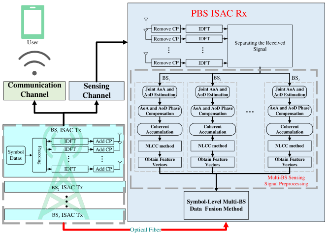
Figure 3: Multi-BS cooperative passive sensing scheme

As shown in Fig. 3, this section describes the preprocessing process of multi-BS signals. Specifically, we separate the received signals in PBS to obtain $I$ echo signals. For the $i$-th echo signal, we directly eliminate the AoA, AoD, and time delay of LoS path’s signal via phase compensation, followed by coherent accumulation and time-delay phase offset removal to obtain the delay-Doppler LoS information matrix $\mathbf{D}_{\text{p},\text{s}}^{i}$. For the NLoS path’s signal, we initially estimate AoA and AoD by the proposed low-complexity joint AoA and AoD estimation method. Subsequently, phase compensation aligns the phase of time-frequency signals over all antennas. Coherent accumulation enhances the SNR, generating the delay-Doppler NLoS information matrix $\mathbf{D}_{\text{p},\text{ns}}^{i}$.

CFO and TO in $\mathbf{D}_{\text{p},\text{ns}}^{i}$ will cause ambiguity in distance and velocity estimation [6]. To address this problem, a NLoS and LoS signal cross-correlation (NLCC) method is proposed for mitigating CFO and TO to generate the delay-Doppler information matrix $\mathbf{D}_{\text{p}}^{i}$. For $I$ delay-Doppler information matrices, we perform coherent compression processing to obtain range and velocity feature vectors (refer to Section III-D for details). Then, these feature vectors are utilized for symbol-level multi-BS sensing information fusion in Section IV.

III-A Low-complexity Joint AoA and AoD Estimation

The traditional 2D-MUSIC method for joint AoA-AoD estimation in MIMO-OFDM ISAC system generally has high computational complexity [36, 37]. Therefore, a two-step low-complexity joint AoA and AoD estimation method is proposed in this section.

For the $i$-th echo NLoS signal (e.g., the NLoS path in (8)), when the transmitted data vector $\mathbf{x}_{m}^{i}$ is known and the noise is not considered, right-multiplying the generalized inverse matrix $\left(\mathbf{x}_{m}^{i}\right)^{\text{H}}\left(\mathbf{x}_{m}^{i}\left(\mathbf{x}_{m}^{i}\right)^{\text{H}}\right)^{-1}$ on $\mathbf{y}_{\text{p},\text{ns}}^{i}(m,n)$ yields

$$\left(\mathbf{x}_{m}^{i}\right)^{\text{H}}\left(\mathbf{x}_{m}^{i}\left(\mathbf{x}_{m}^{i}\right)^{\text{H}}\right)^{-1}\mathbf{y}_{\text{p},\text{ns}}^{i}\big{(}m,n\big{)}$$ (11)

$$=b_{i,\text{p},\text{ns}}e^{j2\pi mT\left[f_{i,\text{p}}+\xi_{f,i}(m)\right]}e^{-j2\pi n\Delta f\left[\tau_{i,\text{p},\text{ns}}+\xi_{\tau,i}(m)\right]}$$

$$\quad\times\mathbf{a}_{\text{Rx},\text{p}}\left(J,\phi_{\text{p},\text{ns}}^{i}\right)\mathbf{a}_{\text{Tx}}^{\text{T}}\left(\theta_{i,\text{ns}}\right)\mathbf{I},$$

where $\mathbf{I}\in\mathbb{C}^{N_{\text{Tx}}^{{i}}\times N_{\text{Tx}}^{{i}}}$ is identity matrix, $\left(\cdot\right)^{\text{H}}$ is conjugate transpose operator, and an all-antenna information matrix is denoted by

$$\mathbf{Y}_{\text{p},\text{ns}}^{i}\in\mathbb{C}^{N_{\text{Rx}}^{\text{p}}\times N_{\text{Tx}}^{i}}=\left(\mathbf{x}_{m}^{i}\right)^{\text{H}}\left(\mathbf{x}_{m}^{i}\left(\mathbf{x}_{m}^{i}\right)^{\text{H}}\right)^{-1}\mathbf{y}_{\text{p},\text{ns}}^{i}\big{(}m,n\big{)}.$$ (12)

Observing (12), it is discovered that the AoA introduces a linear phase shift along the received antenna elements of $\mathbf{Y}_{\text{p},\text{ns}}^{i}$, while AoD introduces a linear phase shift along the transmit antenna elements of $\mathbf{Y}_{\text{p},\text{ns}}^{i}$. The most critical observation is that the phase shifts introduced by AoA and AoD are completely orthogonal.

III-A1 Rough estimation stage

In the rough estimation stage, we apply 2D-FFT method [38, 8] to obtain the rough estimation of AoA and AoD. Specifically, DFT is performed for each column and row of $\mathbf{Y}_{\text{p},\text{ns}}^{i}$ to obtain rough estimation of AoA and AoD, respectively. The above operation is expressed as [7]

$$\mathbf{Y}=\mathbf{F}_{N_{\text{Rx}}^{\text{p}}}\mathbf{Y}_{\text{p},\text{ns}}^{i}\mathbf{F}_{N_{\text{Tx}}^{i}}\in\mathbb{C}^{N_{\text{Rx}}^{\text{p}}\times{N_{\text{Tx}}^{i}}},$$ (13)

where $\mathbf{Y}$ denotes a 2D AoA-AoD profile and $\mathbf{F}_{N}\in\mathbb{C}^{N\times N}$ represents a DFT matrix. According to Theorem 2, we obtain the estimation results $\tilde{\phi}_{\text{p},\text{ns}}^{i}$ and $\tilde{\theta}_{i,\text{ns}}$, which narrow the searching range and reduce the computational complexity of 2D-MUSIC method. The updated search intervals are utilized for the fine estimation stage.

Theorem 2

When searching the peak value of $\mathbf{Y}$, the corresponding indices for the AoA-axis and AoD-axis are $\tilde{\mu}_{\phi}$ and $\tilde{\mu}_{\theta}$, respectively. Therefore, the rough estimation results of AoA and AoD are

$$\begin{cases}\begin{aligned} \tilde{\phi}_{\text{p},\text{ns}}^{i}&=\arcsin\left(\dfrac{\lambda\tilde{\mu}_{\phi}}{d_{\text{r}}N_{\text{Rx}}^{\text{p}}}\right),\\ \tilde{\theta}_{i,\text{ns}}&=\arcsin\left(\dfrac{\lambda\tilde{\mu}_{\theta}}{d_{\text{r}}N_{\text{Rx}}^{i}}\right),\end{aligned}\end{cases}$$ (14)

where $\arcsin\left({\cdot}\right)$ denotes the inverse sine function. Additionally, the resolution of rough estimation is

$$\begin{cases}\begin{aligned} \Delta\tilde{\phi}_{\text{p},\text{ns}}^{i}&=\arcsin\left(\dfrac{\lambda}{d_{\text{r}}N_{\text{Rx}}^{\text{p}}}\right),\\ \Delta\tilde{\theta}_{i,\text{ns}}&=\arcsin\left(\dfrac{\lambda}{d_{\text{r}}N_{\text{Rx}}^{i}}\right).\end{aligned}\end{cases}$$ (15)

Proof:

To perform the DFT on the rows and columns of $\mathbf{Y}_{\text{p}}^{i}$, the first row of $\mathbf{Y}_{\text{p}}^{i}$ is denoted by $\mathbf{r}_{1}\big{(}k,\theta_{i,\text{ns}}\big{)}$ and the first column of $\mathbf{Y}_{\text{p}}^{i}$ is denoted by $\mathbf{c}_{1}\big{(}J,\phi_{\text{p},\text{ns}}^{i}\big{)}$, where $J\in\{1,2,\cdots,N_{\text{Rx}}^{\text{p}}\}$ is the index of receiving antenna of PBS. Thus, the above operation is expressed as

$$\mathbf{C}_{1}\left(\mu_{\phi}\right)=\text{DFT}\left[\mathbf{c}_{1}\left(J,\phi_{\text{p},\text{ns}}^{i}\right)\right]$$ (16)

$$=\sum_{J=1}^{N_{\text{Rx}}^{\text{p}}}\mathbf{c}_{1}\left(J,\phi_{\text{p},\text{ns}}^{i}\right)e^{-j\frac{2\pi}{N_{\text{Rx}}^{\text{p}}}J\mu_{\phi}}$$

$$=\sum_{J=1}^{N_{\text{Rx}}^{\text{p}}}e^{j\frac{2\pi d_{\text{r}}}{\lambda}J\sin\left(\phi_{\text{p},\text{ns}}^{i}\right)}e^{-j\frac{2\pi}{N_{\text{Rx}}^{\text{p}}}J\mu_{\phi}},\mu_{\phi}=1,2,\cdots,N_{\text{Rx}}^{\text{p}},$$

and

$$\mathbf{R}_{1}\left(\mu_{\theta}\right)=\text{DFT}\left[\mathbf{r}_{1}\left(k,\theta_{i,\text{ns}}\right)\right]$$ (17)

$$=\sum_{k=1}^{N_{\text{Tx}}^{i}}\mathbf{r}_{1}\left(k,\theta_{i,\text{ns}}\right)e^{-j\frac{2\pi}{N_{\text{Tx}}^{i}}k\mu_{\theta}}$$

$$=\sum_{k=1}^{N_{\text{Tx}}^{i}}e^{jk\frac{2\pi d_{\text{r}}}{\lambda}\sin\left(\theta_{i,\text{ns}}\right)}e^{-j\frac{2\pi}{N_{\text{Tx}}^{i}}k{\mu_{\theta}}},\mu_{\theta}=1,2,\cdots,N_{\text{Tx}}^{{i}},$$

where $\mathbf{C}_{1}\left(\mu_{\phi}\right)$ and $\mathbf{R}_{1}\left(\mu_{\theta}\right)$ are AoA and AoD profiles, respectively. When searching for a peak, the corresponding AoA and AoD index values are

$$\tilde{\mu}_{\phi} =\left\lfloor\dfrac{N_{\text{Rx}}^{\text{p}}d_{\text{r}}\sin\left(\phi_{\text{p}}^{i}\right)}{\lambda}\right\rfloor,$$ (18)

$$\tilde{\mu}_{\theta} =\left\lfloor\frac{N_{\text{Tx}}^{i}d_{\text{r}}\sin\left(\theta_{i,\text{ns}}\right)}{\lambda}\right\rfloor,$$

where $\left\lfloor\cdot\right\rfloor$ represents floor function. Thus the rough estimations of AoA and AoD are obtained in (14). By observing (18), the index values of $\tilde{\mu}_{\phi}$ and $\tilde{\mu}_{\theta}$ only take integer values, whose resolution is $1$. The resolution of the corresponding rough estimation is shown in (15). ∎

III-A2 Fine estimation stage

In Section III-A1, the estimation results of $\tilde{\phi}_{\text{p},\text{ns}}^{i}$ and $\tilde{\theta}_{i,\text{ns}}$ are obtained via rough estimation. In this section, the fine estimation is performed. Specifically, we utilize $\tilde{\phi}_{\text{p},\text{ns}}^{i}$ and $\tilde{\theta}_{i,\text{ns}}$ to update the searching range of 2D-MUSIC method, reducing computational complexity and obtaining highly accurate estimation.

According to (18), only integers can be obtained in the rough estimation of $\tilde{\mu}_{\phi}$ and $\tilde{\mu}_{\theta}$. If the peak index values near the real AoA and AoD values are decimals, the real AoA and AoD values are around the estimated values in the rough estimation. Therefore, the searching range can be reduced to

$$\phi_{\text{search}}^{i}= \left[\arcsin\left(\frac{\lambda\left(\tilde{\mu}_{\phi}-1\right)}{d_{\text{r}}N_{\text{Rx}}^{\text{p}}}\right),\quad\arcsin\left(\frac{\lambda\left(\tilde{\mu}_{\phi}+1\right)}{d_{\text{r}}N_{\text{Rx}}^{\text{p}}}\right)\right],$$ (19)

$$\theta_{\text{search}}^{i}= \left[\arcsin\left(\frac{\lambda\left(\tilde{\mu}_{\theta}-1\right)}{d_{\text{r}}N_{\text{Rx}}^{i}}\right),\quad\arcsin\left(\frac{\lambda\left(\tilde{\mu}_{\theta}+1\right)}{d_{\text{r}}N_{\text{Rx}}^{i}}\right)\right].$$

For simplicity, (11) with noise can be expressed as

$$\mathbf{X}_{\text{p},\text{ns}}^{i}\left(m,n\right)$$ (20)

$$=\mathbf{a}_{\text{Rx},\text{p}}\left(\phi_{\text{p},\text{ns}}^{i}\right)\otimes\mathbf{a}_{\text{Tx}}\left(\theta_{i,\text{ns}}\right)\alpha(m,n)+\mathbf{n}(m,n),$$

where $\otimes$ represents the Kronecker product, $\alpha(m,n)$ denotes complex data, and $\mathbf{n}(m,n)$ is AWGN. Then, the 2D-MUSIC method [37] is applied with the updated searching ranges in fine estimation to obtain the final AoA estimation $\hat{\phi}_{\text{p},\text{ns}}^{i}$ and AoD estimation $\hat{\theta}_{i,\text{ns}}^{i}$. The 2D-MUSIC method is applied in this paper as follows.

• Step 1: The $i$-th transmitting signal in (20) is applied to obtain the covariance matrix $\hat{\mathbf{R}}_{\mathbf{y}_{\text{p},\text{ns}}^{i}}$.

  $$\hat{\mathbf{R}}_{\mathbf{y}_{\text{p},\text{ns}}^{i}}$$ (21)

  $$=\frac{1}{M_{\text{sym}}N_{\text{ c}}}\sum_{m=1}^{M_{\text{sym}}}\sum_{n=1}^{N_{\text{c}}}\mathbf{X}_{\text{p},\text{ns}}^{i}\left(m,n\right){\left[\mathbf{X}_{\text{p},\text{ns}}^{i}\left(m,n\right)\right]}^{\text{H}}.$$

• Step 2: The covariance matrix $\hat{\mathbf{R}}_{\mathbf{y}_{\text{p},\text{ns}}^{i}}$ undergoes an eigenvalue decomposition (EVD) to obtain [37]

  $$\operatorname{eig}\left(\hat{\mathbf{R}}_{\mathbf{y}_{\text{p},\text{ns}}^{i}}\right)=\mathbf{E}_{s}\mathbf{D}_{s}\mathbf{E}_{s}^{\text{H}}+\mathbf{E}_{n}\mathbf{D}_{n}\mathbf{E}_{n}^{\text{H}},$$ (22)

  where $\mathbf{D}_{s}$ and $\mathbf{D}_{n}$ denote the diagonal array of signal and noise, respectively, while $\mathbf{E}_{s}$ and $\mathbf{E}_{n}$ denote the sub-spaces of signal and noise, respectively.

• Step 3: Constructing the 2D-MUSIC spatial spectral functions $f_{\text{2d-music}}(\phi_{\text{s}},\theta_{\text{s}})$ [37]

  $$f_{{\text{2d-music}}}(\phi_{\text{s}},\theta_{\text{s}})$$ (23)

  $$=\frac{1}{\left[\mathbf{a}_{r}(\phi_{\text{s}})\otimes\mathbf{a}_{t}(\theta_{\text{s}})\right]^{\text{H}}\mathbf{E}_{n}\mathbf{E}_{n}^{\text{H}}\left[\mathbf{a}_{r}(\phi_{\text{s}})\otimes\mathbf{a}_{t}(\theta_{\text{s}})\right]},$$

  where

  $${\begin{gathered}\begin{aligned} &\mathbf{a}_{r}\left(\phi_{\text{s}}\right)=\\ &\left[\left.e^{j2\pi(\frac{d_{\text{r}}}{\lambda})\sin(\phi_{\text{s}})},e^{j4\pi(\frac{d_{\text{r}}}{\lambda})\sin(\phi_{\text{s}})},\cdots,e^{j\left(N_{\text{Rx}}^{\text{p}}\right)2\pi(\frac{d_{\text{r}}}{\lambda})\sin(\phi_{\text{s}})}\right]^{\text{T}},\right.\\ &\mathbf{a}_{t}\left(\theta_{\text{s}}\right)=\\ &\left[e^{j2\pi(\frac{d_{\text{r}}}{\lambda})\sin(\theta_{\text{s}})},e^{4\pi(\frac{d_{\text{r}}}{\lambda})\sin(\theta_{\text{s}})},\cdots,e^{j\left(N_{\text{Rx}}^{i}\right)2\pi(\frac{d_{\text{r}}}{\lambda})\sin(\theta_{\text{s}})}\right]^{\text{T}}.\end{aligned}\end{gathered}}$$ (24)

  $\phi_{\text{s}}$ and $\theta_{\text{s}}$ denote the searching values of AoA and AoD, respectively.

• Step 4: The peaks of $f_{\text{2d-music}}(\phi_{\text{s}},\theta_{\text{s}})$ are searched and the corresponding index values for the axes are the final estimation results of AoA and AoD .

Algorithm 1 provides a low-complexity joint AoA and AoD estimation method in Section III-A.

Algorithm 1: Low-complexity joint AoA and AoD estimation
Input:	All-antenna information matrix $\mathbf{Y}_{\text{p},\text{ns}}^{i}$; The number of OFDM symbols $M_{\text{sym}}$; The number of subcarriers $N_{\text{c}}$; The searching interval of 2D-MUSIC method $\varpi$.
Output:	The AoA and AoD estimation results $\hat{\phi}_{\text{p},\text{ns}}^{i}$ and $\hat{\theta}_{i,\text{ns}}$.
Rough estimation stage:
1:	Performing 2D-FFT on $\mathbf{Y}_{\text{p},\text{ns}}^{i}$, as shown in (13),
	the 2D AoA-AoD profile $\mathbf{Y}$ is obtained;
2:	for $\mathbf{Y}$ $\mu_{\phi}$ in $N_{\text{Rx}}^{\text{p}}$ and $\mu_{\theta}$ in $N_{\text{Tx}}^{i}$ do
3:	Get the maximum value of $\mathbf{Y}(\mu_{\phi},\mu_{\theta})$, denoted by $\mathbf{Y}(\tilde{\mu_{\phi}},\tilde{\mu_{\theta}})$;
4:	end for
5:	The AoA $\tilde{\phi}_{\text{p},\text{ns}}^{i}$ and AoD $\tilde{\theta}_{i,\text{ns}}$ are obtained via (14) and the peak indices $\tilde{\mu_{\phi}}$ and $\tilde{\mu_{\theta}}$ of the 2D AoA-AoD profile;
Fine estimation stage:
6:	The updated searching ranges are obtained via Eq. (19) and the peak indices $\tilde{\mu_{\phi}}$ and $\tilde{\mu_{\theta}}$ of the 2D AoA-AoD profile;
7:	The covariance matrix $\hat{\mathbf{R}}_{\mathbf{y}_{\text{p},\text{ns}}^{i}}$ is obtained by (21);
8:	The noise sub-space $\mathbf{E}_{n}$ is obtained by (22);
9:	for $\phi_{\text{s}},\theta_{\text{s}}$ in $\phi_{\text{search}}^{i},\theta_{\text{search}}^{i}$ with interval $\varpi$ do
10:	Spatial spectral functions $f_{\text{2d-music}}(\phi_{\text{s}},\theta_{\text{s}})$ are obtained     via noise sub-space and (23);
11:	The maximum value of $f_{\text{2d-music}}(\phi_{\text{s}},\theta_{\text{s}})$ is obtained;
12:	The corresponding AoA and AoD are obtained;
13:	end for
14:	The final AoA and AoD in fine estimation are obtained, denoted by $\hat{\phi}_{\text{p},\text{ns}}^{i}$ and $\hat{\theta}_{i,\text{ns}}$.

III-B Phase Compensation

In this subsection, the phase shifts in multiple antennas are compensated and coherent accumulation is performed to improve SNR. Specifically, the NLoS path signals and the LoS path signals are processed.

III-B1 NLoS path signals

When estimating the AoA $\hat{\phi}_{\text{p},\text{ns}}^{i}$ and the AoD $\hat{\theta}_{i,\text{ns}}$, the phase shifts caused by AoA and AoD of the NLoS signal in (8) can be eliminated. Without considering the noise component, the NLoS parts of the baseband received signal in the $J$-th receiving antenna on the $n$-th subcarrier and the $m$-th OFDM symbol time after compensation is

$$\mathbf{y}_{\text{p},\text{ns},\text{offset}}^{i}\left(J,m,n\right)=$$ (25)

$$\kappa_{i,\text{ns}}b_{i,\text{p},\text{ns}}e^{j2\pi mT\left[f_{i,\text{p}}+\xi_{f,i}(m)\right]}e^{-j2\pi n\Delta f\left[\tau_{i,\text{p},\text{ns}}+\xi_{\tau,i}(m)\right]},$$

where $J\in\{1,2,\cdots,N_{\text{Rx}}^{\text{p}}\}$ is the index of receive antenna on PBS and $\kappa_{i,\text{ns}}$ denotes the amplitude factor after the $i$-th NLoS path is compensated. According to (25), the signals on multi-antenna do not change with $J$ and have the same phase, which can be coherently accumulated to improve SNR. Therefore, the NLoS parts of the baseband received signal on the $n$-th subcarrier and the $m$-th OFDM symbol after coherent accumulation can be expressed as

$$\mathbf{y}_{\text{p},\text{ns},\text{offset},\text{coh}}^{i}\left(m,n\right)=\frac{1}{N_{\text{Rx}}^{\text{p}}}\sum_{J=1}^{N_{\text{Rx}}^{\text{p}}}\mathbf{y}_{\text{p},\text{ns},\text{offset}}^{i}\left(J,m,n\right).$$ (26)

The matrix form of (26) is shown in (27). $\mathbf{D}_{\text{p},\text{ns}}^{i}\in\mathbb{C}^{N_{\text{c}}\times M_{\text{sym}}}$ is referred to as delay-Doppler NLoS information matrix.

$$\centering\mathbf{D}_{\text{p},\text{ns}}^{i}=\left[\begin{array}[]{ccccc}\mathbf{y}_{\text{p},\text{ns},\text{offset},\text{coh}}^{i}\left(1,1\right)&\cdots&\mathbf{y}_{\text{p},\text{ns},\text{offset},\text{coh}}^{i}\left(1,m\right)&\cdots&\mathbf{y}_{\text{p},\text{ns},\text{offset},\text{coh}}^{i}\left(1,M_{\text{sym}}\right)\\ \vdots&\ddots&\vdots&\ddots&\vdots\\ \mathbf{y}_{\text{p},\text{ns},\text{offset},\text{coh}}^{i}\left(n,1\right)&\cdots&\mathbf{y}_{\text{p},\text{ns},\text{offset},\text{coh}}^{i}\left(n,m\right)&\cdots&\mathbf{y}_{\text{p},\text{ns},\text{offset},\text{coh}}^{i}\left(n,M_{\text{sym}}\right)\\ \vdots&\ddots&\vdots&\ddots&\vdots\\ \mathbf{y}_{\text{p},\text{ns},\text{offset},\text{coh}}^{i}\left(N_{\text{c}},1\right)&\cdots&\mathbf{y}_{\text{p},\text{ns},\text{offset},\text{coh}}^{i}\left(N_{\text{c}},m\right)&\cdots&\mathbf{y}_{\text{p},\text{ns},\text{offset},\text{coh}}^{i}\left(N_{\text{c}},M_{\text{sym}}\right)\\ \end{array}\right].\@add@centering$$ (27)

 

III-B2 LoS path signals

In the LoS path signals, AoA, AoD, and delay are known and can be directly eliminated, enabling coherent accumulation of the LoS path signals after removing these known parameters, including $\theta_{i,\text{s}}$ and $\tau_{i,\text{s}}$. Therefore, the LoS parts of the baseband received signal on the $n$-th subcarrier and the $m$-th OFDM symbol after coherent accumulation is expressed as

$$\mathbf{y}_{\text{p},\text{s},\text{offset}}^{i}\left(J,m,n\right)$$ (28)

$$=\kappa_{i,\text{s}}b_{i,\text{p},\text{s}}e^{j2\pi mT\xi_{f,i}(m)}e^{-j2\pi n\Delta f\xi_{\tau,i}(m)},$$

where $\kappa_{i,\text{s}}$ denotes the amplitude factor after the $i$-th LoS path is compensated. The result of the coherent accumulation of multi-antenna data in LoS path is referred to as the delay-Doppler LoS information matrix $\mathbf{D}_{\text{p},\text{s}}^{i}\in\mathbb{C}^{N_{\text{c}}\times M_{\text{sym}}}$.

III-C NLCC method

When $\mathbf{D}_{\text{p},\text{ns}}^{i}$ is utilized for the estimation of location and velocity of target, the CFO and TO lead to the ambiguity in distance and velocity estimation [6]. Therefore, NLCC method is proposed to mitigate the CFO and TO.

Observing $\mathbf{D}_{\text{p},\text{ns}}^{i}$ and $\mathbf{D}_{\text{p},\text{s}}^{i}$ obtained in Section III-B, the NLCC method is performed to mitigate the CFO and TO since both $\mathbf{D}_{\text{p},\text{ns}}^{i}$ and $\mathbf{D}_{\text{p},\text{s}}^{i}$ contain the same CFO and TO. With the cross-correlation on the corresponding elements of $\mathbf{D}_{\text{p},\text{ns}}^{i}$ and $\mathbf{D}_{\text{p},\text{s}}^{i}$, the delay-Doppler information matrix $\mathbf{D}_{\text{p}}^{i}\in\mathbb{C}^{N_{\text{c}}\times M_{\text{sym}}}$ is obtained, as shown in (29), where $\circ$ represents the Hadamard product and $(\cdot)^{*}$ is the conjugate operator.

$$\mathbf{D}_{\text{p}}^{i} =\mathbf{D}_{\text{p},\text{ns}}^{i}\circ\left(\mathbf{D}_{\text{p},\text{s}}^{i}\right)^{*}$$ (29)

$$=\kappa_{i,\text{s}}\kappa_{i,\text{ns}}b_{i,\text{p},\text{s}}b_{i,\text{p},\text{ns}}$$

$$\quad\times\left[\begin{array}[]{ccccc}e^{j2\pi Tf_{i,\text{p}}}e^{-j2\pi\Delta f\tau_{i,\text{p},\text{ns}}}&\cdots&e^{j2\pi mTf_{i,\text{p}}}e^{-j2\pi\Delta f\tau_{i,\text{p},\text{ns}}}&\cdots&e^{j2\pi M_{\text{sym}}Tf_{i,\text{p}}}e^{-j2\pi\Delta f\tau_{i,\text{p},\text{ns}}}\\ \vdots&\ddots&\vdots&\ddots&\vdots\\ e^{j2\pi Tf_{i,\text{p}}}e^{-j2\pi n\Delta f\tau_{i,\text{p},\text{ns}}}&\cdots&e^{j2\pi mTf_{i,\text{p}}}e^{-j2\pi n\Delta f\tau_{i,\text{p},\text{ns}}}&\cdots&e^{j2\pi M_{\text{sym}}Tf_{i,\text{p}}}e^{-j2\pi n\Delta f\tau_{i,\text{p},\text{ns}}}\\ \vdots&\ddots&\vdots&\ddots&\vdots\\ e^{j2\pi Tf_{i,\text{p}}}e^{-j2\pi N_{\text{c}}\Delta f\tau_{i,\text{p},\text{ns}}}&\cdots&e^{j2\pi mTf_{i,\text{p}}}e^{-j2\pi N_{\text{c}}\Delta f\tau_{i,\text{p},\text{ns}}}&\cdots&e^{j2\pi M_{\text{sym}}Tf_{i,\text{p}}}e^{-j2\pi N_{\text{c}}\Delta f\tau_{i,\text{p},\text{ns}}}\end{array}\right].$$

When CFO and TO are eliminated, the delay-Doppler information matrices undergo a coherent compression operation to reduce the data processing load while improving SNR. Section III-D describes the coherent compression operation in detail.

III-D Coherent Compression Operation

Observing $\mathbf{D}_{\text{p}}^{i}$, the initial phase of each row vector or each column vector is not aligned. The phase offset caused by delay remains constant across the elements within a subcarrier, while the Doppler effect maintains uniform phase shifts across the elements within an OFDM symbol. Therefore, a coherent compression operation is proposed for processing $\mathbf{D}_{\text{p}}^{i}$ to obtain the range feature vectors and velocity feature vectors, which can reduce the data processing load while improving SNR. The operational process unfolds as follows.

III-D1 Range feature vector

For $\mathbf{D}_{\text{p}}^{i}$, the $n$-th row vector of $\mathbf{D}_{\text{p}}^{i}$ is denoted by $\mathbf{F}_{\text{p}}^{i,n}$. To align the phase of each row vector, $\mathbf{F}_{\text{p}}^{i,1}$ is chosen as the reference row vector and the remaining $N_{\text{c}}-1$ row vectors are conjugated with $\mathbf{F}_{\text{p}}^{i,1}$ to obtain $N_{\text{c}}-1$ coherent row vectors. The $n^{\prime\prime}\in\left\{1,2,\cdots,N_{\text{c}}-1\right\}$-th coherent row vector is expressed as

$$\mathbf{F}_{\text{p},1}^{i,n^{\prime\prime}}\in\mathbb{C}^{1\times M_{\text{sym}}}=\mathbf{F}_{\text{p}}^{i,n^{\prime\prime}+1}\circ\left(\mathbf{F}_{\text{p}}^{i,1}\right)^{*}=$$ (30)

$$\left[e^{-j2\pi n^{\prime\prime}\Delta f\tau_{i,\text{p},\text{ns}}},e^{-j2\pi n^{\prime\prime}\Delta f\tau_{i,\text{p},\text{ns}}},\cdots,e^{-j2\pi n^{\prime\prime}\Delta f\tau_{i,\text{p},\text{ns}}}\right].$$

It is evident that by summing the elements in $\mathbf{F}_{\text{p},1}^{i,n^{\prime\prime}}$, SNR can be improved, as the elements are identical, while the accompanying noise remains random. Therefore, the elements in each of the $N_{\text{c}}-1$ coherent row vectors are summed to obtain the range feature vector $\mathbf{F}_{\text{p}}^{i}$, as shown in (31).

$$\mathbf{F}_{\text{p}}^{i}\in\mathbb{C}^{N_{\text{c}}-1\times 1}=\frac{1}{M_{\text{sym}}}\left[\sum_{m=1}^{M_{\text{sym}}}\mathbf{F}_{\text{p},1}^{i,1}(m),\cdots,\sum_{m=1}^{M_{\text{sym}}}\mathbf{F}_{\text{p},1}^{i,n^{\prime\prime}}(m),\cdots,\sum_{m=1}^{M_{\text{sym}}}\mathbf{F}_{\text{p},1}^{i,N_{\text{c}}-1}(m)\right]^{\text{T}}.$$ (31)

III-D2 Velocity feature vector

Similarly to the processing method of range feature vectors, the $m$-th column vector of $\mathbf{D}_{\text{p}}^{i}$ is denoted by $\mathbf{E}_{\text{p}}^{i,m}$. The $\mathbf{E}_{\text{p}}^{i,1}$ is chosen as the reference column vector and the remaining $M_{\text{sym}}-1$ column vectors are conjugated with $\mathbf{E}_{\text{p}}^{i,1}$ to obtain $M_{\text{sym}}-1$ coherent column vectors. The $m^{\prime}\in\left\{1,2,\cdots,M_{\text{sym}}-1\right\}$-th coherent column vector is

$$\mathbf{E}_{\text{p},1}^{i,m^{\prime}}\in\mathbb{C}^{N_{\text{c}}\times 1}=\mathbf{E}_{\text{p}}^{i,m^{\prime}+1}\circ\left(\mathbf{E}_{\text{p}}^{i,1}\right)^{*}$$ (32)

$$=\left[e^{j2\pi m^{\prime}Tf_{i,\text{p}}},e^{j2\pi m^{\prime}Tf_{i,\text{p}}},\cdots,e^{j2\pi m^{\prime}Tf_{i,\text{p}}}\right]^{\text{T}}.$$

Similarly, the elements of $\mathbf{E}_{\text{p},1}^{i,m^{\prime}}$ are identical. Therefore, we perform an operation similar to $\mathbf{F}_{\text{p},1}^{i,n^{\prime\prime}}$ to obtain the velocity feature vector $\mathbf{E}_{\text{p}}^{i}$, as shown in (33).

$$\mathbf{E}_{\text{p}}^{i}\in\mathbb{C}^{1\times M_{\text{sym}}-1}=\frac{1}{N_{\text{c}}}\left[\sum_{n=1}^{N_{\text{c}}}\mathbf{E}_{\text{p},1}^{i,1}(n),\cdots,\sum_{n=1}^{N_{\text{c}}}\mathbf{E}_{\text{p},1}^{i,m^{\prime}}(n),\cdots,\sum_{n=1}^{N_{\text{c}}}\mathbf{E}_{\text{p},1}^{i,M_{\text{sym}}-1}(n)\right].$$ (33)

 

The $I$ signals from TBSs are processed in Section III to obtain $I$ range feature vectors and $I$ velocity feature vectors, respectively. The above feature vectors are used to perform symbol-level multi-BS sensing information fusion.

IV Symbol-Level Multi-BS Sensing Information Fusion

In this section, a symbol-level multi-BS sensing information fusion method is proposed for cooperative passive sensing, including the location and absolute velocity estimation of target. Specifically, in the location estimation, the searching scope is first established. Given that the target is located in the overlapping coverage of multiple TBSs, whose location and coverage are known, the searching scope is calculated. Then, the searching scope is gridded to construct the position searching scope matrix (in (34)). Utilizing the position searching scope matrix, the distance vector (in (36)) associated with the $i$-th TBS is obtained. Subsequently, the distance compensation operation is performed, which value depends on the distance between the searching location and the PBS. The compensated distance vector (in (38)) is transformed into a delay matching matrix (in (39)) and is performed conjugate inner product with the corresponding $i$-th range feature vector, resulting in the $i$-th position profile (in (40)). The $I$ position profiles are coherent accumulated, and the index value corresponding to the peak value is the final location estimation of target. A similar process is carried out for velocity estimation. Fig. 4 shows the process of symbol-level multi-BS sensing information fusion method. A detailed description of the localization method and velocity estimation method is presented as follows.

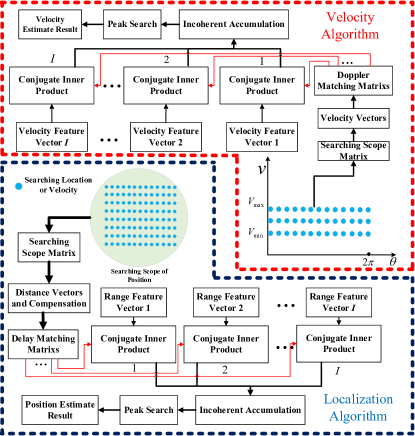
Figure 4: Flowchart of multi-BS data symbol-level fusion method

IV-A Localization Method

The localization method is given in detail in this subsection. In Section III, we obtain $I$ range and velocity feature vectors. Meanwhile, the searching scope of target is obtained. Then, the searching scope is girded to get the search interval matrix.

IV-A1 Obtain searching scope matrix

The searching scope of length and width $Q\Delta M$ is gridded with a step size $\Delta M$ to construct a position searching scope matrix $\mathbf{P}_{\text{search}}\in\mathbb{C}^{Q\times Q}$.

$$\mathbf{P}_{\text{search}}=$$ (34)

$$\left[\begin{array}[]{cccc}\left(x_{\text{ra},1},y_{\text{ra},1}\right)&\left(x_{\text{ra},1},y_{\text{ra},2}\right)&\cdots&\left(x_{\text{ra},1},y_{\text{ra},Q}\right)\\ \left(x_{\text{ra},2},y_{\text{ra},1}\right)&\left(x_{\text{ra},2},y_{\text{ra},2}\right)&\cdots&\left(x_{\text{ra},2},y_{\text{ra},Q}\right)\\ \vdots&\vdots&\ddots&\vdots\\ \left(x_{\text{ra},Q},y_{\text{ra},1}\right)&\left(x_{\text{ra},Q},y_{\text{ra},2}\right)&\cdots&\left(x_{\text{ra},Q},y_{\text{ra},Q}\right)\\ \end{array}\right],$$

where $\left(x_{\text{ra},p},y_{\text{ra},j}\right)$ indicates the coordinates within the searching scope with $p,j\in\left\{1,2,\cdots,Q\right\}$.

IV-A2 Obtain distance vectors and compensation

We assume that the coordinates of the $i$-th TBS are $\left(x^{i},y^{i}\right)$, while transforming $\mathbf{P}_{\text{search}}$ into row vector form to obtain the distance searching vector $\vec{\mathbf{P}}_{\text{search}}\in\mathbb{C}^{1\times Q^{2}}$.

$$\vec{\mathbf{P}}_{\text{search}}=\left[\text{vec}(\mathbf{P}_{\text{search}})\right]^{\text{T}},$$ (35)

where $\text{vec}(\cdot)$ represents the matrix vectorization. Then, the distance between each coordinate in $\vec{\mathbf{P}}_{\text{search}}$ and the location of the $i$-th TBS is calculated to obtain the $i$-th distance vector $\mathbf{G}_{\text{r}}^{i}\in\mathbb{C}^{1\times Q^{2}}$.

$$\mathbf{G}_{\text{r}}^{i}=\left[r_{i,1},r_{i,2},\cdots,r_{i,Q^{2}}\right],$$ (36)

where $r_{i,1}=\sqrt{\left(x^{i}-x_{\text{ra},1}\right)^{2}+\left(y^{i}-y_{\text{ra},1}\right)^{2}}$. However, $\mathbf{G}_{\text{r}}^{i}$ contains only the distance from the $i$-th TBS to the search location, which needs to be compensated for the distance from the search location to the PBS. Therefore, we calculate the distance between each coordinate in $\vec{\mathbf{P}}_{\text{search}}$ and the PBS to obtain the distance compensation vector $\mathbf{G}_{\text{cop}}\in\mathbb{C}^{1\times Q^{2}}$.

$$\mathbf{G}_{\text{cop}}=\left[r_{\text{p},1},r_{\text{p},2},\cdots,r_{\text{p},Q^{2}}\right].$$ (37)

Then, the $I$ vectors $\mathbf{G}_{\text{r}}^{i}$ are summed with $\mathbf{G}_{\text{cop}}$ to get $I$ compensated distance vectors, where the $i$-th compensated distance vector is

$$\mathbf{G}_{\text{r},i}^{\text{cop}}\in\mathbb{C}^{1\times Q^{2}}=\left[r_{1}^{\text{p},i},r_{2}^{\text{p},i},\cdots,r_{Q^{2}}^{\text{p},i}\right],$$ (38)

where $r_{p_{\text{d}}}^{\text{p},i}=r_{i,p_{\text{d}}}+r_{\text{p},p_{\text{d}}}$, $p_{\text{d}}\in\left\{1,2,\cdots,Q^{2}\right\}$.

IV-A3 Obtain distance matching matrices

According to the form of phase shifts generated by the delay along the frequency axis in [35], we transform the $I$ compensated distance vectors into delay matching matrices, where the $i$-th delay matching matrix $\mathbf{G}_{i}^{\text{mat}}\in\mathbb{C}^{N_{\text{c}}-1\times Q^{2}}$ is shown in (39).

$$\mathbf{G}_{i}^{\text{mat}}=\left[\begin{array}[]{ccccc}e^{-j2\pi\Delta f\left(\dfrac{r_{1}^{\text{p},i}}{c}\right)}&\cdots&e^{-j2\pi\Delta f\left(\dfrac{r_{p_{\text{d}}}^{\text{p},i}}{c}\right)}&\cdots&e^{-j2\pi\Delta f\left(\dfrac{r_{Q^{2}}^{\text{p},i}}{c}\right)}\\ \vdots&\ddots&\vdots&\ddots&\vdots\\ e^{-j2\pi n^{\prime\prime}\Delta f\left(\dfrac{r_{1}^{\text{p},i}}{c}\right)}&\cdots&e^{-j2\pi n^{\prime\prime}\Delta f\left(\dfrac{r_{p_{\text{d}}}^{\text{p},i}}{c}\right)}&\cdots&e^{-j2\pi n^{\prime\prime}\Delta f\left(\dfrac{r_{Q^{2}}^{\text{p},i}}{c}\right)}\\ \vdots&\ddots&\vdots&\ddots&\vdots\\ e^{-j2\pi\left(N_{\text{c}}-1\right)\Delta f\left(\dfrac{r_{1}^{\text{p},i}}{c}\right)}&\cdots&e^{-j2\pi\left(N_{\text{c}}-1\right)\Delta f\left(\dfrac{r_{p_{\text{d}}}^{\text{p},i}}{c}\right)}&\cdots&e^{-j2\pi\left(N_{\text{c}}-1\right)\Delta f\left(\dfrac{r_{Q^{2}}^{\text{p},i}}{c}\right)}\\ \end{array}\right].$$ (39)

 

IV-A4 Conjugate inner product

After processing in Sections IV-A1, IV-A2, and IV-A3, we obtain $I$ delay matching matrices $\mathbf{G}_{i}^{\text{mat}}$. In Section III, we obtain $I$ range feature vectors $\mathbf{F}_{\text{p}}^{i}$. In the following, we utilize $\mathbf{G}_{i}^{\text{mat}}$ and $\mathbf{F}_{\text{p}}^{i}$ to estimate the location of target.

The $i$-th $\mathbf{G}_{i}^{\text{mat}}$ and the corresponding $\mathbf{F}_{\text{p}}^{i}$ are performed conjugate inner product operation, which can be replaced by matrix multiplication. The $i$-th position profile $\mathbf{P}_{i}$ is shown in (40), where $\tau_{i,\text{p},p_{\text{d}}}=r_{p_{\text{d}}}^{\text{p},i}/c$. Then, a coherent accumulation operation is carried out to $I$ position profiles to obtain the final position profile $\mathbf{P}_{\text{fn}}$.

$$\mathbf{P}_{i}\in\mathbb{C}^{1\times Q^{2}}=\left(\mathbf{F}_{\text{p}}^{i}\right)^{\text{H}}\mathbf{G}_{i}^{\text{mat}}$$ (40)

$$=\left[\sum_{n^{\prime\prime}=1}^{N_{\text{c}}-1}e^{-j2\pi n^{\prime\prime}\Delta f\left(\tau_{i,\text{p},1}-\tau_{i,\text{p},\text{ns}}\right)},\sum_{n^{\prime\prime}=1}^{N_{\text{c}}-1}e^{-j2\pi n^{\prime\prime}\Delta f\left(\tau_{i,\text{p},2}-\tau_{i,\text{p},\text{ns}}\right)},\cdots,\sum_{n^{\prime\prime}=1}^{N_{\text{c}}-1}e^{-j2\pi n^{\prime\prime}\Delta f\left(\tau_{i,\text{p},Q^{2}}-\tau_{i,\text{p},\text{ns}}\right)}\right].$$

 

$$\mathbf{P}_{\text{fn}}=\frac{1}{I}\sum_{i=1}^{I}\mathbf{P}_{i},$$ (41)

the peak value of which is searched to obtain the peak index value $\tilde{p_{\text{d}}}$. The value of $\vec{\mathbf{P}}_{\text{search}}(\tilde{p_{\text{d}}})$ is the final estimated target location, denoted by $(\hat{x}_{\text{tar}},\hat{y}_{\text{tar}})$.

Algorithm 2 demonstrates the localization method in the symbol-level multi-BS sensing information fusion method.

Algorithm 2: Localization method
Input:	Range feature vectors $\mathbf{F}_{\text{p}}^{i},i\in\{1,2,\cdots,I\}$; The position searching scope of the target; The grid size $\Delta M$; The location of the $i$-th TBS $(x^{i},y^{i})$; The location of PBS $(x^{\text{p}},y^{\text{p}})$.
Output:	The estimated target location $(\hat{x}_{\text{tar}},\hat{y}_{\text{tar}})$.
Stage 1: The aim is to obtain distance matching matrices.
1:	Obtain the searching vector in (35) by
	the position searching scope and $\Delta M$;
2:	Obtain the distance compensation vector in (37) by
	the location of PBS $(x^{\text{p}},y^{\text{p}})$ and (35);
3:	for $i$ in $I$ do
4:	Obtain the $i$-th distance vectors in (36) by
	the location of PBS $(x^{i},y^{i})$ and (35);
5:	Obtain the $i$-th compensated distance vector in (38) by
	(36) and (37);
6:	Obtain the $i$-th delay matching matrix in (39) by (38);
7:	end for
Stage 2: The aim is to obtain the location of target.
8:	Initialize a final position profile $\mathbf{P}_{\text{fn}}$;
9:	for $i$ in $I$ do
10:	Obtain the $i$-th position profile in (40) by
	the $i$-th range feature vector $\mathbf{F}_{\text{p}}^{i}$ and (39);
11:	Storing the result in (40) in $\mathbf{P}_{\text{fn}}$;
12:	end for
13:	Obtain the final position profile $\mathbf{P}_{\text{fn}}$=$\mathbf{P}_{\text{fn}}$/$I$;
14:	Searching the peak of $\mathbf{P}_{\text{fn}}$ to obtain peak index $\tilde{p_{\text{d}}}$;
15:	Obtain the location of target $(\hat{x}_{\text{tar}},\hat{y}_{\text{tar}})$ by
	the peak index $\tilde{p_{\text{d}}}$ and (35);

IV-B Velocity Estimation Method

The velocity estimation method follows the same process as the localization method. The only difference is that no compensation is required because the derived Doppler frequency shift already includes the Doppler frequency shift from the TBS to target and from the target to PBS.

For the absolute velocity estimation of target, the scopes of the magnitude and angle of velocity are determined, denoted by $\left[V_{\text{min}},V_{\text{max}}\right]$ and $\left[0,2\pi\right]$, respectively. Then, the searching scope is gridded to obtain the velocity searching scope matrix, as shown in Fig. 4.

IV-B1 Obtain searching scope matrix

The searching scope of length $O\Delta\theta$ and width $S\Delta V$ is gridded with a step size of velocity’s magnitude $\Delta V$ and a step size of velocity’s direction $\Delta\theta$ to obtain a velocity searching scope matrix $\mathbf{V}_{\text{search}}\in\mathbb{C}^{S\times O}$.

$${\footnotesize\mathbf{V}_{\text{search}}=\left[\begin{array}[]{cccc}\left(v_{\text{ra},1},\theta_{\text{ra},1}\right)&\left(v_{\text{ra},1},\theta_{\text{ra},2}\right)&\cdots&\left(v_{\text{ra},1},\theta_{\text{ra},O}\right)\\ \left(v_{\text{ra},2},\theta_{\text{ra},1}\right)&\left(v_{\text{ra},2},\theta_{\text{ra},2}\right)&\cdots&\left(v_{\text{ra},2},\theta_{\text{ra},O}\right)\\ \vdots&\vdots&\ddots&\vdots\\ \left(v_{\text{ra},S},\theta_{\text{ra},1}\right)&\left(v_{\text{ra},S},\theta_{\text{ra},2}\right)&\cdots&\left(v_{\text{ra},S},\theta_{\text{ra},O}\right)\\ \end{array}\right],}$$ (42)

where $\left(v_{\text{ra},s},\theta_{\text{ra},o}\right)$ represents the searching magnitude and angle of velocity with $s\in\{1,2,\cdots,S\}$ and $o\in\{1,2,\cdots,O\}$.

IV-B2 Obtain velocity vectors and Doppler matrices

$\mathbf{V}_{\text{search}}$ is transformed into a column vector to obtain a velocity searching vector $\vec{\mathbf{V}}_{\text{search}}\in\mathbb{C}^{(S\times O)\times 1}$.

$$\vec{\mathbf{V}}_{\text{search}}=\text{vec}\left(\mathbf{V}_{\text{search}}\right).$$ (43)

Substituting the element from $\vec{\mathbf{V}}_{\text{search}}$, AoA $\hat{\phi}_{\text{p},\text{ns}}^{i}$ and AoD $\hat{\theta}_{i,\text{ns}}$ obtained in Section III-A, into (4) to obtain $I$ Doppler vectors, where the $i$-th Doppler vector is denoted as

$$\vec{\mathbf{S}}_{i}=\left[f_{i,\text{p}}^{1},f_{i,\text{p}}^{2},\cdots,f_{i,\text{p}}^{SO}\right]^{\text{T}},$$ (44)

where $f_{i,\text{p}}^{1}=\frac{-v_{\text{ra},1}f_{\text{c}}}{c}{\left[\cos\left(\theta_{\text{ra},1}-\hat{\phi}_{\text{p},\text{ns}}^{i}\right)+\cos\left(\theta_{\text{ra},1}-\hat{\theta}_{i,\text{ns}}\right)\right]}$.

According to the form of phase shifts generated by the Doppler frequency shift along the time axis in [35], the $I$ Doppler vectors are transformed into $I$ Doppler matching matrices, where the $i$-th Doppler matching matrix $\mathbf{S}_{i}^{\text{mat}}\in\mathbb{C}^{SO\times({M}_{\text{sym}}-1)}$ is expressed as

$$\mathbf{S}_{i}^{\text{mat}}=\left[\begin{array}[]{ccccc}e^{j2\pi Tf_{i,\text{p}}^{1}}&\cdots&e^{j2\pi m^{\prime}Tf_{i,\text{p}}^{1}}&\cdots&e^{j2\pi(M_{\text{sym}}-1)Tf_{i,\text{p}}^{1}}\\ \vdots&\vdots&\ddots&\vdots\\ e^{j2\pi Tf_{i,\text{p}}^{z}}&\cdots&e^{j2\pi m^{\prime}Tf_{i,\text{p}}^{z}}&\cdots&e^{j2\pi(M_{\text{sym}}-1)Tf_{i,\text{p}}^{z}}\\ \vdots&\vdots&\ddots&\vdots\\ e^{j2\pi Tf_{i,\text{p}}^{SO}}&\cdots&e^{j2\pi m^{\prime}Tf_{i,\text{p}}^{SO}}&\cdots&e^{j2\pi(M_{\text{sym}}-1)Tf_{i,\text{p}}^{SO}}\end{array}\right],$$ (45)

where $z\in\{1,2,\cdots,SO\}$.

IV-B3 Conjugate inner product

We obtain $I$ Doppler matching matrices in (45) and $I$ velocity feature vectors in (33). Then, they are utilized to estimate the absolute velocity of target.

For the $i$-th $\mathbf{S}_{i}^{\text{mat}}$ and the corresponding $\mathbf{E}_{\text{p}}^{i}$, the conjugate inner product operation is replaced by matrix multiplication. Then, the $i$-th velocity profile $\mathbf{V}_{i}$ after matrix multiplication is expressed in (46).

$$\mathbf{V}_{i}\in\mathbb{C}^{SO\times 1}=\mathbf{S}_{i}^{\text{mat}}\left(\mathbf{E}_{\text{p}}^{i}\right)^{\text{H}}$$ (46)

$$=\left[\sum_{m^{\prime}=1}^{M_{\text{sym}}-1}e^{j2\pi m^{\prime}T\left(f_{i,\text{p}}^{1}-f_{i,\text{p}}\right)},\sum_{m^{\prime}=1}^{M_{\text{sym}}-1}e^{j2\pi m^{\prime}T\left(f_{i,\text{p}}^{2}-f_{i,\text{p}}\right)},\cdots,\sum_{m^{\prime}=1}^{M_{\text{sym}}-1}e^{j2\pi m^{\prime}T\left(f_{i,\text{p}}^{SO}-f_{i,\text{p}}\right)}\right]^{\text{T}}.$$

 

Then, the $I$ velocity profiles are coherent accumulated to obtain the final velocity profile $\mathbf{V}_{\text{fn}}$.

$$\mathbf{V}_{\text{fn}}=\frac{1}{I}\sum_{i=1}^{I}\mathbf{V}_{i},$$ (47)

the peak value of which is searched to obtain the peak index value $\tilde{z}$. The value of $\vec{\mathbf{V}}_{\text{search}}(\tilde{z})$ is the final estimated target velocity, denoted by $(\hat{v},\hat{\theta})$.

Algorithm 3 demonstrates the velocity estimation method in the symbol-level multi-BS sensing information fusion method.

Algorithm 3: Velocity estimation method
Input:	Velocity feature vectors $\mathbf{E}_{\text{p}}^{i},i\in\{1,2,\cdots,I\}$; The velocity searching scope of the target; The grid size $\Delta\theta$ and $\Delta V$; The estimated AoA $\hat{\phi}_{\text{p},\text{ns}}^{i}$ and AoD $\hat{\theta}_{i,\text{ns}}$.
Output:	The estimated target velocity $(\hat{v},\hat{\theta})$.
Stage 1: The aim is to obtain velocity matching matrices.
1:	Obtain the searching vector in (43) by
	the velocity searching scope, the grid size $\Delta\theta$ and $\Delta V$;
2:	for $i$ in $I$ do
3:	Obtain the $i$-th Doppler vector in (44) by
	the estimated AoA $\hat{\phi}_{\text{p},\text{ns}}^{i}$, AoD $\hat{\theta}_{i,\text{ns}}$, and (4);
4:	Obtain the $i$-th Doppler matching matrix in (45) by
	(44);
5:	end for
Stage 2: The aim is to obtain the absolute velocity of target.
6:	Initialize a final velocity profile $\mathbf{V}_{\text{fn}}$;
7:	for $i$ in $I$ do
8:	Obtain the $i$-th velocity profile in (46) by
	the $i$-th velocity feature vector $\mathbf{E}_{\text{p}}^{i}$ and (45);
9:	Storing the result in (46) in $\mathbf{V}_{\text{fn}}$;
10:	end for
11:	Obtain the final velocity profile $\mathbf{V}_{\text{fn}}$=$\mathbf{V}_{\text{fn}}$/$I$;
12:	Searching the peak of $\mathbf{V}_{\text{fn}}$ to obtain peak index $\tilde{z}$;
13:	Obtain the absolute velocity of target $(\hat{v},\hat{\theta})$ by
	the peak index $\tilde{z}$ and (43) ;

V Performance Analysis of Multi-BS Cooperative Passive Sensing

In this section, the computational complexity of the joint AoA and AoD estimation method and the traditional 2D-MUSIC method, as well as the SNR in the symbol-level multi-BS sensing information fusion method, are analyzed.

V-A Complexity of Joint AoA and AoD Estimation Method

V-A1 Joint AoA and AoD estimation method

The computational complexity of 2D-MUSIC method for MIMO radar is derived in [37] as follows.

$$\mathcal{O}\{LM^{2}N^{2}+M^{3}N^{3}+\Theta^{2}[MN(MN-K)+MN-K]\},$$ (48)

where $K$ and $L$ denote the number of targets and snapshots, respectively; $M$ and $N$ denote the number of transmitting and receiving antennas, respectively; $\Theta$ denotes the total time spent in searching a dimension, where “dimension” refers to the searching scope for an unknown parameter. Inspired by (48), the computational complexity of the proposed method is derived as follows.

In the rough estimation stage, 2D-FFT is applied to estimate the AoA and AoD. The computational complexity of 2D-FFT is

$$\mathcal{O}\left\{N_{\text{Rx}}^{\text{p}}N_{\text{Tx}}^{i}\left[\left(N_{\text{Rx}}^{\text{p}}\right)^{2}+\left(N_{\text{Tx}}^{i}\right)^{2}\right]\right\}.$$ (49)

In the fine estimation stage, the searching scope is narrowed down as in (19). Then, the narrowed searching scope is gridded and the searching values are sequentially substituted into (23) to obtain the estimation of AoA and AoD. The grid sizes of AoA and AoD are expressed as follows.

$$\phi_{\text{step}}=\frac{\arcsin\left(\frac{\lambda\left(\tilde{\mu}_{\phi}+1\right)}{d_{\text{r}}N_{\text{Rx}}^{\text{p}}}\right)-\arcsin\left(\frac{\lambda\left(\tilde{\mu}_{\phi}-1\right)}{d_{\text{r}}N_{\text{Rx}}^{\text{p}}}\right)}{{\epsilon_{\phi}}},$$ (50)

$$\theta_{\text{step}}=\frac{\arcsin\left(\frac{\lambda\left(\tilde{\mu}_{\theta}+1\right)}{d_{\text{r}}N_{\text{Rx}}^{\text{bs}^{i}}}\right)-\arcsin\left(\frac{\lambda\left(\tilde{\mu}_{\theta}-1\right)}{d_{\text{r}}N_{\text{Rx}}^{\text{bs}^{i}}}\right)}{\epsilon_{\theta}},$$

where $\epsilon_{\phi}$ and $\epsilon_{\theta}$ denote the number of grids for the estimation of AoA and AoD, respectively. Meanwhile, the searching complexity of 2D-MUSIC is related to the number of grids in searching scope. Therefore, the searching complexity of 2D-MUSIC is $\mathcal{O}\{\epsilon_{\phi}\epsilon_{\theta}\}$ and the total computational complexity of the fine estimation stage is

$$\mathcal{O} \left\{M_{\text{sym}}N_{\text{c}}\left(N_{\text{Rx}}^{\text{p}}N_{\text{Tx}}^{i}\right)^{2}+\left(N_{\text{Rx}}^{\text{p}}N_{\text{Tx}}^{i}\right)^{3}\right.$$ (51)

$$\left.+\epsilon_{\phi}\epsilon_{\theta}\left[\left(N_{\text{Rx}}^{\text{p}}N_{\text{Tx}}^{i}+1\right)\left(N_{\text{Rx}}^{\text{p}}N_{\text{Tx}}^{i}-1\right)\right]\right\}.$$

Thus, the total computational complexity of the low-complexity joint AoA and AoD estimation method is shown in (52).

 

$$O\left\{\underbrace{N_{\text{Rx}}^{\text{p}}N_{\text{Tx}}^{i}\left[\left(N_{\text{Rx}}^{\text{p}}\right)^{2}+\left(N_{\text{Tx}}^{i}\right)^{2}\right]}_{\text{Rough stage}}+\underbrace{M_{\text{sym}}N_{\text{c}}\left(N_{\text{Rx}}^{\text{p}}N_{\text{Tx}}^{i}\right)^{2}+\left(N_{\text{Rx}}^{\text{p}}N_{\text{Tx}}^{i}\right)^{3}+\epsilon_{\phi}\epsilon_{\theta}\left[\left(N_{\text{Rx}}^{\text{p}}N_{\text{Tx}}^{i}+1\right)\left(N_{\text{Rx}}^{\text{p}}N_{\text{Tx}}^{i}-1\right)\right]}_{\text{Fine stage}}\right\}.$$ (52)

V-A2 Traditional 2D-MUSIC method

In deriving the computational complexity of the traditional 2D-MUSIC method, the grid sizes of the searching scope are set to $\phi_{\text{step}}$ and $\theta_{\text{step}}$ to ensure consistent estimation accuracy between traditional 2D-MUSIC method and proposed method. Meanwhile, the searching scope of both AoA and AoD are $\left(0,\ \pi\right]$, and the searching complexity of the traditional 2D-MUSIC is $\mathcal{O}\left\{\gamma_{\phi}\gamma_{\theta}\right\}$, where $\gamma_{\phi}=\pi/\phi_{\text{step}}$ and $\gamma_{\theta}=\pi/\theta_{\text{step}}$.

Therefore, the computational complexity of traditional 2D-MUSIC method is derived based on (48) as

$$\mathcal{O} \left\{\underbrace{M_{\text{sym}}N_{\text{c}}\left(N_{\text{Rx}}^{\text{p}}N_{\text{Tx}}^{{i}}\right)^{2}}_{(\text{a})}+\underbrace{\left(N_{\text{Rx}}^{\text{p}}N_{\text{Tx}}^{{i}}\right)^{3}}_{(\text{b})}\right.$$ (53)

$$\left.+\underbrace{\gamma_{\phi}\gamma_{\theta}\left[\left(N_{\text{Rx}}^{\text{p}}N_{\text{Tx}}^{{i}}+1\right)(N_{\text{Rx}}^{\text{p}}N_{\text{Tx}}^{{i}}-1)\right]}_{(\text{c})}\right\},$$

where (a) denotes the computational complexity of constructing covariance matrix, (b) denotes the computational complexity of eigenvalue decomposition [39], and (c) denotes the computational complexity of calculating and searching spatial spectral function.

V-B SNR of Symbol-Level Multi-BS Sensing Information Fusion Method

SNR is an important performance metric for sensing. In this section, the SNR gain of the proposed symbol-level multi-BS sensing information fusion method is derived.

Theorem 3

The SNR gain of the proposed symbol-level multi-BS sensing information fusion method is

$$\begin{cases}G_{\mathrm{P}}=\left(N_{\text{c}}-1\right)I\quad\left(\text{in location estimation}\right),\\ G_{\text{V}}=\left(M_{\text{sym}}-1\right)I\quad\left(\text{in velocity estimation}\right).\end{cases}$$ (54)

Proof:

Assuming that the modulus of the $n^{\prime\prime}$-th element of the $i$-th range feature vector $\mathbf{F}_{\text{p}}^{i}$ obtained in Section III is $h_{i}$ and the variance of the noise is $snr_{i}=h_{i}^{2}\sigma^{2}$, the SNR of $\mathbf{F}_{\text{p}}^{i}$ is $1/\sigma^{2}$. In the localization method, the operation in Sections IV-A1, IV-A2 and IV-A3 will not affect the SNR of $\mathbf{F}_{\text{p}}^{i}$. Therefore, the SNR gain originates solely from the operation of conjugate inner product.

Assume that the module of the $i$-th delay matching matrix $\mathbf{G}_{i}^{\text{mat}}$ is 1. For (40), the elements of the $i$-th position profile $\mathbf{P}_{i}$ are obtained by multiplying and summing each column of $\mathbf{G}_{i}^{\text{mat}}$ and $\mathbf{F}_{\text{p}}^{i}$ element by element. After the two elements are multiplied, as the module of $\mathbf{G}_{i}^{\text{mat}}$ is 1, the obtained result is the SNR of $\mathbf{F}_{\text{p}}^{i}$, which is $1/\sigma^{2}$. After the multiplication results are summed, the modules of signal and noise are $\left(N_{\text{c}}-1\right)h_{i}$ and $\left(N_{\text{c}}-1\right)h_{i}^{2}\sigma^{2}$, respectively. Therefore, the SNR of $\mathbf{P}_{i}$ is

$$snr_{\text{cm}}^{i}=\frac{\left(N_{\text{c}}-1\right)^{2}h_{i}^{2}}{\left(N_{\text{c}}-1\right)h_{i}^{2}\sigma^{2}}=\frac{\left(N_{\text{c}}-1\right)}{\sigma^{2}}.$$ (55)

(41) is a coherent accumulation operation. According to [40], the SNR gain of coherent accumulation is related to the number of summation terms. Therefore, the SNR of the final position profile $\mathbf{P}_{\text{fn}}$ is

$$snr_{\mathrm{f}}=\frac{\left(N_{\text{c}}-1\right)I}{\sigma^{2}},$$ (56)

and the SNR gain of the localization method is

$$G_{\text{P}}=\frac{snr_{\text{f}}}{snr_{i}}=\left(N_{\text{c}}-1\right)I.$$ (57)

Similarly, the SNR gain of the velocity estimation method is $G_{\text{V}}=\left(M_{\text{sym}}-1\right)I$. ∎

In summary, the proposed symbol-level multi-BS sensing information fusion method obtains the SNR gain compared with single-BS sensing, where the SNR gain is increasing with the increase of the number of TBSs.

TABLE II: Simulation parameters [38, 35, 1, 5]

Symbol	Parameter	Value	Symbol	Parameter	Value
$N_{\text{c}}$	Number of subcarriers	$512$	$M_{\text{sym}}$	Number of symbols	$256$
$f_{\text{c}}$	Carrier frequency	24 GHz	$\Delta f$	Subcarrier spacing	120 kHz
$T_{\text{ofdm}}$	Elementary NC-OFDM symbol duration	8.33 $\rm{\mu s}$	$T_{\text{p}}$	Cyclic prefix length	1.33 $\rm{\mu s}$
$T$	Entire NC-OFDM symbol duration	9.66 $\rm{\mu s}$	$I$	Number of TBS	$1\sim 4$
$N_{\text{Tx}}^{i}$	Number of transmitting antenna in TBS	$4$	$N_{\text{Rx}}^{\text{p}}$	Number of receiving antenna in TBS	$4$
$(x^{1},y^{1})$	The coordinate of the $1$-th TBS	(40 m, 0 m)	$(x^{2},y^{2})$	The coordinate of the $2$-th TBS	(0 m, 40 m)
$(x^{3},y^{3})$	The coordinate of the $3$-th TBS	(0 m, 80 m)	$(x^{4},y^{4})$	The coordinate of the $4$-th TBS	(80 m, 0 m)
$(x^{\text{p}},y^{\text{p}})$	The coordinate of PBS	(80 m, 80 m)	$(x^{\text{tar}},y^{\text{tar}})$	The coordinate of target	(40 m, 40 m)
$v$	Magnitude of velocity of the target	27 m/s	$\theta$	Angle of velocity of the target	0.785 radians
$\xi_{\tau,i}$	Value of TOs	$\left[30,60\right]$ ns	$\xi_{f,i}$	Value of CFOs	$\left[0.03,0.06\right]\ \Delta f$

VI Simulation

In this section, the proposed multi-BS cooperative passive sensing method is evaluated. Additionally, we compare the computational complexity of the proposed joint AoA and AoD estimation method with the traditional 2D-MUSIC method.

VI-A Multi-BS Cooperative Passive Sensing

In this section, the position and velocity profiles with symbol-level sensing information fusion method using three TBSs are simulated. Then, the root mean square errors (RMSEs) of location and velocity estimation are simulated. Table II shows the main simulation parameters, which satisfies the requirement of IoV [38, 35, 1, 5]. The simulation results are obtained with 10000 times Monte Carlo simulations.

VI-A1 Position profiles

To evaluate the feasibility of the proposed location estimation method, the simulation results are shown in Fig. 5 and the white lines represent contour lines.

Observing (a), (b), and (c) of Fig. 5, the trajectories of peak index values form a curve, which does not allow for accurate location estimation of target. Therefore, we can coherently accumulate multiple position profiles in (41) to obtain location estimation of target, resembling finding intersection point of multiple curves.

Fig. 5(d) shows the the final position profile obtained by performing coherent accumulation operation to the position profiles of three TBSs. According to (d) of Fig. 5, the location estimation of the target is (39.99 m, 39.99 m). The error of target location estimation in x-axis direction is 0.01 m, which reveals the feasibility of location estimation of the proposed multi-BS cooperative passive sensing method.

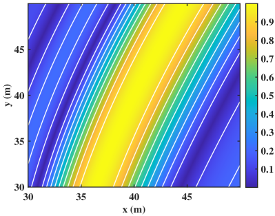
(a) Position profile of the 1-th TBS

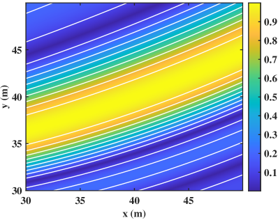
(b) Position profile of the 2-th TBS

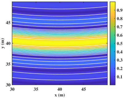
(c) Position profile of the 3-th TBS

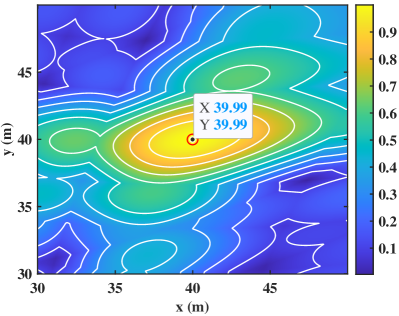
(d) The final position profile in (41)

Figure 5: Position profiles of location estimation with SNR = -5dB

VI-A2 Velocity profiles

To evaluate the feasibility of the proposed velocity estimation method, the simulation results are shown in Fig. 6.

The trajectories of peak index values in (a), (b), and (c) of Fig. 6 form a curve, which does not allow for accurate absolute velocity estimation of target. Therefore, we can coherently accumulate multiple velocity profiles in (47) to obtain the absolute velocity estimation of target, resembling finding intersection point of multiple curves.

As illustrated in (d) of Fig. 6, the peak corresponds to a velocity magnitude estimation of 27.3 m/s and an angle estimation of 0.754 radians. The errors in magnitude and angle estimation are 0.3 m/s and 0.03 radians, respectively, verifying the feasibility of absolute velocity estimation of the proposed multi-BS cooperative passive sensing method.

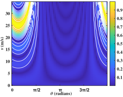
(a) Velocity profile of the 1-th TBS

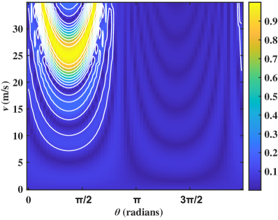
(b) Velocity of the 2-th TBS

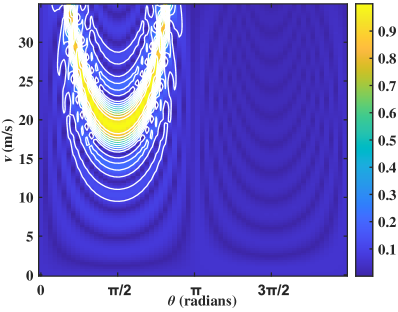
(c) Velocity of the 3-th TBS

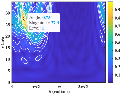
(d) The final velocity profile in (47)

Figure 6: Velocity profiles of velocity estimation with SNR = -5dB

VI-A3 RMSE of location estimation

The RMSE of location estimation with different numbers of TBSs are simulated as shown in Fig. 7. Observing the red, blue, and green lines in Fig. 7, when the SNR is higher than -10 dB, the accuracy of location estimation of target reaches the centimeter-level, revealing that the proposed multi-BS cooperative passive sensing scheme has high-accuracy location estimation of target. As the number of TBSs increases, the lines gradually decline, verifying the superiority of the proposed multi-BS cooperative passive sensing scheme compared with single-TBS passive sensing.

The performance of the proposed NLCC method is further simulated under different values of TOs, as shown in Fig. 8. Since the CFO has limited impact on the location estimation of target, a constant value is assigned when analyzing the performance of location estimation [41]. The solid and dashed lines refer to the cooperative passive sensing with and without NLCC, respectively. Cooperative passive sensing without NLCC refers to performing coherent compression directly using the delay-Doppler NLoS information matrices. The dotted line refers to the cooperative passive sensing without synchronization error.

Firstly, as the value of TO increases, the dashed lines rise, indicating that the impact of TO on the performance of location estimation is related to the value of TO. Secondly, the solid lines are lower and almost overlapped compared to the dashed lines, indicating that the proposed NLCC method can mitigate the degradation of location estimation performance caused by TO. Finally, the solid lines closely approximate the dotted line in high SNR region, indicating that the performance of NLCC method is improving with the increase of the SNR.

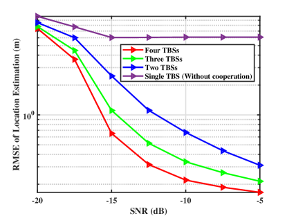
Figure 7: RMSE of location estimation for multi-BS cooperative passive sensing with TO = 30 ns and CFO = 0.03$\Delta f$

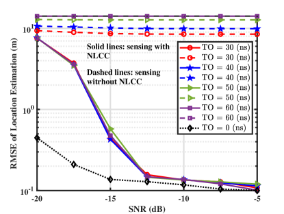
Figure 8: RMSE of location estimation with different TOs and CFO = 0.03$\Delta f$

VI-A4 RMSE of velocity estimation

The average RMSE of the magnitude and angle of velocity serves as the RMSE of velocity estimation in simulation. Absolute velocity estimation of target remains infeasible with single TBS passive sensing and is excluded from the simulation. Similarly, the RMSE of cooperative passive sensing with and without NLCC are compared. As shown in Figs. 9 and 10, the conclusions are similar to location estimation.

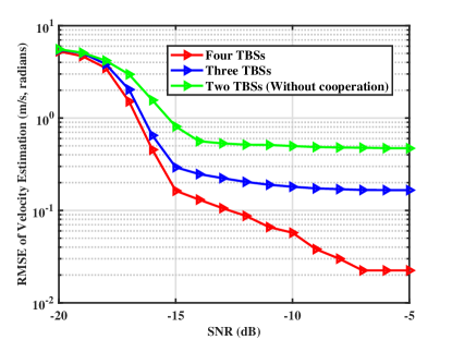
Figure 9: RMSE of velocity estimation for multi-BS cooperative passive sensing with TO = 30 ns and CFO = 0.03$\Delta f$

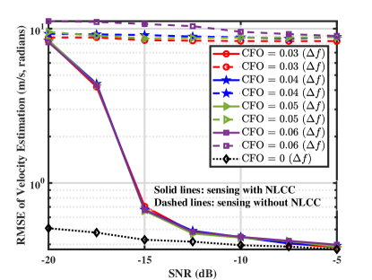
Figure 10: RMSE of velocity estimation with different CFOs and TO = 30 ns

VI-B Joint AoA and AoD Estimation

In this section, the computational complexity of the proposed joint AoA and AoD estimation method and traditional 2D-MUSIC method are simulated while ensuring the same estimation accuracy between the two methods. The estimation accuracy depends solely on the grid size of the fine estimation stage, thereby employing the same grid size $\phi_{\text{step}}$ = $\theta_{\text{step}}$ = 0.01 radians for both methods ensures the same estimation accuracy. The simulation results are revealed in Fig. 11, with the number of receiving antennas as the independent variable.

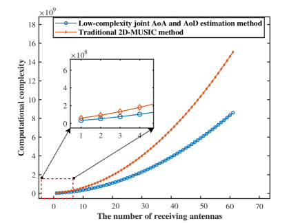
Figure 11: Computational complexity of the two methods

As shown in Fig. 11, the computational complexity of both methods increases rapidly with the increase of the number of receiving antennas. With the same number of receiving antennas, the computational complexity of the proposed method is lower than the traditional 2D-MUSIC method. Furthermore, the disparity in computational complexity between the two methods increases as the number of receiving antennas increases.

VII Conclusion

In this paper, a multi-BS cooperative passive sensing scheme is proposed to obtain high-accuracy sensing performance. To overcome the synchronization error in passive sensing, the NLCC method is proposed to mitigate the CFO and TO by correlating the sensing information in NLoS path and LoS path. Then, a symbol-level multi-BS sensing information fusion method is proposed to achieve high-accuracy location and absolute velocity estimation of target. Moreover, we propose a low-complexity joint AoA and AoD estimation method with rough and fine estimation stages to achieve high-accuracy AoA and AoD estimation with low complexity. The simulation results demonstrate the superiority of the proposed multi-BS cooperative passive sensing scheme, as well as the effectiveness of the proposed NLCC method.

References

• [1] Z. Wei, H. Liu, X. Yang, W. Jiang, H. Wu, X. Li, and Z. Feng, “Carrier aggregation enabled integrated sensing and communication signal design and processing,” IEEE Transactions on Vehicular Technology, Oct 2023.
• [2] Z. Wei, W. Jiang, Z. Feng, H. Wu, N. Zhang, K. Han, R. Xu, and P. Zhang, “Integrated Sensing and Communication enabled Multiple Base Stations Cooperative Sensing Towards 6G,” IEEE Network, Oct 2023.
• [3] H. Liu, Z. Wei, F. Li, Y. Lin, H. Qu, H. Wu, and Z. Feng, “ISAC Signal Processing Over Unlicensed Spectrum Bands,” arXiv preprint arXiv:2310.02555, 2023.
• [4] I. T. Union, “Future technology trends of terrestrial International Mobile Telecommunications systems towards 2030 and beyond,” 2022.
• [5] Z. Wei, R. Xu, Z. Feng, H. Wu, N. Zhang, W. Jiang, and X. Yang, “Symbol-level Integrated Sensing and Communication enabled Multiple Base Stations Cooperative Sensing,” IEEE Transactions on Vehicular Technology, Aug 2023.
• [6] Z. Ni, J. A. Zhang, X. Huang, K. Yang, and J. Yuan, “Uplink sensing in perceptive mobile networks with asynchronous transceivers,” IEEE Transactions on Signal Processing, vol. 69, pp. 1287–1300, Feb 2021.
• [7] F. Liu, Y. Cui, C. Masouros, J. Xu, T. X. Han, Y. C. Eldar, and S. Buzzi, “Integrated sensing and communications: Toward dual-functional wireless networks for 6G and beyond,” IEEE journal on selected areas in communications, vol. 40, no. 6, pp. 1728–1767, Mar 2022.
• [8] Z. Wei, H. Qu, Y. Wang, X. Yuan, H. Wu, Y. Du, K. Han, N. Zhang, and Z. Feng, “Integrated sensing and communication signals towards 5G-A and 6G: A survey,” IEEE Internet of Things Journal, Jan 2023.
• [9] Z. Xiao, R. Liu, M. Li, and Q. Liu, “A Novel Joint Angle-Range-Velocity Estimation Method for MIMO-OFDM ISAC Systems,” arXiv preprint arXiv:2308.03387, 2023.
• [10] X. Li, J. Zhang, C. Han, W. Hao, M. Zeng, Z. Zhu, and H. Wang, “Reliability and security of CR-STAR-RIS-NOMA assisted IoT networks,” IEEE Internet of Things Journal, Dec 2023.
• [11] X. Li, H. Qi, D.-T. Do, Z. Hui, Y. Ding, M. Zhu, and H. Peng, “IQ-Impaired Wireless-Powered Modify-and-Forward Relaying for IoT Networks: An In-Depth Physical Layer Security Analysis,” IEEE Internet of Things Journal, Feb 2023.
• [12] J. A. Zhang, M. L. Rahman, K. Wu, X. Huang, Y. J. Guo, S. Chen, and J. Yuan, “Enabling joint communication and radar sensing in mobile networks—A survey,” IEEE Communications Surveys & Tutorials, vol. 24, no. 1, pp. 306–345, Oct 2021.
• [13] W. Jiang, Z. Wei, B. Li, Z. Feng, and Z. Fang, “Improve Radar Sensing Performance of Multiple Roadside Units Cooperation via Space Registration,” IEEE Transactions on Vehicular Technology, vol. 71, no. 10, pp. 10 975–10 990, Oct. 2022.
• [14] Z. Wei, H. Qu, W. Jiang, K. Han, H. Wu, and Z. Feng, “Iterative Signal Processing for Integrated Sensing and Communication Systems,” IEEE Transactions on Green Communications and Networking, vol. 7, no. 1, pp. 401–412, Mar. 2023.
• [15] H. Kuschel, D. Cristallini, and K. E. Olsen, “Tutorial: Passive radar tutorial,” IEEE Aerospace and Electronic Systems Magazine, vol. 34, no. 2, pp. 2–19, Feb 2019.
• [16] X. Li, J. Li, Y. Liu, Z. Ding, and A. Nallanathan, “Residual transceiver hardware impairments on cooperative NOMA networks,” IEEE Transactions on Wireless Communications, vol. 19, no. 1, pp. 680–695, Oct 2019.
• [17] W. Xianrong, Y. Jianxin, Z. Weijie, X. Deqiang, S. Kan, S. Jiale, C. Feng, R. Yunhua, G. Ziping, and K. Hengyu, “Research progress and development trend of the multi-illuminator-based passive radar,” Journal of Radars, vol. 9, no. 6, pp. 939–958, Dec 2020.
• [18] J. A. Zhang, K. Wu, X. Huang, Y. J. Guo, D. Zhang, and R. W. Heath, “Integration of radar sensing into communications with asynchronous transceivers,” IEEE Communications Magazine, vol. 60, no. 11, pp. 106–112, Aug 2022.
• [19] M. Younis, R. Metzig, and G. Krieger, “Performance prediction of a phase synchronization link for bistatic sar,” IEEE Geoscience and Remote Sensing Letters, vol. 3, no. 3, pp. 429–433, Jul 2006.
• [20] G. Jin, K. Liu, D. Liu, D. Liang, H. Zhang, N. Ou, Y. Zhang, Y. Deng, C. Li, and R. Wang, “An advanced phase synchronization scheme for LT-1,” IEEE Transactions on Geoscience and Remote Sensing, vol. 58, no. 3, pp. 1735–1746, Nov 2019.
• [21] Y. Cai, R. Wang, W. Yu, D. Liang, K. Liu, H. Zhang, and Y. Chen, “An advanced approach to improve synchronization phase accuracy with compressive sensing for LT-1 bistatic spaceborne SAR,” Remote Sensing, vol. 14, no. 18, p. 4621, Sep 2022.
• [22] K. Qian, C. Wu, Y. Zhang, G. Zhang, Z. Yang, and Y. Liu, “Widar2. 0: Passive human tracking with a single Wi-Fi link,” in Proceedings of the 16th annual international conference on mobile systems, applications, and services, Jun 2018, pp. 350–361.
• [23] Y. Zeng, D. Wu, J. Xiong, E. Yi, R. Gao, and D. Zhang, “FarSense: Pushing the range limit of WiFi-based respiration sensing with CSI ratio of two antennas,” Proceedings of the ACM on Interactive, Mobile, Wearable and Ubiquitous Technologies, vol. 3, no. 3, pp. 1–26, Sep 2019.
• [24] A. J. Weiss and A. Amar, “Direct geolocation of stationary wideband radio signal based on time delays and Doppler shifts,” in 2009 IEEE/SP 15th Workshop on Statistical Signal Processing.   IEEE, Oct 2009, pp. 101–104.
• [25] M. Ren, P. He, and J. Zhou, “Improved Shape-Based Distance Method for Correlation Analysis of Multi-Radar Data Fusion in Self-Driving Vehicle,” IEEE Sensors Journal, vol. 21, no. 21, pp. 24 771–24 781, Sep 2021.
• [26] W. Jiang, Z. Qi, Z. Ye, Y. Wan, and L. Li, “Research on Cooperative Detection Technology of Networked Radar Based on Data Fusion,” in 2021 2nd China International SAR Symposium (CISS).   IEEE, Dec 2021, pp. 1–5.
• [27] S.-I. Oh and H.-B. Kang, “Object detection and classification by decision-level fusion for intelligent vehicle systems,” Sensors, vol. 17, no. 1, p. 207, Jan 2017.
• [28] B. Gao, M. Jia, T. Zhang, and Q. Zhang, “Reliable target positioning in complicated environments using multiple radar observations,” in 2021 IEEE Global Communications Conference (GLOBECOM).   IEEE, Feb 2021, pp. 1–6.
• [29] S. Venkatesh and R. Buehrer, “Non-line-of-sight identification in ultra-wideband systems based on received signal statistics,” IET Microwaves, Antennas & Propagation, vol. 1, no. 6, pp. 1120–1130, Dec 2007.
• [30] Z. Wang, W. Xu, and S. A. Zekavat, “A new multi-antenna based los-nlos separation technique,” in 2009 IEEE 13th Digital Signal Processing Workshop and 5th IEEE Signal Processing Education Workshop.   IEEE, Feb 2009, pp. 331–336.
• [31] A. Chouchane, S. Rekhis, and N. Boudriga, “Defending against rogue base station attacks using wavelet based fingerprinting,” in 2009 IEEE/ACS International Conference on Computer Systems and Applications.   IEEE, Jun 2009, pp. 523–530.
• [32] X. Hu, C. Masouros, F. Liu, and R. Nissel, “Low-PAPR DFRC MIMO-OFDM Waveform Design for Integrated Sensing and Communications,” in ICC 2022-IEEE International Conference on Communications.   IEEE, Aug 2022, pp. 1599–1604.
• [33] P. Aggarwal and V. A. Bohara, “Characterization of HPA using two dimensional general memory polynomial for dual band carrier aggregated MIMO-OFDM systems,” in 2016 IEEE International Conference on Communications (ICC).   IEEE, Jul 2016, pp. 1–7.
• [34] K. Wu, J. A. Zhang, and Y. J. Guo, Joint communications and sensing: From fundamentals to advanced techniques.   John Wiley & Sons, Dec 2022.
• [35] C. Sturm and W. Wiesbeck, “Waveform design and signal processing aspects for fusion of wireless communications and radar sensing,” Proceedings of the IEEE, vol. 99, no. 7, pp. 1236–1259, May 2011.
• [36] I. Pasya, N. Iwakiri, and T. Kobayashi, “Joint direction-of-departure and direction-of-arrival estimation in an ultra-wideband MIMO radar system,” in 2014 IEEE Radio and Wireless Symposium (RWS).   IEEE, Jun 2014, pp. 52–54.
• [37] X. Zhang, L. Xu, L. Xu, and D. Xu, “Direction of departure (DOD) and direction of arrival (DOA) estimation in MIMO radar with reduced-dimension MUSIC,” IEEE communications letters, vol. 14, no. 12, pp. 1161–1163, Nov 2010.
• [38] C. Sturm, T. Zwick, and W. Wiesbeck, “An OFDM system concept for joint radar and communications operations,” in VTC Spring 2009-IEEE 69th Vehicular Technology Conference.   IEEE, Jun 2009, pp. 1–5.
• [39] L. N. Trefethen and D. Bau, Numerical linear algebra.   Siam, Jun 2022, vol. 181.
• [40] M. A. Richards, “Noncoherent integration gain, and its approximation,” Georgia Institute of Technology, Technical Memo, Jun 2010.
• [41] W. Jiang, Z. Wei, S. Yang, Z. Feng, and P. Zhang, “Cooperation Based Joint Active and Passive Sensing with Asynchronous Transceivers for Perceptive Mobile Networks,” arXiv preprint arXiv:2312.02163, 2023.