An indirect geometry crystal time-of-flight spectrometer for FRM II

Abstract

We present a concept for an indirect geometry crystal time-of-flight spectrometer, which we propose for the FRM-II reactor in Garching. Recently, crystal analyzer spectrometers at modern spallation sources have been proposed and are under construction. The secondary spectrometers of these instruments are evolutions of the flat cone multi-analyzer for three-axis spectrometers (TAS). The instruments will provide exceptional reciprocal space coverage and intensity to map out the excitation landscape in novel materials. We will discuss the benefits of such a time-of-flight primary spectrometer with a large crystal analyzer spectrometer at a continuous neutron source. The dynamical range can be very flexibly matched to the requirements of the experiment without sacrificing the neutron intensity. At the same time, the chopper system allows a quasi-continuous variation of the initial energy resolution. The neutron optics of the proposed instrument employs the novel nested mirror optics, which images neutrons from a bright virtual source onto the sample. The spot size of less than 1 cm x 1 cm at the virtual source allows the realization of very short neutron pulses by the choppers, while the small and well-defined spot size at the sample position provides an excellent energy resolution of the secondary spectrometer thanks to the prismatic focusing of the analyzer.

1 Science case

Magnetic systems are fertile ground for the design of novel quantum and topologically non-trivial states characterized by exotic excitations. Recent examples include spin chain [1] and square-lattice low-dimensional antiferromagnets [2], quantum spin liquid candidates [3, 4], spin-ice compounds [5], and unusual spin textures [6, 7]. These systems are not only of fundamental interest but may also pave the way to new technologies. For example, skyrmion spin textures open new possibilities for data storage in race track memories [8] and allow for the design of electronic–skyrmionic devices [9].

Key features of the ground state and finite-temperature behavior of a magnetic system are captured by the spectrum of its excitations. All of the aforementioned systems reveal exotic excitations dissimilar to standard magnons that form narrow bands in conventional ferro- and antiferromagnets. The detection of exotic excitations is by far more challenging, as they show broad distribution in the energy and momentum space. One typical example are helimagnons, the excitations of helical magnets like in MnSi [7]. They are observed only at very low energies and extend over a wide range of momenta. The spin-ice and spin-liquid candidates among the 4f oxides entail weak magnetic interactions, thus showing spectral features at typical energy transfers of 1-2 meV. These features are intrinsically very broad, as they often reflect fractionalized excitations carrying spin-1/2 in contrast to spin-1 for conventional magnons. These latest trends are often combined with the fact that the systems are magnetically very dilute, and the samples are getting smaller and smaller in physical size.

2 Design

Such complex dispersion relations require long measurement times and great effort when measured on triple-axis spectrometers only accessing a single point in ($Q$, $E$)-space at a time. Furthermore, their dispersions occupy large volumes in the ($Q$, $E$)-space making it time-consuming to explore them point by point using a conventional three-axis spectrometer. In contrast, the use of a multiplexing secondary spectrometer allows us to efficiently explore the ($Q$, $E$)-space. Recently, secondary spectrometers originally developed for TAS instruments have been proposed as back-end for inverted geometry time-of-flight spectrometers at pulsed neutron sources [10], [11]. They offer an even wider coverage of ($Q$, $E$)-space through the continuous initial neutron spectrum with the bandwidth

$$\Delta\lambda=\frac{h}{m_{N}}\frac{1}{Lf}$$ (2.1)

with the distance $L$ between the neutron source and the sample and the frequency $f$ of the source. The initial energy resolution is defined either by the pulse length of the neutron source or by neutron choppers.

Bewley [10] proposed an analyser composed of pyrolitic graphite (PG) crystals covering a wide range of the solid angle as seen from the sample. The analyser crystals are arranged resembling the name-giving top of a mushroom and image the neutrons from the sample through a focal ring on a position sensitive detector. He realizes a large acceptance of the analyzer crystal array, making use of crystals with a wide mosaic spread and recovering a good energy resolution via the so-called prismatic focusing, i.e. the analyzer images the illuminated sample spot through a focal point onto a 2d position sensitive detector. For this design, the resolution depends on the size of a small illuminated sample area.

We propose here a Mushroom-type spectrometer on the exit of one of the neutron guides at the continuous reactor source at MLZ (schematics see Fig. 1). It will employ nested mirror optics to achieve a well-defined brilliant beamspot with an area not exceeding 10 mm $\times$ 10 mm, ideally suited for investigating novel single crystalline materials in complex sample environments. Unlike on pulsed sources with their fixed frequency and hence bandwidth, the design allows to tailor resolution and bandwidth independently by means of an advanced chopper system.

With a highly flexible primary chopper, our proposed spectrometer of Mushroom type would provide all necessary information within a much shorter time frame, only at the cost of a slightly reduced energy and momentum resolution as compared to a triple-axis spectrometer and significantly more flexible in the choice of intensity and energy resolution than spectrometers at spallation sources. Furthermore, it can be built relatively compact as the main dimension of the secondary spectrometer is given by the dome of PG crystals above the sample. It is also worth mentioning that the current instrument suite of MLZ lacks a cold neutron instrument that provides a full coverage of the out-of-plane ($Q,E$)- space.

Fig. 1 depicts the design of the instrument. In the following, we first explore the design of the primary spectrometer, followed by describing the secondary crystal dome spectrometer. Finally, the overall resolution of the combined instrument is discussed and a conclusion is given.

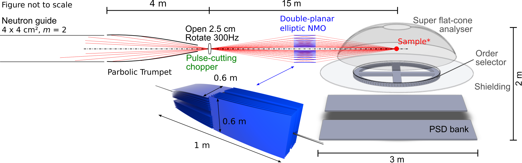
Figure 1: A not-to-scale overview of the instrument design. The neutrons are delivered by a neutron guide with an area of $40\times$40\text{\,}\mathrm{m}\mathrm{m}^{2}$$ from the reactor to a long ($4\text{\,}\mathrm{m}$) parabolic trumpet, which focuses the beam onto a small focal area. Here, a pulse cutting and shaping chopper system with openings of $10\times$10\text{\,}\mathrm{mm}$$ is located, defining the dynamical range and the energy resolution of the primary spectrometer. The elliptic NMO transports the neutrons emitted from the pulse-cutting chopper over a distance of $2f=$15\text{\,}\mathrm{m}$$ to the sample without distorting the phase-space. Above the sample the dome consisting of a large number of PG crystals is situated. This secondary spectrometer uses the principle of prismatic focusing the neutrons through an order selector onto the large position sensitive 2D detector (PSD).

3 Neutron transport

The prismatic focusing, a key feature of the instrument concept presented here, relies on illuminating a compact sample area, with the scattered signal being analysed by the super flat-cone analyser. Different mosaic blocks in the analyzer scatter to different positions on the position-sensitive detection system determining the final wave vector depending on the spot size of the beam at the sample and the resolution at the detector. Hence we limit the sample area to $10\,\times$$10\text{\,}\mathrm{m}\mathrm{m}^{2}$, which matches typical cross sections of single crystals, serving as the starting point for all subsequent considerations. While sensitive to the extent of the illuminated area, utilizing the prismatic focusing properties of the secondary spectrometer to first order decouples the instrument’s energy resolution from the initial beam’s divergence [12]. This observation invites the consideration of a modern neutron transport system tailored specifically towards small beams and large divergences. Rather recently, several of these concepts have been proposed and implemented. On the one hand, the Selene-type optics being based on two subsequent elliptic mirrors reducing the geometric aberrations, as implemented at the AMOR reflectometer at SINQ [13] and the ESS reflectometer ESTIA [14, 11]. It enables the imaging of a small beams extending $\leq$1\text{\,}\mathrm{mm}$$ in one direction with good brilliance transfer. On the other hand, we have explored the potential of elliptic nested mirror optics (NMO), essentially laterally nested short elliptic reflective surfaces, which provide good brilliance transfer while preserving the neutron phase space [15]. Furthermore, they allow tailoring the size and the divergence of the beam at the sample position by employing apertures close to the chopper system and close to the mirrors, respectively. Therefore we opted for such a NMO as shown in Fig. 1.

Considering the prismatic focusing properties of the secondary spectrometer, we aim for a maximum divergence of $2\times$2\text{\,}{}^{\circ}$$ at the sample position. Because of the timing requirements detailed in section 4, we opt for $15\text{\,}\mathrm{m}$ distance between the virtual source and the sample, immediately determining the focal length measured from the semi-minor axis of the ellipses $f=$7.5\text{\,}\mathrm{m}$$. By determining the maximum divergence and the distance between the common focal points of the elliptic reflective surfaces comprising the NMO, the geometry of the NMO transport system is fixed.

To redirect the neutron beam in two dimensions, i.e., vertical and horizontal transport, we require two orthogonally oriented NMOs, which are placed behind each other along the optical axis. This device is referred to as a double-planar elliptic NMO. As measured from the semi-minor axis, the mirrors of the vertically focusing device extend from $z=$-0.5\text{\,}\mathrm{m}$$ to $z=0$, and the horizontally focusing mirrors range from $z=0$ to $z=$0.5\text{\,}\mathrm{m}$$ along the optical axis, making the double-planar NMO $1\text{\,}\mathrm{m}$ long.

The combination of the desired divergence and the chosen focal length defines the required outermost semi-minor axis of the vertically and horizontally focusing NMO as follows $b_{\text{0, requ.}}=f\tan\left(\theta_{\text{max}}\right)\approx$0.26\text{\,}\mathrm{m}$$, yielding a beam cross-section of approximately $0.52\text{\,}\mathrm{m}$ incident on the NMO. To ensure that each neutron can interact with at least one mirror, also for possibly larger sources, the outermost semi-minor axes of the NMOs were chosen to be $b_{0}=$0.3\text{\,}\mathrm{m}$$.

Placing an aperture directly upstream of the double-planar device that restricts the illumination to the more central mirrors of the NMO enables tailoring the divergence of the beam distant to the sample.

Evidently, the NMO can only transport neutrons from the virtual source to the sample position, if the source is sufficiently illuminated with the required divergence and flux. This is achieved through a parabolic feeder, that focuses the low-divergence beam from the source to the maximum size of the virtual source. Due to the phase space preserving transport provided by the chosen NMO setup, the characteristics of the beam at the virtual source must match the requirements at the sample position, i.e. an extent of $10\times$10\text{\,}\mathrm{m}\mathrm{m}^{2}$$ and a divergence of $2^{\circ}\times 2^{\circ}$. While the small beam size at the sample position provides an excellent energy resolution of the secondary spectrometer, the small beam size at the virtual source enables the shaping of very short neutron choppers by disc choppers, so the primary spectrometer can nicely match the resolution the secondary.

As there is not yet a defined beam port or site for the instrument, we have included an exemplary transport section, connecting the the reactor source and the instrument. The beam is transported by a long $m=2$ guide with a constant square cross-section of $40\times$40\text{\,}\mathrm{m}\mathrm{m}^{2}$$. This guide is filled up to its acceptance which corresponds to $0.5^{\circ}\times 0.5^{\circ}$ collimation at $\lambda=2.5$ Å, which we consider the shortest wavelength for which we optimize this cold neutron spectrometer. This section can also be used to curve the beam and prevent the direct line of sight towards the reactor to realize a very low background level.

Figure 2 illustrates the characteristics of the neutron beam at various positions along the neutron guide.

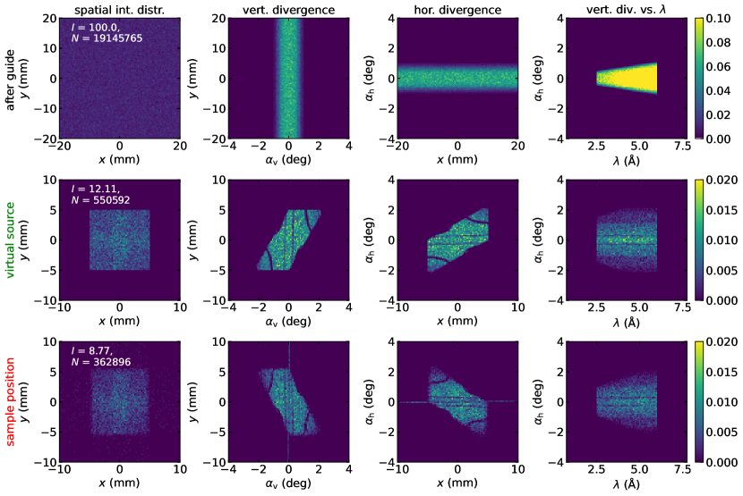
Figure 2: Simulated neutron distributions at various points along the instrument. The columns from left to right show, spatial intensity distributions, neutron intensity distributions as a function of position and divergence, along the vertical and horizontal directions, and the intensity as a function of the wavelength and the horizontal divergence, respectively. From top to bottom, the rows depict the distributions at the end of the long guide, at the virtual source after the parabolic trumpet, and at the sample position after the double planar NMO.

In the first row we show position, angle and wavelength distributions at the end of the straight section. The beam is as collimated as expected for the used supermirror coating and we can see the linear increase of the collimation as function of the wavelength $\lambda$. The second row shows the same distributions at the position of the virtual source. On realizes the distortions of the phase space due to the focusing feeder. The position distribution shows an enhanced intensity for the inner $\pm 1$ mm in both directions. The angle-position distributions have the overall shape of a parallelogram with some small gaps at very low angle and in the corner of the parallelogram. Still, within the region of interest for the instrument, the phase space is sufficiently homogeneous. In the third row, we show the distributions at the sample position. In particular, the spatial distribution at the virtual source and sample hardly differ, hence one can control the beam size far upstream, where the products of the neutron absorption do not increase the background level in the sample and detector area. The angle-position distributions have been mirrored at the position axis. Overall the intensity is reduced to 73% of the intensity at the virtual source, yielding a brilliance transfer that is competitive to other advanced neutron optics.

4 Chopper system

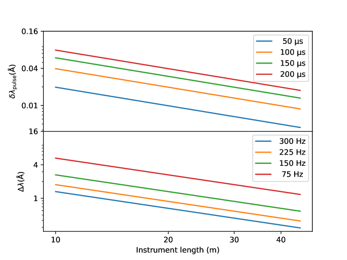
Figure 3: Primary wavelength resolution and bandwidth as a function of the instrument length for various pulse length $\tau_{\mathrm{P}}$ and repetition rate $f_{\mathrm{RR}}$.

At a continuous neutron source, such as the FRM II, a time-of-flight crystal analyzer spectrometer can control the pulse length, the timeframe and accordingly bandwidth by means of mechanical choppers labeled pulse shaping chopper (P), timeframe chopper (TF) and bandwidth chopper (BW). For a given instrument length $L$, the pulse length of the P-chopper assembly defines the primary wavelength resolution $\delta\lambda$ and in combination with the periodicity $T$ of the chopper system the dynamical range the primary neutron bandwidth $\Delta\lambda$:

$$\delta\lambda = \frac{h}{m_{n}}\frac{\tau_{\mathrm{P}}}{L}$$ (4.1)

$$\Delta\lambda = \frac{h}{m_{n}}\frac{T-\tau_{\mathrm{P}}}{L}\approx\frac{h}{m_{n}}\frac{1}{f_{\mathrm{RR}}L}.$$ (4.2)

The periodicity $T$ of the chopper system is the smallest common multiple of the individual chopper periodicities. In Fig. 3 we present typical combinations of resolution and bandwidth, that can be realized with state-of-the-art chopper technology as a function of the instrument length. Choosing an instrument length $L=15$ m we can vary the primary resolution between 0.012 Å  and 0.06 Å  i.e. close to the elastic line of the PG (002) analyzer. The primary energy resolution $\delta E/E$ can be varied between 0.5 and 2.5 %. At the same time, the band width can be adjusted between 0.9 and 4 Å. The low bandwidth is perfectly suited for investigations that focus a narrow spectral range of interest with high intensity, while the large bandwidth allows overview measurements in a wide spectral range making use of the most intense part of the cold neutron spectrum. As a special feature, the proposed chopper system decouples the pulse length and the repetition rate completely.

The implementation of short neutron pulses benefits strongly from the small beam cross section the NMO provides at the position of the P-chopper. For the beam of 10 mm$\times$ 10 mm, we can prepare the pulse length of 50 µs and above by 2 co-rotating chopper discs yielding a wavelength dependent pulse length [16, 17]. This is indicated in the time-wavelength acceptance diagram in the top left panel of Fig. 4, which have been introduced by Copley [18]. We use the center plane between the two P-chopper discs as the reference for the acceptance diagrams. Also the virtual source of the NMO, which is imaged onto the sample positions, lies in this plane. The colored areas indicate, at what time and wavelength neutrons cross the reference plane to be accepted by a chopper, i.e. they reach the chopper, when the transmission is $>0$. We chose time zero, when the beam is open for the chosen lowest wavelength $\lambda_{\mathrm{min}}$ of the requested band. The slope of the acceptance areas is proportional to the distance between the disc and the reference plane:

$$m=-\frac{m_{n}}{h}\times S.$$ (4.3)

Here $S$ indicates the position with respect to the plane containing the virtual source, which we consider also as the zero for the time-of-flight. Choppers upstream the reference plane feature a positive slope, and the choppers downstream accordingly a negative slope. As the two discs of the P-chopper group have the same distance from the reference plane, the absolute value $\absolutevalue{m}$ is the same. Neutrons can pass the chopper system only, when the accepted by all choppers of the system or when all colored regions overlap. In the top right panel of Fig. 4 we phase the 2 P-chopper discs such, that the downstream disc of the group opens the beam for neutrons with wavelength $\lambda_{\mathrm{min}}=2$ Å, while the upstream chopper terminates the pulse for this wavelength. For slightly larger wavelength the pulse length increases. The maximum pulse length that can can be realized is given by the width of the chopper window and the beam cross section. With the phase chosen in Fig. 4, it is achieved at $\lambda\approx 6.5\mathrm{\AA}$. Above this wavelength, the pulse length is decreasing with increasing wavelength. However, we can chose the phases of the choppers to realize any pulse length for a given neutron wavelength within this boundary. While we can control the pulse length of the P-chopper group via the phase of the choppers, the transmission is optimized, when we spin them at the highest possible speed. We consider here a maximum frequency $f_{\mathrm{max}}=300$ Hz, which can be safely realized using carbon fiber discs and magnetically driven choppers [11].

We also make use of the acceptance diagrams to determine the usable bandwidth of the instrument for a periodicity of the entire chopper system. This can be clarified from the bottom left panel of Fig. 4, which shows on period and one wavelength band. To increase the periodicity of the entire system from 3.333 ms to 10 ms, the timeframe chopper (TF) runs at a frequency of 200 Hz, while the P chopper frequency is 300 Hz. In black we draw here here lines, which indicate the acceptance of the analyzer surface at a distance $L_{\mathrm{Det}}=16$ m from the reference plane. We must be able to assign uniquely the time and wavelength of a neutron that has passed the reference plane and arrives at the analyzer. Hence we chose a lower wavelength $\lambda_{\mathrm{min}}$ which passes the reference plane at the end of the pulse, indicated by a black line. To assign this wavelength uniquely, the analyzer should stop accepting neutrons before the same wavelength from the next pulse arrive, which is indicated by the dashed black line. Therefore we reduced the periodicity by the pulse length, when we calculated the bandwidth in eq. 4.1. This acceptance line crosses the end of the original pulse at a wavelength $\lambda_{\mathrm{max}}=\lambda_{\mathrm{min}}+\Delta\lambda$, representing the bandwidth of the instrument graphically. To limit the band between this bounds we introduce the bandwidth chopper (BW), which has the periodicity of the P- and the TF-chopper system, e.g. 10 ms in the example in Fig. 4. Its acceptance is shown in the bottom panels of Fig. 4 as gray regions. Its window is chosen such, that it transmits only neutrons from the original pulse between the full and dashed black line as described above. It is defined by the position of the chopper with respect to the virtual source and the analyzer and the beam cross section at the position of the BW-chopper. Please note, that we placed the BW-chopper upstream of the virtual source. Usually the chopper is placed downstream the virtual source. Since the NMO result in a large cross section at the position of the chopper, we shifted it symmetrically to the other side of the virtual source, where the cross section of the feeding optics could be limited to 40 mm $\times$ 40 mm.

In the bottom right panel of Fig. 4 we inspect the transmission of the chopper system in a wider wavelength and time range to exclude contamination. Within this range common acceptance regions of all choppers exist only for $\lambda_{\mathrm{min}}<\lambda<\lambda_{\mathrm{max}}$. In particular the two discs of the P-chopper group will share acceptance regions only for $\lambda>100$ Å.

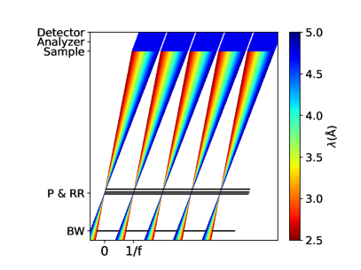
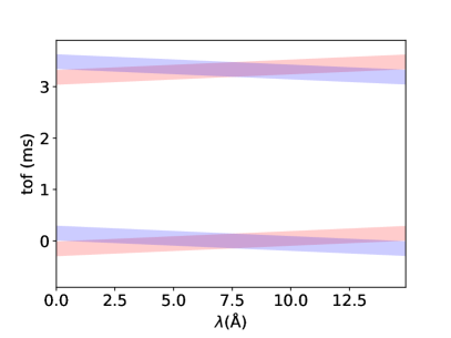
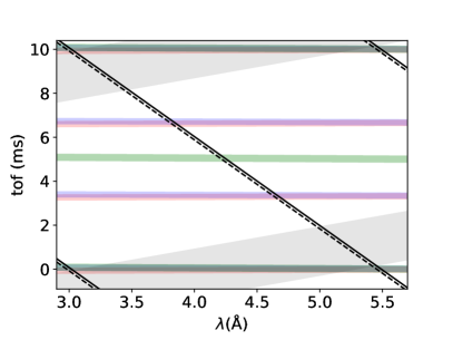
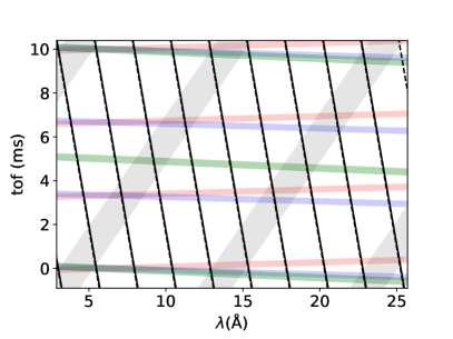
Figure 4: Top left: Flight path diagram of the instrument. Colors indicate the wavelength of the initial and analyzed neutrons, respecitively.Top right: Acceptance diagram with respect to the center of the pulse shaping chopper group consisting of 2 discs spinning at $f_{\mathrm{P}}=300$ Hz shown in light blue and red. Bottom left: Acceptance diagram of the full chopper system covering one timeframe and the first wavelength band. Bottom right: Acceptance diagram of the of the full chopper system covering the wavelength range $\lambda<30$ Å. Acceptance of the bandwidth chopper is shown in grey, The chosen frequency combination is $f_{\mathrm{P}}=300$ Hz, $f_{\mathrm{RR}}=100$ Hz, $f_{\mathrm{TF}}=200$ Hz.

The presentend chopper system provides continuous control of the pulse length via the phases of the P-chopper assembly, but also broad range of bandwidth and hence a flexible dynamic range. Changing the bandwidth hardly affects the sample flux as can be seen from Fig. 5. It shows the spectrum of a single chopper pulse at the sample position. Within the statistical limits of the simulation, the spectral intensity is the same for most of the bandwidth. The sample flux is given by the integration of the spectrum and then multiplication with the frequency. For a large frequency, the intensity is concentrated within a narrow dynamical range, while a large dynamical range is accessible for low frequency. For higher frequency, the edges of the transmitted spectrum are steeper,

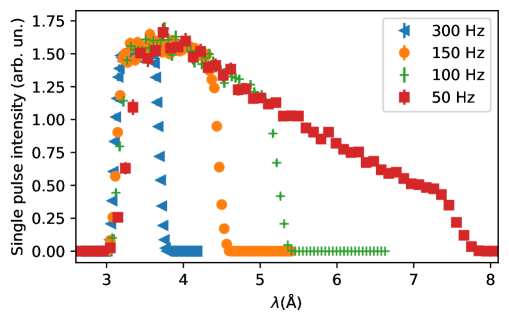
Figure 5: Single pulse wavelength spectrum at the sample position for different frequency of the BW-chopper. The P-chopper frequency is 300 Hz, the TF frequency is 300 hz, 150 Hz, 200 Hz and 250 Hz, respectively.

5 Secondary crystal spectrometer

5.1 Working principle

The secondary spectrometer with a mushroom-like super-flatcone analyser is the unique feature of the concept of a Mushroom spectrometer. The analyser consists of a large number of segments made of pyrolytic graphite (PG), reflecting the neutrons according to Bragg’s law after their interaction with the sample. The position of a segment is denoted by its azimuthal (horizontal) $\psi$ and polar (vertical) $\varphi$ angles with respect to the sample position. The angles and the wavenumbers in the coordinate system are illustrated in Fig. 6, while other components of the secondary spectrometer are shown in Fig. 1. Each analyser segment has a preset orientation, determining the scattering angle $\theta_{\mathrm{A}}$ at its $(\psi,\varphi)$ position. From the position of a neutron beam arriving at the position-sensitive detector (PSD) bank, the $(\psi,\varphi)$-information of the segment reflecting the beam can be determined, providing the orientation of the wavevector $\bm{k}_{\mathrm{f}}$ of the beam. Therefore, the complete information of the wavevector $\bm{k}_{\mathrm{f}}$ of the beam scattered by the sample can be resolved.

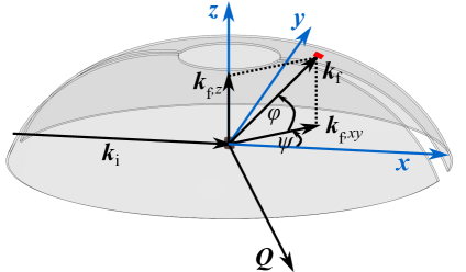
Figure 6: A schematic of the analyser illustrating the coordinate systems. The Cartesian system is defined with its origin at the sample position, the $z$-axis pointing upwards, the $x$-axis being parallel to the wavevector $\bm{k}_{\mathrm{i}}$ of incoming beam, and the $y$-axis completing a right-hand system. The analyser has a mirror symmetry with regard to the $xz$-and $yz$-planes, with the angular position $(\psi,\varphi)$-of one of its segments highlighted in red. For simplicity, the analyser is depicted as a singular entity on either side of the direct beam, adopting an elliptical form in a vertical sectional view. Consequently, the azimuthal angle $\psi$ signifies the angle between the wavevector $\bm{k}_{\mathrm{f}}$ of scattered beam and the $xz$-plane, while the polar angle $\varphi$ denotes the angle between $\bm{k}_{\mathrm{f}}$ and the $xy$-plane.

Since the reflection by the analyser has the contributions mainly from the diffraction orders PG 002 and 004, an order selector is implemented to select the diffraction order $n_{A}$ for determining the wavenumber $k_{\mathrm{f}}$ unambiguously. This is realised by using a mechanical velocity selector with a slit at the focal point of an elliptic curve in a vertical view, with the other focal point located at the sample position. The order selector is depicted in Fig. 7, with a radius $R$ and a thickness $D$. Each slit has a width $s$, an off-vertical angle $\beta$, and a phase distance $d=D\tan{\beta}$, which means that the time of the plate in the distance $d$ corresponds to the time of the neutron beam in the distance $D$. Denoting the rotation frequency $f$, the parameters are connected via $\frac{D}{v_{0}}=\frac{d}{2\pi Rf}$ or $\tan{\beta}=\frac{2\pi Rf}{v_{0}}$. The relative resolution can be expressed as

$$u_{\mathrm{r}}=\frac{s}{d}.$$ (5.1)

For distinguishing between the orders PG 002 and PG 004, a resolution of $u_{r}\approx$25\text{\,}\mathrm{\char 37\relax}$$ is already satisfactory.

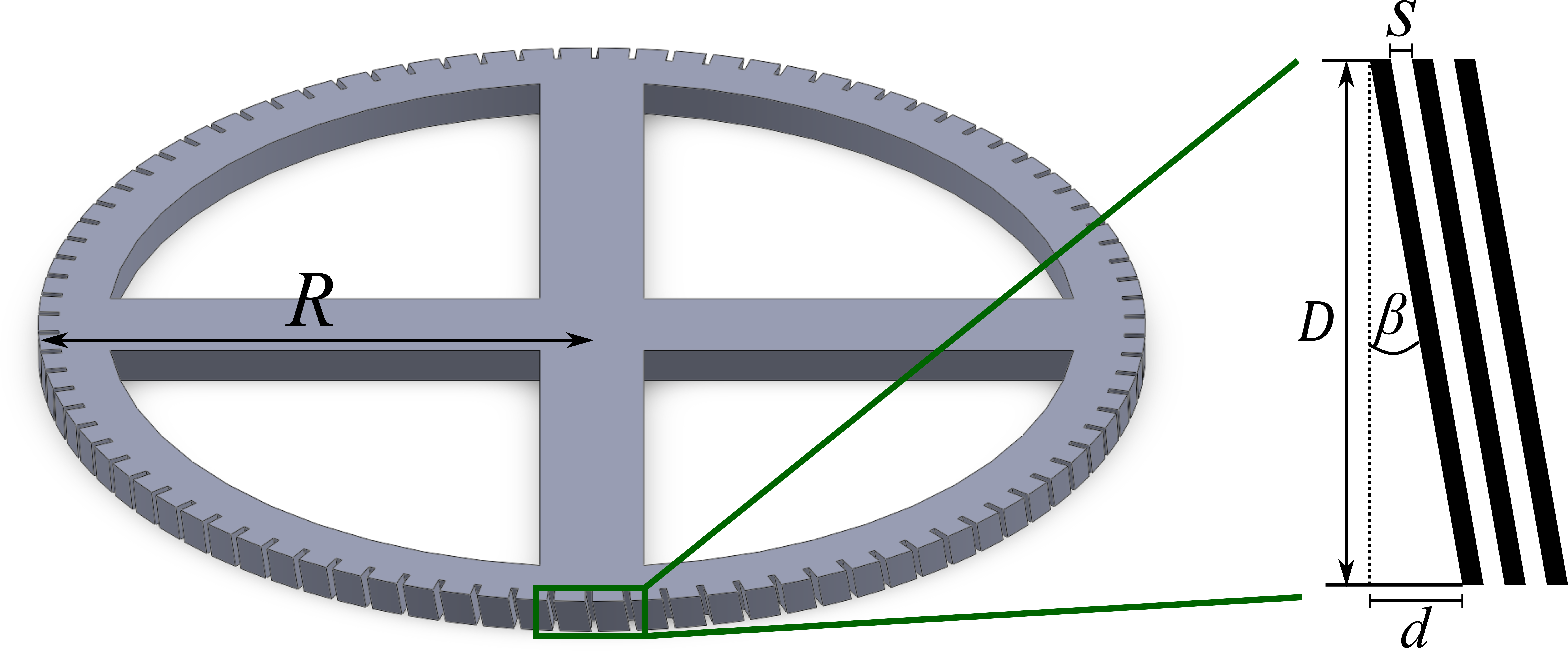
Figure 7: A simplified schematic of the order selector, featuring a radius $R$ and thickness $D$, for the secondary spectrometer of Mushroom. The size and number of slits are adjusted for the schematic to improve visibility, with the enlarged version illustrated on the right-hand side. The geometry of a slit is defined by its width $s$, tilting angle $\beta$, and phase difference $d=D\tan{\beta}$ between its two ends.

In order to decouple the wavenumber $k_{\mathrm{f}}$ and the vertical component $k_{\mathrm{f},z}$ of $\bm{k}_{\mathrm{f}}$, the analyser segments are positioned at distinct elliptic curves with constant focal points, such that the wavenumber $k_{\mathrm{f}}$ remains constant within the entire range of the vertical angle $\varphi$.

In order to keep a compact size of the secondary spectrometer and to offer a space for a cryostat with a diameter of $\geq$50\text{\,}\mathrm{cm}$$ at the centre, a geometry corresponding to $k_{\mathrm{f},002}=$1.1\text{\,}{\mathrm{\SIUnitSymbolAngstrom}}^{-1}$$ at PG 002 ($k_{\mathrm{f},004}=$2.2\text{\,}{\mathrm{\SIUnitSymbolAngstrom}}^{-1}$$) is chosen. With the configuration shown in Fig. 8, the analyser covers the angle $\varphi$ from $-5\text{\,}\mathrm{\SIUnitSymbolDegree}60\text{\,}\mathrm{\SIUnitSymbolDegree}$, and $\psi$ in the range of from $-170\text{\,}\mathrm{\SIUnitSymbolDegree}-10\text{\,}\mathrm{\SIUnitSymbolDegree}$ and from $10\text{\,}\mathrm{\SIUnitSymbolDegree}170\text{\,}\mathrm{\SIUnitSymbolDegree}$. The sample position is denoted as the centre $(0,0)$, and the other focal point is placed at $($0.4\text{\,}\mathrm{m}$,$-0.8\text{\,}\mathrm{m}$)$ in a vertical view. The PSD bank with the outer radius of $1.35\text{\,}\mathrm{m}$ is $1.24\text{\,}\mathrm{m}$ below the sample position. The spatial resolution of the PSD He-tubes is in the same order of magnitude as the size of analyser segments ($1\text{\,}\mathrm{cm}$). For the order selector, one can set $\gamma=$12\text{\,}\mathrm{\SIUnitSymbolDegree}$$, giving the frequency for PG 002 $f_{002}\approx$29.3\text{\,}\mathrm{Hz}$$ and for PG 004 $f_{004}\approx$58.6\text{\,}\mathrm{Hz}$$. With $s=$3\text{\,}\mathrm{mm}$$, one has $d=$12\text{\,}\mathrm{mm}$$ and $D\approx$56\text{\,}\mathrm{mm}$$.

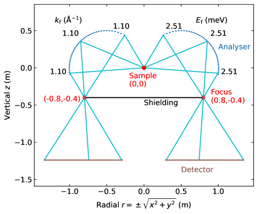
Figure 8: Schematic of the Mushroom secondary spectrometer in a sectional view. The dark blue dashed lines denote the analyser segments (every third segment is plotted for a better visual clarity), the light blue lines showcase some representative trajectories of the neutron beam, the brown lines illustrate the PSD banks, the black line indicates the shielding, and the red points depict the sample position at $(0,0)$ as well as the other focal points at $(\pm$0.8\text{\,}\mathrm{m}$,$-0.4\text{\,}\mathrm{m}$)$. The geometrical parameters correspond to a configuration for $k_{\mathrm{f}}=$1.1\text{\,}{\mathrm{\SIUnitSymbolAngstrom}}^{-1}$$ and $E_{\mathrm{f}}=$2.51\text{\,}\mathrm{meV}$$.

5.2 Resolution

The resolution of the secondary spectrometer of Mushroom can be characterised by three factors, the uncertainty of the wavenumber, $\Delta k_{\mathrm{f}}$, the angular spread of the wavevector $\bm{k}_{\mathrm{f}}$ in the horizontal plane, $\Delta\psi_{\mathrm{f}}$, and the angular spread in the vertical plane, $\Delta\varphi_{\mathrm{f}}$. Some geometrical contributions, for example an openning, can be expressed by a rectangular distribution, which is commonly approximated by a Gaussian distribution with the same standard deviation (SD) [19]. This allows the calculations of multiple contributions by using the propagation of uncertainty [20]:

$$\Delta f=\sqrt{\sum_{i=1}^{n}\left(\partialderivative{f}{x_{i}}\right)^{2}(\Delta x_{i})^{2}}.$$ (5.2)

Here, $\partialderivative{f}{x_{i}}$ represents the partial derivative of a function $f$ with respect to an independent variable $x_{i}$ . The uncertainty of $x_{i}$ is denoted by its SD, yielding: $\Delta x=\sigma_{x}$. Eq. 5.2 is valid when the SDs of all variables are small [21], which is true in most cases when discussing resolutions. Note that conversion is necessary when comparing a resolution characterised by its SD to a full width at half maximum (FWHM).

The analytical estimation of the wavenumber resolution, $\Delta k_{\mathrm{f}}$, can be derived from Bragg’s law, yielding:

$$\frac{\Delta k_{\mathrm{f}}}{k_{\mathrm{f}}}=\sqrt{\left(\frac{\Delta d}{d}\right)^{2}+\left(\cot{\theta_{\mathrm{A}}}\Delta\theta_{\mathrm{A}}\right)^{2}}.$$ (5.3)

The $d$-spacing of a PG crystal was determined by T. Keller et al. to exhibits a broadening of $\frac{\Delta d}{d}\lessapprox$2.5\text{\times}{10}^{-4}$$ (characterised by its SD) [22]. The uncertainty of scattering angle at an analyser, $\Delta\theta_{\mathrm{A}}$, are governed by various factors. Firstly, considering a fixed point on an analyser, an angular spread can be expressed as [23, 24]:

$$\Delta\theta_{\mathrm{A},1}=\sqrt{\frac{\alpha_{\mathrm{A,i}}^{2}\alpha_{\mathrm{A,f}}^{2}+\eta_{\mathrm{A}}^{2}\alpha_{\mathrm{A,i}}^{2}+\eta_{\mathrm{A}}^{2}\alpha_{\mathrm{A,f}}^{2}}{4\eta_{\mathrm{A}}^{2}+\alpha_{\mathrm{A,i}}^{2}+\alpha_{\mathrm{A,f}}^{2}}}.$$ (5.4)

where $\eta_{\mathrm{A}}$ denotes the mosaicity of the PG crystal used in the analyser and ranges typically from $0.13\text{\,}\mathrm{\SIUnitSymbolDegree}1.3\text{\,}\mathrm{\SIUnitSymbolDegree}$ (characterised by its SD) [25]. The incoming and outgoing divergences concerning the analyser are signified by $\alpha_{\mathrm{A,i}}$ and $\alpha_{\mathrm{A,f}}$, respectively, and can be estimated by considering the finite sizes of sample $l_{\mathrm{S}}$ and the opening of the focal point $l_{\mathrm{F}}$. Secondly, the deviation $\Delta\theta_{\mathrm{A},2}$ of scattering angles at different positions of the same analyser segment can be derived by considering the finite size of an analyser segment $l_{\mathrm{A}}$. With these two factors, the total angular spread at an analyser segment can be expressed as: $\Delta\theta_{\mathrm{A}}=\sqrt{\Delta\theta_{\mathrm{A},1}^{2}+\Delta\theta_{\mathrm{A},2}^{2}}$.

The angular spreads $\Delta\psi_{\mathrm{f}}$ (horizontal) and $\Delta\varphi_{\mathrm{f}}$ (vertical) of $\bm{k}_{\mathrm{f}}$ are governed by three factors. Firstly, the intrinsic resolution of the PSDs limits the smallest possible distance between two positions that can be resolved by the detector. Secondly, the beam divergence between the sample position and the analyser causes a deviation from the expected direction of $\bm{k}_{\mathrm{f}}$. Thirdly, possible overlaps between neutrons coming from neighbouring segments of analyser can cause an incorrect assignment of the $\bm{k}_{\mathrm{f}}$ direction.

In addition to analytical calculations, simulations were carried out using McStas, with both estimation methods considering $l_{\mathrm{S}}=l_{\mathrm{A}}=l_{\mathrm{F}}=$1\text{\,}\mathrm{cm}$$, depicted in Fig. 9. Here, the SD of the wavenumber $k_{\mathrm{f}}$ in percentage, as well as the radial ($\Delta r_{\mathrm{D}}$) and angular ($\Delta\psi_{\mathrm{D}}$) spreads on the PSD are compared, where $r_{\mathrm{D}}$ is the radial position on the detector defined in the the coordinate system as in Fig. 8, and $\psi_{\mathrm{D}}$ is defined in the same way as the horizontal angular position $\psi$ of analyser segments as in Fig. 6. This comparison is more direct than comparing the angular spreads $\Delta\psi_{\mathrm{f}}$ and $\Delta\varphi_{\mathrm{f}}$ of $\bm{k}_{\mathrm{f}}$, because converting the signals to $\Delta\psi_{\mathrm{f}}$ and $\Delta\varphi_{\mathrm{f}}$ involve the beam divergence between the sample and analyser. The analytical estimations of $\Delta r_{\mathrm{D}}$ and $\Delta\psi_{\mathrm{D}}$ do not involve the mosaicity $\eta_{\mathrm{A}}$ of analyser crystals.

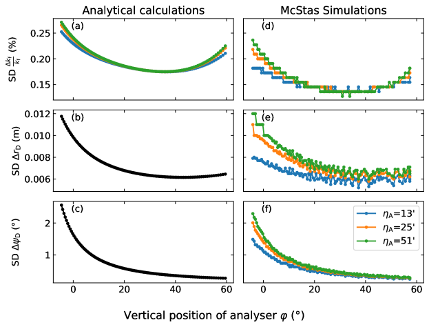
Figure 9: The $\bm{k}_{\mathrm{f}}$-resolution of the secondary spectrometer of the Mushroom, where the radial position is defined as $r=\pm\sqrt{x^{2}+y^{2}}$, with $x$ and $y$ defined in the Cartesian coordinate system in Fig. 6. Panels a and d: standard deviation (SD) of the wavenumber $k_{\mathrm{f}}$ in percentage. Panels b and e: SD of the radial position ($r_{\mathrm{D}}$) on the PSD. Panels c and f: SD of the angular position ($\psi_{\mathrm{D}}$) on the PSD. Panels a, b and c depict analytical calculations, while panels d, e and f present simulations using McStas. The values of mosaicity $\eta_{\mathrm{A}}$ of analyser crystals are labelled in colour, with the three SD values corresponding to $0.5\text{\,}\mathrm{\SIUnitSymbolDegree}$, $1\text{\,}\mathrm{\SIUnitSymbolDegree}$ and $2\text{\,}\mathrm{\SIUnitSymbolDegree}$ characterised by FWHM. The black curve in $\Delta r_{\mathrm{D}}$ and $\Delta\psi_{\mathrm{D}}$ indicate that the respective analytical calculations do not involve $\eta_{\mathrm{A}}$.

Fig. 9 shows a good agreement between the analytical calculations with simulations. The panels a and d indicate a very good wavenumber resolution of the secondary spectrometer, giving a relative uncertainty of about $0.2\text{\,}\mathrm{\char 37\relax}$. This is the case even with a relaxed mosaicity (FWHM) $\eta_{\mathrm{A}}\geq$1\text{\,}\mathrm{\SIUnitSymbolDegree}$$ of analyser crystals. The vertical spread $\Delta\varphi_{\mathrm{f}}$ is around $0.5\text{\,}\mathrm{\SIUnitSymbolDegree}$, while the horizontal spread $\Delta\psi_{\mathrm{f}}$ reaches $2\text{\,}\mathrm{\SIUnitSymbolDegree}$ when neutrons are reflected by the analyser segments with low $\varphi$. This results from the short distance between the analyser and the focal point at a low $\varphi$, which is about $0.4\text{\,}\mathrm{m}$ at the lowest segment. Besides, the neutrons coming from the analyser at a lower $\varphi$ arrive at the PSD with a smaller radial position, resulting in a larger angular spread than at a larger radial position considering the same tangential spread in length. This can be improved by implementing large crystals formed in the shape of circular stripe, which has a rotational symmetry at the same vertical position. With this, the horizontal spread $\Delta\psi_{\mathrm{f}}$ can be improved to below $1\text{\,}\mathrm{\SIUnitSymbolDegree}$. The mechanical possibility is under further investigation.

6 Conclusion

Here, we have investigated the potential of a time-of-flight crystal analyser spectrometer at a continuous neutron source. The instrument uses the large angular acceptance of PG to increase the count rate on the detector. At the same time a good energy resolution is achieved due to the good collimation realized by the illuminated sample size, the width of the individual analyzer crystals and the position resolution of the detector. Therefore the control of the beam spot size at the sample position is crucial for the energy and momentum resolution of the instrument. Thanks to the NMO, this beamspot size is effectively controlled at the position of the virtual source far upstream of the sample area. We have shown that we can effectively transport exactly the phase space element required by the instrument. So the NMO allows to limit the illumination to the sample only, preventing any background from neutrons that are scattered by the sample environment. Furthermore, all equipment needed to tailor the beam properties are far upstream. This gives excellent access to the sample area facilitating the operation of very complex sample environment, but also providing space for ancillary equipment, e.g. to control the state of the sample. But also the primary resolution benefits strongly from the NMO. It provides a natural position for the pulse shaping chopper. Thanks to the small cross section a trapezoidal transmission profile can be realized by a single chopper disc. As the pulse length requirements to match the secondary instrument resolution are well within the range, that can be realized by state-of-the-art chopper technology, we can use the concept of optical blind choppers. So we relax the pulse length for the longer wavelength in the band and compensate such the reduction of the source brightness towards longer wavelengths.

While the use of choppers seems counnter-intuitive on a continuous source such as the FRM II, it features distinct advantages for the study of dynamics in solids. By means of the repetititon rate we can control the bandwidth of the instrument freely. The bandwidth can be tuned from 0.8 Å to 4 Å. Tuning the lower limit of the bandwidth to the elastic line of the analyser, the instruments covers the dynamic range 0 meV $<\hbar\omega<20$ meV in the wide band configuration. If it is tuned symmetric to the elastic line in the narrow band configuration, the intensity is concentrated in the dynamic range -0.4 meV$<\hbar\omega<$ 0.4 meV, but can also be shifted to any other energy transfer range of interest. The bandwidth considerations are completely decoupled from the energy resolution requirements. Thanks to a narrow virtual source, the energy resolution can be controlled solely by the phase of the P choppers. The combination of the optics and the chopper system provides a sample flux, that reaches 10⁸ neutrons$/$cm${}^{2}/$s.

We are convinced, that this type of instrument with a huge acceptance of the analyser and a high sample flux in combination with a large accessible area around the sample will be useful for a wide range of applications in particular in the field of quantum and topological materials.

7 Acknowledgement

Intensive discussions about the crystal secondary mushroom concept with R. Bewley, ISIS are acknowledged very highly. This work was funded by the BMBF (German Federal Ministry for Research) under project number ErUM-Pro/05K19WOA.

References

- [1] D. Tennant, R. Cowley, S. Nagler and A. Tsvelik, Measurement of the spin-excitation continuum in one-dimensional using neutron scattering, Phys. Rev. B 52 (1995) 13368.
- [2] B.D. Piazza, M. Mourigal, N.B. Christensen, G.J. Nilsen, P. Tregenna-Piggott, T.G. Perring et al., Fractional excitations in the square-lattice quantum antiferromagnet, Nature Phys. 11 (2015) 62.
- [3] A. Banerjee, J. Yan, J. Knolle, C. Bridges, M.S. adn M.D. Lumsden, D. Mandrus et al., Neutron scattering in the proximate quantum spin liquid , Science 356 (2017) 105.
- [4] Y. Li, D. Adroja, D. Voneshen, R. Bewley, Q. Zhang, A. Tsirlin et al., Nearest-neighbour resonating valence bonds in , Nature Comm. 8 (2017) 15814.
- [5] S. Bramwell and M. Gingras, Spin ice state in frustrated magnetic pyrochlore materials, Science 294 (2001) 1495.
- [6] S. Mühlbauer, B. Binz, F. Jonietz, C. Pfleiderer, A. Rosch, A. Neubauer et al., Skyrmion lattice in a chiral magnet, Science 323 (2009) 915.
- [7] T. Weber, D. Fobes, J. Waizner, P. Steffens, G. Tucker, M. Böhm et al., Topological magnon band structure of emergent landau levels in a skyrmion lattice, Science 375 (2022) 1025.
- [8] Y.Shu, Q. Li, J. Xia, P. Lai, Z. Hou, Y. Zhao et al., Skyrmion-based reconfigurable logic gates and diodes in a racetrack with hard magnetic material and a notch, Journal of Magnetism and Magentic Materials 568 (2023) 170387.
- [9] X. Zang, Y. Zhou, M. Ezawa, G. Zhao and W. Zhao, Magnetic skyrmion transistor: skyrmion motion in a voltage-gated nanotrack, Science Report 5 (2015) 11369.
- [10] R. Bewley, The mushroom neutron spectrometer, NIM A 998 (2021) 165077.
- [11] K. Andersen, D. Argyriou, A. Jackson, J. Houston, P. Henry, P. Deen et al., The instrument suite of the european spallation source, NIM A 957 (2020) 163402.
- [12] J.O. Birk, M. Markó, P. Freeman, J. Jacobsen, R. Hansen, N.B. Christensen et al., Prismatic analyser concept for neutron spectrometers, Review of Scientific Instruments 85 (2014) 113908.
- [13] J. Stahn and A. Glavic, Focusing neutron reflectometry: Implementation and experience on the tof-reflectometer Amor, NIM A 821 (2016) 44.
- [14] J. Stahn, T. Panzner, U. Filges, C. Marcelot and P. Böni, Study on a focusing, low-background neutron delivery system, NIM A 634 (2011) S12.
- [15] C. Herb, O. Zimmer, R. Georgii and P. Böni, Nested mirror optics for neutron extraction, transport and focusing, NIM A 1040 (2022) 167154.
- [16] A. van Well, Double-disk chopper for neutron time-of-flight experiments, Physica B: Condensed Matter 180–181, Part 2 (1992) 959.
- [17] J. Voigt, N. Violini and W. Schweika, Compact chopper spectrometers for pulsed sources, Journal of Physics: Conference Series 746 (2016) 012018.
- [18] J.R.D. Copley, An acceptance diagram analysis of the contaminant pulse removal problem with direct geometry neutron chopper spectrometers, NIM A 510 (2003) 318.
- [19] A.M. Gaspar, Methods for analytically estimating the resolution and intensity of neutron time-of-flight spectrometers. the case of the toftof spectrometer, 0710.5319.
- [20] H.H. Ku, Notes on the use of propagation of error formulas, Journal of Research of the National Bureau of Standards C 70 (1966) 263.
- [21] A.A. Clifford, Multivariate error analysis, Wiley (1973).
- [22] T. Keller, M. Rekveldt and K. Habicht, Neutron larmor diffraction measurement of the lattice-spacing spread of pyrolytic graphite, Applied Physics A 74 (2002) S127.
- [23] J. Kalus and B. Dorner, On the use of in-pile collimators in inelastic neutron scattering, Acta Crystallographica Section A 29 (1973) 526.
- [24] M.T.F. Telling and K.H. Andersen, Spectroscopic characteristics of the OSIRIS near-backscattering crystal analyser spectrometer on the ISIS pulsed neutron source, Phys. Chem. Chem. Phys. 7 (2005) 1255.
- [25] M. Ohler, J. Baruchel, A.W. Moore, P. Galez and A. Freund, Direct observation of mosaic blocks in highly oriented pyrolytic graphite, NIM A 129 (1997) 257.