Exploring uniformity and maximum entropy distribution on torus through intrinsic geometry: Application to protein-chemistry

Abstract

A generic family of distributions, defined on the surface of a curved torus is introduced using the area element of it. The area uniformity and the maximum entropy distribution are identified using the trigonometric moments of the proposed family. A marginal distribution is obtained as a three-parameter modification of the von Mises distribution that encompasses the von Mises, Cardioid, and Uniform distributions as special cases. The proposed family of the marginal distribution exhibits both symmetric and asymmetric, unimodal or bimodal shapes, contingent upon parameters. Furthermore, we scrutinize a two-parameter symmetric submodel, examining its moments, measure of variation, Kullback-Leibler divergence, and maximum likelihood estimation, among other properties. In addition, we introduce a modified acceptance-rejection sampling with a thin envelope obtained from the upper-Riemann-sum of a circular probability density function, achieving a high rate of acceptance. This proposed sampling scheme will accelerate the empirical studies for a large-scale simulation reducing the processing time. Furthermore, we extend the Uniform, Wrapped Cauchy, and Kato-Jones distributions to the surface of the curved torus and implemented the proposed bivariate toroidal distribution for different groups of protein data, namely, $\alpha$-helix, $\beta$-sheet, and their mixture. A marginal of this proposed distribution is fitted to the wind direction data.

1 Introduction

The behavior of the observed data from a surface, or in general from a manifold, depends on the sampling scheme implemented for the collection of the data from that space. Statistical inference about the distribution of a manifold begins with sampling from it. Because of the availability of high dimensional dependent data, the statistical inferences on manifolds have been gaining more attention nowadays. [4], and [23] have discussed the development of mean and variance estimators on manifolds. [2], [30], and [7] have studied data on the projective space and sphere. The 2-dimensional curved torus, which is a Riemannian manifold embedded in $\mathbb{R}^{3}$ is particularly the interest of this paper. The bivariate von Mises density introduced by [18] is one of the popular toroidal distributions. Subsequently, numerous more parsimonious submodels have been proposed in the literature by authors such as [25], [28], [20], [16], and [1]. For an extensive overview of additional toroidal distributions, we direct interested readers to [see 17, Sec. 2.4 and Sec 2.5]. It’s worth noting that in the aforementioned studies, researchers have primarily focused on the flat torus, represented as $[0,2\pi)\times[0,2\pi)$. However, in the case of the curved torus, which considers the topology of it, has limited exploration. Specifically, there exists only one study addressing the uniform toroidal distribution, conducted by [5].

Inspired by the research of [5], we introduce a novel family of distributions tailored to the intrinsic geometry of a curved torus. Our investigation unfolds across several sections. In Section 2, we delve into the intrinsic geometry of the torus to comprehensively examine its properties. Utilizing the area element of the curved torus, introduced in Section 2, we proceed to Section 3, where we articulate a versatile family of distributions specifically designed on the surface of the curved torus.

In Section 4, we introduce a novel five-parameter family of distributions tailored to the surface of the curved torus. wherein we present a natural extension of the von Mises distribution, originally designed for circular distributions on the circle. In our construction of the general distribution on the surface of the curved torus, we observe that the distribution of the vertical angle, linked with the area element of the curved torus, holds greater significance compared to the distribution of the horizontal angle. Consequently, we dedicate extensive attention to the study of the three-parameter family of distribution of the vertical angle. This investigation encompasses the examination of the probability distribution function, exploration of special cases, and visualization of density graphs. Details of these analyses are presented in Sections 4.1 through 4.3. The von Mises distribution on the circle and the Fisher distribution on the sphere are intrinsic distributions that heavily rely on the area elements of their respective spaces. Both distributions are characterized as maximum entropy distributions within their respective spaces, subject to certain constraints. In a similar vein, the proposed distribution with the probability density function in Eq. 11 arises from the intrinsic geometry of the curved torus, where the area element plays a pivotal role. Analogous to the von Mises distribution on the circle and the Fisher distribution on the sphere, we demonstrate in Section 4.4 that under specific constraints, the proposed distribution with the probability density function outlined in Eq. 11 emerges as the maximum entropy distribution on the surface of the curved torus. In Section 4.5, we present the closed-form expressions for the trigonometric moments associated with the distribution. Furthermore, we dig into several key properties of the distribution described by the probability density function given in Eq. 11 in Sections 4.6 through 4.8. These properties include the conditions of symmetry, unimodality, and bimodality, as well as the divergence from the Cardioid distribution. Subsequently, in Section 4.9, we detail the process of maximum likelihood estimation (MLE) for the parameters of the model specified in Eq. 11. This involves considering the elements of both the observed and expected information matrices. It’s worth noting that our model necessitates the utilization of general numerical optimization methods to effectively implement maximum likelihood estimation.

We dedicate Section 5 to investigate the novel two-parameter family of symmetric and unimodal distributions associated with setting $\mu=0$ as the model described by Eq. 11 exhibits both symmetric and asymmetric characteristics depending on the parameter values. Here, we delve into various aspects of this symmetric sub-family, including its probability density function, moments, mode, anti-mode, Kullback-Leibler (KL) divergence, and maximum likelihood estimation, which are detailed in Sections 5.1 through 5.3. It’s noteworthy that the family of distribution proposed by [13] become very popular as the von Mises and Cardioid distributions are the special cases. In Section 5.4, we offer an extensive comparison between our proposed symmetric sub-family and the distributions introduced by [13], providing a comprehensive analysis of their similarities and differences.

In Section 6, in addition to the extension of the von Mises distribution, we provide a brief overview of the extension of other popular circular distributions, namely the Uniform, wrapped Cauchy, and Kato and Jones distributions, on the surface of a curved torus.

Inspired by the construction of the upper-Riemann-sum, in Section 7, we introduce a method to obtain a new envelope for acceptance-rejection sampling from many popular circular distributions. This method leverages a thin envelope around the target probability density function on a circle, resulting in a significantly high acceptance rate and reduced runtime compared to existing methods. For instance, in Section 1, we apply this new sampling method to the von Mises distribution and show its superiority with the existing method by [3]. Moreover, we extend this new sampling technique naturally to the torus. By adopting this method, we efficiently draw random samples from various distributions discussed in previous sections on the surface of the curved torus, achieving high acceptance rates. This proposed sampling scheme will accelerate the empirical inferential studies for a large-scale simulation.

In Section-8, we have done an extensive study of real data, for example, protein data of different groups as well as wind direction data described below.

1. Protein Data: The determination of the three-dimensional (3D) structure of a protein heavily depends on the precise characterization of torsion angles along the polypeptide chain, which consists of an ordered sequence of amino acids along the backbone comprising nitrogen and carbon atoms known as peptide units. The torsion angles, described by the $(\phi,\theta)$ angles, define the conformational landscape of proteins. In the literature of biochemistry, these pair of angles are often referred to as $(\phi,\psi)$. But for our convenience to maintain the flow of the paper and the conventional terminology of differential geometry, we use $(\phi,\theta)$ throughout this paper. These torsional angles, ranging from $-\pi$ to $\pi$, are essential for understanding protein secondary structures as well as classifications like $\alpha$-helices, $\beta$-sheets, and loop motifs, as showcased in Ramachandran plots. The significance of these plots extends to their toroidal data structure, prompting extensive research in density estimation, clustering, and dimension reduction techniques ([21], [6], [9], [26]). By studying these angles, researchers can gain valuable insights into the structural intricacies that underlie protein function and dynamics, paving the way for advancements in fields such as drug design, enzyme engineering, and molecular biology. It’s worth noting that the aforementioned studies on toroidal data are specifically focused on the flat torus $[0,2\pi)\times[0,2\pi)$.

   In the broader sense, proteins can be classified into three groups based on the predominant secondary structure, such as $\alpha-$helix, $\beta-$sheet, and a mixture of both. Among all these groups, the right-handed helix is common. For example, we consider the following proteins

   • 1A7D: This is a protein from the group of $\alpha-$helices. Figure-1(a) & (b) are the 3D structure and the Ramachandran plot of the Oxygen Transport protein, chloromet myohemerythrin (PDB ID-1A7D), respectively. (Source of the data is https://www.rcsb.org/).

   • 1SHG: This is a protein from the group of $\beta-$sheet. Figure-1(c) & (d) is the 3d structure and the Ramachandran plot of the Src- homologous SH3 domain (PDB ID-1SHG ), respectively. (Source of the data is https://www.rcsb.org/).

   • 2BNH: This is an average protein from the mixed group of $\alpha-$helix and $\beta-$sheet. Figure-1(e) & (f) is the 3D structure and the Ramachandran plot of the porcine ribonuclease inhibitor protein (PDB ID-2BNH), respectively. (Source of the data is https://www.rcsb.org/).

   

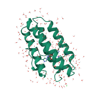
   (a)

   

   (b)

   

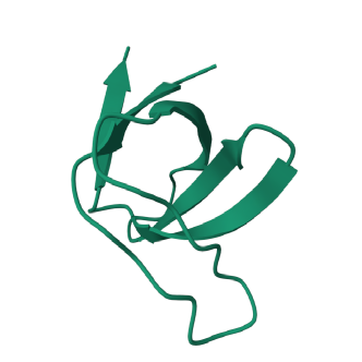
   (c)

   

   (d)

   

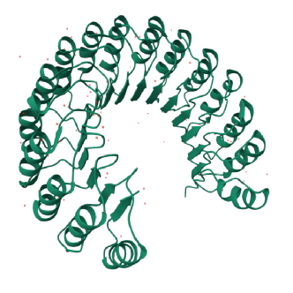
   (e)

   

   (f)

   Figure 1: The 3d representations and the corresponding Ramachandran plots of the Oxygen Transport protein, chloromet myohemerythrin ($\alpha$-helix), the Src- homologous SH3 domain ($\beta$-sheet), and porcine ribonuclease inhibitor protein (mix type) protein are in (a),(b); (c), (d); and (e), (f) repetitively (source of these images is: https://www.rcsb.org/).

2. Wind Direction Data: The direction of wind plays a pivotal role in shaping meteorological phenomena and climatic dynamics, impacting a myriad of sectors ranging from agriculture to urban planning and air quality management. Recognizing the intricacies of wind direction variability is paramount for applications such as renewable energy production, where wind patterns dictate the feasibility and efficiency of wind power generation. In this research paper, we delve into the modeling of wind direction variability specifically at Kolkata (Latitude 22.57, Longitude 88.36), the capital city of West Bengal, India. Spanning over four decades, from 1982 to 2023, our study focuses on the month of August, meticulously examining trends and fluctuations in wind direction to elucidate its implications on local weather patterns and climatic conditions.

The concluding Section-9 is succeeded by the necessary proofs provided in Appendix A.

2 Intrinsic geometry of torus

A torus is a geometric object representing two angular variables with respective radii. Only the angular part of it can be represented with a flat torus $[0,2\pi)\times[0,2\pi)$, but when the radii are involved, it is represented as the curved torus, see Eq. 1. The curved torus is not homeomorphic to the flat torus because their topological properties differ. To analyze the data represented on the surfaces of a curved torus, it is essential to have a proper notion of probability distributions it and statistical methodologies for the inference. The existing statistical techniques from the literature applicable to the flat torus do not apply to the analysis of data on a curved torus because it does not take into account the topology and geometry of the surface.

Here, we focus on the $2$-dimensional curved torus, a Riemannian manifold embedded in the $\mathbb{R}^{3}.$ In this report, we will use the term “curved torus” for $2$-dimensional curved torus. The parameter space for the curved torus is $\mathcal{S}=\{(\phi,\theta):0\leq\phi,\theta<2\pi\}$, and that can be represented in parametric equations as

$$x(\phi,\theta) =(R+r\cos{\theta})\cos{\phi}$$ (1)

$$y(\phi,\theta) =(R+r\cos{\theta})\sin{\phi}$$

$$z(\phi,\theta) =r\sin{\theta},$$

where $R,r$ are radii of the horizontal and vertical circles, respectively.

The parametric equation of $2$-dimensional torus in Eq. 1 is the Lipschitz image [see 5] of the set $\{(\phi,\theta):0<\phi,\theta<2\pi\}\subset\mathbb{R}^{2}.$ Clearly, the function $f(\phi,\theta)=\{(R+r\cos{\theta})\cos{\phi},(R+r\cos{\theta})\sin{\phi},r\sin{\theta}\}$ is a differentiable function from $\mathbb{R}^{2}$ to $\mathbb{R}^{3}$. Now, the partial derivatives of $f$ with respect to $\phi$, and $\theta$ are

$$\dfrac{\partial f}{\partial\phi}=\{-(R+r\cos{\theta})\sin{\phi},(R+r\cos{\theta})\cos{\phi},0\},$$

and

$$\dfrac{\partial f}{\partial\theta}=\{-r\sin{\theta}\cos{\phi},-r\sin{\theta}\sin{\phi},r\cos{\theta}\},$$

respectively. Hence, the derivative matrix is

$$Df(\phi,\theta)=\begin{bmatrix}-(R+r\cos{\theta})\sin{\phi}&-r\sin{\theta}\cos{\phi}\\ (R+r\cos{\theta})\cos{\phi}&-r\sin{\theta}\sin{\phi}\\ 0&r\cos{\theta}\end{bmatrix}.$$

Therefore, the Jacobian can be calculated as

$$J_{2}^{2}f(\phi,\theta)=\text{det}\left[D^{T}f(\phi,\theta)\cdot Df(\phi,\theta)\right]=\text{det}\begin{bmatrix}(R+r\cos{\theta})^{2}&0\\ 0&r^{2}\end{bmatrix}=r^{2}(R+r\cos{\theta})^{2}$$ (2)

Using the above expression of the square of the area element,[5] proposed to draw the samples $(\phi,\theta)$ from the probability density function given in Eq. 3 to ensure the uniformity with respect to area measure on the surface of a curved torus

$$g(\phi,\theta)=\dfrac{(1+\frac{r}{R}\cos{\theta})}{4\pi^{2}}=g_{1}(\phi)~{}g_{2}(\theta),$$ (3)

where

$$g_{1}(\phi)=\frac{1}{2\pi},~{}0\leq\phi<2\pi,$$ (4)

and

$$g_{2}(\theta)=\frac{1}{2\pi}\left[1+\frac{r}{R}\cos{\theta}\right],~{}0\leq\theta<2\pi.$$ (5)

The cumulative distribution function of $\theta$ is

$$G_{2}(\theta)=\frac{1}{2\pi}\left[\theta+\frac{r}{R}\sin{\theta}\right],~{}0\leq\theta<2\pi.$$

[5] use the acceptance-rejection sampling method for generating samples from the probability density function $g_{2}(\theta)$.

3 Construction of general distribution on the surface of the curved torus

Although several distributions on the flat torus have been introduced and studied by many researchers, only the distribution on the surface of the curved torus has been investigated by [5]. They have specially studied uniform distribution on torus given in Eq. 1 as an example of a manifold. In this section, we introduced a generalization for some popular distributions on the surface of a curved torus as an extension of circular distribution in higher dimensions.

Now, using the Eq. 2, we can determine the area element of the torus as $dA=r(R+r\cos{\theta})~{}d\phi d\theta.$ Hence, it is immediate that the area of the torus is given by

$$A=\int_{0}^{2\pi}\int_{0}^{2\pi}r(R+r\cos{\theta})\,\,d\phi\,d\theta=4\pi^{2}rR$$ (6)

Now, let us consider $\frac{r}{R}=\nu$, and a joint probability density function, $h(\phi,\,\theta)$ of $\phi$ and $\theta$, and from the Eq. 6 obtain the identity

$$4\pi^{2}rR = \int_{0}^{2\pi}\int_{0}^{2\pi}h(\phi,\,\theta)(2\pi r)(2\pi R)\,d\phi\,d\theta$$

$$= \frac{1}{C}\int_{0}^{2\pi}\int_{0}^{2\pi}h(\phi,\,\theta)\left(1+\nu\cos\theta\right)(2\pi r)(2\pi R)\,d\phi\,d\theta,$$

where $C$ is a normalizing constant, implying

$$1 = \frac{1}{C}\int_{0}^{2\pi}\int_{0}^{2\pi}h(\phi,\,\theta)\left(1+\nu\cos\theta\right)\,d\phi\,d\theta$$ (7)

$$= \frac{1}{C}\int_{0}^{2\pi}\int_{0}^{2\pi}h_{1}(\phi\,|\,\theta)\,\left[\,h_{2}(\theta)\left(1+\nu\cos\theta\right)\right]\,d\phi\,d\theta.$$

Here, in general, we can consider the following joint probability density function

$$h^{*}(\phi,\theta)=\frac{1}{C}\,h_{1}(\phi\,|\,\theta)\,\left[\,h_{2}(\theta)\left(1+\nu\cos\theta\right)\right],\mbox{~{}where~{}~{}}0\leq\phi,\theta<2\pi$$ (8)

In particular, when $\phi$ and $\theta$ are independently distributed then $h_{1}(\phi\,|\,\theta)\propto h_{1}(\phi)$. Hence, the Eq. 8 will reduce to

$$h^{*}(\phi,\theta)\propto h_{1}(\phi)\,\left[h_{2}(\theta)\left(1+\nu\cos\theta\right)\right],\mbox{~{}where~{}~{}}0\leq\phi,\theta<2\pi.$$ (9)

4 von Mises distribution on the surface of the curved torus

It’s commonly noted that distributions on a flat torus often display symmetry around its location. However, real-world datasets don’t always conform to this pattern, as pointed out by [27] in their study of orthologous genes in circular prokaryotic genomes. This emphasizes the need for developing distributions capable of accommodating asymmetry to effectively model such datasets. Consequently, there’s a considerable demand for asymmetric distributions on curved torus.

In this section, we proposed the extension of the von Mises distribution on the surface of the curved torus. Let $\phi$ and $\theta$ be independently von Mises distributed on the flat torus with concentration parameters $\kappa_{1}$, $\kappa_{2}$, and location parameters $\mu_{1}$, $\mu_{2}$, respectively. So, now, using Eq. 8 we can define the following new distribution as

$$h^{*}(\phi,\theta)=\frac{e^{\kappa_{1}\cos(\phi-\mu_{1})}}{2\pi I_{0}(\kappa_{1})}\left[\frac{e^{\kappa_{2}\cos(\theta-\mu_{2})}}{C}\left(1+\nu\cos\theta\right)\right],$$ (10)

where $0\leq\phi,\theta<2\pi$, $0\leq\mu_{1},\mu_{2}<2\pi$, $\kappa_{1},\kappa_{2}>0$, which implies

$$h_{1}(\phi)=\frac{e^{\kappa\cos(\phi-\mu_{1})}}{2\pi I_{0}(\kappa_{1})}\mbox{~{}and~{}}h^{*}_{2}(\theta)=\frac{e^{\kappa_{2}\cos(\theta-\mu_{2})}}{C}\left(1+\nu\cos\theta\right),$$

with

$$C=2\pi\left[I_{0}(\kappa_{2})+\nu\cos\mu_{2}~{}I_{1}(\kappa_{2})\right]$$

is the normalizing constant (see, Appendix-A.1).Thus, the joint probability density function described in Eq. 10 characterizes the von Mises distribution on the surface of a curved torus, typically exhibiting asymmetry and bimodality. Figure-2(a) $\&$ (b) illustrate the bivariate symmetric probability density function for $(\mu_{1},\mu_{2})=(0,0)$, while Figure-2(c) $\&$ (d) depict the bivariate asymmetric probability density function for $(\mu_{1},\mu_{2})=(0,\pi)$. Throughout these representations, the parameters remain same: $(\kappa_{1},\kappa_{2})=(1.5,2.5)$ and $\nu=0.8$.

Note that the probability density function, $h_{1}(\phi)$ of horizontal angle $\phi$ is the von Mises distribution. Many researchers have already studied this distribution in great detail [see 19, 12]. In the following section, we extensively studied the probability density function, $h^{*}_{2}(\theta)$ of the vertical angle $\theta$ because it involves both the density of the von Mises distribution as well as the area element of the curved torus.

4.1 Marginal density on vertical cross-sectional circle

The probability density function of the vertical angle $\theta$ is

$$h^{*}_{2}(\theta)=\frac{e^{\kappa\cos(\theta-\mu)}\left(1+\nu\cos\theta\right)}{2\pi(I_{0}(\kappa)+\nu\cos\mu~{}I_{1}(\kappa))},$$ (11)

where, $\theta,\mu\in[0,2\pi)$, $\kappa>0$, and $\nu\in(0,1).$

4.2 Special Cases

Some special cases can be derived from the probability density function in Eq. 11.

• von Mises: As $\nu\xrightarrow{}0$ the Eq. 11 becomes $h^{*}_{2}(\theta)=\frac{e^{\kappa\cos(\theta-\mu)}}{2\pi~{}I_{0}(\kappa)}$, which is the probability density function of von Mises distribution.

• Cardioid: When $\kappa=0$, $I_{0}(0)=1\mbox{~{}and~{}}I_{1}(0)=0$. Hence the Eq. 11 becomes $h^{*}_{2}(\theta)=\frac{1}{2\pi}\left(1+\nu\cos\theta\right)$ , which is the probability density function of Cardioid distribution with location parameter at $\eta=0$ [see 19].

• Uniform: As $\nu\xrightarrow{}0$, and $\kappa=0$, the Eq. 11 becomes $h^{*}_{2}(\theta)=\frac{1}{2\pi}$ , which is the probability density function of circular uniform distribution.

• Dirac-delta distribution: As $\kappa\rightarrow\infty$, the model in Eq. 11 represents a one-point distribution for all $\nu$ with singularity at $\theta=\mu.$

4.3 Visualizing densities

Now let $\mu_{1}=\mu_{2}=0$, $\kappa_{1}=\kappa_{2}=1$, and $r=1.5,~{}R=3.$ then the Figure-5(b) is the histogram of the sampled data drawn from the probability density function of the vertical angle $\theta$ using the newly proposed sampling method in Section-7. In this section, we further discuss the interpretation of the parameters by making some plots of probability density functions. Following Eq. 11 Figure-3(a) is obtained by putting $\mu=\frac{\pi}{2},\nu=0.5$, and varying $\kappa$ from $0$ to $4$ with each increment $1$. Note that for $\kappa=0$ it provides the plot of Cardioid distribution. Figure-3(b) is obtained by putting $\mu=\frac{\pi}{2},\kappa=1$, and varying $\nu$ from $0.1$ to $0.4$ in steps of $0.1$. We can see that from Figure-3(a) $\&$ Figure-3(b) that the density is asymmetric in general. Figure-3(c) is obtained by putting $\nu=0.5,\kappa=1$, and $\mu=0,\frac{\pi}{3},\frac{2\pi}{3},\pi.$ The Figure-3(c) shows the interpretation of $\mu$, implying that the parameter $\mu$ has a crucial role in controlling the skewness of the model.

4.4 The maximum entropy characterization

The maximum entropy characterizations of the toroidal distributions having the probability density function described by Eq. 11 can be derived through an extension of the general result provided by [14] . This result has been applied to the von Mises distribution on the circle and the Fisher distribution on the sphere by [18, pp. 65-66] and [24, pp. 162-163], respectively.

The maximum entropy distribution on the circle is von Mises distribution having the probability density function in Eq. 42, and the maximum entropy distribution on the sphere is the Fisher distribution due to [8] having the probability density function.

$$f_{f}(\phi,\theta)=\frac{1}{2\pi}\frac{\kappa}{2\sinh\kappa}e^{\kappa\cos\theta}\sin\theta,$$ (12)

where $\kappa>0,0\leq\theta<\pi$, and $0\leq\phi<2\pi.$ It is important to note that the probability density function for the azimuthal angle (horizontal) and zenith angle (vertical angle) is $h^{s}_{1}(\phi)=\frac{1}{2\pi}$ and $h^{s}_{2}(\theta)=\frac{\kappa}{2\sinh\kappa}e^{\kappa\cos\theta}\sin\theta,$ respectively. Also, the Jacobian for the unit sphere is $J_{s}=\sin\theta$, which is associated with the vertical angle. For a more detailed explanation of spherical distribution, the reader may refer to [19] .

From the above discussion of the Fisher distribution and its maximum entropy characterization, it can be observed that the distribution of the vertical angle plays a crucial role in the sphere. Similar can be observed for the toroidal distribution also. Here, we deduce the maximum entropy characterization of toroidal distribution in the following theorem.

Theorem 1.

The marginal density of the maximum entropy distribution for the vertical angle $\theta$ on the curved torus is given in Eq. 11, subject to the constraints,

$$E(\cos\theta) = a_{1}$$ (13)

$$E(\sin\theta) = a_{2}$$ (14)

$$E\left(\log(J_{2}(f(\phi,\theta)))\right) = a_{3},$$ (15)

where,

$$a_{1} = \frac{I_{1}(\kappa)}{I_{0}(\kappa)}\cos\mu,~{}~{}~{}~{}a_{2}=\frac{I_{1}(\kappa)}{I_{0}(\kappa)}\sin\mu,$$

$$a_{3} = \displaystyle\sum_{t=1}^{n}\left[(-1)^{(t+1)}\left(\frac{\nu I_{t-1}(\kappa)+2~{}I_{t}(\kappa)+\nu I_{t+1}(\kappa)}{2\left[I_{0}(\kappa)+\nu\cos\mu~{}I_{1}(\kappa)\right]}\right)\cos t\mu\right]$$

Proof.

See the Appendix-A.2 for the proof. ∎

Remark 1.

If the distribution for the horizontal angle $\phi$ is the circular uniform distribution with probability density function $h_{1}(\phi)=\frac{1}{2\pi}$ for $0\leq\phi<2\pi,$ together with $h^{*}_{2}(\theta)$ for vertical angle $\theta$ as in Eq. 11, the probability density function of the maximum entropy distribution on curved torus is

$$h^{*}(\phi,\theta)=\frac{1}{2\pi}\left[\frac{e^{\kappa\cos(\theta-\mu)}}{\left[2\pi(I_{0}(\kappa)+\nu\cos\mu~{}I_{1}(\kappa))\right]}\left(1+\nu\cos\theta\right)\right],$$

where $0\leq\phi,\theta<2\pi$, $0\leq\mu<2\pi$, $\kappa>0$. Here, $h_{1}(\phi)=\frac{1}{2\pi}$ is the maximum entropy distribution without any restrictions.

Remark 2.

If the distribution of the horizontal angle $\phi$ is the von Mises distribution with the probability density function provided in Eq. 42, together with $h^{*}_{2}(\theta)$ for vertical angle $\theta$ as in Eq. 11, the probability density function of the maximum entropy distribution on the curved torus is

$$h^{*}(\phi,\theta)=\frac{e^{\kappa_{1}\cos(\phi-\mu_{1})}}{2\pi I_{0}(\kappa_{1})}\left[\frac{e^{\kappa_{2}\cos(\theta-\mu_{2})}}{\left[2\pi(I_{0}(\kappa_{2})+\nu\cos\mu_{2}~{}I_{1}(\kappa_{2}))\right]}\left(1+\nu\cos\theta\right)\right],$$

where $0\leq\phi,\theta<2\pi$, $0\leq\mu_{1},\mu_{2}<2\pi$, $\kappa_{1},\kappa_{2}>0$. Here, $h_{1}(\phi)=\frac{e^{\kappa_{1}\cos(\phi-\mu_{1})}}{2\pi I_{0}(\kappa_{1})}$ is the probability density function of the maximum entropy distribution on circle subject to the restrictions :

$$E(\cos\phi) = \frac{I_{1}(\kappa_{1})}{I_{0}(\kappa_{1})}\cos\mu_{1},~{}~{}~{}~{}E(\sin\phi)=\frac{I_{1}(\kappa_{1})}{I_{0}(\kappa_{1})}\sin\mu_{1},$$

4.5 Trigonometric Moments

The trigonometric moments of the probability density function in Eq. 11 are given by the following theorem:

Theorem 2.

If $\Theta\sim h^{*}_{2}(\theta)$ in Eq. 11 then the $p^{th}$ trigonometric moments for $p=0,\pm 1,\pm 2,\ldots$ are given by

$$\Phi_{p}=\frac{\nu I_{p-1}(\kappa)e^{i(p-1)\mu}+2I_{p}(\kappa)e^{ip\mu}+\nu I_{p+1}(\kappa)e^{i(p+1)\mu}}{2\left[I_{0}(\kappa)+\nu\cos\mu~{}I_{1}(\kappa)\right]}$$

Proof.

See the Appendix-A.3 for the proof. ∎

Corollary 1.

As $\nu\rightarrow 0$ the $pth$ trigonometric moments for $p=0,\pm 1,\pm 2,\ldots$ in Theorem-2 becomes

$$\Phi_{p}=\frac{I_{p}(\kappa)e^{ip\mu}}{I_{0}(\kappa)},$$

which is the $pth$ trigonometric moments for von Mises distribution.

Corollary 2.

When $\kappa=0$ the $pth$ trigonometric moments for $p=0,\pm 1,\pm 2,\ldots$ in Theorem-2 becomes

$$\Phi_{p}=\frac{\nu I_{p-1}(0)e^{i(p-1)\mu}+2~{}I_{p}(0)e^{ip\mu}+\nu I_{p+1}(0)e^{i(p+1)\mu}}{2\left[I_{0}(0)+\nu\cos\mu~{}I_{1}(0)\right]},$$

as $I_{p+1}(0)=I_{p-1}(0)=0,\mbox{~{}for~{}}p\neq\pm 1$ $\mbox{~{}and~{}}I_{0}(0)=1,$ then we can write trigonometric moments as

$$\Phi(\theta)=\frac{\nu}{2},$$

which is the $pth$ trigonometric moments for Cardioid distribution with location parameter $\eta=0$, for more details [see 12].

4.6 Condition of Symmetry

The probability density function in Eq. 11 is generally an asymmetric distribution. Hence, the condition for the symmetry is given in the following corollary

Corollary 3.

The probability density function in Eq. 11 is symmetric iff $\mu=0$, $\kappa=0$ or $\nu\xrightarrow{}0$.

Proof.

See Appendix-A.4, for the proof. ∎

Of course, the symmetric special cases with $\nu\xrightarrow{}0$ and $\kappa=0$ are the von Mises and Cardioid distributions; the wider two-parameters family of symmetric distributions arising when $\mu=0$ as discussed in Section 5.

4.7 Condition of Modality

The probability density function in Eq. 11 can be both unimodal or multimodal depending on the parameters $\mu$, $\kappa$ and $\nu$ . In this subsection, we give necessary and sufficient conditions for unimodality. Here the proposed probability density function is differentiable with respect to $\theta\in[0,2\pi).$ Now, the derivative of Eq. 11 with respect to $\theta$ is

$$\frac{d}{d\theta}h^{*}_{2}(\theta) \propto \frac{d}{d\theta}\left[e^{\kappa\cos{(\theta-\mu)}}\left(1+\nu\cos{(\theta)}\right)\right]$$ (16)

$$= -{\kappa}\mathrm{e}^{{\kappa}\cos\left({\theta}-{\mu}\right)}\cdot\left(1+\nu\cos\left({\theta}\right)\right)\sin\left({\theta}-{\mu}\right)-\nu\mathrm{e}^{{\kappa}\cos\left({\theta}-{\mu}\right)}\cdot\sin\left({\theta}\right)$$

To identify the number of modes we need to solve the following equation $\frac{d}{d\theta}h^{*}_{2}(\theta)=0$ which implies that

$$-{\kappa}\mathrm{e}^{{\kappa}\cos\left({\theta}-{\mu}\right)}\cdot\left(1+\nu\cos\left({\theta}\right)\right)\sin\left({\theta}-{\mu}\right)-\nu\mathrm{e}^{{\kappa}\cos\left({\theta}-{\mu}\right)}\cdot\sin\left({\theta}\right)=0$$ (17)

simplifying to

$$b_{1}\left[\sin{\theta}+\nu\cos{\theta}\right]-b_{2}\left[\cos{\theta}+\nu\cos^{2}{\theta}\right]+b_{3}\sin{\theta=0},$$ (18)

where, $b_{1}=\cos{\mu},b_{2}=\sin{\mu},\mbox{~{}and~{}}b_{3}=\frac{\nu}{\kappa}$

As discussed in a related context by [31], this equation is equivalent to four degree equation which can be obtained by the transformation $x=\tan(\theta/2)$, so we can use

$$\sin\theta=\frac{2x}{1+x^{2}},\mbox{~{}and~{}}\cos\theta=\frac{1-x^{2}}{1+x^{2}}$$

in the Eq. 18, hence it becomes

$$d_{4}x^{4}+d_{3}x^{3}+d_{2}x^{2}+d_{1}x+d_{0}=0,$$ (19)

where $d_{4}=b_{2}(1+\nu),d_{3}=2b_{3}+2b_{1}(1-\nu),d_{2}=2b_{2}\nu,d_{1}=2b_{3}+2b_{1}(1+\nu)\mbox{~{}and~{}}d_{0}=b_{2}(\nu-1).$ This quartic equation can be solved using Ferrari’s method, as discussed by [29]. The discriminant of this equation is

$$\Delta = d_{0}^{2}\left[-27d_{3}^{4}+144d_{2}d_{3}^{2}d_{4}-128d_{2}^{2}d_{4}^{2}-192d_{1}d_{3}d_{4}^{2}\right]$$ (20)

$$+ d_{0}\left[-4d_{2}^{3}d_{3}^{2}+18d_{1}d_{2}d_{3}^{3}+16d_{2}^{4}d_{4}-80d_{1}d_{2}^{2}d_{3}d_{4}-6d_{1}^{2}d_{3}^{2}d_{4}+144d_{1}^{2}d_{2}d_{4}^{2}\right]$$

$$+ d_{1}^{2}d_{2}^{2}d_{3}^{2}-4d_{1}^{3}d_{3}^{3}-4d_{1}^{2}d_{2}^{3}d_{4}+18d_{1}^{3}d_{2}d_{3}d_{4}-27d_{1}^{4}d_{4}^{2}+256d_{0}^{3}d_{4}^{3}$$

Eq. 19 is known to have four real roots or four complex roots if $\Delta>0$, and two real roots and two complex roots if $\Delta<0$. This ensures that the probability density function has no more than two modes. Moreover, the distribution is bimodal when $\Delta>0$ and unimodal when $\Delta<0$. Because $d_{i},i=1,\cdots,4$, are functions of $\mu,\kappa,\mbox{~{}and~{}}\nu$ the conditions for unimodality can in principle be written out in terms of these three parameters.

Remark 3.

When $\mu=0$ then $b_{1}=1,b_{2}=0$, and $b_{3}=\frac{\nu}{k}$. Eventually $d_{4}=d_{2}=d_{0}=0,d_{3}=\frac{2\nu}{\kappa}+2(1-\nu)$, and $d_{1}=\frac{2\nu}{\kappa}+2(1+\nu)$. So, the Eq. 19 becomes

$$d_{3}x^{3}+d_{1}x=0$$ (21)

with the discriminant $\Delta=-4d_{3}d_{1}^{3}$. Now, we have $\kappa>0$, and $\nu\in(0,1)$, hence $d_{1},d_{3}$ are always positive and as a consequence, the discriminant $\Delta=-4d_{3}d_{1}^{3}$ is always negative. Thus, the probability density function in Eq. 11 is unimodal for $\mu=0.$ The Figure-3(c) also agrees with this.

Remark 4.

When $\mu=\pi$ then $b_{1}=-1,b_{2}=0$, and $b_{3}=\frac{\nu}{\kappa}$. Eventually $d_{4}=d_{2}=d_{0}=0,d_{3}=\frac{2\nu}{\kappa}-2(1-\nu)$, and $d_{1}=\frac{2\nu}{\kappa}-2(1+\nu)$, so, $d_{1},d_{2}$ can be positive or negative depending upon the values of $\kappa>0$, and $\nu\in(0,1)$.

Similarly, as above, we can have the following discriminant $\Delta=-4d_{3}d_{1}^{3}$. The bimodality and unimodality depend on the sign of the $d_{1},d_{3}.$ Let us consider the following cases:

• Case-1: when $d_{1},d_{3}<0$, we have $\Delta<0$ which implies unimodality. Now, $d_{1}<0\implies\kappa>\frac{\nu}{1+\nu}$, and $d_{3}<0\implies\kappa>\frac{\nu}{1-\nu}$. Together it gives the unimodality if $\kappa>\frac{\nu}{1-\nu}$.

• Case-2: when $d_{1},d_{3}>0$, we have $\Delta<0$ which implies unimodality. Now, $d_{1}>0\implies\kappa<\frac{\nu}{1+\nu}$, and $d_{3}>0\implies\kappa<\frac{\nu}{1-\nu}$. Together it gives the unimodality if $\kappa<\frac{\nu}{1+\nu}$.

• Case-3: when $d_{1}<0$ and $d_{3}>0$, we have $\Delta>0$ which implies bimodality. Now, $d_{1}<0\implies\kappa>\frac{\nu}{1+\nu}$, and $d_{3}>0\implies\kappa<\frac{\nu}{1-\nu}$. Together, it gives the bimodality if $\frac{\nu}{1+\nu}<\kappa<\frac{\nu}{1-\nu}$.

• Case-4: when $d_{1}>0$ and $d_{3}<0$, we have $\Delta>0$ which implies bimodality. Now, $d_{1}>0\implies\kappa<\frac{\nu}{1+\nu}$, and $d_{3}<0\implies\kappa>\frac{\nu}{1-\nu}$. Since, $\nu\in(0,1)$ thus, this case is not possible.

In particular, we have chosen $\nu=0.9$, so $\frac{\nu}{1+\nu}=0.4736842$, and $\frac{\nu}{1-\nu}=9$. Therefore, from Figure-3(d), we can see that when $\kappa=9,10,0.4736842$, and $0.3$, then the probability density function in Eq. 11 is unimodal which agrees with the Case-1, and Case-2.When $0.4736842<\kappa<9$, that is $\kappa=3.3157895,6.1578947$, then the probability density function in Eq. 11 is bimodal which agrees with the Case-3.

4.8 Divergence From the Cardioid Distribution

In this section, we compare the probability density function as given in Eq. 11 with the probability density function of the Cardioid distribution through KL divergence

$$f_{c}(\theta)=\frac{1}{2\pi}\left(1+\nu\cos\theta\right)$$ (22)

where $\nu\in(0,1).$ Calculating the KL divergence between $h^{*}_{2}$ and $f_{c}$ we get

$$D_{KL}(f_{c},h^{*}_{2}) = \log((I_{0}(\kappa)+\nu\cos\mu~{}I_{1}(\kappa)))-\frac{\nu\kappa~{}\cos\mu}{2},$$ (23)

see A.5 in Appendix for details. Clearly $D_{KL}(f_{c},h^{*}_{2})=0$ for $\kappa=0$. To understand the sensitivity of $D_{KL}$ with respect to $\kappa$, we consider

$$\frac{\partial D_{KL}(f_{c},h^{*}_{2})}{\partial\kappa} = \frac{I_{1}(\kappa)+\nu\cos\mu~{}[I_{0}(\kappa)+I_{2}(\kappa)]}{(I_{0}(\kappa)+\nu\cos\mu~{}I_{1}(\kappa))}-\frac{\nu\cos\mu}{2}$$

$$= \frac{A(\kappa)+\nu\cos\mu~{}[1+1-\frac{2A(\kappa)}{\kappa}]}{(1+\nu\cos\mu~{}A(\kappa))}-\frac{\nu\cos\mu}{2},$$

where $A(\kappa)=\frac{I_{1}(\kappa)}{I_{0}(\kappa)}$ and as $\kappa\rightarrow\infty$ then $A(\kappa)\rightarrow 1$ [see 12, Section 4.2.1], which leads us to the following equation

$$\frac{\partial D_{KL}(f_{c},h^{*}_{2})}{\partial\kappa} = \frac{1+2\nu\cos\mu~{}}{1+\nu\cos\mu}-\frac{\nu\cos\mu}{2}=\frac{2+3\nu\cos\mu-\nu^{2}\cos^{2}\mu~{}}{1+\nu\cos\mu}.$$ (24)

indicating that the value of $\frac{\partial D_{KL}(f_{c},h^{*}_{2})}{\partial\kappa}$ becomes asymptotically free from $\kappa$ and depends on $\mu$, and $\nu$ only.

4.9 Maximum Likelihood Estimation

Let $\theta_{1},\cdots,\theta_{n}$ be the set of i.i.d observations from the probability density function given in Eq. 11, with the parameters $\kappa,\mu$, and $\nu$. The log-likelihood function is given by

$$l = \sum_{i=1}^{n}\kappa\cos(\theta_{i}-\mu)+\sum_{i=1}^{n}\log\left[(1+\nu\cos\theta_{i})\right]-n\log(2\pi)-n\log(I_{0}(\kappa)+\nu\cos\mu I_{1}(\kappa))$$

We use the identities $\frac{dI_{0}(\kappa)}{d\kappa}=I_{1}(\kappa),\frac{dI_{1}(\kappa)}{d\kappa}=\frac{I_{0}(\kappa)+I_{2}(\kappa)}{2},A(\kappa)=\frac{I_{1}(\kappa)}{I_{0}(\kappa)},~{}\frac{I_{2}(\kappa)}{I_{0}(\kappa)}=1-\frac{2A(\kappa)}{\kappa}.$ [see 19, pp. 40]

Differentiating Eq. LABEL:log_liklihood with respect to $\mu$, $\kappa$, and $\nu$, respectively and equating with zero we get the following equations

$$\frac{\partial l}{\partial\mu} = \sum_{i=1}^{n}\kappa\sin(\theta_{i}-\mu)+\frac{n\nu A(\kappa)\sin\mu}{1+\nu\cos\mu A(\kappa)}=0$$ (26)

$$\frac{\partial l}{\partial\kappa}=\sum_{i=1}^{n}\cos(\theta_{i}-\mu)-n\frac{A(\kappa)+\nu\cos\mu~{}[1-\frac{A(\kappa)}{\kappa}]}{(I_{0}(1+\nu\cos\mu~{}A(\kappa))} = 0$$ (27)

$$\frac{\partial l}{\partial\nu}=\sum_{i=1}^{n}\frac{\cos\theta_{i}}{[(1+\nu\cos\theta_{i})]}-n\frac{A(\kappa)\cos\mu}{(1+\nu\cos\mu~{}A(\kappa))} = 0.$$ (28)

As the closed-form solution of the above equations is intractable, one can obtain the numerical ones.

Observed information matrix: To obtain the observed information matrix we consider the negative of the second derivatives of $l$ with respect to $\mu,\kappa$, and $\nu$ as following:

$$J_{\mu\mu}=-\frac{\partial^{2}l}{\partial\mu^{2}} = -\frac{n\nu A(\kappa)(\nu A(\kappa)+\cos\mu)}{1+\nu\cos\mu A(\kappa)}$$

$$J_{\mu\kappa}=-\frac{\partial l}{\partial\mu\partial\kappa} = -\sum_{i=1}^{n}\sin(\theta_{i}-\mu)-\frac{n\nu A^{{}^{\prime}}(\kappa)\sin\mu}{(1+\nu\cos\mu A(\kappa))^{2}}$$

$$J_{\mu\nu}=-\frac{\partial l}{\partial\mu\partial\nu} = -\frac{nA(\kappa)\sin\mu}{(1+\nu\cos\mu A(\kappa))^{2}}$$

$$J_{\kappa\kappa}=-\frac{\partial^{2}l}{\partial\kappa^{2}} = \frac{n}{(1+\nu\cos\mu A(\kappa))^{2}}\bigg{[}(1+\nu\cos\mu A(\kappa))\left(A^{\prime}(\kappa)-\nu\cos\mu\left(\frac{\nu A^{\prime}(\kappa)-A(\kappa)}{\kappa^{2}}\right)\right)$$

$$\hskip 56.9055pt-\nu A^{\prime}(\kappa)\cos\mu\left(A(\kappa)+\nu\cos\mu~{}\left[1-\frac{A(\kappa)}{\kappa}\right]\right)\bigg{]}$$

$$J_{\nu\nu}=-\frac{\partial^{2}l}{\partial\nu^{2}} = --\frac{nA^{2}(\kappa)\cos^{2}\mu}{(1+\nu\cos\mu~{}A(\kappa))^{2}}+\sum_{i=1}^{n}\frac{\cos^{2}\theta_{i}}{[(1+\nu\cos\theta_{i})]^{2}}$$

$$J_{\kappa\nu}=-\frac{\partial l}{\partial\kappa\partial\nu} = n\frac{\cos\mu~{}\left[1-\frac{A(\kappa)}{\kappa}\right]-A^{2}(\kappa)\cos\mu}{(1+\nu\cos\mu A(\kappa))^{2}}$$

Expected information matrix Elements of the expected information matrix follow those of the observed information matrix. Denote $\frac{1}{n}$ times the expected information matrix by $\iota.$ Then we have the following:

$$\iota_{\mu\mu}=\frac{1}{n}E\left[-\frac{\partial^{2}l}{\partial\mu^{2}}\right] = -\frac{\nu A(\kappa)(\nu A(\kappa)+\cos\mu)}{1+\nu\cos\mu A(\kappa)}$$

$$\iota_{\mu\kappa} = \int_{0}^{2\pi}\sin(\theta-\mu)h^{*}_{2}(\theta)d\theta-\frac{\nu A^{{}^{\prime}}(\kappa)\sin\mu}{(1+\nu\cos\mu A(\kappa))^{2}}$$

$$\iota_{\mu\nu} = -\frac{A(\kappa)\sin\mu}{(1+\nu\cos\mu A(\kappa))^{2}}$$

$$\iota_{\kappa\kappa} = \frac{1}{(1+\nu\cos\mu A(\kappa))^{2}}\bigg{[}(1+\nu\cos\mu A(\kappa))\left(A^{\prime}(\kappa)-\nu\cos\mu\left(\frac{\nu A^{\prime}(\kappa)-A(\kappa)}{\kappa^{2}}\right)\right)$$

$$\hskip 56.9055pt-\nu A^{\prime}(\kappa)\cos\mu\left(A(\kappa)+\nu\cos\mu~{}\left[1-\frac{A(\kappa)}{\kappa}\right]\right)\bigg{]}$$

$$\iota_{\nu\nu} = \frac{A^{2}(\kappa)\cos^{2}\mu}{(1+\nu\cos\mu~{}A(\kappa))^{2}}-\int_{0}^{2\pi}\frac{\cos^{2}\theta}{[(1+\nu\cos\theta)]^{2}}h^{*}_{2}(\theta)d\theta.$$

$$\iota_{\kappa\nu} = \frac{\cos\mu~{}\left[1-\frac{A(\kappa)}{\kappa}\right]-A^{2}(\kappa)\cos\mu}{(1+\nu\cos\mu A(\kappa))^{2}}$$

5 Special case: Two-parameter symmetric and uni-modal

In this section, we study the properties of symmetric and uni-modal cases of the probability density function given in Eq. 11 in detail.

5.1 Probability density function

From the Theorem-3 and Remark-3 we observe that $\mu=0$ implies the model in Eq. 11 is the symmetric and uni-model. Hence, the symmetric unimodal sub-model is

$$h_{3}(\theta)=\frac{e^{\kappa\cos\theta}\left(1+\nu\cos\theta\right)}{2\pi(I_{0}(\kappa)+\nu~{}I_{1}(\kappa))},$$ (29)

where, $\theta\in[0,2\pi)$, $\kappa>0$, and $\nu\in(0,1).$ This above probability density function also has similar special cases as of the density $h^{*}_{2}(\theta)$ in Eq. 11 that is von Mises as $\nu\xrightarrow{}0$, Cardioid for $\kappa=0$, Uniform as $\nu\xrightarrow{}0$, and $\kappa=0$, and Dirac-delta distribution as $\kappa\rightarrow\infty$ for all $\nu$ with singularity at $\theta=0$. Now, in the following, we discuss some of the properties of the probability density function in Eq. 29.

5.2 Moments, mode, and anti-mode

For the symmetric and unimodal case, we have $\mu=0$. In this case the $pth$ trigonometric moments for $p=0,\pm 1,\pm 2,\ldots$ in Theorem-2 becomes

$$\Phi_{p}=\frac{\nu I_{p-1}(\kappa)+2~{}I_{p}(\kappa)+\nu I_{p+1}(\kappa)}{2\left[I_{0}(\kappa)+\nu~{}I_{1}(\kappa)\right]}.$$

Now, for $p=1$ we can write it as follows [see 12, pp. 27-28]

$$\Phi_{1}=\rho_{1}e^{i\mu_{1}},$$

where,

$$\rho_{1}=\left[\frac{\nu I_{0}(\kappa)+2~{}I_{1}(\kappa)+\nu I_{2}(\kappa)}{2\left[I_{0}(\kappa)+\nu~{}I_{1}(\kappa)\right]}\right],\mbox{~{}and~{}}\mu_{1}=0$$

are the mean resultant length and the mean direction of the probability density function in Eq. 29.

The circular variance, denoted by $v$, is a common measure of variation on the circle, where $0<v<1$. It is calculated as $v=1-\rho_{1}$, where $\rho_{1}$ represents a measure of concentration. In the given contour plot (Figure-4(a)), the numerical values of $v$ are depicted as functions of $\nu$ and $\kappa$. The maximum value of circular variance is $1$, which occurs in the case of a uniform distribution.

From the plot, it’s evident that as $\kappa$ approaches $0$ and $\nu$ approaches $0$, the values of $v$ tend to get closer to $1$, aligning with the behavior expected for a uniform distribution, which is a special case of the symmetric model represented by Eq. 29. Furthermore, as $\kappa$ increases, circular variance decreases for all values of $\nu$, and vice versa.

As $\nu$ approaches $0$, it can be shown that $v=1-A(\kappa)$, where $A(\kappa)=\frac{I_{1}(\kappa)}{I_{0}(\kappa)}$ for all $\kappa$. When $\kappa$ equals $0$, $v=\frac{\nu}{2}$ for all $\nu$. Finally, as $\kappa$ tends towards infinity, $v$ approaches $0$ for all $\nu$. A similar contour plot emerges when considering another measure of variation on the circle, namely the circular dispersion introduced by [7].

Since the maximum value of $\cos\theta=1$ at $\theta=0$, then the probability density function (Eq. 29) is maximum at $\theta=0$ i.e., is the modal direction having the maximum value

$$f(0)=\frac{e^{\kappa}\left(1+\nu\right)}{2\pi(I_{0}(\kappa)+\nu~{}I_{1}(\kappa))}.$$

Again since the minimum value of $\cos\theta=-1$ at $\theta=\pm\pi$, then the probability density function in Eq. 29 is minimum at $\theta=\pm\pi$ i.e., is the anti-modal direction having the minimum value

$$f(\pm\pi)=\frac{e^{-\kappa}\left(1-\nu\right)}{2\pi(I_{0}(\kappa)+\nu~{}I_{1}(\kappa))}.$$

5.3 KL divergence and Maximum Likelihood Estimation:

In this case, we put $\mu=0$ in Eq. LABEL:divergence and Eq. 24 which yields

$$D_{KL}(f_{c},h_{3}) = \log((I_{0}(\kappa)+\nu~{}I_{1}(\kappa)))-\frac{\nu\kappa}{2},$$ (30)

and

$$\frac{\partial D_{KL}(f_{c},h_{3})}{\partial\kappa} = \frac{2+3\nu-\nu^{2}~{}}{1+\nu}>0,$$ (31)

as $\nu\in(0,1).$ Figure-4(b) & Figure-4(c) also agrees with the calculation. Hence, as $\kappa$ increases, then the divergence between the Cardioid distribution and the proposed symmetric and unimodal model increases.

Let $\theta_{1},\cdots,\theta_{n}$ be the set of i.i.d observations from the probability density function in Eq. 29, with the parameters $\kappa$, and $\nu$. The log-likelihood function is given by

$$l = \sum_{i=1}^{n}\kappa\cos\theta_{i}+\sum_{i=1}^{n}\log\left[(1+\nu\cos\theta_{i})\right]-n\log(2\pi)-n\log(I_{0}(\kappa)+\nu I_{1}(\kappa))$$ (32)

Differentiating the log-likelihood function with respect to $\kappa$ and equating with zero gives

$$\frac{\partial l}{\partial\kappa} = \sum_{i=1}^{n}\cos\theta_{i}-n\frac{I_{1}(\kappa)+\frac{\nu}{2}~{}[I_{0}(\kappa)+I_{2}(\kappa)]}{(I_{0}(\kappa)+\nu~{}I_{1}(\kappa))}=0.$$ (33)

Now, using the fact $\sum_{i=1}^{n}\cos(\theta_{i}-\mu_{1})=\sum_{i=1}^{n}\cos\theta_{i}=\mathcal{R},$ the length of the resultant vector [see 12, Theorem-1.1, pp. 19], the immediate above equation leads to

$$\frac{A(\kappa)+\nu~{}[1-\frac{A(\kappa)}{\kappa}]}{(1+\nu~{}A(\kappa))} = \frac{\mathcal{R}}{n}.$$ (34)

Differentiating Eq. 32 with respect to $\nu$ and equating with zero provides

$$\frac{\partial l}{\partial\nu} = \sum_{i=1}^{n}\frac{\cos\theta_{i}}{[(1+\nu\cos\theta_{i})]}-n\frac{I_{1}(\kappa)}{(I_{0}(\kappa)+\nu~{}I_{1}(\kappa))}=0$$

$$\sum_{i=1}^{n}\frac{\cos\theta_{i}}{[(1+\nu\cos\theta_{i})]} = \frac{nA(\kappa)}{(1+\nu~{}A(\kappa))}$$ (35)

In this case the elements of observed information matrix are

$$J^{0}_{\kappa\kappa} = \frac{n}{(1+\nu A(\kappa))^{2}}\bigg{[}(1+\nu A(\kappa))\left(A^{\prime}(\kappa)-\nu\left(\frac{\nu A^{\prime}(\kappa)-A(\kappa)}{\kappa^{2}}\right)\right)$$

$$\hskip 56.9055pt-\nu A^{\prime}(\kappa)\left(A(\kappa)+\nu~{}\left[1-\frac{A(\kappa)}{\kappa}\right]\right)\bigg{]}$$

$$J^{0}_{\nu\nu} = -\frac{nA^{2}(\kappa)}{(1+\nu~{}A(\kappa))^{2}}+\sum_{i=1}^{n}\frac{\cos^{2}\theta_{i}}{[(1+\nu\cos\theta_{i})]^{2}}$$

$$J^{0}_{\kappa\nu} = n\frac{~{}\left[1-\frac{A(\kappa)}{\kappa}\right]-A^{2}(\kappa)}{(1+\nu A(\kappa))^{2}},$$

and the elements of expected observation matrix are

$$\iota^{0}_{\kappa\kappa} = \frac{1}{(1+\nu A(\kappa))^{2}}\bigg{[}(1+\nu A(\kappa))\left(A^{\prime}(\kappa)-\nu\left(\frac{\nu A^{\prime}(\kappa)-A(\kappa)}{\kappa^{2}}\right)\right)$$

$$\hskip 56.9055pt-\nu A^{\prime}(\kappa)\left(A(\kappa)+\nu~{}\left[1-\frac{A(\kappa)}{\kappa}\right]\right)\bigg{]}$$

$$\iota^{0}_{\nu\nu} = \frac{A^{2}(\kappa)}{(1+\nu~{}A(\kappa))^{2}}-\int_{0}^{2\pi}\frac{\cos^{2}\theta}{[(1+\nu\cos\theta)]^{2}}h_{3}(\theta)d\theta.$$

$$\iota^{0}_{\kappa\nu} = \frac{\left[1-\frac{A(\kappa)}{\kappa}\right]-A^{2}(\kappa)}{(1+\nu A(\kappa))^{2}}.$$

Similar to the situation when $\mu\neq 0$, here also one can obtain the numerical solutions for the parameters.

5.4 Comparison With the Jones and Pewsey Distribution

Another well-known three-parameter family of symmetric circular distributions were proposed by [13]. This family of distributions has a probability density function

$$f_{jp}(\theta) = \frac{[\cosh{(\kappa\psi)}+\sinh{(\kappa\psi)}\cos(\theta-\mu)]^{1/\psi}}{2\pi P_{1/\psi}(\cosh{(\kappa\psi)})},$$ (36)

where $0\leq\theta\leq 2\pi$, $P_{1/\psi}(z)$ is the associated Legendre function of the first with degree $1/\psi$ and order $0$ [see 10, secs. 8.7 and 8.8], $0\leq\mu<2\pi$, $\kappa>0$, and $-\infty<\psi<\infty$. The probability densities functions represented by Eq. 29 and Eq. 36 demonstrate several common features, alongside some differences. Now we discuss the similarities in the following

• Symmetric about $\theta=0$.

• Unimodal with mode at $\theta=0$ and anti mode at $\theta=\pi$.

• Have the von Mises and Cardioid distributions as special cases.

An advantage of the distribution of [13] is that it includes a broader range of reconsidered special case densities, including the Wrapped Cauchy and Cartwright’s power-of-cosine distribution. Advantages of the proposed distribution with the probability density function given in Eq. 29 include its attractive properties, such as a close form of the normalizing constant and trigonometric moments with less complexity in calculating the normalizing constant and trigonometric moments and its ready extension to a three-parameter asymmetric family of distributions. Along with the von Mises distribution on the surface of the curved torus, we also can introduce some other distributions on it.

6 Some Other Distributions On The Surface Of The Curved Torus

Following the general construction in the Section-2 and 3 here we provide a few other distributions on the surface of a curved torus, which are the extension of popular circular distributions.

As we know, the probability density function of the marginal distribution on the horizontal circle will be proportional to $h_{1}(\phi)$ from Eq. 9. In contrast, the probability density function of the distribution of the vertical circle will be proportional (or equal) to $h^{*}_{2}(\theta)=\left[h_{2}(\theta)\left(1+\nu\cos\theta\right)\right]$ after modifying by the area element of the curved torus. The newly proposed Algorithm-1 in Section-7 will facilitate us in generating samples from both the marginal distributions.

1. Uniform Distribution: Let $\phi$ and $\theta$ are independently uniformly distributed on the flat torus with respect to Lebesgue measure, and as a consequence, it will have the joint probability density function

   $$h^{*}(\phi,\theta)=g(\phi,\theta)=\frac{1}{2\pi}\dfrac{(1+\nu\cos{\theta})}{2\pi},$$

   from Eq. 3, Eq. 9, which implies

   $$h_{1}(\phi)=\frac{1}{2\pi},\mbox{~{}and~{}}h^{*}_{2}(\theta)=\dfrac{(1+\nu\cos{\theta})}{2\pi},\mbox{~{}where~{}~{}}0\leq\phi,\theta<2\pi.$$

2. Wrapped Cauchy Distribution: The wrapped Cauchy distribution is one of the well-known circular distributions given by the probability density function in Eq. 37.

   $$f_{wc}(\theta)=\frac{1}{2\pi}\dfrac{1-\rho^{2}}{1+\rho^{2}-2\rho\cos({\theta-\mu})},$$ (37)

   where $0\leq\theta<2\pi$, $0\leq\mu<2\pi$, and $0\leq\rho<1$.

   Now, we present the extension of the wrapped Cauchy distribution on the surface of the curved torus. Let $\phi$ and $\theta$ are independently wrapped Cauchy distributed with concentration parameter, $\rho_{1},\rho_{2}$, and location parameter $\mu_{1},\mu_{2}$, respectively on flat torus. Therefore the corresponding joint probability density function is given by

   $$h^{*}(\phi,\theta)=\dfrac{(2\pi)^{-1}(1-\rho_{1}^{2})}{1+\rho_{1}^{2}-2\rho_{1}\cos({\phi-\mu_{1}})}\left[\frac{(C~{}2\pi)^{-1}(1-\rho^{2}_{2})}{1+\rho_{2}^{2}-2\rho_{2}\cos({\theta-\mu_{2}})}\left(1+\nu\cos\theta\right)\right],$$ (38)

   where $0\leq\phi,\theta<2\pi$, $0\leq\mu_{1},\mu_{2}<2\pi$, $0\leq\rho_{1},\rho_{2}<1$, which implise

   $$h_{1}(\phi)=f_{wc}(\phi)\mbox{~{}and~{}}h^{*}_{2}(\theta)=\frac{1}{C}f_{wc}(\theta)\left(1+\nu\cos\theta\right),$$

   with normalizing constant

   $$C=\displaystyle\int_{0}^{2\pi}\left[f_{wc}(\theta)~{}\left(1+\nu\cos\theta\right)\right]~{}d\theta.$$

   Hence, the joint probability density function in Eq. 38 is the representative of the wrapped Cauchy density on the surface of a curved torus. Now, let us assume $\mu_{1}=\mu_{2}=0$, $\rho_{1}=\rho_{2}=0.3$, and $r=1.5,~{}R=3.$ then the below Figure-5(c) is the histogram of the sampled data from the distribution of the vertical angle $\theta$ using the proposed sampling method in Section-7.

3. Kato and Jones Distribution: The Kato and Jones distribution is a four-parameter family of circular distributions that was first introduced by [15] where they have used the Möbius transformation. The probability density function of the distribution is given by

   $$f_{kj}(\theta)=\frac{(1-\rho^{2})(2\pi I_{0}(k))^{-1}}{1+\rho^{2}-2\rho\cos{(\theta-\gamma)}}\exp\left[\dfrac{\kappa\{\xi\cos{(\theta-\eta)}-2\rho\cos\nu\}}{1+\rho^{2}-2\rho\cos{(\theta-\gamma)}}\right],$$ (39)

   where $0\leq\mu,\nu<2\pi$, and $0\leq\rho<1$, $\kappa>0$, and $\gamma=\mu+\nu$, $\xi=\sqrt{\rho^{4}+2\rho^{2}\cos{(2\nu)}+1}$, $\eta=\mu+\arg(\rho^{2}\cos{(2\nu)}+1+i\rho^{2}\sin{(2\nu)})$

   Now, we present the Kato and Jones distribution on the surface of the curved torus. Let $\phi$ and $\theta$ are independently Kato and Jones distributed with concentration parameters, $\rho_{1},\rho_{2},\kappa_{1},\kappa_{2}$, and location parameter $\mu_{1},\mu_{2},\nu_{1},\nu_{2}$, respectively on flat torus. Therefore, the corresponding joint probability density function is given by

   $$h^{*}(\phi,\theta)=\frac{(1-\rho_{1}^{2})(2\pi I_{0}(\kappa_{1}))^{-1}}{1+\rho_{1}^{2}-2\rho_{1}\cos{(\phi-\gamma_{1})}}\exp\left[\dfrac{\kappa_{1}\{\xi_{1}\cos{(\phi-\eta_{1})}-2\rho_{1}\cos\nu_{1}\}}{1+\rho_{1}^{2}-2\rho_{1}\cos{(\phi-\gamma_{1})}}\right]\times\\ \left[\frac{(1-\rho_{2}^{2})(C~{}2\pi I_{0}(\kappa_{2}))^{-1}\left(1+\nu\cos\theta\right)}{1+\rho_{2}^{2}-2\rho_{2}\cos{(\theta-\gamma_{2})}}\exp\left[\dfrac{\kappa_{2}\{\xi_{2}\cos{(\theta-\eta_{2})}-2\rho_{2}\cos\nu_{2}\}}{1+\rho_{2}^{2}-2\rho_{2}\cos{(\theta-\gamma_{2})}}\right]\right],$$ (40)

   where $0\leq\mu_{j},\nu_{j}<2\pi$, and $0\leq\rho_{j}<1$, $\kappa_{j}>0$, and $\gamma_{j}=\mu_{j}+\nu_{j}$, $\xi_{j}=\sqrt{\rho_{j}^{4}+2\rho_{j}^{2}\cos{(2\nu_{j})}+1}$, $\eta_{j}=\mu_{j}+\arg(\rho_{j}^{2}\cos{(2\nu_{j})}+1+i\rho_{j}^{2}\sin{(2\nu_{j})}),\mbox{~{}for~{}}j=1,2,$ which implies that

   $$h_{1}(\phi)=f_{kj}(\phi)\mbox{~{}and~{}}h^{*}_{2}(\theta)=\frac{1}{C}f_{kj}(\theta)\left(1+\nu\cos\theta\right),$$

   with normalizing constant

   $$C=\displaystyle\int_{0}^{2\pi}\left[f_{kj}(\theta)~{}\left(1+\nu\cos\theta\right)\right]~{}d\theta.$$

   Hence, the joint probability density function in Eq. 40 represents the Kato and Jones density on the surface of a curved torus. Now let us consider $\mu_{1}=\mu_{2}=\nu_{1}=\nu_{2}=0$, $\rho_{1}=\rho_{2}=0.3$, $\kappa_{1}=\kappa_{2}=1$ , and $r=1.5,~{}R=3.$ then the below Figure-5(d) is the histogram of the sampled data from the distribution of the vertical angle $\theta$ using the proposed sampling method in Section-7.

7 An efficient random variate generation

Acceptance-rejection sampling is one of the most applicable approaches for sampling from angular distributions, such as von Mises distribution, cardioid, and Kato-Jones distributions, etc. The main challenge in the acceptance-rejection sampling method is to find a suitable envelope on which the acceptance probability depends a lot. While doing a simulation in large numbers, it is computationally expensive if the method rejects a large proportion of samples just because of the choice of the envelope. Here, we proposed a new methodology for enveloping the target distribution motivated by the construction of the upper Riemann sum so that the number of the rejected sample can be substantially reduced. The proposed sampling method can be implementable for a probability density function which is Riemann integrable on a bounded interval. In particular, for this article, we focus on some popular circular distributions, which naturally satisfy the above conditions. In Riemann integration, the upper Riemann sum, which is the area under the dominating step function of a non-negative integrated, consists of more area than that of the actual integrand. But the dominating step function can be normalized with up-to-the-total area one such that it can be considered as the legitimate probability density function that eventually can be used as a proposed probability density function for a pre-specified target distribution. In the following subsection, we describe the methodology in detail.

7.1 Proposed method of Sampling

Let $U$ follow uniform distribution on $[0,1]$. Assume that $f(x)$ and $p(x)$ be the target and proposed probability density functions, respectively, with the common finite support $[a,b]$. Consider a partitions of the interval $[a,b]$ as: $a=a_{0}<a_{1}<a_{2}<\cdots<a_{i-1}<a_{i}<\cdots<a_{k-1}<a_{k}=b$. Now, for $i=1,\cdots,k$, let $A_{i}=[a_{i-1},a_{i}],$ $B=a_{i}-a_{i-1}=\frac{(b-a)}{k},$ and $P(A_{i})=\displaystyle\int_{A_{i}}f(y)dy$. Let, for the $i^{th}$ cell $H_{i}=\max\limits_{x\in A_{i}}f(x)$, $Y_{i}=a_{i-1}+BU$. So, the proposed probability density function for the entire support is

$$p(y)=\sum_{i=1}^{k}\dfrac{H_{i}\textbf{I}_{A_{i}}(y)}{\displaystyle B\sum_{i=1}^{k}H_{i}}$$ (41)

satisfying the condition that $p(y\mid y\in A_{i})=\frac{1}{B}$. We choose the number, $M_{i}=\frac{BH_{i}}{P(A_{i})}$ for the $i^{th}$ cell such that $M_{i}\geq\max\limits_{y\in A_{i}}\frac{f(y\mid y\in A_{i})}{p(y\mid y\in A_{i})}.$

As a consequence $\displaystyle\int_{a}^{x}f(t)\,\,dt=\sum_{i=1}^{k}P(A_{i})\left[P(Y_{i}\leq x\,|\,Y_{i}\hskip 5.69046pt\text{accepted})\right],$ See A.6 for detailed calculation. This method can be implemented in the following Algorithm-1 that is the pseudo-code of the proposed sampling method.

Algorithm 1 The proposed sampling algorithm.

1:Target probability density function $f(x)$ with support $[a,b]$.

2:Samples from the probability density function $f(x)$ with support $[a,b]$.

3:$n\Leftarrow$ Number of random samples to be generated 

4:$np\Leftarrow$ Number of partitions with equal length 

5:$pt\Leftarrow$ A sequence in $[a,b]$ with length $(np+1)$  

6:$H\Leftarrow f(pt)$ $\triangleright$ Heights of the probability density function at pt

7:$H_{m}\Leftarrow$ A sequence of the maximum heights of each partition  

8:$bl\Leftarrow\frac{b-a}{np}$ $\triangleright$ Bin length

9:$p_{m}\Leftarrow\displaystyle\frac{H_{m}}{\sum H_{m}}$$\triangleright$ Probability vector

10:$y\Leftarrow\mbox{~{}Initialize a vector of size zero}$ 

11:$i\Leftarrow 0$

12:while $i\leq n$ do

13:     $u\Leftarrow$ Draw a number random from $U[0,1]$  

14:     $ml\Leftarrow$ Draw a random sample from multinomial with probability vector $p_{m}$  

15:     $x\Leftarrow pt[ml]+u*bl$ 

16:     $px\Leftarrow\frac{f(x)}{H_{m}[ml]}$ 

17:     $rp\Leftarrow$ A random number from $Bernoulli(px)$ 

18:     if $X[i]<\pi$  then

19:         $i\Leftarrow i+1$ 

20:         $y[i]\Leftarrow$ $x$ 

21:     end if

22:end while

Here, we demonstrate the superiority of the proposed sampling scheme over the existing one for the well-known von Mises distribution having the probability distribution function

$$f_{vm}(\theta)=\frac{e^{\kappa\cos(\theta-\mu)}}{2\pi I_{0}(\kappa)},$$ (42)

where $0\leq\theta<2\pi$, $0\leq\mu<2\pi$, $\kappa>0$, and $I_{0}(\kappa)$ is the modified Bessel function with order zero evaluated at $\kappa,$ defines the von Mises distribution. It is a widely applicable probability distribution for modeling angular or circular data. From Eq. 42, it is evident that the probability distribution with concentration parameter $\kappa$ is a continuous and symmetric distribution with respect to the mean direction $\mu$. Sampling from the von Mises distribution is challenging because its cumulative distribution function (CDF) has no closed form, as discussed in [19]. Therefore, this distribution cannot use conventional sampling methods such as inverse transform sampling.

The sampling procedure proposed by [3] for the von Mises distribution is a well-known method that uses the conventional rejection sampling technique with the wrapped Cauchy distribution as an envelope, which we refer to as vMBFR sampling. However, depending on the parameter, the vMBFR sampling method has a high rejection rate. On the contrary, the proposed sampling method has a much lower rejection rate.

In this study, we conducted a simulation with a sample size of $n=50000$ to compare the acceptance percentage of sample size between the proposed and vMBFR algorithms. Table-2 and Table-2 present the acceptance percentage for different values of the concentration parameter $\kappa$ with a mean direction parameter $\mu=0$. The proposed sampling method outperforms the existing vMBFR sampling method in terms of the acceptance percentage of sample size. The run-time of the proposed and vMBFR algorithms has been compared per $10^{6}$ samples. The mean run-time (with standard deviation) for $10^{3}$ iterations has been reported in Table-3. A system with processor $Intel\circledR~{}Xeon(R)~{}CPU~{}E5-2630~{}v3~{}@~{}2.40GHz\times 16$, RAM $64.0$ GB, Graphics $NVS~{}315/PCIe/SSE2$, Ubuntu 22.04.2 LTS, $64$-bit OS has been used for the above simulation. A comparison of run-time between the proposed $100,250,500$ partitions and vMBFR algorithms for generating data from von Mises distribution with different parameters $\kappa$ has been reported. It is observed that the proposed algorithms take substantially less time compared to that of the vMBFR.

Figure-5(a) displays the histogram of the sampled points from the von Mises distribution using the proposed sampling technique. In a similar way, the proposed sampling method can be implemented for cardioid, Kato-Jones distributions, etc., apart from the von Mises distribution for a greater acceptance rate.

$\kappa$	$0.1$	$0.2$	$0.3$	$0.4$	$0.5$	$0.6$	$0.7$	$0.8$	$0.9$	$1$
Proposed	$99.96$	$99.92$	$99.87$	$99.85$	$99.81$	$99.77$	$99.72$	$99.71$	$99.67$	$99.65$
vMBFR	$99.76$	$99.06$	$97.90$	$96.67$	$95.04$	$93.23$	$91.88$	$89.88$	$88.12$	$86.94$

Table 1: Acceptance percentage comparison for von Mises distribution with $0.1\leq\kappa\leq 1$ for von Mises distribution.

$\kappa$	$2$	$3$	$4$	$5$	$10$	$20$	$40$	$60$	$80$	$100$
Proposed	$99.48$	$99.21$	$99.02$	$98.91$	$98.462$	$97.76$	$96.96$	$96.31$	$96.76$	$95.15$
vMBFR	$76.95$	$72.37$	$69.96$	$69.46$	$67.46$	$66.64$	$66.43$	$65.96$	$65.94$	$65.69$

Table 2: Acceptance percentage comparison for von Mises distribution with $2\leq\kappa\leq 100$ .

$\boldsymbol{\kappa}$	$100$ partitions		$250$ partitions		$500$ partitions
	Proposed	vMBFR	Proposed	vMBFR	Proposed	vMBFR
0.1	3.58(0.12)	6.23(0.04)	3.46(0.13)	6.23(0.04)	3.51(0.15)	6.29(0.13)
0.5	3.60(0.18)	6.29(0.13)	3.53(0.13)	6.29(0.13)	3.51(0.09)	6.29(0.13)
1	3.57(0.16)	6.29(0.09)	3.51(0.12)	6.29(0.09)	3.47(0.14)	6.29(0.09)
5	3.64(0.19)	6.27(0.04)	3.60(0.07)	6.27(0.04)	3.45(0.13)	6.27(0.04)
10	3.75(0.15)	6.28(0.04)	3.64(0.11)	6.28(0.04)	3.56(0.17)	6.28(0.04)
20	3.64(0.08)	6.25(0.13)	3.44(0.07)	6.25(0.13)	3.41(0.09)	6.25(0.13)
50	4.12(0.15)	6.31(0.15)	3.71(0.19)	6.31(0.15)	3.52(0.13)	6.31(0.15)
100	4.43(0.15)	6.30(0.07)	3.96(0.17)	6.30(0.07)	3.56(0.11)	6.30(0.07)

Table 3: Run-time comparison between the proposed with $100,250,500$ partitions, and vMBFR algorithms for generating data from von Mises distribution with different parameters $\kappa.$ Average run-time (with standard deviation) in seconds is reported for a sample size of $10^{6}$ with $10^{3}$ iterations each.

8 Data analysis

8.1 Fitting protein data to the proposed bivariate density

Protein structures can be elucidated to an atomic level through a variety of techniques, including X-ray diffraction, neutron-diffraction studies of crystallized proteins, and nuclear magnetic resonance (NMR) spectroscopy of proteins in solution. Within a protein molecule, the backbone chain’s $N-C_{\alpha}$ and $C_{\alpha}-C$ bonds exhibit a degree of rotational freedom. These rotations are depicted and characterized by the torsion angles $\phi$ and $\theta$, respectively. Understanding these torsional angles is crucial for deciphering the three-dimensional conformation of proteins, shedding light on their functional properties and interactions with other molecules. A scatter plot representation of torsional data arranged on a flat torus has become widely recognized as a Ramachandran plot. Analyzing these torsional angles through directional statistics methods has been a focal point of our research.

We consider three datasets corresponding to conformational angles from the Oxygen Transport protein, chloromet myohemerythrin (1A7D), Src-homologous SH3 domain (1SHG), and porcine ribonuclease inhibitor protein (2BNH). Chloromet myohemerythrin is one of the smallest proteins mainly composed of six $\alpha$-helices, and was analyzed using X-ray diffraction with a resolution of $1.80$ ${\AA}$ and an R-Value Free of $0.227$. Src-homologous SH3 domain, another small protein primarily comprising five $\beta$-sheets, was also examined via X-ray diffraction at the same resolution, yielding an R-value free of $0.277$. Porcine ribonuclease inhibitor, an “average” protein featuring a mixture of seventeen $\alpha$-helices, sixteen $\beta$-sheets, and right-handed helices, was studied with X-ray diffraction at a resolution of $2.30$ ${\AA}$, yielding an R-Value free of $0.200$.

The circular plot of the marginal variables (see, Figure-6(b) & (c), Figure-7(b) & (c), Figure-8(b) & (c)) for the aforementioned proteins strongly suggests that a mixture distribution may be suitable. This is evident as there are distinct clusters corresponding to the secondary structure. The marginal plot deviates from the von Mises distribution, which typically has only one mode.

As it is clear from the Ramachandran plots in Figure-1(b),(d), & (e) and the circular plots from the Figure-6(b) & (c), Figure-7(b) & (c), Figure-8(b) & (c) that a single proposed model in Eq. 10 will not fit these data even though a bimodal distribution can sometimes be obtained. So, we use $K=2$ components for the 1A7D and 1SHG proteins in a mixture model, which can be parametrized by

$$h_{mix}^{(2)}(\phi,\theta)=\sum_{i=1}^{2}\pi_{i}~{}h_{i}^{*}(\phi,\theta)$$ (43)

where $h_{i}^{*}$ denotes a proposed probability density function with parameters $\psi_{i}=(\kappa_{ik},\mu_{ik},k=1,2;\nu_{i})$, $i=1,2,$ and $\pi_{1},\pi_{2}$ are mixing probabilities with $\pi_{1}+\pi_{2}=1.$ Now, for mixed type protein, 2BNH, it is clear from the plots that we need to use $K\geq 3$ components in the mixture model to fit the data. In particular, we have considered $K=3$ number of components in the mixture model, and that can be parametrized by

$$h_{mix}^{(3)}(\phi,\theta)=\sum_{i=1}^{3}\pi_{i}~{}h_{i}^{*}(\phi,\theta)$$ (44)

where $h_{i}^{*}$ denotes a proposed probability density function with parameters $\psi_{i}=(\kappa_{ik},\mu_{ik},k=1,2;\nu_{i})$, $i=1,2,3,$ and $\pi_{1},\pi_{2},\pi_{3}$ are mixing probabilities with $\pi_{1}+\pi_{2}+\pi_{3}=1.$

We have used the well-known EM algorithm [see, 22, pp. 71-72] numerically to get the estimated value of the parameters to fit the model in Eq. 43 and 44. It is well known that the EM algorithm can get stuck in local solutions, and there can also be a problem with singularities in which one of the components consists of only a single observation. In our implementation, we tried several initial values and chose the best final solution. After the convergence to the solution, we can note the mixing probabilities ($\pi_{1},\cdots,\pi_{K}$) parameter estimates $\psi_{i}~{}~{}i=1,\cdots,K.$ The contour plots of the log densities for the proteins 1A7D and 1SHG are shown in Figure-6(a) and 7(a), respectively. Again the same for the protein 2BNH is shown in Figure-8(a). The estimated values of the parameters for the three different types of proteins are reported in the Table-4.

Remark 5.

It may be important to note that when we incorporate the geometry of the torus then the $\alpha$-helices and the left-handed helices (mostly for mixed type of proteins) fall on the region of positive curvature, and the $\beta$-sheet falls on the region of negative curvature. The Figure-6(d),7(d), and Figure- 8(d) depicted the same. The book by [11] also discusses the same (see Ch. 6 pp. 159-160).

Proteins	1A7D		1SHG		2BNH
Components	1	2	1	2	1	2	3
$\hat{\kappa}_{1}$	2.3950	140.2220	6.3075	3.9795	4.8777	34.7758	21.7948
$\hat{\kappa}_{2}$	0.7743	59.0335	2.4671	1.2114	0.9948	25.7892	1.6144
$\hat{\nu}$	0.0004	0.8094	0.0003	0.0004	0.0005	0.8454	0.0003
$\hat{\mu}_{1}$	-1.5367	-1.1115	1.1662	-1.7860	-1.7927	-1.0884	1.0250
$\hat{\mu}_{2}$	1.5911	-0.6883	-0.8665	2.2697	1.7909	-0.6190	1.0273
$\hat{\pi}$	0.3334	0.6667	0.0363	0.9637	0.4915	0.4425	0.0660

Table 4: The estimated values of the parameters ($\hat{\mu}_{1},\hat{\mu}_{2}$ given in radians) for each mixture component fitted to the proteins 1A7D, 1SHG, and 2BNH.

8.2 Fitting wind direction data to the proposed univariate density

Wind direction is a crucial meteorological parameter influencing various weather patterns and climatic conditions. Understanding the variability and trends in wind direction is essential for numerous applications, including agriculture, renewable energy production, urban planning, and air quality management.

This research paper presents an analysis of wind direction variability at Kolkata (Latitude 22.57, Longitude 88.36), the capital city of the state of West Bengal, India, over 41 years, for August month, from the year 1982 to 2023, utilizing NASA’s POWER CERES/MERRA2 Native Resolution Daily Data (see https://power.larc.nasa.gov/data-access-viewer/). The primary parameter examined in this study is the MERRA-2 wind direction at 10 meters (WD10M). We fit the probability density function in Eq. 11 using the maximum likelihood estimates (MLE).

Table-5 presents the maximum likelihood estimates (MLE) of the parameters, the Akaike Information Criterion (AIC) and Bayesian Information Criterion (BIC) values for both the probability density functions described in Eq. 11 and for the von Mises distribution. Based on the AIC, and BIC criteria, the proposed model described in Eq. 11 stands out to be a preferable one. Chi-squared tests assessing the goodness of fit for the distributions, utilizing the binning illustrated in Figure-9(a), do not reject the null hypothesis for both the proposed family of distributions with the probability density function outlined in Eq. 11 (p-value=$0.6755$) and the von Mises distribution (p-value=$0.3248$).

Additionally, a density-based comparison between the proposed distribution with the probability density function given in Eq. 11 and the von Mises distribution is depicted along with the histogram of the data set in Figure-9(a). The fitted densities are based on the maximum likelihood estimates (MLE) of the parameters. Furthermore, a CDF-based comparison can be observed in Figure-9(b) between these two models.

Upon both visual inspection and the findings reported in Table-5, it is apparent that the fitted probability density function from the complete model described in Eq. 11 provides a superior fit compared to the von Mises distribution for this specific dataset.

MLE of parameters	$\hat{\kappa}$	$\hat{\mu}$	$\hat{\nu}$	$\log L$	AIC	BIC	p-value
Proposed model	$3.40$	$3.09$	$0.66$	$-1444.04$	$2894.09$	$2909.53$	0.68
von Mises	$2.41$	$3.07$	$NA$	$-1448.61$	$2901.22$	$2911.51$	$0.32$

Table 5: Maximum likelihood estimates (MLE) of the parameters, the maximized log-likelihood, Akaike information criterion (AIC), Bayes information criterion(BIC), and p-value of the Chi-squared test statistic for the proposed probability density function in Eq. 11, and one its submodels, the von Mises distribution.

9 Conclusion

We introduced a new family of distributions defined on the surface of a curved torus, utilizing its area element. By leveraging trigonometric moments, we identified characteristics such as area uniformity and maximum entropy distribution within this family. We expanded the Uniform, Wrapped Cauchy, and Kato-Jones distributions onto the curved torus surface and implemented the proposed bivariate toroidal distribution on various groups of protein data. As a marginal distribution, we modified the von Mises distribution with three parameters, encompassing special cases such as von Mises, Cardioid, and Uniform distributions. This proposed marginal distribution exhibited both symmetric and asymmetric shapes, with options for unimodal or bimodal characteristics depending on parameters. We further analyzed a two-parameter symmetric submodel, investigating its moments, variation measure, Kullback-Leibler divergence, and maximum likelihood estimation. Additionally, we introduced a modified acceptance-rejection sampling method, enhancing empirical studies by reducing processing time through high acceptance rates. Finally, we fitted a marginal of this distribution to wind direction data.

Funding

The author, S. Biswas, acknowledges and appreciates the financial assistance provided in the form of a junior/senior research fellowship by the Ministry of Human Resource and Development (MHRD) and IIT Kharagpur, India. Author B. Banerjee would like to thank the Science and Engineering Research Board (SERB), Department of Science & Technology, Government of India, for the MATRICS grant (File number MTR/2021/000397) for the project’s funding.

Author Contributions

SB and BB wrote the main manuscript text. SB has done data analysis and prepared all figures and tables. All authors reviewed the manuscript.

Declarations

Conflict of interest: The authors declare no Conflict of interest.

Appendix A

A.1 The Normalizing Constant

Here we determine the normalizing constant $C$ for the von Mises distribution on the surface of a curved torus. We utilize the subsequent two Bessel function identities to achieve this objective.

$$\frac{1}{2\pi}\int_{0}^{2\pi}e^{\kappa\cos{\theta}}\cos{p\theta}~{}d\theta=I_{p}(\kappa),$$ (45)

and

$$\frac{1}{2\pi}\int_{0}^{2\pi}e^{\kappa\cos{\theta}}\sin{n\theta}~{}d\theta=0.$$ (46)

Now, the constant $C$ can be written as

$$C = \displaystyle\int_{0}^{2\pi}\left[e^{\kappa\cos(\theta-\mu)}\left(1+\nu\cos\theta\right)\right]~{}d\theta$$ (47)

$$= \displaystyle\int_{0}^{2\pi}e^{\kappa\cos(\theta-\mu)}~{}d\theta+\nu\int_{0}^{2\pi}e^{\kappa\cos(\theta-\mu)}\cos\theta~{}d\theta$$

$$= C_{1}+C_{2},$$

where using Eq. 45 we get

$$C_{1}=\displaystyle\int_{0}^{2\pi}e^{\kappa\cos(\theta-\mu)}~{}d\theta=2\pi I_{0}(\kappa),$$ (48)

and

$$C_{2}=\nu\int_{0}^{2\pi}e^{\kappa\cos{(\theta-\mu)}}\cos\theta~{}d\theta.$$

Now for $C_{2}$, let $\theta-\mu=t$ $\implies~{}d\theta=dt,\mbox{~{}and ~{}}\theta=\mu+t.$ Therefore, $C_{2}$ becomes

$$C_{2} = \nu\int_{-\mu}^{2\pi-\mu}e^{\kappa\cos t}\cos{(\mu+t)}~{}dt$$

$$= \nu\int_{-\mu}^{2\pi-\mu}e^{\kappa\cos t}\left(\cos t\cos\mu-\sin t\sin\mu\right)~{}dt$$

$$= \frac{r\cos\mu}{R}\int_{-\mu}^{2\pi-\mu}e^{\kappa\cos t}\cos t~{}dt+\frac{r\sin\mu}{R}\int_{-\mu}^{2\pi-\mu}e^{\kappa\cos t}\sin t~{}dt$$

Now, using the identities from Eq. 45, and Eq. 46 we can write

$$C_{2}=\frac{r}{R}\cos\mu~{}2\pi I_{1}(\kappa).$$ (49)

Substituting the values from the Eq. 48, and Eq. 49 in the Eq. 47 we get

$$C=2\pi\left[I_{0}(\kappa)+\frac{r}{R}\cos\mu~{}I_{1}(\kappa)\right].$$

A.2 Proof of Theorem-1

Proof.

Let $\Psi$ be any arbitrary circular random variable having the probability density function $q(\psi)$ with unit circle being the support which satisfies the above constraints. Now, let us define the entropy and cross-entropy as follows:

$$H_{q}(q(\theta))=-\int_{0}^{2\pi}q(\theta)\log(q(\theta))~{}d\theta$$ (50)

$$H_{q}(h^{*}_{2}(\theta))=-\int_{0}^{2\pi}q(\theta)\log(h^{*}_{2}(\theta))~{}d\theta$$ (51)

The KL divergence between $h^{*}_{2}$ and $q$ is given by

$$D_{KL}(q||h^{*}_{2}) = \int_{0}^{2\pi}q(\theta)\log\left[\frac{q(\theta)}{h^{*}_{2}(\theta)}\right]~{}d\theta$$

$$= H_{q}(h^{*}_{2}(\theta))-H_{q}(q(\theta))$$

$$H_{q}(q(\theta)) = H_{q}(h^{*}_{2}(\theta))-D_{KL}(q||h^{*}_{2})$$ (52)

Consider the following from the Eq. 11 and Eq. 2

$$\log(h^{*}_{2}(\theta)) = \kappa\cos(\theta-\mu)+\log\left(1+\nu\cos\theta\right)-\log\left[2\pi(I_{0}(\kappa)+\nu\cos\mu~{}I_{1}(\kappa))\right]$$

$$= \kappa\cos(\theta-\mu)+\log(J_{2}(f(\phi,\theta)))-\log(rR)-\log\left[2\pi\left(I_{0}(\kappa)+\nu\cos\mu~{}I_{1}(\kappa)\right)\right]$$

$$= \kappa\cos(\theta-\mu)+\log(J_{2}(f(\phi,\theta)))-\log\left[2\pi~{}rR~{}\left(I_{0}(\kappa)+\nu\cos\mu~{}I_{1}(\kappa)\right)\right]$$

$$= \kappa\cos(\theta-\mu)+\log(J_{2}(f(\phi,\theta)))+a_{4},$$

where $a_{4}=-\log\left[2\pi~{}rR~{}(I_{0}(\kappa)+\nu\cos\mu~{}I_{1}(\kappa))\right]$ is a fixed constant. This leads us to the following

$$H_{q}(h^{*}_{2}(\theta)) = -\int_{0}^{2\pi}\left[\kappa\cos(\theta-\mu)+\log(J_{2}(f(\phi,\theta)))+a_{4}\right]q(\theta)~{}d\theta$$ (54)

$$= \kappa~{}\cos\mu~{}E(\cos\theta)+\kappa~{}\sin\mu~{}E(\sin\theta)+E(\log(J_{2}(f(\phi,\theta))))+a_{4}$$

$$= \kappa a_{1}~{}\cos\mu+\kappa a_{2}~{}\sin\mu+a_{3}+a_{4}$$

$$= H_{h^{*}_{2}}(h^{*}_{2}(\theta)).$$

Using this in the Eq. 52 we have

$$H_{q}(q(\theta)) = H_{q}(h^{*}_{2}(\theta))-D_{KL}(q||h^{*}_{2})$$

$$H_{q}(q(\theta)) = H_{h^{*}_{2}}(h^{*}_{2}(\theta))-D_{KL}(q||h^{*}_{2})$$

$$H_{q}(q(\theta)) \leq H_{h^{*}_{2}}(h^{*}_{2}(\theta)).$$

Hence, the theorem follows. ∎

A.3 Proof of Theorem-2

Proof.

Consider the following integral

$$J = \int_{0}^{2\pi}e^{\kappa\cos(\theta-\mu)}\left(1+\nu\cos\theta\right)e^{ip\theta}~{}d\theta$$ (56)

$$= \int_{0}^{2\pi}e^{\kappa\cos(\theta-\mu)}e^{ip\theta}~{}d\theta+\nu\int_{0}^{2\pi}\left(e^{\kappa\cos(\theta-\mu)}\cos\theta\right)e^{ip\theta}~{}d\theta$$

$$= J_{1}+\nu J_{2},$$

where

$$J_{1} = \int_{0}^{2\pi}e^{\kappa\cos(\theta-\mu)}e^{ip\theta}~{}d\theta$$ (57)

$$J_{2} = \int_{0}^{2\pi}\left(e^{\kappa\cos(\theta-\mu)}\cos\theta\right)e^{ip\theta}~{}d\theta$$ (58)

Consider the Eq. 57 and using the identities in Eq. 45 , Eq. 46 we get

$$J_{1} = \int_{0}^{2\pi}e^{\kappa\cos(\theta-\mu)}\left[\cos p\theta+i\sin p\theta\right]~{}d\theta$$ (59)

$$= \int_{0}^{2\pi}e^{\kappa\cos t}e^{i(t+\mu)p}~{}d\theta=e^{ip\mu}\int_{0}^{2\pi}e^{\kappa\cos t}\left[\cos t+i\sin t\right]~{}d\theta$$

$$= 2\pi~{}e^{ip\mu}~{}I_{p}(\kappa)$$

Consider the Eq. 58 and using the identities in Eq. 45, Eq. 46 we get

$$J_{2} = \int_{0}^{2\pi}e^{\kappa\cos(\theta-\mu)}\cos\theta\left[\cos p\theta+i\sin p\theta\right]~{}d\theta$$ (60)

$$= \int_{0}^{2\pi}e^{\kappa\cos(\theta-\mu)}\cos\theta\cos p\theta~{}d\theta+i\int_{0}^{2\pi}e^{\kappa\cos(\theta-\mu)}\cos\theta\sin p\theta~{}d\theta$$

$$= J_{21}+i~{}J_{22},$$

where,

$$J_{21} = \int_{0}^{2\pi}e^{\kappa\cos(\theta-\mu)}\cos\theta\cos p\theta~{}d\theta$$ (61)

$$J_{22} = \int_{0}^{2\pi}e^{\kappa\cos(\theta-\mu)}\cos\theta\sin p\theta~{}d\theta$$ (62)

Consider the following from Eq. 61

$$J_{21} = \int_{0}^{2\pi}e^{\kappa\cos(\theta-\mu)}\cos\theta\cos p\theta~{}d\theta$$ (63)

$$= \frac{1}{2}\int_{0}^{2\pi}e^{\kappa\cos(\theta-\mu)}\left[\cos(p+1)\theta+\cos(p-1)\theta\right]~{}d\theta$$

$$= \frac{1}{2}\int_{0}^{2\pi}e^{\kappa\cos(\theta-\mu)}\cos(p+1)\theta~{}d\theta+\frac{1}{2}\int_{0}^{2\pi}e^{\kappa\cos(\theta-\mu)}\cos(p-1)\theta~{}d\theta$$

$$= J_{211}+J_{212},$$

where

$$J_{211} = \frac{1}{2}\int_{0}^{2\pi}e^{\kappa\cos(\theta-\mu)}\cos(p+1)\theta~{}d\theta$$ (64)

$$J_{212} = \frac{1}{2}\int_{0}^{2\pi}e^{\kappa\cos(\theta-\mu)}\cos(p-1)\theta~{}d\theta.$$ (65)

Consider the following Eq. 64 and the identity in Eq. 46 we get

$$J_{211} = \frac{1}{2}\int_{0}^{2\pi}e^{\kappa\cos(\theta-\mu)}\cos(p+1)\theta~{}d\theta$$

$$= \frac{1}{2}\int_{-\mu}^{2\pi-\mu}e^{\kappa\cos t}\cos(p+1)(\mu+t)~{}d\theta$$

$$= \frac{1}{2}\int_{-\mu}^{2\pi-\mu}e^{\kappa\cos t}\left[\cos(p+1)\mu~{}\cos(p+1)t-\sin(p+1)\mu~{}\sin(p+1)t\right]~{}d\theta$$

$$= \frac{1}{2}\int_{-\mu}^{2\pi-\mu}e^{\kappa\cos t}\left[\cos(p+1)\mu~{}\cos(p+1)t\right]~{}d\theta$$

$$= \frac{\cos(p+1)\mu}{2}\int_{0}^{2\pi}e^{\kappa\cos t}\left[\cos(p+1)t\right]~{}d\theta$$

$$J_{211} = \frac{\cos(p+1)\mu}{2}~{}2\pi~{}I_{p+1}(\kappa)$$ (66)

Similarly, we can show that

$$J_{212} = \frac{\cos(p-1)\mu}{2}~{}2\pi~{}I_{p-1}(\kappa)$$ (67)

Using the values of $J_{211}\&J_{212}$ in Eq. 63 we get

$$J_{21}=\pi\left[I_{p-1}(\kappa)~{}\cos(p-1)\mu+I_{p+1}(\kappa)~{}\cos(p+1)\mu\right]$$ (68)

Consider the following from Eq. 62

$$J_{22} = \int_{0}^{2\pi}e^{\kappa\cos(\theta-\mu)}\cos\theta\sin p\theta~{}d\theta$$ (69)

$$= \frac{1}{2}\int_{0}^{2\pi}e^{\kappa\cos(\theta-\mu)}\left[\sin(p+1)\theta+\sin(p-1)\theta\right]~{}d\theta$$

$$= \frac{1}{2}\int_{0}^{2\pi}e^{\kappa\cos(\theta-\mu)}\sin(p+1)\theta~{}d\theta+\frac{1}{2}\int_{0}^{2\pi}e^{\kappa\cos(\theta-\mu)}\sin(p-1)\theta~{}d\theta$$

$$= J_{221}+J_{222},$$

where

$$J_{221} = \frac{1}{2}\int_{0}^{2\pi}e^{\kappa\cos(\theta-\mu)}\sin(p+1)\theta~{}d\theta$$ (70)

$$J_{222} = \frac{1}{2}\int_{0}^{2\pi}e^{\kappa\cos(\theta-\mu)}\cos(p-1)\theta~{}d\theta.$$ (71)

Consider the following Eq. 70 and the identity in Eq. 46 we get

$$J_{221} = \frac{1}{2}\int_{0}^{2\pi}e^{\kappa\cos(\theta-\mu)}\sin(p+1)\theta~{}d\theta$$

$$= \frac{1}{2}\int_{-\mu}^{2\pi-\mu}e^{\kappa\cos t}\sin(p+1)(\mu+t)~{}dt$$

$$= \frac{1}{2}\int_{-\mu}^{2\pi-\mu}e^{\kappa\cos t}\left[\sin(p+1)\mu~{}\cos(p+1)t+\cos(p+1)\mu~{}\sin(p+1)t\right]~{}dt$$

$$= \frac{1}{2}\int_{-\mu}^{2\pi-\mu}e^{\kappa\cos t}\left[\sin(p+1)\mu~{}\cos(p+1)t\right]~{}dt$$

$$= \frac{\sin(p+1)\mu}{2}\int_{0}^{2\pi}e^{\kappa\cos t}\left[\cos(p+1)t\right]~{}dt$$

$$J_{221} = \frac{\sin(p+1)\mu}{2}~{}2\pi~{}I_{p+1}(\kappa)$$ (72)

Similarly, we can show that

$$J_{222} = \frac{\sin(p-1)\mu}{2}~{}2\pi~{}I_{p-1}(\kappa)$$ (73)

Using the values of $J_{221}\&J_{222}$ in Eq. 69 we get

$$J_{22}=\pi\left[I_{p-1}(\kappa)~{}\sin(p-1)\mu+I_{p+1}(\kappa)~{}\sin(p+1)\mu\right]$$ (74)

Using the values of $J_{21}\&J_{22}$ in Eq. 60 we get

$$J_{2} = \pi\left[I_{p-1}(\kappa)~{}\cos(p-1)\mu+I_{p+1}(\kappa)~{}\cos(p+1)\mu\right]$$ (75)

$$+ i~{}\pi\left[I_{p-1}(\kappa)~{}\sin(p-1)\mu+I_{p+1}(\kappa)~{}\sin(p+1)\mu\right]$$

$$= \pi I_{p-1}(\kappa)e^{i(p-1)\mu}+\pi I_{p+1}(\kappa)e^{i(p+1)\mu}$$

Putting the values of $J_{1}\&J_{2}$ in Eq. 56 we get

$$J=\pi\nu I_{p-1}(\kappa)e^{i(p-1)\mu}+2\pi~{}I_{p}(\kappa)e^{ip\mu}+\pi\nu I_{p+1}(\kappa)e^{i(p+1)\mu}.$$ (76)

Therefore the $p^{th}$ trigonometric moments for $p=0,\pm 1,\pm 2,\ldots$ are given by

$$\Phi_{p} = \frac{J}{2\pi\left[I_{0}(\kappa)+\nu\cos\mu~{}I_{1}(\kappa)\right]}$$

$$= \frac{\pi\nu I_{p-1}(\kappa)e^{i(p-1)\mu}+2\pi~{}I_{p}(\kappa)e^{ip\mu}+\pi\nu I_{p+1}(\kappa)e^{i(p+1)\mu}}{2\pi\left[I_{0}(\kappa)+\nu\cos\mu~{}I_{1}(\kappa)\right]}$$

$$\Phi_{p} = \frac{\nu I_{p-1}(\kappa)e^{i(p-1)\mu}+2~{}I_{p}(\kappa)e^{ip\mu}+\nu I_{p+1}(\kappa)e^{i(p+1)\mu}}{2\left[I_{0}(\kappa)+\nu\cos\mu~{}I_{1}(\kappa)\right]}$$ (77)

Hence, the theorem follows. ∎

A.4 Proof of Corollary-3

Proof.

Clearly the probability density function in Eq. 11 is symmetric if $\mu=0$, $\kappa=0$ or $\nu\xrightarrow{}0$. We consider the necessary condition for symmetry. Now, consider $h^{*}_{2}$ from Eq. 11 and assume that $\mu\neq 0$, $\kappa\neq 0$ or $\nu\nrightarrow 0$. The probability density function is symmetric if there exists a constant $v\in[0,2\pi)$ such that $h^{*}_{2}(v+\theta)=h^{*}_{2}(v-\theta)$ for all $\theta\in[0,2\pi)$. Consider the following

$$h^{*}_{2}(v+\theta)-h^{*}_{2}(v-\theta) = \frac{1}{2\pi(I_{0}(\kappa)+\nu\cos\mu~{}I_{1}(\kappa))}\left[e^{\kappa\cos{(v+\theta-\mu)}}\left(1+\nu\cos{(v+\theta)}\right)\right.$$

$$\hskip 85.35826pt-\left.e^{\kappa\cos(v-\theta-\mu)}\left(1+\nu\cos{(v-\theta)}\right)\right]$$

$$= \frac{e^{\kappa\cos{(v+\theta-\mu)}}\left(1+\nu\cos{(v+\theta)}\right)}{2\pi(I_{0}(\kappa)+\nu\cos\mu~{}I_{1}(\kappa))}\left[1-Q(\theta)\right],$$

where

$$Q(\theta)=\frac{\left[1+\nu\cos{(v-\theta)}\right]}{\left[1+\nu\cos{(v+\theta)}\right]}\times\exp\left\{\kappa\left[\cos{(v+\theta-\mu)}-\cos{(v+\theta+\mu)}\right]\right\}$$

If $h^{*}_{2}(\theta)$ is symmetric then $Q(\theta)=1$ for all $\theta\in[0,2\pi)$. Our aim is to show that $\log[Q(\theta)]\neq 0$ for some $\theta\in[0,2\pi)$.

Now

$$\log[Q(\theta)]=\log\left[\frac{1+\nu\cos{(v-\theta)}}{1+\nu\cos{(v+\theta)}}\right]+\kappa\left[\cos{(v+\theta-\mu)}-\cos{(v+\theta+\mu)}\right]$$

As by the assumption $\nu\nrightarrow{}0$, the first term implies that $v=0\mbox{~{}or~{}}\pi.$ Since, $\kappa\neq 0$ this leads to

$N(\theta)\equiv\left[\cos{(v+\theta-\mu)}-\cos{(v+\theta+\mu)}\right]$ should be $0$ for any $\theta\in[0,2\pi)$. When $v=0$ then $N(\theta)$ can be written as $N(\theta)=\left[\cos{(\theta-\mu)}-\cos{(\theta+\mu)}\right]$, and since we have assumed that $\mu\neq 0$, $N(\theta)\neq 0$ for some $\theta\in[0,2\pi)$. Similarly, it can be shown that $N(\theta)\neq 0$ for some $\theta\in[0,2\pi)$ for $v=\pi.$ Hence, the probability density function $h^{*}_{2}(\theta)$ is not symmetric. ∎

A.5 Calculating Kullback-Leibler (KL) divergence

$$D_{KL}(f_{c},h^{*}_{2}) = \int_{0}^{2\pi}\left[f_{c}\log\left(\frac{f_{c}(\theta)}{h^{*}_{2}(\theta)}\right)\right]~{}d\theta$$

$$= \int_{0}^{2\pi}\left[\frac{1}{2\pi}\left(1+\nu\cos\theta\right)\log\left(\frac{\frac{1}{2\pi}\left(1+\nu\cos\theta\right)}{\frac{e^{\kappa{\cos(\theta-\mu)}}\left(1+\nu\cos\theta\right)}{2\pi(I_{0}(\kappa)+\nu\cos\mu~{}I_{1}(\kappa))}}\right)\right]~{}d\theta$$

$$= \int_{0}^{2\pi}\left[\frac{1}{2\pi}\left(1+\nu\cos\theta\right)\left[\log((I_{0}(\kappa)+\nu\cos\mu~{}I_{1}(\kappa)))-\kappa\cos{(\theta-\mu)}\right]\right]~{}d\theta$$

$$= \log((I_{0}(\kappa)+\nu\cos\mu~{}I_{1}(\kappa)))-\frac{\kappa}{2\pi}\int_{0}^{2\pi}\left(1+\nu\cos\theta\right)\cos{(\theta-\mu)}~{}d\theta$$

$$= \log((I_{0}(\kappa)+\nu\cos\mu~{}I_{1}(\kappa)))-\frac{\nu\kappa}{2\pi}\int_{0}^{2\pi}\cos\theta\cos{(\theta-\mu)}~{}d\theta$$

$$= \log((I_{0}(\kappa)+\nu\cos\mu~{}I_{1}(\kappa)))-\frac{\nu\kappa}{2\pi}\int_{0}^{2\pi}\cos\theta[\cos\theta\cos\mu-\sin\theta\sin\mu]~{}d\theta$$

$$= \log((I_{0}(\kappa)+\nu\cos\mu~{}I_{1}(\kappa)))-\frac{\nu\kappa\cos\mu}{4\pi}\int_{0}^{2\pi}[1+\cos 2\theta]~{}d\theta+\frac{\nu\kappa\sin\mu}{4\pi}\int_{0}^{2\pi}\sin 2\theta~{}d\theta$$

$$= \log((I_{0}(\kappa)+\nu\cos\mu~{}I_{1}(\kappa)))-\frac{\nu\kappa~{}\cos\mu}{2}$$

A.6

Consider the cumulative distribution function (CDF) of $X$ for the $i^{th}$ cell as:

$$P(X\leq x) =P(Y_{i}\leq x\,|\,Y_{i}\hskip 5.69046pt\text{accepted})$$

$$=\dfrac{P\left(Y_{i}\leq x,\hskip 5.69046ptU<\dfrac{f(Y_{i})/P(A_{i})}{M_{i}(\frac{1}{B})}\right)}{P\left(U<\dfrac{f(Y_{i})/P(A_{i})}{M_{i}(\frac{1}{B})}\right)}$$ (80)

Now considering the numerator

$$P\left(Y_{i}\leq x,\hskip 5.69046ptU<\dfrac{f(Y_{i})/P(A_{i})}{M_{i}(\frac{1}{B})}\right) =\int P\left(Y_{i}\leq x,\hskip 5.69046ptU<\dfrac{f(Y_{i})/P(A_{i})}{M_{i}(\frac{1}{B})}\middle|Y_{i}=y\right)\left(\frac{1}{B}\right)dy$$ (81)

$$=\int\textbf{I}_{(y\leq x)}P\left(U<\dfrac{f(y)/P(A_{i})}{M_{i}(\frac{1}{B})}\right)\left(\frac{1}{B}\right)dy.$$

Similarly,

$$P\left(U<\dfrac{f(Y_{i})/P(A_{i})}{M_{i}(\frac{1}{B})}\right) =\int_{A_{i}}\dfrac{f(y)/P(A_{i})}{M_{i}(\frac{1}{B})}\left(\frac{1}{B}\right)dy$$ (82)

Using the results of Eq. 81, and Eq. 82 in Eq. 80 we get

$$P(Y_{i}\leq x\,|Y_{i}\hskip 5.69046pt\text{accepted}) =\dfrac{\displaystyle\int\textbf{I}_{(y\leq x)}P\left(U<\dfrac{f(y)/P(A_{i})}{M_{i}(\frac{1}{B})}\right)\left(\frac{1}{B}\right)dy}{\displaystyle\int_{A_{i}}\dfrac{f(y)/P(A_{i})}{M_{i}(\frac{1}{B})}\left(\frac{1}{B}\right)dy.}$$ (83)

The cumulative distribution function of $X$ for the entire range is given by

$$P(X\leq x)=\int_{a}^{x}f(t)\,\,dt=\left(\frac{1}{M}\int_{a}^{x}f(t)\,\,dt\right)\Bigg{/}\left(\frac{1}{M}\right),$$ (84)

where we can choose $M$ in such a way that

$$M\geq\displaystyle\max_{x}\,\frac{f(x)}{p(x)}=\displaystyle\max_{i}\biggl{\{}\max_{x\in A_{i}}~{}\frac{f(x)}{p(x)}\biggl{\}}=\displaystyle\max_{1\leq i\leq k}\left[H_{i}\Bigg{/}\left(\frac{H_{i}}{B~{}\sum_{i=1}^{k}H_{i}}\right)\right]=\displaystyle B\,\sum_{i=1}^{k}H_{i}.$$

Note that

$$\frac{1}{M}\int_{a}^{x}f(t)\,\,dt =\sum_{i=1}^{k}\left[\frac{1}{M}\int_{A_{i}}\textbf{I}_{(t\leq x)}\,\,\dfrac{f(t)}{p(t)}\,\,p(t)\,\,dt\right]$$

$$=\sum_{i=1}^{k}\left[\frac{H_{i}}{M}\int_{A_{i}}\textbf{I}_{(t\leq x)}\,\,\dfrac{f(t)}{H_{i}\,p(t)}\,\,p(t)\,\,dt\right]$$

$$=\sum_{i=1}^{k}\left[\frac{H_{i}}{M}\int_{A_{i}}\textbf{I}_{(t\leq x)}\,\,\dfrac{f(t)/P(A_{i})}{H_{i}/P(A_{i})}\,\,\left(\frac{\displaystyle\int_{A_{i}}p(t)\,dt}{p(t)}\right)\,\left(\frac{p(t)}{\displaystyle\int_{A_{i}}p(t)\,dt}\right)\,\,dt\right]$$

$$=\sum_{i=1}^{k}\left[\frac{B\,H_{i}}{M}\int_{A_{i}}\textbf{I}_{(t\leq x)}\,\,\dfrac{f(t)/P(A_{i})}{B\,H_{i}/P(A_{i})}\,\,\left(\frac{1}{\frac{1}{B}}\right)\,\left(\frac{1}{B}\right)\,\,dt\right]$$

$$=\sum_{i=1}^{k}\left[\frac{B\,H_{i}}{M}\int_{A_{i}}\textbf{I}_{(t\leq x)}\,\,\dfrac{f(t)/P(A_{i})}{M_{i}\,\left(\frac{1}{B}\right)}\,\,\left(\frac{1}{B}\right)\,\,dt\right]$$

$$=\sum_{i=1}^{k}\left[\frac{B\,H_{i}}{\displaystyle B\,\sum_{i=1}^{k}H_{i}}\int_{A_{i}}\textbf{I}_{(t\leq x)}\,\,\dfrac{f(t)/P(A_{i})}{M_{i}\,\left(\frac{1}{B}\right)}\,\,\left(\frac{1}{B}\right)\,\,dt\right]$$

$$=\sum_{i=1}^{k}\left[\frac{H_{i}}{\displaystyle\sum_{i=1}^{k}H_{i}}\frac{1}{M_{i}}\left(\frac{1}{1/M_{i}}\right)\int_{A_{i}}\textbf{I}_{(t\leq x)}\,\,\dfrac{f(t)/P(A_{i})}{M_{i}\,\left(\frac{1}{B}\right)}\,\,\left(\frac{1}{B}\right)\,\,dt\right]$$

$$=\sum_{i=1}^{k}\left[\frac{H_{i}}{\displaystyle\sum_{i=1}^{k}H_{i}}\frac{P(A_{i})}{B\,H_{i}}\left(\frac{1}{1/M_{i}}\right)\int_{A_{i}}\textbf{I}_{(t\leq x)}\,\,\dfrac{f(t)/P(A_{i})}{M_{i}\,\left(\frac{1}{B}\right)}\,\,\left(\frac{1}{B}\right)\,\,dt\right]$$

$$=\sum_{i=1}^{k}\left(\frac{P(A_{i})}{M}\right)\left[\dfrac{\displaystyle\int_{A_{i}}\textbf{I}_{(t\leq x)}\,\,P\left(U<\dfrac{f(t)/P(A_{i})}{M_{i}(\frac{1}{B})}\right)\,\,\left(\frac{1}{B}\right)\,\,dt}{\displaystyle\frac{1}{1/M_{i}}}\right]$$ (85)

Hence, using the Eq. 83 in Eq. 84 we get

$$\dfrac{\displaystyle\frac{1}{M}\int_{a}^{x}f(t)\,\,dt}{\displaystyle\frac{1}{M}}=\sum_{i=1}^{k}P(A_{i})\left[\dfrac{\displaystyle\int_{A_{i}}\textbf{I}_{(t\leq x)}\,\,P\left(U<\dfrac{f(t)/P(A_{i})}{M_{i}(\frac{1}{B})}\right)\,\,\left(\frac{1}{B}\right)\,\,dt}{\displaystyle\int_{A_{i}}\dfrac{f(t)/P(A_{i})}{M_{i}(\frac{1}{B})}\left(\frac{1}{B}\right)dt.}\right].$$ (86)

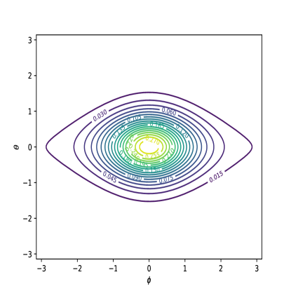
(a)

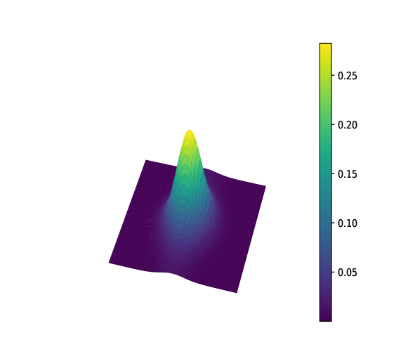
(b)

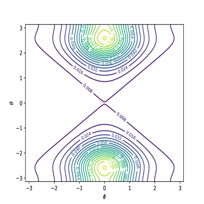
(c)

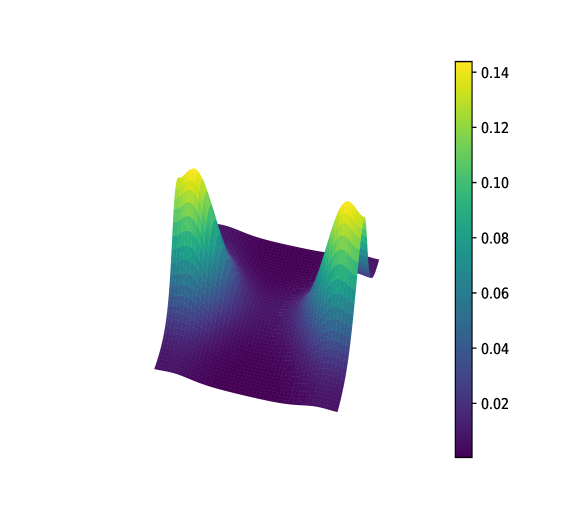
(d)

Figure 2: (a) contour plots and (b) 3D surface plots the proposed bivariate density function provided in Eq. 10 for $(\mu_{1},\mu_{2})=(0,0)$ Ṡimilarly, for $(\mu_{1},\mu_{2})=(0,\pi)$, we present (c) contour plots and (d) 3D surface plots. These visualizations maintain parameters throughout: $(\kappa_{1},\kappa_{2})=(1.5,2.5)$ and $\nu=0.8$. For a better diagrammatic representation, the plots are showed in $[-\pi,\pi)\times[-\pi,\pi)$ instead of $[0,2\pi)\times[0,2\pi).$

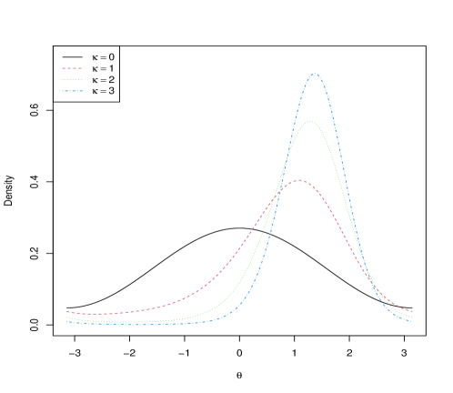
(a)

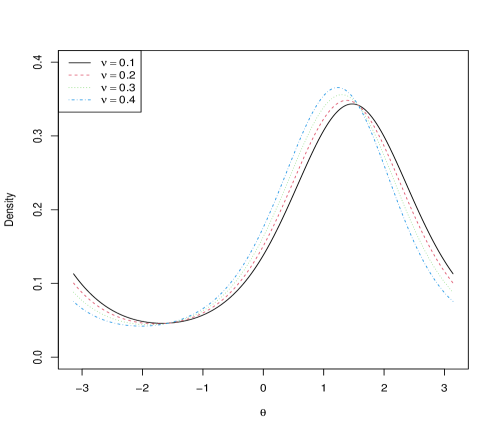
(b)

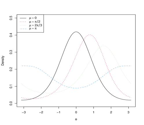
(c)

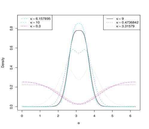
(d)

Figure 3: Density plot of the probability density function provided in Eq. 11 (a) $\mu=\frac{\pi}{2}$ $\nu=0.5$, along with $\kappa=0,1,2,3,4$. (b) $\mu=\frac{\pi}{2}$, $\kappa=1$, along with $\nu=0.1,0.2,0.3,0.4$, (c) $\nu=0.5,~{}~{}\kappa=1$, along with $\mu=0,\frac{\pi}{3},\frac{2\pi}{3},\pi.$ (d) $\mu=\pi,~{}~{}\nu=0.9$, and for different values of $\kappa$. For a better diagrammatic representation, the plots in (a), (b), and (c) are shown in $[-\pi,\pi)$ instead of $[0,2\pi).$

(a)

(b)

(c)

Figure 4: (a) The circular variance plot of the symmetric density in Eq. 29. (b) The plot of the KL divergence $D_{KL}(f_{c},h_{3})$ between proposed and Cardioid density as in Eq. 30 for $\kappa=0,1,\cdots,10$. (c) The plot of the derivative of KL divergence with respect to $\nu\in(0,1)$.

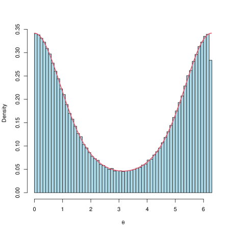
(a)

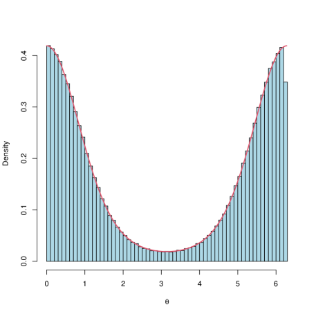
(b)

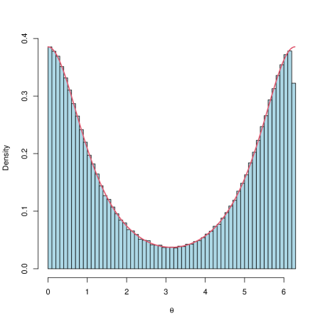
(c)

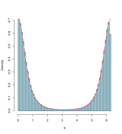
(d)

Figure 5: (a) Histogram of the data from the probability density function $\dfrac{e^{\cos{\theta}}}{2\pi I_{0}(1)}.$ (b) Histogram of the data from the probability density function $\frac{e^{\cos\theta}~{}\left(1+\nu\cos\theta\right)}{2\pi\left[I_{0}(1)+\nu I_{1}(1)\right]}.$ (c) Histogram of the data from the probability density function $\frac{1}{C}f_{wc}(\theta)\left(1+\nu\cos\theta\right)$. (d) Histogram of the data from the probability density function $\frac{1}{C}f_{kj}(\theta)\left(1+\nu\cos\theta\right).$

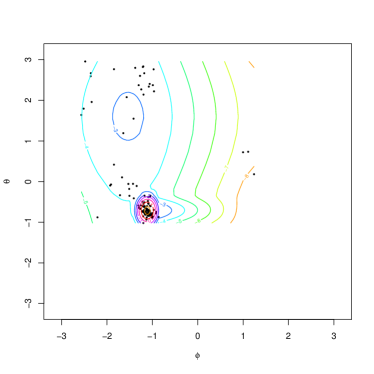
(a)

(b)

(c)

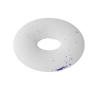
(d)

Figure 6: (a) Showcasing scatter plots and the contour of the logarithm of the probability density function of the torsion angles of the Oxygen Transport protein, chloromet myohemerythrin (1A7D) protein. (b) and (c) represent marginal circular plots for the angles $\theta$ and $\phi$ respectively. (d) depicts a scatter plot of the same on the curved torus. For a better diagrammatic representation, the scatter plot is shown in $[-\pi,\pi)\times[-\pi,\pi)$ instead of $[0,2\pi)\times[0,2\pi).$

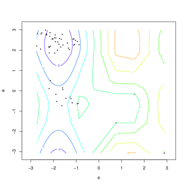
(a)

(b)

(c)

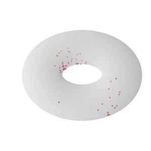
(d)

Figure 7: (a) Showcasing scatter plots and the contour of the logarithm of the probability density function of the torsion angle of the Src-homologous SH3 domain (1SHG). (b) and (c) represent marginal circular plots for the angles $\theta$ and $\phi$ respectively. (d) depicts a scatter plot of the same on the curved torus. For a better diagrammatic representation, the scatter plot is shown in $[-\pi,\pi)\times[-\pi,\pi)$ instead of $[0,2\pi)\times[0,2\pi).$

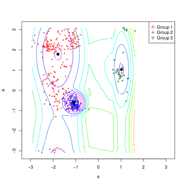
(a)

(b)

(c)

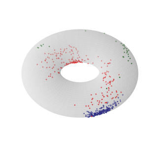
(d)

Figure 8: (a) Showcasing scatter plots and the contour of the logarithm of the probability density function of the torsion angle of the porcine ribonuclease inhibitor protein (2BNH). (b) and (c) represent marginal circular plots for the angles $\theta$ and $\phi$ respectively. (d) depicts a scatter plot of the same on the curved torus. In (a) and (d) the data points are allocated to one of the three probable densities based on their membership values. For a better diagrammatic representation, the scatter plot is shown in $[-\pi,\pi)\times[-\pi,\pi)$ instead of $[0,2\pi)\times[0,2\pi).$

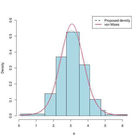
(a)

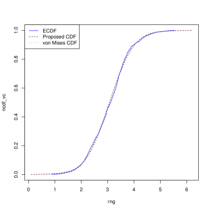
(b)

Figure 9: The figure depicts the wind direction variability at Kolkata, India, over 41 years, specifically for the month of August from the year 1982 to 2023. (a) The histogram of the data of wind directions along with the estimated density obtained through the maximum likelihood estimate (MLE) of the parameters of the general family of distributions with the probability density function according to Eq. 11. Additionally, the two-parameter sub-model, represented by the von Mises density, is displayed as solid lines. (b) The plot of the fitted cumulative distribution functions (CDFs) of the proposed probability density function in Eq. 11 and von Mises distribution along with the empirical cumulative distribution function (ECDF) of the data.

References

- \bibcommenthead
- Ameijeiras-Alonso and Ley [2022] Ameijeiras-Alonso J, Ley C (2022) Sine-skewed toroidal distributions and their application in protein bioinformatics. Biostatistics 23(3):685–704
- Beran [1979] Beran R (1979) Exponential models for directional data. The Annals of Statistics pp 1162–1178
- Best and Fisher [1979] Best D, Fisher NI (1979) Efficient simulation of the von mises distribution. Journal of the Royal Statistical Society: Series C (Applied Statistics) 28(2):152–157
- Bhattacharya and Patrangenaru [2003] Bhattacharya R, Patrangenaru V (2003) Large sample theory of intrinsic and extrinsic sample means on manifolds. The Annals of Statistics 31(1):1–29
- Diaconis et al [2013] Diaconis P, Holmes S, Shahshahani M, et al (2013) Sampling from a manifold. Advances in modern statistical theory and applications: a Festschrift in honor of Morris L Eaton 10:102–125
- Eltzner et al [2018] Eltzner B, Huckemann S, Mardia KV (2018) Torus principal component analysis with applications to rna structure. Ann Appl Stat
- Fisher et al [1993] Fisher NI, Lewis T, Embleton BJ (1993) Statistical analysis of spherical data. Cambridge university press
- Fisher [1953] Fisher RA (1953) Dispersion on a sphere. Proceedings of the Royal Society of London Series A Mathematical and Physical Sciences 217(1130):295–305
- Gao et al [2018] Gao Y, Wang S, Deng M, et al (2018) Raptorx-angle: real-value prediction of protein backbone dihedral angles through a hybrid method of clustering and deep learning. BMC bioinformatics 19:73–84
- Gradshteyn and Ryzhik [2014] Gradshteyn IS, Ryzhik IM (2014) Table of integrals, series, and products. Academic press
- Hamelryck et al [2012] Hamelryck T, Mardia K, Ferkinghoff-Borg J (2012) Bayesian methods in structural bioinformatics. Springer
- Jammalamadaka and Sengupta [2001] Jammalamadaka SR, Sengupta A (2001) Topics in circular statistics, vol 5. world scientific
- Jones and Pewsey [2005] Jones M, Pewsey A (2005) A family of symmetric distributions on the circle. Journal of the American Statistical Association 100(472):1422–1428
- Kagan et al [1973] Kagan AM, Linnik I, Rao CR (1973) Characterization problems in mathematical statistics. (No Title)
- Kato and Jones [2010] Kato S, Jones M (2010) A family of distributions on the circle with links to, and applications arising from, möbius transformation. Journal of the American Statistical Association 105(489):249–262
- Kent et al [2008] Kent JT, Mardia KV, Taylor CC (2008) Modelling strategies for bivariate circular data. In: Proceedings of the Leeds Annual Statistical Research Conference, The Art and Science of Statistical Bioinformatics, Leeds University Press, Leeds, Citeseer, pp 70–73
- Ley and Verdebout [2017] Ley C, Verdebout T (2017) Modern directional statistics. Chapman and Hall/CRC
- Mardia [1975] Mardia KV (1975) Statistics of directional data. Journal of the Royal Statistical Society Series B: Statistical Methodology 37(3):349–371
- Mardia and Jupp [2000] Mardia KV, Jupp PE (2000) Directional statistics, vol 2. Wiley Online Library
- Mardia et al [2007] Mardia KV, Taylor CC, Subramaniam GK (2007) Protein bioinformatics and mixtures of bivariate von mises distributions for angular data. Biometrics 63(2):505–512
- Mardia et al [2008] Mardia KV, Hughes G, Taylor CC, et al (2008) A multivariate von mises distribution with applications to bioinformatics. Canadian Journal of Statistics 36(1):99–109
- McLachlan and Krishnan [2007] McLachlan GJ, Krishnan T (2007) The EM algorithm and extensions. John Wiley & Sons
- Pennec [2006] Pennec X (2006) Intrinsic statistics on riemannian manifolds: Basic tools for geometric measurements. Journal of Mathematical Imaging and Vision 25:127–154
- Rao et al [1973] Rao CR, Rao CR, Statistiker M, et al (1973) Linear statistical inference and its applications, vol 2. Wiley New York
- Rivest [1988] Rivest LP (1988) A distribution for dependent unit vectors. Communications in Statistics-Theory and Methods 17(2):461–483
- Shapovalov et al [2019] Shapovalov M, Vucetic S, Dunbrack Jr RL (2019) A new clustering and nomenclature for beta turns derived from high-resolution protein structures. PLoS computational biology 15(3):e1006844
- Shieh et al [2011] Shieh GS, Zheng S, Johnson RA, et al (2011) Modeling and comparing the organization of circular genomes. Bioinformatics 27(7):912–918
- Singh et al [2002] Singh H, Hnizdo V, Demchuk E (2002) Probabilistic model for two dependent circular variables. Biometrika 89(3):719–723
- Uspensky [1948] Uspensky JV (1948) Theory of equations. (No Title)
- Watson [1983] Watson SG. (1983) Statistics on spheres. Wiley, New York
- Yfantis and Borgman [1982] Yfantis E, Borgman L (1982) An extension of the von mises distribution. Communications in Statistics-Theory and Methods 11(15):1695–1706