First order distinguishability of sparse random graphs
Abstract
We study the problem of distinguishing between two independent samples of a binomial random graph by first order (FO) sentences. Shelah and Spencer proved that, for a constant , obeys FO zero-one law if and only if is irrational. Therefore, for irrational , any fixed FO sentence does not distinguish between with asymptotical probability 1 (w.h.p.) as . We show that the minimum quantifier depth of a FO sentence distinguishing between depends on how closely can be approximated by rationals:
-
•
for all non-Liouville , w.h.p.;
-
•
there are irrational with that grow arbitrarily slowly w.h.p.;
-
•
for all .
The main ingredients in our proofs are a novel randomized algorithm that generates asymmetric strictly balanced graphs as well as a new method to study symmetry groups of randomly perturbed graphs.
1 Introduction
In this paper we focus on the problem of distinguishing between two independent random (simple) graphs by first order (FO) sentences. The vocabulary of FO language of graphs contains the adjacency and the equality relations.
Given two graphs and a FO sentence , we say that distinguishes between and if and , or vice versa. We say that are -distinguishable if there exists a FO sentence with quantifier depth at most that distinguishes between them. Recall that the quantifier depth of a sentence is, roughly speaking, the maximum number of nested quantifiers in (for a formal definition, see [15]). We call the minimum such that are -distinguishable the FO distinguishability, and denote it by . The FO distinguishability was first studied by Spencer and St. John for random sequences [23]. Tight worst-case upper bounds on for deterministic graphs were obtained in [17] by Pikhurko, Veith, and Verbitsky. In this paper we study the FO distinguishability of random graphs. Before stating our results, we discuss some motivation of this problem as well as give an overview of its history.
Distinguishability of random graphs is closely related to zero-one laws, an important phenomenon in finite model theory. We say that a sequence of random graphs satisfies the FO zero-one law if, for every FO sentence , the limiting probability is either or . In other words, either holds with high probability (w.h.p., in what follows) or holds w.h.p. The celebrated theorem of Glebskii, Kogan, Liogon’kii, Talanov [8] and Fagin [7] says that the FO zero-one law holds when , that is, when is distributed uniformly on the set of all labelled graphs on .
The Bridge Theorem (see [22, Theorem 2.5.1 and Theorem 2.3.1]) implies the following relation between zero-one laws and distinguishability: a sequence of random graphs satisfies the FO zero-one law if and only if the respective FO distinguishability is unbounded, i.e. for every ,
In [13] Kim, Pikhurko, Spencer, and Verbitsky proved a more precise estimation: w.h.p. . In [4] Benjamini and the second author of the paper obtained a tight bound: w.h.p. and is concentrated in 3 consecutive points. They also observed that the same result holds true for the number of variables in infinitary logic .
FO distniguishability is also related to the graph isomorphism problem. Note that two finite graphs are isomorphic if and only if there is no FO sentence that distinguishes between them. Since the truth value of a FO sentence of quantifier depth on an -vertex graph can be tested in time [15], upper bounds on the FO distinguishability of graphs imply upper bounds on the time complexity of deciding whether or not the graphs are isomorphic. From this perspective, the problem of distinguishing between two independent copies arises naturally from the average case analysis of the graph isomorphism problem. However, this approach gives a bound that is far from being optimal: it only shows that can be distinguished in quasi-polynomial time w.h.p. A much more efficient algorithm can be obtained by considering FO logic with counting. Indeed, the results of Babai and Kučera [2] and Babai, Erdős, and Selkow [1] (combined with Immerman and Lander’s [10] logical characterization of color refinement) imply that w.h.p. can be defined by a FO sentence with counting quantifiers of quantifier depth 4. This implies a polynomial (actually, even linear) time algorithm that distinguishes between and any non-isomorphic graph w.h.p.
In sparse random graphs, however, the situation is strikingly different. The FO distinguishability can be significantly smaller, and therefore provide much more efficient algorithms for random graphs distinguishing. To state the relevant results, recall the general definition of the binomial random graph: is a random graph on , in which edges between pairs of vertices appear independently with probability . In [21], Shelah and Spencer studied the validity of the FO zero-one law for where is a positive constant.
Theorem 1.1 (S. Shelah, J. Spencer [21]).
Let . Then obeys a FO zero-one law if and only if is irrational.
It follows that, for rational and two independent copies we have with probability bounded away from 0. Furthermore, it can be even derived that, for every , for a certain constant .
For irrational , the asymptotic behavior of is more complicated. Authors of [4] suspected that similar methods to those that were applied for dense random graphs might imply w.h.p. for irrational as well and it was, however, conjectured that actually w.h.p. Our first result shows that this conjecture is true.
For an irrational , we let for two independent . For a sequence of random variables and a sequence of non-zero constants , we write when is stochastically bounded, that is, for every , there exists such that for all .
Theorem 1.2.
Let be irrational. Then .
On the other hand, our second result shows that it is impossible to get a uniform lower bound approaching infinity: may grow arbitrarily slow.
Theorem 1.3.
For every function there exists an irrational and an increasing sequence of positive integers such that w.h.p. (as ) .
We observe that FO distinguishability depends on how well an irrational can be approximated by rational numbers: the better is approximable, the closer the behavior of to the case of rational is. This allows us to prove our third result: in contrast to Theorem 1.3, for almost all , is at least w.h.p. Let us recall that the Liouville–Roth irrationality measure of an irrational number is the infimum (which can be infinite) of the set of all such that at most finitely many integers and satisfy . Due to Roth’s theorem [18], if is algebraic (while for transcendental numbers or — in the latter case is called Liouville number).
Theorem 1.4.
Let and be an irrational number with the Liouville–Roth irrationality measure strictly smaller than . Then w.h.p. . In particular, for almost all irrational (in the Lebesgue measure), w.h.p. .
The second assertion follows from the fact that the set of with irrationality measure strictly bigger than 2 has Lebesgue measure 0 due to Khinchin’s theorem [12]. In particular, the lower bound holds true for all algebraic irrational due to Roth’s theorem. In contrast, in our proof of Theorem 1.3, for a given growing , the corresponding irrational is defined as a suitable Liouville number.
To prove Theorem 1.2 we distinguish from via an existential sentence. The strategy is to find a large family of graphs with the property that w.h.p. there exists which appears as an induced subgraph in but not in . Commonly, in order to verify that a representative of a given isomorphism class appears as an induced subgraph of a random graph, the second moment of the random variable that counts the number of such appearances is computed. When has subgraphs that are at least as dense as itself (i.e., is not strictly balanced), the variance of this random variable becomes large and does not allow to apply a concentration inequality. Moreover, symmetries of negatively affect the expectation of . Therefore, we require to be a large family of asymmetric strictly balanced graphs with a given density.
Our last contribution is the existence of a large family of asymmetric strictly balanced graphs as well as a randomized algorithm for sampling such graphs, that we have used to prove Theorem 1.2. We prove that for every density (this restriction is tight), bounded from above by a constant, there exists a family of strictly balanced asymmetric graphs on of size (see Theorem 2.1 in Section 2). The novel algorithm of sampling random balanced graphs that are w.h.p. asymmetric that we present in Section 2.1 is inspired by the proof of Ruciński and Vince [20] of the existence of a strictly balanced graph for every fixed density . In order to prove that the random balanced graph is asymmetric w.h.p., we develop a new approach for proving asymmetry of randomly perturbed graphs, based on the concept of alternating cycles, i.e. cycles whose edges alternate between the edges of a fixed deterministic graph and the random edges. We believe that these results are interesting in their own right — strictly balanced graphs and their generalizations (as well as their automorphisms) naturally arise in different contexts in random graphs theory, see, e.g., [9, 19, 20] and [11, Chapter 3].
The paper is organized as follows. In Section 2 we define the random balanced graph, study its properties, and then show that it can be used to prove the existence of a large family of strictly balanced asymmetric graphs. The crucial property of the random balanced graph — asymmetry — is proved in Section 6. The existence of a large family of strictly balanced asymmetric graphs is used in Section 3 to prove Theorem 1.2. Sections 4 and 5 are devoted to proofs of Theorems 1.3 and 1.4 respectively. Note that the proof of Theorem 1.4 requires the random balanced graph and its asymmetry as well.
Notations and conventions
Throughout the text, we often maintain a convention of denoting random variables in boldface letters.
For a graph , we denote by and the number of vertices and edges in respectively. In addition, is the minimum degree of and is the maximum degree of . For a set of vertices , let denote the subgraph of induced by .
We will sometimes need to work with multigraphs. We often use asterisks to distinguish multigraphs from simple graphs, unless the distinction is clear from the context. Recall that a multigraph is a pair where is a set of vertices and is a multiset of edges (loops are allowed). is the number of edges counted with multiplicities. Given two multisets , we define their sum as the multiset with the property for every , where denotes the multiplicity of in . For two multigraphs on the same vertex set , we define their sum as . Note that . When we talk about (multi)graphs on vertices, we always refer to labelled graphs with vertex set .
We use the asymptotic notations for and for .
Note that the symbol is also used to denote sampling from a distribution, e.g. . The two meanings of the symbol are distinguished by the context.
2 The random balanced graph
In this section we introduce a random graph model, denoted , which we call the random balanced graph (with vertices and edges). We then use it to generate a large family of asymmetric, strictly balanced graphs on with a given density. This will be the key ingredient in our proof of Theorem 1.2 and Theorem 1.3
Recall that a graph is balanced if for every subgraph , where is the density of . Furthermore, is strictly balanced if for every proper subgraph . Also recall that a graph is asymmetric if its group of automorphisms is trivial. The same definitions apply for multigraphs.
In Sections 3 and 4 we will be interested in the case where the density approaches as . Here we consider a more general setting of a bounded density. The main goal of this section is to prove the following theorem.
Theorem 2.1.
Fix a constant and let satisfy . Then, for every even positive integer , there exists a family of strictly balanced and asymmetric graphs on and edges such that .
Remark 2.2.
It makes sense to consider only connected graphs since a disconnected graph is not strictly balanced, and so should be at least . On the other hand, any tree is strictly balanced. Up to isomorphism, there is only one connected graph with edges which is strictly balanced — a cycle , though it is not asymmetric. Finally, every strictly balanced graph with edges is either a cycle with a path between its two vertices, or two cycles joined by a path. Clearly, both graphs are not asymmetric. Thus, the condition is necessary unless the graph is a tree.
Remark 2.3.
Although we believe that the assertion of Theorem 2.1 is true for odd as well, we state it in this weaker form since an adaptation of our approach to odd requires a more complicated case-analysis to prove strict balancedness. As for our purposes it is enough to consider even , we omit these technical complications.
In Subsection 2.1 we define , in Subsection 2.2 we study its properties, and in Subsection 2.3 we complete the proof of Theorem 2.1.
2.1 Definition
From now on fix and assume that is even and , where is a constant. We begin with a definition of the random balanced multigraph . It is inspired by Ruciński and Vince’s construction of a strictly balanced graph [20]. Write where and are integers. is defined as the sum of three different (multi)graphs, which we call components: the regular component with edges, the Hamiltonian component with edges and the balancing component with edges.
Let be a cycle of order ; write it as . For a given , define the following set of almost equidistributed vertices around :
| (1) |
Note that indeed . In addition, for any sequence of consecutive vertices in , less than of them belong to . Indeed, a sequence of vertices (with indices taken modulo ) has vertices from , and this is less than . This property shows that the vertices of are distributed almost equally, which is useful for proving balancedness.
Definition 2.4.
The random balanced multigraph with vertices and edges is defined as follows.
-
•
Let be a uniformly distributed -regular (simple) graph on .111We refer to [11, Chapter 9] as an introduction to random regular graphs.
-
•
Let be a uniformly random Hamilton cycle, independent of .
-
•
Let be defined as follows. For every choose a random vertex , such that these vertices are chosen independently of and , and are uniformly distributed over all possible sequences of distinct vertices. Now define . We regard as a multiset: edges may have multiplicity and loops are allowed. Thus may be a multigraph.
Finally, define . Edges of are called regular, edges of are called Hamiltonian, and edges of are called balancing.
Remark 2.5.
The requirement that the vertices are all distinct is introduced in order to restrict the maximum degree of . Indeed, note that is a -regular multigraph, and that degrees in are , or . Therefore
| (2) |
Remark 2.6.
Let denote the number of possible values of . By definition, , where is the number of -regular graphs on vertices (see [11], Corollary 9.8); is the number of cycles on ; is the number of sequences of distinct vertices. Note that is uniformly distributed over all possible values. However, itself is not uniformly distributed. This is because different multigraphs may be represented as a sum in a different number of ways.
Definition 2.7.
The random balanced graph is defined as a random (simple) graph whose distribution is the distribution of conditioned on being simple.
Remark 2.8.
Let be the number of possible values of such that is a simple graph. Conditioning by the event that is simple, is uniformly distributed over all possible values.
2.2 Properties
In this subsection we list several important properties of . The main three properties are strict balancedness (Proposition 2.9), a bound on the probability that contains a given set of edges (Proposition 2.13), and asymmetry (Theorem 2.15).
Proposition 2.9.
Suppose is a graph such that . Then is strictly balanced.
Although the proof of Proposition 2.9 resembles the proof of Ruciński and Vince that the graphs that they construct in [20] are strictly balanced, below we present the full proof for completeness.
Proof.
We actually prove a stronger statement: if then is strictly balanced.
Consider a possible value of of and let . We shall prove that is strictly balanced. That is, we show that every proper sub-multigraph satisfies
We now follow a sequence of reductions.
First, we claim that it suffices to prove strict balancedness of . Indeed, suppose that is strictly balanced. Consider a set and denote , and . Since is strictly balanced,
Now, is obtained from by adding some edges of the -regular graph , which increases the degree of each vertex by at most . Therefore at most edges are added. Overall
which proves strict balancedness of .
Second, we claim that it suffices to prove strict balancedness of , which is obtained from by replacing its balancing edges with loops: each edge is replaced with a loop at . Indeed, suppose that is strictly balanced. Consider a set and denote , and . It is easy to see that . From strict balancedness of ,
which proves strict balancedness of .
Third, we claim that to prove strict balancedness of , it suffices to check only which are segments of the Hamiltonian component ; that is, sequences of consecutive vertices on the cycle. Indeed, assume that we have verified strict balancedness for segments. Consider a set and denote and . Notice that can be written as the union of mutually disjoint segments with no Hamiltonian edge between them. Let denote the number of vertices and edges in . From the assumption, for every . Then
which proves strict balancedness.
Finally, it remains to check strict balancedness of for segments. Take any segment with vertices. The subgraph contains Hamiltonian edges and less than loops (since the loops are almost equidistributed). Therefore
That finishes the proof. ∎
Proposition 2.10.
There exists a positive constant such that .
Remark 2.11.
Proof of Proposition 2.10.
Let be the event that is simple. Then , where
-
1.
is the event that and do not share common edges.
-
2.
is the event that does not contain loops or edges with multiplicity and does not share edges with or with .
We write and prove that there are positive constants such that , .
is equal to the probability that the random -regular graph does not contain any edges of a given Hamilton cycle. When it is clearly , so assume . We apply [16, Theorem 1.1], which bounds the probability that a random graph with specified degrees does not contain any edges of a given subgraph. For the special case of regular graphs it yields the following statement.
Theorem 2.12 (B. McKay [16]).
Let be an integer and let be a graph on vertex set and maximum degree . For every even let denote the number of labelled -regular graphs on that do not contain any edge of . Then
Here is the number of edges in a -regular graph on vertices.
In our case, let (which is a constant) and let be a Hamiltonian cycle, so and . Also let denote the empty graph (on vertices), so is the number of labelled -regular graphs. Then
Hence is bounded from below by a positive constant.
Now let us bound . We fix values and such that holds, and prove the existence of a constant (independent of ) such that
Let (the labeling may be chosen arbitrarily) be the set of equidistributed vertices around . Since holds, is a simple -regular graph. The sequence of values is drawn uniformly from all the sequences of distinct vertices. We provide a lower bound on the number of choices which satisfy .
Let us sequentially choose the values , making sure that is satisfied at every step. When we get to , there are at least possible choices which assure that is still satisfied. We deduce
Here follows from , follows from , and holds since decreases as a function of . ∎
Proposition 2.13.
There exists a positive constant such that, for every set , we have .
Proof.
The idea is to partition into three disjoint sets and separately bound the probability that they are subsets of . It will be simpler to work with , and for that we will rely on Proposition 2.10.
Formally, fix and let be the set of triplets which form a partition of . Note that . For every let denote the event that in we have , , . Then, from Proposition 2.10,
We will now prove that there exists a constant such that for every . Then, taking finishes the proof.
So, let us fix a partition of . Let and similarly define .
Step 1. We apply the following proposition from [5].
Proposition 2.14 ([5], Equation (2)).
Fix a constant and let be a random -regular graph on vertices. Then there exists a constant (depending on but not on ) such that, for every set , .
In our case, it follows that there exists a positive constant such that .
Step 2. Let us bound . Recall that is the set of edges of a random Hamilton cycle. If is not contained in any Hamilton cycle, this probability is trivially , so assume that it is not the case.
If , then is already the set of edges of a Hamilton cycle, and then .
If , then the graph has exactly connected components, all of them are either paths or isolated vertices (which are not considered as paths for now). Let be the number of paths. Then the number of Hamilton cycles containing equals . Therefore
Note that the last bound also holds when .
Step 3. Finally, let us bound . We shall prove that for every possible value of ,
That will prove
Fix a value . It determines the set of equidistributed vertices . Again, we arbitrarily enumerate it: . Recall that is defined as the (multi)set of edges of the form , where are drawn uniformly from all possible sequences of distinct vertices. The number of ways to choose the vertices such that holds is at most . Indeed, there are at most ways to choose a direction for every edge of and at most ways to choose the remaining . Overall,
In conclusion, the three steps and the independence between the different components of show that indeed there exists a constant such that . That finishes the proof. ∎
Finally, we address the asymmetry of .
Theorem 2.15.
is asymmetric w.h.p.
Proof.
We consider two separate cases and .
Dense case: . In this case we follow an argument due to Bollobás [5], which proves asymmetry of the random regular graph with fixed. This argument directly generalizes to the following result.
Theorem 2.16 (Bollobás [5]).
Fix an integer constant . Let be a sequence of random graphs with and . Assume that there exists a constant such that for every . Then is asymmetric w.h.p.
Equation (2) and Proposition 2.13 show that the random balanced graph satisfies properties 2 and 3. When it also satisfies property 1, and therefore it is asymmetric w.h.p.
Sparse case: . In this case and Bollobás’s argument does not apply. Instead, we develop an entirely different approach for proving asymmetry, generally applicable to randomly perturbed cycles. Indeed, in the sparse case, the regular component vanishes and . That is, is a Hamilton cycle with additional randomly scattered edges. Our approach is based on the observation that non-trivial automorphisms give rise to certain configurations which are very rare in the sparse case. A key concept in the proof is that of an alternating cycle: a cycle which alternates between Hamiltonian edges and balancing edges. Since this proof may be of its own interest and since it is long enough to interrupt the flow of the paper, we present it in the separate Section 6. ∎
2.3 The family
We are now ready to prove Theorem 2.1. Given which satisfies , define as the set of all asymmetric graphs which are possible values of . That is,
is indeed a family of strictly balanced and asymmetric graphs with vertices and edges (by the definition and from Proposition 2.9). Note that it is closed under isomorphism (since so is the family of all possible values of ).
It remains to prove that . We start with an estimation of . Recall that
From Proposition 2.10 we have . Combining that with Theorem 2.15, we deduce that the number of possible such that is an asymmetric (simple) graph is at most . The only remaining issue is that we may overcount graphs: different values may have the same sum. To handle this, the following simple lemma bounds the number of ways to express a given (simple) graph as . We allow very coarse estimations since we only care that the bound is exponential.
Claim 2.17.
There is a function such that, for every graph , the number of possible values of such that is at most .
Proof.
From (2) we know that . Therefore is a trivial (and very coarse) bound on the number of Hamilton cycles in . The Hamiltonian component must be one of them.
Now fix , which also fixes the set . For every , must be its neighbor in and can therefore be chosen in at most ways. So the number of choices for is at most .
The values uniquely determine (as the graph with all the remaining edges). Overall, the number of choices is at most
where we used the inequalities and . That finishes the proof. ∎
3 The general upper bound
In this section we prove Theorem 1.2. Let us fix an irrational and a function , and let be independent. We prove that there exists a purely existential FO-sentence , of quantifier depth at most , that distinguishes between w.h.p. To do that, it is sufficient to find a family of graphs on where is even and satisfies the following two properties:
- (A)
-
W.h.p., contains an induced subgraph which is isomorphic to some .
- (B)
-
For any specific graph , w.h.p. does not contain an induced subgraph isomorphic to .
Indeed, suppose we have found with these properties. Let be the minimum graph from (with respect to some arbitrary ordering) such that contains an induced subgraph isomorphic to . From (A), such a graph exists w.h.p. Now let be a FO-sentence expressing the property of containing an induced subgraph isomorphic to , with quantifier depth at most . From (B), it distinguishes between w.h.p.
Our approach is to define as a set of typical graphs from the family from Theorem 2.1, with around . More precisely, we set : the additional makes the subgraphs dense enough to assure Property (B). We get Property (A) in the usual way using Chebyshev’s inequality. To make it work, we need asymmetry and strict balancedness that are provided by Theorem 2.1. For technical reasons, we need to further refine the latter property and make sure that our family comprises graphs that are enhancely balanced, i.e. small subgraphs of have density slightly below . We will make use of the following proposition.
Proposition 3.1 (Enhanced Balancedness).
Consider with even and . Then there exist positive constants (depending only on ) such that the following holds. W.h.p., for every subgraph of with , we have .
The proof of Proposition 3.1 is postponed to Subsection 3.2. In Subsection 3.1 we use it to construct a family with Properties (A) and (B) and thus complete the proof of Theorem 1.2.
3.1 A suitable family of subgraphs
Let be the family of graphs from Theorem 2.1 with , Without loss of generality we may assume that is even. We define as the family of graphs which additionally satisfy the enhanced balancedness property from Proposition 3.1. Like , the family is closed under isomorphism. Moreover, from Theorem 2.1, Proposition 3.1, and Claim 2.17, we have the following bound on .
Claim 3.2.
Proof.
Lemma 3.3.
satisfies Property (B).
Proof.
Fix and let be the number of induced copies of in . Then
since and . From the definition of we have , so overall . From Markov’s inequality, . ∎
Lemma 3.4.
satisfies property (A).
Proof.
Let count the number of induced subgraphs with . We need to prove . From Chebyshev’s inequality, it suffices to prove Write , where the sum is over all subgraphs of the complete graph with . The expected value is
The variance is
| (3) |
We decompose the sum in (3) by considering different possible intersection patterns of . For every non-negative integers let denote the sum in (3), but only over the pairs which share exactly common vertices and common edges. Then . When , the indicators are independent and the corresponding summand is . Taking enhanced balancedness into account, we may therefore sum over the set of pairs such that , and, moreover, whenever . Each can be written as follows:
Here denotes the number of possible choices of a pair of induced subgraphs on two given sets of vertices with common vertices, such that and they share exactly edges. Simple estimations yield
| (4) |
The following claim bounds the term .
Claim 3.5.
For every , , where is the constant from Proposition 2.13, and the term does not depend on .
Proof.
Let us fix two sets of vertices with and having . We need to bound , the number of pairs such that each is a graph on with , , and the common induced subgraph contains exactly edges.
First choose on such that contains exactly edges. The number of choices is trivially bounded by . Now, given , we must choose on which contains a given set of edges. The number of choices is bounded by the number of graphs from that contain the same set of edges which is, due to Proposition 2.13, at most , where is again the number of possible values such that is simple. By Claim 3.2, . Therefore
∎
We now return to the proof of Lemma 3.4. It suffices to prove that the right-hand side in (4) is (uniformly), since the number of summands is . We have
Notice that the last expression is monotonically increasing with respect to . Therefore we may bound it for every only with , defined as the maximal such that . Note that , so
| (5) |
We bound (5) separately for small and for large . Intuitively, for small subgraphs the enhanced balancedness property promises that is sufficiently small, while for large subgraphs it is which becomes small.
Small Subgraphs. In this case we assume where . By definition of ,
Of course, this implies , so enhanced balancedness applies: and therefore .
As for , we use the simple bound
Without loss of generality, we may assume , so and
Overall, uniformly. In particular it is .
Large Subgraphs. Now assume . In this case we only know , so
As for , we have
where is a positive constant. Combining both bounds,
for some constant . Note that
Again, without loss of generality we may assume , so
Overall, which is again . We have therefore completed the proof of Lemma 3.4. ∎
3.2 Proof of Proposition 3.1
It remains to prove Proposition 3.1 about enhanced balancedness. We have with and . Write where is an integer and . Then where .
Definition 3.6.
Let be a random balanced (simple) graph. Let be obtained by deleting the regular edges from . Let be obtained from by replacing every balancing edge with a loop at . That is, is simply the Hamilton cycle with a loop at every vertex of .
Definition 3.7.
For a given set of vertices , its segment decomposition is , where are mutually disjoint segments of the Hamiltonian component with no Hamiltonian edge between them.
We shall use the following technical claim.
Claim 3.8.
For every positive integer there exists a positive constant such that the following holds. Let be a set of vertices and let . If the segment decomposition of contains a segment of length at most , then
Proof.
Fix a positive integer . Define
where the minimum is over all integers with and . This is a minimum over a finite, fixed set and thus is a positive constant. Note that by definition.
First let be a segment with vertices. Let be the number of edges in the induced subgraph . Recall that is strictly balanced and its density is . Also recall that , therefore
Since is a constant, for a sufficiently large , the inequality implies (whenever ). In turn, implies by the definition of .
Now let be a segment of any length. Again, let be its number of vertices and let be the number of edges in . In this case we can only use strict balancedness to claim that
Finally, let be an arbitrary set of vertices. Let be the segment decomposition. By definition, contains no edges between any pair . Let denote the number of vertices and edges in and let denote the number of vertices and edges in . If at least one of the segments is of length ,
That finishes the proof of the claim. ∎
Let us now finish the proof of Proposition 3.1. Set and let be the corresponding constant from Claim 3.8. We prove Proposition 3.1 for and . These choices will be justified soon; for now, notice that .
Let be a subset with and let . We begin by identifying several cases in which the desired inequality holds. The lost edges of are the balancing edges with and .
Fact 1. Suppose that has a lost edge. Then, from Claim 3.8,
Here, the first inequality follows from that fact that is obtained from be adding some edges of the -regular graph , and therefore , while is obtained from by replacing its balancing edges with loops, and adding a loop for every lost edge of .
Fact 2. Suppose that the segment decomposition of contains a segment of length at most . Then, from Claim 3.8,
Fact 3. Denote . Then . In particular, if , we again have
These three facts show that in order to finish the proof, it is sufficient to prove the following statement. W.h.p., for every subset with , if it is composed only of segments of length at least and satisfies , then it has a lost edge.
For with and , the probability that it has no lost edges is precisely in , and in (see Proposition 2.10). Assuming ,
Now consider the number of subsets with vertices which are composed only of segments of length at least . It is bounded by the number of subsets which are composed of at most segments, which is . By the union bound, the probability that no relevant has a lost edge is
| (6) |
It remains to show that the last sum is . The standard bound yields
The last inequality follows from the inequality (applied for ) and the fact that (which follows from the definition of ).
We divide the above sum into two: the sum over and the sum over . First,
Finally,
since by the definition of . That finishes the proof.
4 Low upper bounds for well-approximable
In this section we prove Theorem 1.3. Recall that for a given function (which can grow arbitrarily slowly), our goal is to find an irrational and an increasing sequence of positive integers such that w.h.p. two independent copies can be distinguished by a FO sentence of quantifier depth at most . For the rest of this section, let us denote these copies by for notational convenience.
The construction of a suitable irrational is explicit. The idea is to take which is very well-approximable by rational numbers; the slower grows, the better the approximations must be. Then, along a subsequence (which is determined by the sequence of approximations of ), distinguishing between is essentially the same as in the rational case. This idea naturally leads to the theory of Diophantine approximations, and specifically to the concept of Liouville numbers.
4.1 Diophantine approximations
The theory of Diophantine approximations studies approximations of real numbers by rational numbers. One of its well-known applications is the celebrated Liouville’s theorem, which was used to establish the existence of transcendental numbers for the first time. A Liouville number is an irrational number such that for every , there exists a rational with such that . Liouville’s theorem implies that Liouville numbers are transcendental. For a comprehesive survey on this subject, see [3]. Liouville provided as an example of a Liouville number. For our purposes, however, we will need Liouville numbers which are much better approximated. From now on, when we write a rational number as , we always assume that and that .
Definition 4.1.
Let be a decreasing function. An irrational number is called -approximable if, for infinitely many rational numbers , .
Lemma 4.2.
For every descreasing function there exists an irrational which is -approximable.
Proof.
First notice that if satisfy and is -approximable, then is also -approximable. Therefore, without loss of generality, we may assume . Recursively define a sequence of natural numbers as follows: , . Now define . Without loss of generality, we may assume that is decreasing sufficiently fast such that is a strictly increasing sequence. In that case, is an irrational number because its binary expansion is aperiodic. For every , consider the rational approximation of , which can be written as for and . Then
∎
As in Section 3, we distinguish between two independent through their subgraphs; however, some details are different. First, here we count (all) subgraphs instead of induced subgraphs. We consider subgraphs with densities that approximate well so that the variables counting copies of these subgraphs asymptotically behave like independent Poisson variables (as in the case of a rational ). In particular, a single subgraph suffices to distinguish from with positive probability. To distinguish w.h.p., we shall consider different subgraphs and approximate their joint distribution.
4.2 Asymptotic Poisson behavior
We now return to the proof of Theorem 1.3. Let be the inverse of , that is, . Without loss of generality, (1) is non-decreasing and surjective, (2) , (3) strictly decreases with . Let be an irrational number which is -approximable for ; its existence is guaranteed by Lemma 4.2. Let be the suitable sequences from the proof of the lemma: increasing sequences of natural numbers such that, for every , are coprime and
Write and and also define . Our first assumption on implies that . From now on we focus on the subsequence , so the underlying parameter is now . For convenience, we often omit the dependency on from the notation; all quantities implicitly depend on unless we explicitly state that they are fixed.
Let be the set of graphs from Theorem 2.1. Recall that is a family of asymmetric graphs which is closed under isomorphism. Therefore it contains isomorphism classes. From the asymptotic estimation on given in Theorem 2.1 it follows that . Let be representatives of the isomorphism classes. For every let count copies of in and let count copies of in . In order to complete the proof, it is sufficient to prove the following.
Proposition 4.3.
W.h.p. as , there exists such that either and , or and .
We postpone the proof of Proposition 4.3 to the very end of this section since first we have to prove several auxiliary assertions.
First of all, let us show that asymptotically behave like independent Poisson random variables. We do that using the method of moments (see [11], Subsection 6.1). Note that the method of moments applies only when the number of variables is fixed, so we start by fixing some and considering only the first variables (assuming that the underlying is sufficiently large such that ).
Recall that for summations of Bernoulli random variables, it is easier to deal with factorial moments rather than usual moments. For a random variable , its -th factorial moment is , where . For a -tuple of variables , its -th joint factorial moment equals to
Lemma 4.4.
Fix and non-negative integers . Then, with the above definitions, we have
Proof.
Let us denote and . Then, by decomposing into a sum of indicator random variables, we can write
| (7) |
where the sum is over all -tuples
| (8) |
such that are distinct copies of in the complete graph for every . Let us divide the sum in the right hand side of (7) into two parts: where is the sum over the -tuples which do not share any vertices with each other, and is the remaining part of the sum.
We first estimate . Since are asymmetric, it is easy to see that
By the definition of , we have , which can also be written as . Since decreases and , we get . Therefore,
It remains to prove . Let be the family of all graphs (up to isomorphism) which are the result of a union of distinct copies of for every , with at least one shared vertex. For every , let be the sum from (7) but only over the -tuples whose union is isomorphic to . Then .
Fix . Let denote the number of -tuples as in (8) such that are distinct copies of and . Then
Since for all , then following the usual argument that is used to prove that the union of intersecting strictly balanced graphs with the same density has higher density, we derive the following claim.
Claim 4.5.
For every , the inequality holds for any constant .
Proof.
For a graph we define . We begin with a few simple observations.
Observation 1. If is isomorphic to one of , we have . This is because by definition.
Observation 2. For every two graphs ,
Observation 3. Suppose is isomorphic to one of and let be a proper subgraph with vertices and edges. Since is strictly balanced, we have Furthermore,
Denote (which is positive). Then
Since , we get that for any constant (of course, this becomes true when the underlying is sufficiently large).
With these observations, we now prove Claim 4.5 by induction on .
We start with the induction base . Suppose where are both from and share a vertex. Then
is isomorphic to some proper subgraph of , therefore
Now, suppose the statement is true for and prove it for . Let be the union of certain copies of graphs from such that, without loss of generality, share a vertex. Let . Then
is isomorphic to a subgraph of (not necessarily proper this time). If then . If then the third observation shows that , but and therefore . From the inductive assumption, in both cases and that finishes the proof.
∎
From Claim 4.5, we can write for any constant . Finally, is trivially bounded by . Overall
where the last estimation follows from the assumption . That finishes the proof. ∎
Corollary 4.6.
Fix ; then converges in distribution to where are independent.
We are now ready to prove Proposition 4.3.
5 A lower bound for almost every
In this section we prove Theorem 1.4. That is, we fix and an irrational with Liouville-Roth irrationality measure strictly smaller than and show that w.h.p. there is no FO-sentence of quantifier depth less than distinguishing between two independent copies . To prove this, we present a generalization of Theorem 1.1. The proof of the zero-one law for irrational relies on the existence of a winning strategy of the second player in the Ehrenfeucht-Fraïssé game with a bounded number of rounds. We show that a similar winning strategy can be used by the second player when the number of rounds grows with sufficiently slowly, provided that is not too well-approximable by rational numbers.
From now on we fix with Liouville-Roth irrationality measure strictly smaller than . Let be such that is not -approximable, that is, for all but finitely many .
5.1 The Ehrenfeucht-Fraïssé game
We begin with a brief overview of the Ehrenfeucht-Fraïssé game (see Chapter 2 of [22] for a more detailed exposition). Given two graphs (with disjoint vertex sets) and , the Ehrenfeucht-Fraïssé game is described as follows. The game has two players, called Spoiler and Duplicator, and consists of rounds. The graphs are the “board” on which the players make their moves. In the -th round, Spoiler selects a vertex in either graph (to his choice) and marks it . Duplicator responds by selecting a vertex in the other graph, and also marks it . At the end of the game, let be the vertices of marked (regardless of who marked them) and let be the vertices of marked . Duplicator wins if there exists a partial isomorphism from to which maps to for every . That is, Duplicator wins if and for every . The importance of the Ehrenfeucht-Fraïssé game comes from the following key result, relating it to the FO distinguishability.
Theorem 5.1 (Ehrenfeucht [6]).
Let be two graphs and let . Then Duplicator has a winning strategy in .
From this result we see that, in order to prove Theorem 1.4, it suffices to prove that w.h.p. Duplicator has a winning strategy in . Below, we show that the winning strategy of Duplicator introduced by Shelah and Spencer (look-ahead strategy) can be used for rounds as well. We present the strategy and explain the main properties of the random graph that allow Duplicator to use it. Proofs of these properties are postponed to Appendix B since they resemble the proof in the case of constant number of rounds. For the original argument, we refer to [22, Chapters 4–6].
5.2 Extensions and the closure
The look-ahead strategy is based on the validity of certain -sentences known as extension statements. The original argument considers statements with a constant number of variables, but now we allow it to grow with . We begin by generalizing the concept of safe extensions and their main feature: they w.h.p. exist over any tuple of root vertices.
A rooted graph is a graph with a designated subset of root vertices . It is denoted by the pair . We allow but not . Rooted graphs can be used to define graph extensions as follows. Let be a rooted graph and label its vertices where are the roots and are the non-roots. Let be any graph and let be an -tuple of distinct vertices of . An -extension of is defined as a -tuple of distinct vertices of such that: (1) in whenever in ; (2) in whenever in . Note that this definition does not consider edges between root vertices, and allows for additional edges except those specified by . Also note that the definition implicitly assumes an underlying labeling of the vertices of . From now on, whenever a rooted graph is introduced, we always implicitly assume that it is equipped with a predetermined labeling.
A rooted graph has three parameters: the number of root vertices , the number of non-root vertices , and the number of edges (excluding edges between root vertices) . We call the type of the rooted graph. The following definitions depend on the fixed , and are designed to be used in studying extensions in .
Definition 5.2.
Let be a rooted graph of type . If we say that is sparse. If we say that is dense.
Since is irrational, every rooted graph is either sparse or dense.
Definition 5.3.
Let be a rooted graph and let . We call a subextension of . We also call a nailextension of .
Note that is always a subextension and a nailextension of itself.
Definition 5.4.
A rooted graph is called safe if all its subextensions are sparse, and rigid if all its nailextensions are dense.
The next step is to generalize the Finite Closure Theorem [22, Theorem 4.3.2] (we rename it as Finite Closure Lemma). We first recall the definition of the -closure of a set of vertices.
Definition 5.5.
For a graph , a subset , and , we define the -closure of , denoted , as follows: is the minimum set of vertices which contains and is closed with respect to taking rigid extensions with at most non-roots.
Now consider In what follows, we deal with rooted graphs of type with roots. Importantly, we now allow to depend on , so , and . As we shall see, the original argument can be stretched up to which grow as . Thus, we denote and always assume that .
Lemma 5.6 (Bounded Closure Lemma).
There exists a constant such that w.h.p. in , for every , the -closure of every -tuple has size at most .
Finally, we generalize [22, Theorem 5.3.1] about the existence of generic extensions.
Definition 5.7.
Let be a rooted graph of type with roots. Fix a non-negative integer . For tuples and , we say that an -extension of is -generic if: (1) There are no additional edges between the vertices of or from to other than those specified by . (2) If any with forms a rigid extension over , then there are no edges between and .
Lemma 5.8.
W.h.p. in , for every safe rooted graph with roots and non-roots and for every , we have that every -tuple of vertices has a -generic -extension .
5.3 Look-ahead strategy
The look-ahead strategy guarantees a win for Duplicator in the Ehrenfeucht-Fraïssé game. The previous results allow us to apply the look-ahead strategy in where are independent. Let us recall relevant definitions.
Definition 5.9.
Let be a tuple of vertices in a graph and let be a tuple of vertices in a graph . Also let . We say that the -closures and are isomorphic, and write , if there exists a graph isomorphism from to that sends to for every . The -type of a tuple is the isomorphism class of with fixed .
Definition 5.10.
Given a sequence of nonnegative integers , a look-ahead -strategy for Duplicator in is a strategy that satisfies the following condition. For every , when there are rounds remaining in the game, the -types of the already marked vertices are the same in both graphs.
The following lemma (see [22, Chapter 6]) summarizes the deterministic part of the original argument about the existence of a look-ahead strategy.
Lemma 5.11 ([22]).
Let be two graphs and let be non-negative integers. Let and be two tuples with the same -type. Assume that is an integer such that -closure of any -tuple in has at most non-roots (so at most vertices overall). Also assume that for every rooted graph with roots and non-roots, every -tuple in has a -generic -extension. Then, for every (representing Spoiler’s move) there exists such that and have the same -type.
We can now prove the existence of a look-ahead strategy in , and thus complete the proof of Theorem 1.4.
Proof of Theorem 1.4.
Let be independent and set . Let be the event that the conclusions of Bounded Closure Lemma and Theorem 5.8 hold in both and . Then . We show that, given the event , Duplicator has a winning strategy in .
Construct a sequence inductively as follows: , and given , we take such that the -closure of any -tuple in both and has at most non-roots. Note that these are the conditions from Lemma 5.11 with , and . From the Bounded Closure Lemma, a suitable exists, and can be taken to be where is a constant (note that it also promises as long as we take ). From Theorem 5.8 (with replaced by ), for every rooted graph with roots and non-roots and for every , we have that in both and , every -tuple has a -generic -extension.
Note that if then the assumptions of Lemma 5.11 apply with as above. Indeed, we have and , so and , and so for every rooted graph with roots and non-roots, every -tuple has a -generic -extension. We deduce that Duplicator can follow a look-ahead -strategy, provided that . To show that we consider the recurrence relation defining . We have , and for every ,
where . We deduce where and , implying . Overall we have
where we used the assumption . That finishes the proof. ∎
6 Asymmetry: sparse case
In this section we prove the asymmetry of the random balanced graph for the sparse case , thus completing the proof of Theorem 2.15.
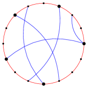
Fix with and let . Write where . The regular component of is therefore empty and . That is, is a random -cycle with additional random balancing edges. Note that the lower bound cannot be improved: a cycle with one additional edge has a single non-trivial isomorphism.
We first expose the edges of . Due to symmetry, it is sufficient to prove that w.h.p. is asymmetric subject to . Let be the set of almost equidistributed vertices. The only random component is therefore the endpoints , which determine the balancing edges .
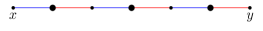
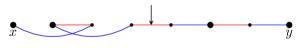
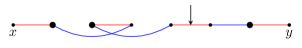
For a more convenient description of the proof, let us color the Hamiltonian edges in red and the balancing edges in blue. Since we are working with the simple graph , every edge is assigned with exactly one color. The red edges are deterministic while the blue edges are random; see Figure 1.
The rest of the section is organized as follows. In Section 6.1 we list several configurations which occur in with probability . A key concept in the proof is that of an alternating cycle, which is a cycle with edges of alternating colors. We show that w.h.p. contains no two large alternating cycles with equal degree sequences, no two small alternating cycles which are connected by an alternating path, no small alternating cycles with additional internal edges, and does not contain some other rare configurations. In Section 6.2 we show that these configurations naturally arise from symmetries of , and thus prove that is asymmetric w.h.p.
6.1 Rare configurations
Definition 6.1.
An alternating walk in is a walk such that colors of the edges alternate between red and blue. An alternating path is an alternating walk without repeated vertices. An alternating cycle is an alternating walk with and no other repetitions. Note that an odd alternating cycle contains two adjacent edges of the same color.
Let us call labeled cycles equipotent in , if, for every , vertices and have equal degrees.
Proposition 6.2.
W.h.p. does not contain two different (though their sets of vertices may coincide) equipotent alternating cycles of length at least . In particular, if , then w.h.p. there are no alternating cycles.
Remark 6.3.
We make two simple observations:
-
•
Since , every red edge has at most one endpoint from .
-
•
By definition, every blue edge has at least one endpoint from .
Proof of Proposition 6.2.
Let us first assume that for a positive constant and prove an even stronger statement: either , and then w.h.p. contains no alternating cycles, or , and then w.h.p. contains no alternating cycles of length greater than .
We apply Markov’s inequality. Let be the number of alternating cycles of length in . Write it as the sum of indicators: where the sum is over all possible alternating cycles of length .
First, assume is even. An alternating cycle of length must consist of red edges and blue edges. From Remark 6.3 it follows that contains exactly vertices from . Every edge in has exactly one endpoint from . It can be therefore written as
| (9) |
where and .
Claim 6.4.
Given , the number of possible alternating cycles of length is at most .
Proof.
Consider the following procedure:
-
1.
Choose a sequence of distinct vertices from .
-
2.
For every , choose one of the two red edges incident to , denote it .
This procedure defines a single possible alternating cycle (9) of length . Every possible alternating cycle can be obtained from the procedure (perhaps in more than one way). The number of possible choices is . This proves the claim. ∎
Given a possible alternating cycle , the probability of is the probability that given edges, each with exactly one endpoint from , appear as blue edges in . This event can be interpreted as determining the values of out of the random vertices . In , the probability of this event is . Therefore, by Proposition 2.10, in the probability of this event is at most where is a constant. Overall
| (10) |
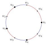
Now assume is odd. Write where is the number of alternating cycles with blues edges (bluish cycles) and is the number of alternating cycles with red edges (reddish cycles).
We start with . Let be a possible bluish cycle of length . It has a single vertex incident to two (potentially) blue edges. From Remark 6.3 it follows that contains exactly vertices from . Without loss of generality, we can express any bluish -cycle as
where , . Indeed, since all have to be distinct, the only common vertex of two blue edges have to be in . Then, exactly one of the two blue edges adjacent to must have both endpoints from . Now we can similarly claim that the number of possible bluish cycles of length is at most . Moreover, the event now determines the values of random vertices , therefore its probability in is . Overall
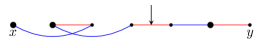
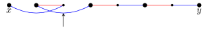
It remains to estimate the expectation of . Let be a possible reddish cycle of length . From Remark 6.3 it follows that the number of -vertices in is either or . Moreover, contains a red -path, and at least one of its endpoints must be from (otherwise there cannot be at least -vertices in ). Let be the red -path, where . It is possible that as well. If then necessarily contains exactly -vertices. Overall we have three different types of possible reddish cycles; we bound the expected number of cycles of each type separately. The three types are demonstrated in Figure 2.
Type 1. There are -vertices and . Cycles of these type behave exactly like even alternating cycles, with one red edge is replaced by a red -path. In this case we relabel and then can be written as
where and . The number of possible cycles of this type is bounded by . Since , the expected number of reddish cycles of type 1 is at most .
Type 2. There are -vertices and . Then there exists a single red edge which has no endpoints in . Let be the sequence of red edges in , starting from and going in the cyclic order. Let be such that is the red edge with no endpoint from . Write . For , write where (so in particular and ) and also let . The blue neighbors of in must be ; without loss of generality, assume the blue edges are and . We get the following cycle:
| (11) |
The conclusion of this analysis is that the number of possible cycles of type 2 is at most the number of choices in the following procedure:
-
1.
Choose an index .
-
2.
Choose a sequence of distinct vertices from and denote them for
-
3.
For choose one of the two red 2-paths starting from it, denote it . If , halt.
-
4.
For every other choose one of the two red edges incident to it, denote it .
-
5.
Choose an additional red edge with no endpoints in . Also choose one of its vertices to be denoted , and denote the second one .
The procedure indeed uniquely defines a possible cycle of type 2: the one described in (11). As explained, every possible cycle of type 2 can be obtained from it. The number of choices in the procedure, which bounds the number of possible cycles of type 2, is at most . Like before, we still have . In conclusion, the expected number of reddish cycles of type 2 is at most
Type 3. There are -vertices and . In this case all red edges have exactly one endpoint from . Moreover, there is a single blue edge which has both endpoints from . The analysis is now similar to the previous type. Again, let be the sequence of red edges in , starting from and going in cyclic order. For write where and also let . There exists such that the blue edge connecting with has both endpoints from (here we let ). We get the following cycle:
| (12) |
So the number of possible cycles of type 3 is at most . As for , it is now bounded by ; the extra factor of comes from the blue edge , which could come from or from . In conclusion, the expected number of reddish cycles of type 3 is at most
In summary, we have proved the following bound for every :
| (13) |
Assume . Then the expected number of alternating cycles of length is
since . Then we are done by Markov’s inequality.
Now assume . Then reddish cycles of type 2 or 3 are impossible, because there is no red path of length with both endpoints in . In that case we can improve (13) and write . Then the expected number of alternating cycles is
Again, we apply Markov’s inequality and complete the proof in the case when is bounded away from .
Finally, assume that and . We apply the bound (13), noting that its proof does not use the fact that is bounded away from . The bound can now be written more neatly as
| (14) |
Let us first prove that w.h.p. there are no alternating cycles of size at least . It immediately follows from the union bound and (14). Note that the power of in this bound is, in particular, due to the inequality . When is linear a much stronger inequality holds true:
where . Note that the function of in the above bound decreases with , and so it is at most . Eventually, we get the following refined bound:
and then Markov’s inequality and the union bound over implies that indeed w.h.p. there are no alternating cycles of length at least . This implies that w.h.p. any union of two alternating cycles has at most vertices from .
Assume that different and are equipotent in . Let as assume that, for a certain , and, at the same time, as well. Due to the description of types of alternating cycles, it may only happen when and are joined in by the path with edges of different color, and the same is true in (an entirely blue might have two consecutive vertices from , and the third vertex should not belong to ). Moreover, both and should be adjacent to at least one blue vertex both in and . Since colours of and are different, . This may only happen when either or belongs to two blue edges in . But then one of these two blue edges joins two vertices from . There can be only constantly many such due to the description of types of alternating cycles.
Then there exists a set of size at least such that, for every , , and . From this it immediately follows that there exists of size at least such that sets and are disjoint and .
Let us now finish the proof. Consider two (not necessarily disjoint) sets and . Assume that the event saying that and are alternating cycles in holds. We may assume that at least vertices of do not belong to . Denote the set of these vertices of that do not belong to any of the cycles by . Almost all (but constantly many) vertices of that belong to the union of the cycles still can play the role of for (unless they do not belong to blue edges with both endpoints from ). We let be the set of such vertices from . Moreover, let , . Recall that .
Note that the set of , , is a uniformly random subset of of size . Let be the number of vertices in . Due to the Hoeffding tail bounds for the hypergeometric distribution (see, e.g. [11, Theorem 2.10]), is at least with probability . Let be the bijection from to that sends to . If, for a certain , , then cycles and cannot be equipotent. Thus, we get that the event that and are equipotent implies that is a bijection between and . Since the probability that coincides with a fixed subset of is , we get the statement of Proposition 6.2 due to the bound (14) and the union bound over the choices of , , , and the directions in both cycles .
∎
In the case , Proposition 6.2 rules out the existence of alternating cycles, which is already sufficient for a proof that is asymmetric w.h.p. (as would be clear from the rest of the proof). In the case , however, we must consider more specific configurations. Thus, for the rest of this subsection, let us assume that where is a positive constant.
Definition 6.5.
For two non-empty sets , the red distance between them is the minimal length of a red path connecting a vertex from to a vertex from .
Definition 6.6.
For a set , , a red segment of of length is a red path with endpoints and internal vertices .
Proposition 6.7.
W.h.p. in , there are no alternating cycles of length at most
-
1.
with an additional alternating path of length between and connecting two (not necessarily distinct) vertices of the cycle;
-
2.
with additional internal edges;
-
3.
with another alternating cycle of length at most at red distance less than ;
-
4.
with a red segment of length between and .
We will need the following claim.
Claim 6.8.
Fix two distinct vertices and let . Let be the number of alternating paths of length which have as the two endpoints. Then
Proof.
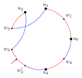
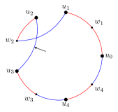
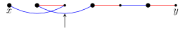
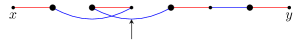
The proof involves case analysis very similar to that of the previous proof. We avoid a repetition of the same details, and instead only briefly describe the different possible types of alternating paths (see also Figure 3).
Again, we distinguish between three cases: even paths, bluish odd paths, and reddish odd paths. Each case can be subdivided into types analogous to the types of reddish cycles from the previous proof.
- Even path
-
consists of red edges and blue edges. Without loss of generality is incident to a blue edge.
- Type E1.
-
and .
- Type E2.
-
and .
- Type E3.
-
and .
- Bluish path
-
consists of red edges and blue edges. At least one endpoint of must be in , due to Remark 6.3. Without loss of generality assume .
- Type B1.
-
and .
- Type B2.
-
and .
- Type B3.
-
and .
- Reddish path
-
consists of red edges and blue edges. In this case we exclude the endpoints of from the count of -vertices, since they are not incident to any blue edge in the path.
- Type R2.
-
.
- Type R3.
-
.
For all types, the expected number of paths is determined (up to a -factor) by combining a factor of for every internal red edge, a factor of for every blue edge, and an additional factor of in types numbered and (coming from the choice of one “special edge”, indicated by an arrow in Figure 3). ∎
Proof of Proposition 6.7.1..
Let be the number of pairs , where is an alternating cycle of length and is an alternating path of length which shares its two endpoints with (internally disjoint from ). A pair can be chosen by first choosing an alternating cycle , then two vertices from , and then an alternating path connecting . From (14) and Claim 6.8, we get
Summing over and , and using the inequality , we deduce . We then apply Markov’s inequality and finish the proof. ∎
Proof of Proposition 6.7.2..
For every , let be the number of pairs where is an alternating cycle of length and is an additional internal red edge. Similarly let be the number of where now is an additional internal blue edge. The idea is that an additional red edge reduces the number of possible choices by a factor of , and an additional blue edge reduces the probability of the existence in by a factor of .
We begin with . First notice that an additional blue edge in is possible only when is odd and is a reddish cycle of type 3 (as defined in the proof of Proposition 6.2). Indeed, in all other cases, the number of blue edges in equals the number of -vertices in , and therefore no additional blue edges may exist. The general form of a reddish cycle of type 3 is described in (12). Using that notation, the additional blue edge must have either or as one of its endpoints. The number of possible choices for is therefore at most (an extra factor of is added due to ). However, the probability that exists in is now . Overall
Now consider . We focus on the case where is even; the odd case is handled similarly and gives an additional factor of .
In any pair the cycle can be labelled as in as in (9) in a way such that has as an endpoint. There are at most ways to choose the other endpoint of . Moreover, determines a red path of length 3 which contains two red edges of , and reduces the number of choices by a factor of . Therefore, a bound on can be obtained by multiplying (10) by , which yields
Recalling that and combining the above,
We apply Markov’s inequality and finish the proof. ∎
Proof of Proposition 6.7.3..
We have already proved that there are no two overlapping alternating cycles w.h.p. Fix and . Let be the number of triplets where are disjoint alternating cycles of lengths respectively, and is a red path connecting them. The idea is that the red path eliminates one degree of freedom in the choice of cycles, therefore reduces the number of choices by a factor of . Let us handle the case when are both even; the odd case is handled similarly, and gives an additional factor of .
Note that together with two red edges from and produce a red path of length , with two vertices from in it. There are ways to choose the path , and this choice determines a red edge of and a red edge of . The number of choices of and of are then reduced by a factor of each. Combining these factors with (10), we obtain the bound
Summing over , and adding a factor of for the odd case, we have
∎
Proof of Proposition 6.7.4..
Fix and . Let count pairs where is an alternating cycle of length and is a red segment of of length . As above, we only consider the case when is even; the odd case is handled similarly, and gves an additional factor of .
Note that the endpoints of are not adjacent by a red edge — otherwise this edge would form with the entire Hamilton cycle. We apply the usual argument: together with the two red edges from produce a red path of length with two vertices from in it. There are ways to choose the path , and this choice determines two red edges of . There are ways to choose their relative position in . The number of choices of is therefore multiplied by a factor of . Combining with (10), we obtain the bound
Summing over , and adding a factor of for the odd case, we have
∎
Finally, we will need the following property.
Proposition 6.9.
W.h.p. in , there exist no two disjoint red paths and of length such that for every .
Proof.
We prove the proposition in the random multigraph . Then, from Proposition 2.10 it is also true in . Moreover, it is sufficient to prove the proposition only for due to monotonicity.
The number of disjoint labelled red paths and is at most . Let us fix such a pair and bound , where
Note that refers to the degree in .
We begin by defining some notation. Let . In , by definition, is distributed uniformly over all subsets of of size . For every , . Let be a random binary vector, whose value precisely determines the intersection of with . We bound by conditioning by the value of .
So, let be a binary vector and consider . Let (the number of -entries in ). Then, given , the subset is distributed uniformly over all subsets of of size . The event is saying that for every . If there exists such that , then of course . Otherwise, we can partition the vertices of into
Then is the event that and .
Now, since for a positive ,
We deduce
This bound is true for every value (uniformly), therefore it also holds for . Now, taking a union bound over the pairs , we have
and that finishes the proof. ∎
6.2 Proof of asymmetry
Let be the group of permutations of . We need to prove that w.h.p., for every , is not an automorphism of . Let be the subgroup of automorphisms of Note that these are exactly the permutations which preserve edge colors.
We begin by proving that w.h.p., no permutation is an automorphism of . Suppose there exists which is an automorphism of . Then there exists a red edge such that is blue. Consider the two red edges incident to ; write them as and . Since is also incident to exactly two red edges, and is red, one of must be blue. Assuming that is blue, and applying the same argument but for applied to , we would get that there exists a red edge such that is blue. Proceeding by induction, we obtain an alternating walk such that its image under is also an alternating walk, with colors switched. Since the graph is finite, at some point the walk meets itself, and we would get an alternating cycle such that is also an alternating cycle, with edge colors switched by . If , we are done: from Proposition 6.2 we know that w.h.p. contains no alternating cycles. So assume for a positive constant . Since labeled and are different, due to Proposition 6.2, we may assume that has length at most .
Let be a vertex in , incident to a red edge and a blue edge in , such that . It is obvious that such a vertex exists when is even. If is odd, then it has a unique vertex adjacent to two edges of the same color. If all other vertices are fixed, then there exists an edge in that maps to itself, and so its image has the same color — a contradiction.
Let be the red edge incident to in . Let be the second red edge incident to . From Proposition 6.7, we may assume that , is red, and all four vertices must be distinct. We can now continue inductively, constructing two disjoint red paths and . Since Proposition 6.7 forbids any red distances or red segments of length at most , in particular we can proceed until the red paths are of length . We get two directed disjoint red paths of length at least with the same sequence of degrees, so Proposition 6.9 applies. We see that the assumption that is -symmetric leads to the existence of one of the rare configurations from the previous subsection in , which happens with probability .
Finally, it remains to show that w.h.p., no permutation is an automorphism of . Recall that these are the permutations which preserve edge colors. This time we separately consider the cases and .
Start with . We show that for a given , the probability that it is an automorphism of is . Then, it would only remain to take a union bound over possible .
We construct a set of vertices (depending only on ) with and and . The construction is done with the following algorithm.
-
1.
Start with .
-
2.
Choose a vertex such that and . Update . Repeat this step times.
-
3.
Choose a vertex such that and . Update . Repeat this step times.
Since is either a rotation or a reflection of the Hamiltonian cycle , it has at most fixed points. Therefore, at the -th step there are at most forbidden vertices. This shows that indeed we can repeat the second step times, and then repeat the third step times. By construction , and . Also let such that and .
Let denote the set of blue edges with an endpoint in and the other endpoint in . If is an automorphism of then the event holds. So it remains to show that, for every possible value of ,
uniformly over .
Consider the vertices . Given , each can still be any vertex from (since ). However, the event restricts to at most possible values from (since there are at most two blue edges between and ). Recall that and that , so given , the event restricts the number of values of each by a factor of . We therefore get the following coarse bound:
In the case we use a different argument. Fix . If is an automorphism of , one of the following events must hold:
-
1.
, the event that for every blue edge .
-
2.
, the event that there exist two blue edges such that .
The first event fully determines the values for every (necessarily , except when is a reflection and there are two fixed points , in which case and ). Therefore .
The second event implies the following event (which is not dependent on ). For every let measure the red distance between and . Let be the event that there exist two distinct vertices such that . It is easy to see that Overall, by the union bound, the probability that is -symmetric in this case is since and . That finishes the proof of Theorem 2.15 for the case .
7 Final remarks
In this paper, we study distinguishability of sparse random graphs by FO sentences. We proved a general upper bound on the minimum quantifier depth of a sentence that distinguishes between independent samples of that answers the question from [4], developed a new tool — random balanced graph — and studied its properties. We observed a new phenomenon: the FO distinguishability between independent samples of depends on how well can be approximated by rational numbers. In particular, from Theorem 1.4 it follows that the lower bound w.h.p. holds true for almost all — in particular, for all algebraic irrational .
We believe that the general upper bound on in Theorem 1.2 can be improved. A possible way to do it is to consider existential sentences that describe existence of a tuple of graphs with a common set of roots defined in such a way that, as soon as, intersections between these graphs become large, the density of their union becomes non-typical. We suspect that a further increase of the width of syntax trees of existential sentences by branching would improve the bound up to , but we do not see a promising way to reach the lower bound in Theorem 1.4.
A more general and involved problem that is very interesting to address is to get a tight dependency between typical values of and an accuracy of approximations of by rational numbers.
References
- [1] László Babai, Paul Erdős, and Stanley M. Selkow. Random graph isomorphism. SIAM J. Comput., 9:628–635, 1980.
- [2] László Babai and Ludik Kučera. Canonical labeling of graphs in linear average time. In 20th IEEE Symp. Found. Computer Sci., pages 39–46, 1979.
- [3] Alan Baker. Transcendental Number Theory. Cambridge University Press, 1975.
- [4] Itai Benjamini and Maksim Zhukovskii. A very sharp threshold for first order logic distinguishability of random graphs. arXiv:2207.11593, 2022.
- [5] Béla Bollobás. The asymptotic number of unlabelled regular graphs. Journal of the London Mathematical Society, 2-26:201–206, 1982.
- [6] Andrzej Ehrenfeucht. An application of games to the completeness problem for formalized theories. Fundamenta Mathematicae, 49(2):129–141, 1961.
- [7] Ronald Fagin. Probabilities on finite models. The Journal of Symbolic Logic, 41(1):50–58, 1976.
- [8] Yury V. Glebskii, Dmitry I. Kogan, M.I. Liogon’kii, and Vladimir A. Talanov. Range and degree of realizability of formulas in the restricted predicate calculus. Cybernetics, 5(2):142–154, 1969.
- [9] Ilay Hoshen and Wojciech Samotij. Simonovits’s theorem in random graphs. arXiv:2308.13455, 2023.
- [10] N. Immerman and E. Lander. The tenacity of zero-one laws. Complexity Theory Retrospective, pages 59–81, 1990.
- [11] Svante Janson, Tomasz Łuczak, and Andrzej Ruciński. Random Graphs. John Wiley & Sons, 2000.
- [12] Aleksandr Khinchin. Einige sätze über kettenbrüche, mit anwendungen auf die theorie der diophantischen approximationen. Mathematische Annalen, 92:115–125, 1924.
- [13] Jeong H. Kim, Oleg Pikhurko, Joel Spencer, and Oleg Verbitsky. How complex are random graphs in first order logic? Random structures & algorithms, 26(1-2):119–145, 2005.
- [14] Jeong Han Kim and Van H. Vu. Concentration of multivariate polynomials and its applications. Combinatorica, 20:417–434, 2000.
- [15] Libkin Leonid. Elements of Finite Model Theory. Texts in Theoretical Computer Science. An EATCS Series. Springer, 2004.
- [16] Brendan D. McKay. Subgraphs of dense random graphs with specified degrees. Combinatorics, Probability and Computing, 20(3):413–433, 2011.
- [17] Oleg Pikhurko, Helmut Veith, and Oleg Verbitsky. The first order definability of graphs: Upper bounds for quantifier depth. Discrete Applied Mathematics, 154(17):2511–2529, 2006.
- [18] Klaus Friedrich Roth. Rational approximations to algebraic numbers. Mathematika, 168(2):1–20, 1955.
- [19] Andrzej Ruciński. Matching and covering the vertices of a random graph by copies of a given graph. Discrete Mathematics, 105:185–197, 1992.
- [20] Andrzej Ruciński and Andrew Vince. Strongly balanced graphs and random graphs. Journal of Graph Theory, 10:251–264, 1986.
- [21] Saharon Shelah and Joel Spencer. Zero-one laws for sparse random graphs. Journal of the American Mathematical Society, 1:97–115, 1988.
- [22] Joel Spencer. The Strange Logic of Random Graphs. Springer, 2001.
- [23] Joel Spencer and Katherine St. John. The tenacity of zero-one laws. Electronic J. Combin., 8(2):14 pp, 2001.
Appendix A Asymmetry: dense case
In this section we prove Theorem 2.16. From now on, suppose that is a sequence of random graphs with the following three properties:
- (P1)
-
.
- (P2)
-
There exists a constant such that for every .
- (P3)
-
There exists a constant such that for every and every .
We need to show that is asymmetric w.h.p.
A.1 Orbits Analysis
Let denote the group of permutations on . For every let denote the probability that is an automorphism of . Then it suffices to show that
| (15) |
To bound for a given permutation , we shall analyize the orbits of edges under the action of .
Definition A.1.
Let . We define a group action of on as follows: for every and ,
Given a permutation and a pair , we define as the orbit of under the action of the subgroup generated by . That is, the -orbit .
Note that for every , the quotient set is
defines a partition of .
The relation between asymmetry of a graph and orbits is given in the following simple claim.
Claim A.2.
as an automorphism of a graph does not split -orbits (that is, for every -orbit , either or ).
The -orbits in the set of edges are closely related to the -orbits in the vertex set , which are simply sets of vertices of cycles in the cycle decomposition of . The following proposition is straightforward.
Proposition A.3.
Let , and where are cycles from the cycle decomposition of . Denote and .
-
•
If then .
-
•
Now suppose and let . Then , unless is even and are opposite in the cycle; in that case .
Proposition A.3 motivates us to classify vertices according to their cycle length in . As it turns out, to properly bound for we must consider -cycles and -cycles separately from the longer cycles.
From now on let us fix a permutation ; all the following definitions are with respect to the action of .
Definition A.4.
We define a partition as follows. are the sets of vertices in -cycles (fixed points), -cycles and -cycles of , respectively. is the set of remaining vertices: vertices in -cycles for . We also write , for and .
Note that is equivalent to .
Definition A.5.
We classify pairs as follows. Suppose where and for some .
-
•
If are not opposite vertices in an even cycle, we say that is a pair of type (and also of type ).
-
•
Now suppose that are opposite vertices in an even cycle of length . Note that then . In this case we say that is a pair of type (and also of type ).
A pair of type is also called an -pair.
Remark A.6.
We make several remarks about the last definition.
-
•
The types and are identical.
-
•
Two pairs in from the same -orbit have the same type. An orbit of an -pair is called an -orbit.
-
•
There are 12 distinct possible types, arranged in the table below.
Definition A.7.
Following the last definitions and remarks, we introduce some additional notations.
-
•
For every type let be the set of -pairs. Also denote .
-
•
For every type , let denote the minimum possible size of an -orbit. The values of for all distinct possible types are arranged in the table below.
A.2 Lists of parameters
We shall bound by taking into account the number of edges of each type in ; we call these numbers the parameters of the graph. Actually, our definition excludes the trivial type from the list of parameters, since it will not contribute anything to the bound. The following definitions are still with respect to a given .
Definition A.8.
Let be the set of all non-trivial distinct types:
Definition A.9.
Let be a graph. Its list of parameters is the -tuple where for every . That is, is the number of edges of type in .
For convenience, lists of parameters are denoted . We also let for every . At this point we slightly deviate from Bollobás’s original definitions, in order to adjust to the non-regular case.
Proposition A.10.
Let be a graph with the list of parameters . For every let be the average degree of vertices from in . Then the following equations hold:
| (16) |
Proof.
The three equations come from counting the sum of degrees of for . From the definition of this sum is . For the right hand side, note that it indeed counts all the edges incident to , with edges with both endpoints in counted twice. The counting is done by considering the different possible types of the edges. ∎
A.3 Bounding
We are now ready for the main part of the proof: bounding , the probability that is an automorphism of . We shall prove a bound which implies Equation (15), and that will finish the proof.
Let be the list of parameters of the random graph .
Definition A.11.
A list is called -valid if
By definition, where the sum is over all -valid lists. To bound , we first bound for a given -valid list .
We fix a -valid list . Then is the probability that, for every , contains exactly edges of type , and also does not split -orbits by Claim A.2.
-
•
Let denote the number of sets of size which can be written as unions of -orbits.
-
•
Let be the number of edges of non-trivial types. Equivalently, is the number of edges incident to .
Proposition A.12.
Following the above definitions, we have
where is the constant from property (P3).
Proof.
There are ways to choose, for every , a set of size which is a union of -orbits. Given such a choice of sets , let . From (P3) we have
The union bound completes the proof. ∎
The following simple combinatorial lemma allows us to bound the terms .
Lemma A.13.
Let be a finite collection of mutually disjoint finite sets, which contains exactly sets of size for every . Suppose there exists a positive integer such that for every . Let denote the number of sets of size which are unions of some of the sets from . Then where is the total size of all sets from .
The proof is fairly straightforward and is given in [5, Equation (5)].
To effectively bound the terms with Lemma A.13, in a way which applies generally for all lists , we must separate “large” from “small” , which motivates the use of below.
Proposition A.14.
For every let and
Then for some positive constant .
Proof.
For every , Lemma A.13 applies where is the set of -orbits, , and . Therefore
When , we are satisfied with the very coarse bound
When , we apply the bound
where . The bound on itself depends on the type . We have three cases:
-
•
. In this case and .
-
•
and . In this case and .
-
•
and . In this case and .
Overall,
∎
Corollary A.15.
For large enough .
Proof.
Due to Proposition A.14, we get
In addition,
for large enough . Inequality follows from Property (P2) of the model (and our assumption that is -valid). Indeed, recall that is the number of edges incident to ; in a graph with maximum degree at most , this number is at most . In Equality we simply define . ∎
The next assertion is the main technical part of the proof.
Lemma A.16.
For every -valid list ,
Note that the bound depends only on , and not on .
Proof.
From Corollary A.15, it suffices to prove
Let us denote
Then we need to prove . Equivalently, we need to prove
| (17) |
Let us bound from below. Denote ; then
| (18) |
At this point we invoke Equations (16). Then
In addition,
As for , we have
and similarly
Again, we apply Equations (16) to write
Overall, putting everything back into (18), we have the following lower bound on . We use colors to help keeping track of the terms.
We write simpler lower bounds on the terms in the brackets. In negative summands with we replace it with . In addition, we omit some positive orange and purple summands.
In there are summands involving . In all six cases, the sum of these summands is of the form where . This is because (unless the respective set is empty, but in that case the corresponding -factor equals 0), which follows from Property (P1) of the model (and our assumption that is -valid). Also note that by definition. Therefore, replacing every appearance of with can only decrease the sum. By doing so (and simplifying) we obtain
The right-hand side can be equivalently rewritten as
Since (unless the respective equals 0), all the numerators in all the fractions above are , so replacing them with only decreases the sum. By doing so, and rearranging summands, we obtain
In conclusion, we have proved Inequality (17), and as explained this completes the proof. ∎
Corollary A.17.
Proof.
We have where the sum is over all -valid lists . Due to Lemma A.16, it only remains to explain why there at most -valid lists .
Every -valid list is a list of non-negative integers, and their sum must satisfy (due to Property (P2) of the model). Therefore, the number of -valid lists is bounded by the number of -tuples of integers, each between and , which is . ∎
We are now ready to prove the asymmetry of .
Proof of Theorem 2.16.
As previously explained, it suffices to prove Equation (15). Let be the set of permutations with non-fixed vertices, vertices in -cycles and vertices in -cycles. Then we shall use the following fairly coarse bound
From Corollary A.17 we deduce
where is some positive constant, since provided by . Every belongs to some set with , and for every there at most choices for such that is non-empty. Overall
Thus the proof is completed. ∎
Appendix B Properties of extensions in random graphs
The following properties of safe and rigid extensions will be useful. For their proofs, see [22, Chapter 4].
Proposition B.1.
Let be a rooted graph.
-
1.
If is not safe then it has a rigid subextension.
-
2.
Assume that is rigid, is a subgraph of some larger graph , and . If then is rigid.
Recall that , , and .
Given an -tuple of vertices , we let denote the random variable which counts -extensions of in . By definition,
where is the number of automorphisms of the rooted graph which preserve the root vertices.
Theorem B.2.
W.h.p. in , for every safe with roots and non-roots, and for every -tuple of vertices , we have uniformly. More explicitly, there exists (which is uniform w.r.t. and ) such that w.h.p.
| (19) |
Proof.
To prove the theorem, we shall prove that there exists such that for any with roots and non-roots and any -tuple , (19) holds with probability , where . Then it would only remain to apply the union bound over and . Indeed, the number of possible safe rooted graphs with roots and non-roots is trivially bounded by . The number of -tuples of vertices is . So the probability of having and such that does not satisfy (19) is
So, from now on let us fix a safe rooted graph of type with roots and , and also fix an -tuple of vertices . Denote . We prove concentration of via Kim and Vu’s powerful concentration result (see [14]). Note that for the rest of the proof, denotes the number of edges in the rooted graph (not the Napier’s constant).
Let be the set of all -tuples which are potential -extensions of . Let be the set of all pairs of vertices which do not connect two vertices of . For every , let be the set of all edges required by the -extension . This is a subset of of size . Finally, for every let be the indicator of the event . Then we can write as the value of a multivariate polynomial on as follows:
For a set of edges with , we define
For every let
Also define
Notice that , thus . Kim-Vu’s concentration result asserts that for every ,
| (20) |
To make use of this result we first bound for every set of edges. It is easy to see that ; let us bound . Consider the set of vertices incident to the edges of , excluding the vertices of ; denote it and its size . We can bound by the number of -tuples which contain all the vertices of (in any positions), which is
If the vertices of and the edges of cannot be completed into an -extension of , then actually is empty and trivially. Otherwise, from safeness of we deduce . Overall .
Comparing to yields
Maximizing over all non-empty sets of at most edges, we obtain the bound
where , with the minimum taken over and .
It is at this point that we encounter the main difference from the original argument: since may now grow with , we get that is no longer constant, but approaches in a way that reflects the behavior of rational approximations of . To provide a lower bound on we invoke the assumption that for all but finitely many rationals . Taking any and (with a finite number of possible exceptions) we have
Overall, this proves the lower bound where is a constant (which comes from the finite number of exceptions). For convenience, we rewrite this lower bound in terms of : since , we have (where now might be a different constant).
We now return to Equation (20). Let us first take care of the left hand side. From what we have seen so far,
Since , we have
We can also trivially bound from above by a constant, and for every , we have . Let us take This choice guarantees
In particular for which does not depend on the specific or .
Remark B.3.
For technical reasons, we also need the following straightforward generalization of Theorem B.2. Following the same notation, w.h.p. for every tuple and every set of “forbidden” vertices of size the conclusion of Theorem B.2 holds for the random variable counting only -extensions of which do not use any vertices from . This generalization can be proved as a direct corollary of Theorem B.2, by adding the forbidden vertices to the rooted graph as roots, without any edges. Technically, this generalization requires the replacement of with , but it has negligible effect on computations since is a constant.
B.1 Proof of Bounded Closure Lemma
The proof is similar to the proof of the Finite Closure Theorem from [22]. For convenience, we present the full argument.
We start by fixing . As in the original argument, set
where the minimum is over all and . Again, this is no longer a positive constant; we now have where is a positive constant.
Define and let us show that with probability , the -closure of any -tuple contains at most vertices. Then, taking a union bound over all possible will finish the proof.
Assume that a set of vertices has . This means there exists a sequence where each is a dense rooted graph of type with and also the number of non-roots of satisfies .
The induced subgraph on has vertices and at least edges. Notice that
It is therefore sufficient to prove the following statement. W.h.p., there exists no subgraph of such that and . Fix a graph which satisfies the above conditions. Its expected number of copies is
since and . Let us recall that and . It is sufficient to take the union bound only over those with minimal number of edges; that is, we may assume . Therefore, the probability of existence of a subgraph of as above is at most
This is since .
B.2 Proof of Lemma 5.8
The idea is to use Theorem B.2 to claim that there are many -extensions, and also that the majority of them must be generic.
From Theorem B.2, Remark B.3, and the Bounded Closure Lemma (with replaced by ), w.h.p. the following properties hold true in :
-
1.
For every safe rooted graph with roots and non-roots, and for every -tuple ,
(21) -
2.
For every -tuple , , letting , we have .
-
3.
For every safe rooted graph with roots and non-roots, and for every -tuple of vertices,
where counts -extensions which do not use any vertex from (we call such -extensions good).
Let be the event that the three conditions above hold; then . We now fix a safe rooted graph with roots and non-roots, a non-negative integer and an -tuple of vertices . To complete the proof, it suffices to show that given the event , has a -generic -extension .
Let denote the type of . Since holds, we know that
where is the number of automorphisms of which preserve the roots. We prove that, given that holds, the number of good -extensions of which fail to be -generic is . First, let us bound the number of good -extensions which violate the first part of Definition 5.7, meaning that they contain additional edges except those specified by . Assume that is such an extension; then it forms an -extension of of type with . This extension cannot have any rigid subextensions, because shares no vertices with . From part 1 of Proposition B.1 it is safe. The number of -extensions of is therefore
The last equality follows from the bound . Summing over possibilities for the rooted graph , we obtain a bound of on the number of -extensions of which violate the first part of Definition 5.7.
Now we bound the number of good -extensions which violate the second part of Definition 5.7. Assume that is such an extension, and let be a rigid extension of with at most nonroots and at least one edge between and . Let denote the rooted graph corresponding to this extension, and let denote its type. Without loss of generality, we may assume that is minimal rigid extension of , in the sense that has no non-trivial rigid subextensions. Note that is an -extension of , which is of type , with . We then consider cases.
Case 1. is safe. The number of -extensions of is
is rigid, so . Actually, we have . Therefore
Summing over possibilities for , we obtain a bound of on the number of which violate the second part of Definition 5.7.
Case 2. is not safe. We first show that in this case, is a rigid extension of . Since is not safe, from part 1 of Proposition B.1 it has a rigid subextension . The vertices of which form this -extension of are actually all in ; we denote them by . Indeed, by definition these vertices are contained in (as they form a rigid extension of with at most vertices) but contains no vertices from . From part 2 of Proposition B.1 we deduce that is a rigid extension of . It corresponds to a rigid subextension of , but from minimality it must be itself, so . Therefore is a rigid extension of .
Now, since is a rigid extension of , its vertices are all in . Since has at most vertices and , there are possibilities for .
Fix a possible . Consider as an extension of . It does not have a rigid subextension, since contains no vertex from , and from part 1 of Proposition B.1 it is safe. Let denote the rooted graph corresponding to this extension. Its type is with , because there is at least one edge between and . Its number of roots is at most . Therefore the number of -extensions of is
Summing over possibilities for the rooted graph and possibilities for , we get a bound of on the number of which violate the second part of Definition 5.7. That completes the proof.