Tree-Packing Revisited: Faster Fully Dynamic Min-Cut and Arboricity

A tree-packing is a collection of spanning trees of a graph. It has been a useful tool for computing the minimum cut in static, dynamic, and distributed settings. In particular, [Thorup, Comb. 2007] used them to obtain his dynamic min-cut algorithm with $\tilde{O}(\lambda^{14.5}\sqrt{n})$ worst-case update time. We reexamine this relationship, showing that we need to maintain fewer spanning trees for such a result; we show that we only need to pack $\Theta(\lambda^{3}\log m)$ greedy trees to guarantee a 1-respecting cut or a trivial cut in some contracted graph.

Based on this structural result, we then provide a deterministic algorithm for fully dynamic exact min-cut, that has $\tilde{O}(\lambda^{5.5}\sqrt{n})$ worst-case update time, for min-cut value bounded by $\lambda$. In particular, this also leads to an algorithm for general fully dynamic exact min-cut with $\tilde{O}(m^{1-1/12})$ amortized update time, improving upon $\tilde{O}(m^{1-1/31})$ [Goranci et al., SODA 2023].

We also give the first fully dynamic algorithm that maintains a $(1+\varepsilon)$-approximation of the fractional arboricity – which is strictly harder than the integral arboricity. Our algorithm is deterministic and has $O(\alpha\log^{6}m/\varepsilon^{4})$ amortized update time, for arboricity at most $\alpha$. We extend these results to a Monte Carlo algorithm with $O(\operatorname{\text{{\rm poly}}}(\log m,\varepsilon^{-1}))$ amortized update time against an adaptive adversary. Our algorithms work on multi-graphs as well.

Both result are obtained by exploring the connection between the min-cut/arboricity and (greedy) tree-packing. We investigate tree-packing in a broader sense; including a lower bound for greedy tree-packing, which – to the best of our knowledge – is the first progress on this topic since [Thorup, Comb. 2007].

1 Introduction

A tree-packing is a collection of spanning trees of a graph. Often one is interested in a tree-packing satisfying certain requirements, e.g., greedy, disjoint, which we detail where applicable. In particular, tree-packing first appeared in the seminal works of Nash-Williams [NW61] and Tutte [Tut61]. They studied sufficient and necessary conditions for when a graph can be decomposed into $k$ disjoint spanning subgraphs, i.e., when a graph admits a disjoint tree-packing of size $k$. They provided a sufficient and necessary condition by considering partition values: given a partition $\mathcal{P}$ of the vertex set of a graph $G$, the value of $\mathcal{P}$ is then $\tfrac{|E(G/\mathcal{P})|}{|V(G/\mathcal{P})|-1}$ , where $G/\mathcal{P}$ is the graph obtained by contracting $\mathcal{P}$ in $G$. In particular, they showed that $G$ admits a decomposition into $k$ disjoint spanning trees if and only if the minimum partition value is at least $k$. Not long after, Nash-Williams noted [NW64] that his techniques extends to answer a question with a very similar flavor: what is the smallest number of trees needed to cover all edges of a graph? This number is now known as the arboricity of the graph, and Nash-Williams showed that the arboricity is the ceiling of the fractional arboricity defined as $\alpha:=\max_{S\subseteq V}\frac{|E(S)|}{|S|-1}$.

Tree-packing, however, has not only been studied for its mathematical properties, but also for its algorithmic applications. In a seminal paper, Gabow [Gab95] showed how related techniques can be used to compute both a packing of disjoint trees and the minimum cut value of a graph, i.e., the minimum number of edges whose deletion causes the graph to become disconnected. Such a collection of edges form a minimum cut or min-cut for short. This was far from the end of the story, as Karger [Kar00] used the fact that any large enough greedy tree-packing contains trees that $2$-respect some min-cut, i.e., it contains a spanning tree which crosses some min-cut at most twice. Here a greedy tree-packing is defined as follow: let the weight of an edge be the number of trees an edge belongs to, and require that the spanning trees in the packing form successive minimum spanning trees. To arrive at his near-linear time min-cut algorithm for computing a min-cut, Karger used this fact by showing that one can efficiently compute the size of all cuts that $2$-respects a tree. This observation has subsequently also found use for computing $k$-cuts [Tho08, CQX19].

This ‘semi-duality’ between tree-packing and min-cut has also found applications in other models of computation such as distributed computing [DHNS19, DEMN21] and in dynamic algorithms [TK00, Tho07]. Dynamic algorithms maintain a solution to a problem – for instance the size of a min-cut – as the input graph undergoes deletions and insertions of edges. In this setting, it is not known how to maintain the smallest $2$-respecting cut in a dynamic forest. Instead, Thorup [Tho07] showed that packing $\Omega(\lambda^{7}\log^{3}m)$ greedy trees is sufficient to guarantee that at least one tree $1$-respects a min cut, provided that the size of the min-cut is at most $\lambda$. He then shows that one can dynamically maintain this packing in $\tilde{O}(|\mathcal{T}|^{2}\sqrt{\lambda n})$ update time and that one can maintain the smallest $1$-respecting cut efficiently in a dynamic forest. These things combine to give an exact dynamic algorithm running in $\tilde{O}(\lambda^{14.5}\sqrt{n})$ worst-case update time, whenever the min-cut has size at most $\lambda$.

This dependency on $\lambda$ is persistent. Even the cases $\lambda=1$ and $\lambda=2$ are important and very well-studied in the dynamic setting [Fre85, GI91, WT92, EGIN97, Fre97, HK97, HK99, HLT01, KKM13, NSW17, HRT18, CGLN+20]. Recently Jin, Wu, and Thorup [JST24] gave an algorithm for the case that $\lambda\leq(\log m)^{o(1)}$. For general (polynomial) values of $\lambda$, Thorup [Tho07] remains the state-of-the-art. One immediate way of improving the dependency on $\lambda$ in his update time is to show that packing even fewer trees still guarantees that at least one tree $1$-respects a min-cut. This prompted Thorup to ask if it is possible to show that an even smaller tree-packing always $1$-respects at least one min-cut. In recent work, Goranci et al. [GHNS+23] balanced the approach of Thorup with a different approach based on expander decompositions to get an exact dynamic algorithm for all values of $\lambda$. Again, an improvement in the $\lambda$ dependency immediately yields a faster algorithm. In a similar vein to Thorup, they asked whether this is possible.

In this paper, we answer this question in the affirmative. We show that focusing solely on $1$-respecting cuts might be too limited an approach in the dynamic setting. In particular, we show that in the cases where one might need to pack many trees to ensure that at least one packed tree $1$-respects a min-cut, one can instead consider a corresponding approximate partition. We show that whenever, we cannot guarantee a $1$-respecting min-cut, we can instead guarantee that the approximate partition contains a trivial min-cut. We then make this approach algorithmic by showing how to maintain the trivial min-cuts of this approximate partition. By doing so, we need only pack $\Omega(\lambda^{3}\log m)$ trees, thus resulting in a much smaller final dependency on $\lambda$.

In spite of tree-packing having found so many applications, we are still far from fully understanding them and their limits. In this paper, we show that they are not only useful for dynamically estimating the min-cut, but also for dynamically estimating the fractional arboricity, as we provide the first dynamic algorithm able to $(1+\varepsilon)$-approximate the fractional arboricity efficiently. Finally, we study the limits of tree-packing based approaches by proving some technical results concerning tree-packing. As such, we categorize our results in three sections: dynamic min-cut, dynamic arboricity, and technical results concerning tree-packing.

1.1 Min-Cut

First, we present our results for dynamic min-cut. We obtain the following result. theoremmincutPar There exists a deterministic dynamic algorithm, that given an unweighted, undirected (multi-)graph $G=(V,E)$, maintains the exact min-cut value $\lambda$ if $\lambda\leq\lambda_{\max}$ in $\tilde{O}(\lambda_{\max}^{5.5}\sqrt{n})$ worst-case update time.
It can return the edges of the cut in $O(\lambda\log m)$ time with $\tilde{O}(\lambda_{\max}^{5}\sqrt{m})$ worst-case update time. This improves on the state-of-the-art by Thorup [Tho07], who achieves $\tilde{O}(\lambda_{\max}^{14.5}\sqrt{n})$ worst case-update time. Thorup also uses this result to obtain $(1+\varepsilon)$-approximate min-cut against an oblivious adversary in $\tilde{O}(\sqrt{n})$ time, where our result improves the polylogarithmic factors. An application where our result has more impact is deterministic exact min-cut for unbounded min-cut value $\lambda$.

theoremmincutCombi There exists a deterministic dynamic algorithm, that given a simple, unweighted, undirected graph $G=(V,E)$, maintains the exact min-cut value $\lambda$ with amortized update time

$$\tilde{O}(\min\{m^{1-1/12},m^{11/13}n^{1/13},n^{3/2}\}).$$

It can return the edges of the cut in $O(\lambda\log m)$ time with $\tilde{O}(m^{1-1/12})$ amortized update time. We obtain this result by using the algorithm of Goranci et al. [GHNS+23] for the high $\lambda$ regime. When they combine this with [Tho07], they achieve $\tilde{O}(m^{29/31}n^{1/31})=\tilde{O}(m^{1-1/31})$ amortized update time. We note that Goranci et al. [GHNS+23] also provide a randomized result with $\tilde{O}(n)$ worst-case update time against an adaptive adversary.

Further Related Work.

Jin and Wu [JS21] gave an algorithm for $s-t$ min-cut, for min-cut up to size $(\log m)^{o(1)}$ with $n^{o(1)}$ worst-case update time. Recently, they generalized these techniques to get $n^{o(1)}$ worst-case update time for the global min-cut [JST24] up to size $(\log m)^{o(1)}$. There is a further line of work on smaller values of the min-cut: in particular for graph connectivity (whether $\lambda\geq 1$) [Fre85, HK99, HLT01, KKM13, NSW17, CGLN+20] and 2-edge connectivity (whether $\lambda\geq 2$) [WT92, GI91, EGIN97, Fre97, HK97, HLT01, HRT18].

For planar graphs, Lacki and Sankowski [LS11] provided a deterministic algorithm with $\tilde{O}(n^{5/6})$ worst-case update and query time.

There are faster algorithms for dynamic min-cut, at the cost of an approximation factor: Karger and Thorup [TK00] gave a $(2+\varepsilon)$-approximation in $\tilde{O}(\operatorname{\text{{\rm poly}}}(\log m,\varepsilon^{-1}))$ amortized update time, and Thorup [Tho07] gave a $(1+\varepsilon)$-approximation in $\tilde{O}(\sqrt{n})$ worst-case update time.

In the partially dynamic setting, Thorup [Tho07] gives an algorithm with $\tilde{O}(n^{3/2}+m)$ total time for the purely decremental and incremental settings. Further, there are incremental algorithms with $O(\lambda\log m)$ or $O(\operatorname{\text{{\rm poly}}}\log m)$ amortized update time, by Henzinger [Hen97] and Goranci, Henzinger, and Thorup [GHT18] respectively.

1.2 Arboricity

The fractional arboricity $\alpha$ of a graph is defined as

$$\alpha:=\max_{S\subseteq V}\frac{|E(S)|}{|S|-1}.$$

The arboricity is defined as $\lceil\alpha\rceil$, so strictly easier to compute. Equivalently, we can define the arboricity as the minimum number of trees needed to cover the graph [NW61].

Our Result.

We provide an algorithm to compute the arboricity based on tree-packing. This leads to the first dynamic $(1+\varepsilon)$-approximation of the fractional arboricity. Our algorithm is deterministic, hence also works naturally against an adaptive adversary.

theoremarboricityDetNew There exists a deterministic dynamic algorithm, that given an unweighted, undirected (multi-)graph $G=(V,E)$, maintains a $(1+\varepsilon)$-approximation of the fractional arboricity $\alpha$ when $\alpha\leq\alpha_{\max}$ in $O(\alpha_{\max}\log^{6}m/\varepsilon^{4})$ amortized update time or a Las Vegas algorithm with $O(\alpha_{\max}^{2}m^{o(1)}/\varepsilon^{4})$ worst-case update time. This improves the approximation factor in the state-of-the-art: Chekuri et al. [CCHH+24] give a $(2+\varepsilon)$-approximation of the fractional arboricity. It has $O(\log\alpha_{\max}\log^{2}m/\varepsilon^{4})$ amortized update time or $O(\log\alpha_{\max}\log^{3}m/\varepsilon^{6})$ worst-case update time. In fact, for simple graphs, the value of the densest subgraph is a $(1+\varepsilon)$-approximation for large values of $\alpha$. Combining this with our result for smaller values of $\alpha$, we obtain the following result.

theoremarboricitySimple There exists a deterministic dynamic algorithm, that given a simple, unweighted, undirected graph $G=(V,E)$, maintains a $(1+\varepsilon)$-approximation of the fractional arboricity $\alpha$ in $O(\log^{6}m/\varepsilon^{5})$ amortized update time or a Las Vegas algorithm with $O(m^{o(1)}/\varepsilon^{6})$ worst-case update time.

For multi-graphs, the value of the densest subgraph remains a $2$-approximation of the fractional arboricity, even when $\alpha$ becomes large. To obtain an efficient algorithm for $(1+\varepsilon)$-approximation, we use a sampling technique to reduce the case of large $\alpha$ to the case of small $\alpha$. Although this is rather straight-forward against an oblivious adversary, we need to construct a more sophisticated scheme to deal with an adaptive adversary.

theoremarboricity There exists a dynamic algorithm, that given an unweighted, undirected (multi-)graph $G=(V,E)$, maintains a $(1+\varepsilon)$-approximation of the fractional arboricity $\alpha$ against an adaptive adversary in $O(\log^{11}m/\varepsilon^{15})$ amortized update time or $O(m^{o(1)}/\varepsilon^{19})$ worst-case update time.

Against an oblivious adversary we obtain the improved amortized update time of $O(\log^{7}m/\varepsilon^{6})$, or worst-case update time $O(m^{o(1)}/\varepsilon^{8})$, see Section 3.4.

We remark that the update time of many dynamic algorithms is parameterized by the (fractional) arboricity [BF99, BS15, BS16, CCHH+24, KKPS14, NS16, PS16]. This shows that the fractional arboricity is an important graph parameter. These algorithms are faster when $\alpha$ is small, and this is exactly the regime where dynamic approximations of $\alpha$ are lacking. We hope that our results contribute to a better understanding of this.

Further Related Work.

Computing the (fractional) arboricity of a graph is a relatively hard problem; we do not know a static linear-time algorithm for the exact version. Gabow showed how to compute the arboricity in $\tilde{O}(m^{3/2})$ time [Gab95, Gab98]. For the approximate version, much faster algorithms are known. In particular, Eppstein gave a $2$-approximation in $O(m+n)$ time [Epp94].

Plotkin, Shmoys, and Tardos gave a FPTAS for solving fractional packing and fractional covering problems, and their algorithm applied to fractional arboricity takes $\tilde{O}(m\alpha/\varepsilon^{2})$ time [PST95] and provides a $(1+\varepsilon)$-approximation, where $\alpha$ denotes the value of the fractional arboricity. Toko, Worou, and Galtier gave a $(1+\varepsilon)$-approximation for the fractional arboricity in $O(m\log^{3}m/\varepsilon^{2})$ time [TWG16]. Blumenstock and Fischer [BF20] gave a $(1+\varepsilon)$-approximation of the arboricity in $O(m\log m\log\alpha/\varepsilon)$ time. More recently, Quanrud [Qua24] gave a $(1+\varepsilon)$-approximation of the arboricity w.h.p. in $O(m\log m\alpha(n)+n\log m(\log m+(\log\log m+\log(1/\varepsilon))\alpha(n))/\varepsilon^{3})$ time, where $\alpha(n)$ is the inverse Ackermann.

The exact fractional arboricity can be computed in $\tilde{O}(mn)$ time [Gab98].

For dynamic arboricity, there is a deterministic exact algorithm with worst-case update time $\tilde{O}(m)$ [BRS20]. The work of Brodal and Fagerberg [BF99] implies a $4$-approximation of the arboricity in $O(\operatorname{\text{{\rm poly}}}\log m)$ amortized update time against an oblivious adversary.

Both for better approximations, and for the fractional arboricity, we turn to the closely related densest subgraph problem, where we want to determine the density $\rho$:

$$\rho:=\max_{S\subseteq V}\frac{|E(S)|}{|S|}.$$

There have been multiple dynamic approximate densest subgraph algorithms over the last years [ELS15, BHNT15, SW20]. The state-of-the-art [CCHH+24] gives a $(1+\varepsilon)$-approximation, which in turn imply $(2+\varepsilon)$-approximate fractional arboricity algorithms (for simple graphs). It has $O(\log^{2}m\log\rho/\varepsilon^{4})$ amortized update time or $O(\log^{3}m\log\rho/\varepsilon^{6})$ worst-case update time.

The algorithms via densest subgraph, but also [BF99], use out-orientations to compute the approximate fractional arboricity. Although this works well for crude approximations, it seems to not lead to high precision approximations.

1.3 Tree-Packing

Definitions.

Let $V=(G,E)$ an unweighted undirected graph. A tree-packing $\mathcal{T}$ of $G$ is a family of spanning trees, where edges can appear in multiple trees. The load of an edge $e$, denoted by $L^{\mathcal{T}}(e)$, is defined by the number of trees that contain $e$. The relative load is defined as $\ell^{\mathcal{T}}(e)=L^{\mathcal{T}}(e)/|\mathcal{T}|$. Whenever the tree-packing is clear from the context, we omit the superscript $\cdot^{\mathcal{T}}$. The packing value of a tree-packing $\mathcal{T}$ is

$$\rm{pack\_val}(\mathcal{T}):=\frac{1}{\max_{e\in E}\ell^{\mathcal{T}}(e)}.$$

Dual to tree-packing we have a concept for partitions. For a partition $\mathcal{P}$, we define the partition value as

$$\rm{part\_val}(\mathcal{P}):=\frac{|E(G/\mathcal{P})|}{|\mathcal{P}|-1}.$$

We now have that (see e.g. [NW61, Tut61])

$$\Phi_{G}:=\max_{\mathcal{T}}\rm{pack\_val}(\mathcal{T})=\min_{\mathcal{P}}\rm{part\_val}(\mathcal{P}).$$

We omit the subscript and simply write $\Phi$ when the graph is clear from the context.

Next, we introduce ideal relative loads, following Thorup [Tho07]. These loads, denoted by $\ell^{*}(e)$, are defined recursively.

1. Let $\mathcal{P}^{*}$ be a packing with $\rm{pack\_val}(\mathcal{P}^{*})=\Phi$.

2. For all $e\in E(G/\mathcal{P})$, set $\ell^{*}(e):=1/\Phi$.

3. For each $S\in\mathcal{P}^{*}$, recurse on the subgraph $G[S]$.

Greedy Tree-Packing.

Thorup [Tho07] showed that a greedy tree-packing approximates the ideal packing well. In particular, a greedy tree-packing $\mathcal{T}$ with $|\mathcal{T}|\geq 6\lambda\log m/\varepsilon^{2}$ trees satisfies

$$|\ell^{\mathcal{T}}(e)-\ell^{*}(e)|\leq\varepsilon/\lambda,$$ (1)

for all $e\in E$.

Now he continues to show, that if we pack $\Omega(\lambda^{7}\log m)$ greedy trees, we pack at least one tree that crosses some min-cut only once. This argument heavily relies on Equation 1 with $\varepsilon$ set to $\lambda^{3}$.

Tree-Packing and Min-Cut.

Instead of directly improving upon the bounds above, i.e., showing that one can pack fewer trees, we investigate the relationship between tree-packing and min-cut more closely.

theoremthmCutExistence Let $G$ be an unweighted, undirected (multi-) graph, and let $\mathcal{T}$ be a tree-packing on $G$. Suppose $|\mathcal{T}|=\Omega(\lambda^{3}\log m)$, then at least one of the following holds

1. Some $T\in\mathcal{T}$ $1$-respects a min-cut of $G$; or

2. Some trivial cut in $G/\{e\in E:\ell^{\mathcal{T}}(e)<\tfrac{2}{\lambda}-\tfrac{3}{8\lambda^{2}}\}$ corresponds to a min-cut of $G$.

This result is the main technical ingredient for Section 1.1, which also contains novel dynamic routines for maintaining both parts.

Number of Greedy Trees.

First of all, we can show that packing many greedy trees is actually necessary to satisfy Equation 1 (up to a $\log m$ factor).

theoremTPlowerbound Let $G$ be an unweighted, undirected (multi-) graph. In general, a greedy tree-packing $\mathcal{T}$ needs $|\mathcal{T}|=\Omega(\lambda/\varepsilon^{{3}/{2}})$ trees to satisfy

$$|\ell^{\mathcal{T}}(e)-\ell^{*}(e)|\leq\varepsilon/\lambda,$$

for all $e\in E$, whenever $\varepsilon^{-1}=O(n^{1/3})$.

A Smaller Tree-Packing.

For a general tree-packing, clearly $\lambda/\varepsilon$ is a lower bound for the number of trees to satisfy Equation 1. We show that there always exists a tree-packing satisfying this.

theoremTPexistence Let $G$ be an unweighted, undirected (multi-)graph. There exists a tree-packing $\mathcal{T}$ with $|\mathcal{T}|=\Theta(\lambda/\varepsilon)$ trees that satisfies

$$|\ell^{\mathcal{T}}(e)-\ell^{*}(e)|\leq\varepsilon/\lambda,$$

for all $e\in E$. Although a greedy tree-packing is easy to compute and maintain, this might indicate that investigating other tree-packings might be worthwhile.

Further Related Work.

Tree-packing can be formulated as a (packing) LP. One way of solving LPs is via the Multiplicative Weights Update (MWU) Method, see e.g., [AHK12]. In particular, this method needs at most $O(\rho\log m/\varepsilon^{2})$ iterations for a packing/covering LP with width $\rho$ [PST95]. For tree-packing, we have width $\rho=\Theta(\lambda)$.

The MWU method and greedy tree-packing are strongly related. In particular, Harb, Quanrud, and Chekuri [HQC22] note that if one uses (a particular version of) the MWU method then the resulting algorithm would also be greedy tree-packing. Chekuri, Quanrad, and Xu [CQX20] conjecture that greedy tree-packing is in fact equivalent to approximating the LP via the standard MWU method.

General packing LPs have an iteration count lower bound of $\Omega(\rho\log m/\varepsilon^{2})$ iterations [KY15]. It is unclear whether this also holds for the special case of tree-packing. We think it is likely that our lower bound, Section 1.3, can be extended with a factor $\log m$. However, we think that the $\varepsilon$ dependency might be optimal. In other words, we conjecture that the MWU method for tree-packing requires $\Theta(\lambda\log m/\varepsilon^{3/2})$ iterations.

We note that in both greedy tree-packing and in the MWU method, there is still freedom in the update step: in greedy tree-packing there are often multiple minimum spanning trees (e.g., the first tree can be any spanning tree) and in the MWU method we can select multiple constraints. So, although we do not expect every greedy tree-packing to perform better, we might still be able to show that a specific greedy tree-packing beats the general lower bound. For example, selecting a minimum spanning tree at random.

Tree-packing is also used for minimum $k$-cut [NR01, CQX20]. It is an interesting open question whether our techniques extend to this setting.

1.4 Technical Overview

Dynamic Graph Algorithms.

Before we give an overview of our techniques, we recall the model we are working in. The goal is to maintain a data structure for a changing graph, that maintains the solution to some problem, e.g., the value of the min-cut or the arboricity. The input graph undergoes a series of updates, which are either edge insertions or edge deletions. If the sequence of updates is fixed from the start, we say we have an oblivious adversary. If the sequence of updates can be based upon the algorithm or the state of the data structure, we say we have an adaptive adversary. We say the algorithm has amortized update time equal to $t$, if it spends $O(\sigma t)$ time for a series of $\sigma$ updates. We say the algorithm has worst-case update time equal to  $t$ if it spends at most $t$ time after every update.

In some cases, the data structure does not store the solution to the problem explicitly, but it can be retrieved by a query, e.g., in case of the edges of a min-cut. In this case we state the required time to answer such a query.

1.4.1 Min-Cut

To obtain our dynamic min-cut result, Section 1.1, we have three technical contributions. The first is showing Section 1.3. Our algorithm then consists of maintaining such a tree-packing, its 1-respecting cuts, and the corresponding trivial cuts. Our second contribution is showing how to maintain such trivial cuts, and the third is a new technique to decrease the recourse of tree-packing.

Min-Cut and Tree-Packing.

First, let us sketch the proof of Section 1.3. The main observation that allows one to show that some tree $1$-respects a min-cut is that if some min-cut $C$ has

$$\sum_{e\in C}\ell^{\mathcal{T}}(e)<2,$$

then it must be $1$-respected by some tree. Indeed, then the average number of times a tree in $\mathcal{T}$ crosses $C$ is

$$\frac{1}{|\mathcal{T}|}\sum_{e\in C}L^{\mathcal{T}}(e)=\sum_{e\in C}\ell^{\mathcal{T}}(e)<2,$$

so some tree must $1$-respect $C$. Hence, if $\sum_{e\in C}\ell^{*}(e)$ is small enough, i.e., far enough below $2$, then the tree-packing does not need not be very large to also concentrate the sum $\sum_{e\in C}\ell^{\mathcal{T}}(e)$ below $2$.

Hence, we can restrict ourselves to the case where every min-cut $C$ has $\sum_{e\in C}\ell^{*}(e)\approx 2$. In this case, one can show that in fact every edge $e$ participating in a min-cut has $\ell^{*}(e)\geq\bar{a}\approx\tfrac{2}{\lambda}$ for some appropriately chosen $\bar{a}$. This in turn means that for a different value $\hat{a}$ only slightly smaller than $\bar{a}$, the graph $G/\{e\in E:\ell^{*}(e)<\hat{a}\}$ must contain trivial min-cuts. To show this we assume this is not the case for contradiction, and then count the edges of the graph in two different ways: once using the $\ell^{*}$ values and once by summing the degrees. The first way of counting implies that $G/\{e\in E:\ell^{*}(e)<\hat{a}\}$ contains roughly $\hat{a}^{-1}|V(G/\{e\in E:\ell^{*}(e)<\hat{a}\})|\approx\tfrac{\lambda}{2}|V(G/\{e\in E:\ell^{*}(e)<\hat{a}\})|$ edges, and the second way of counting shows via the Hand-Shaking Lemma that $G/\{e\in E:\ell^{*}(e)<\hat{a}\}$ contains at least $\tfrac{\lambda+1}{2}|V(G/\{e\in E:\ell^{*}(e)<\hat{a}\})|$ – a contradiction.

The rest of the proof then boils down to showing that for an arbitrary trivial min-cut $X$ of $G/\{e\in E:\ell^{*}(e)<\hat{a}\}$, $\Phi_{G[X]}$ is sufficiently large. Indeed, this implies that we do not need to pack too many trees in order to concentrate $\ell^{\mathcal{T}}$ values of the edges in a min-cut far above the $\ell^{\mathcal{T}}$ values of edges in $G[X]$. In particular, one can ensure that all edges $e$ in a min-cut have $\ell^{\mathcal{T}}(e)>\hat{a}$ and all edges in $G[X]$ has $\ell^{\mathcal{T}}(e)<\hat{a}$. This then implies that $X$ is a trivial min-cut of $G/\{e\in E:\ell^{\mathcal{T}}(e)<\hat{a}\}$.

To show this, we lower bound the value of $\Phi_{G[X]}$ via the objective value of an optimization problem, which encodes the size of every trivial cut in the partition $\mathcal{P}$ realizing $\Phi_{G[X]}$. The key property needed is that no min-cut edges are in $E(G[X])$ and so very few trivial cuts of $G[X]/\mathcal{P}$ have size smaller than $\lambda+1$. This allows us to bound the objective value of the optimization problem significantly above $\tfrac{\lambda}{2}$, which in turn implies that all $\ell^{*}$ values of edges in $G[X]$ are significantly below $\tfrac{2}{\lambda}$, thus yielding the required property. For more details, see Section 2.1.

Maintaining Trivial Cuts.

Second, we describe how we maintain the trivial cuts efficiently. The key challenge in maintaining the size of the trivial cuts, is that we do not know how to maintain an explicit representation of $G/\{e\in E:\ell^{*}(e)<\hat{a}\}$. The difficult part is that dynamically maintaining contractions and un-contractions explicitly can be very time consuming, as we might need to look at many edges in order to assign them the correct endpoints after the operation is performed. To circumvent this issue, we maintain a weaker, implicit representation of $G/\{e\in E:\ell^{*}(e)<\hat{a}\}$. Instead of maintaining the graph explicitly, we only maintain the vertices of $G/\{e\in E:\ell^{\mathcal{T}}(e)<\hat{a}\}$ as well as their degrees. This weaker representation turns out to be much easier to maintain.

We maintain a dynamic connectivity data structure on the graph induced by all edges $e$ with $\ell^{\mathcal{T}}(e)<\hat{a}$. The connected components of this graph correspond exactly to the vertices of $G/\{e\in E:\ell^{\mathcal{T}}(e)<\hat{a}\}$. In order to calculate the degree of these vertices, we maintain the number of edges $e$ with $\ell^{\mathcal{T}}(e)\geq\hat{a}$ incident to each vertex $v\in V(G)$. Since the connectivity data structure supplies us with a connectivity witness in the form of a spanning forest, we can maintain a spanning tree of each connected component as a top tree [AHLT05]. By weighting each vertex $v\in V(G)$ by the number of incident edges $e$ with $\ell^{\mathcal{T}}(e)\geq\hat{a}$, we can use the top trees to dynamically maintain the sum of vertex weights of each tree. Since loops are counted twice, the sum of vertex weights in a spanning tree correspond exactly to the degree of the corresponding vertex in $G/\{e\in E:\ell^{\mathcal{T}}(e)<\hat{a}\}$. By using a min-heap, we can then maintain the minimum degree of $G/\{e\in E:\ell^{\mathcal{T}}(e)<\hat{a}\}$, which can only over-estimate the size of the corresponding trivial cut. To report the min-cut, we can then retrieve the cut by searching each vertex with weight strictly greater than $0$ in only $\log m$ time, and then report each edge with $\ell^{\mathcal{T}}(e)\geq\hat{a}$ incident to the vertex in $\log m$ time per edge. For more details, see LABEL:sc:trival_cuts.

Recourse in Tree-Packing.

Third, we turn to the tree-packing. We note that the most expensive step in our algorithm is to maintain $1$-respecting cuts on $|\mathcal{T}|=\Theta(\lambda_{\max}^{3}\log m)$ minimum spanning trees. Every time such a spanning tree changes, we need to update its $1$-respecting cuts in $\tilde{O}(\sqrt{n})$ time. Therefore, it is important to bound the recourse in these spanning trees: the number of changes to the tree-packing due to an edge update. Naively, we have $O(|\mathcal{T}|^{2})=O(\lambda_{\max}^{6}\log^{2}m)$ recourse (see e.g., [TK00]), to see this consider an edge deletion. This edge is contained in at most $|\mathcal{T}|$ trees. In each of these trees it needs to be replaced, which leads to a weight increase for the replacement edge. This change needs to be propagated in all following trees, so can lead to a series of $|\mathcal{T}|$ changes. We show that we can get away with a recourse of $O(\lambda_{\max}^{5}\log^{2}m)$. See LABEL:lm:TP_recourse_impr for a formal statement. This improvement is independent of the improvement from Section 1.3 in the number of trees we need to pack, and might have applications in other instances where a greedy tree-packing is used.

The first observation is that if the graph has min-cut $\lambda$, then an edge will be in roughly $|\mathcal{T}|/\lambda$ trees, not in all $|\mathcal{T}|$. If $\lambda=\lambda_{\max}$ throughout the update sequence, then this gives the result. However, $\lambda$ can become arbitrary small. To mitigate this fact, we keep $\log\lambda_{\max}$ copies of the tree-packing, $\mathcal{T}_{1},\mathcal{T}_{2},\dots$, where $\mathcal{T}_{i}$ corresponds to the case where the min-cut value is in $[2^{i},2^{i+1})$. If $\lambda\geq 2^{i}$, then we have $\mathcal{T}_{i}$ as a normal tree-packing on $G=(V,E)$. However, if $\lambda<2^{i}$, then $\mathcal{T}_{i}$ is a tree-packing on $(V,E\cup E_{\rm{virtual}})$, where $E_{\rm{virtual}}$ is some set of virtual edges ensuring that the min-cut stays large. These edges get added as $\lambda$ shrinks and deleted as $\lambda$ grows.

When using this global view of the connectivity, we obtain an algorithm with $O(\lambda_{\max}^{5}\log^{2}m)$ amortized recourse. However, by inspecting the $\ell^{\mathcal{T}}$ values, we have a much more refined view of the connectivity. With a careful analysis, this means we can obtain the same bound on the worst-case recourse. This comes down to deleting a virtual edge when it is no longer needed, and not waiting until the global min-cut has increased. We refer to LABEL:sc:TP_recourse for the details.

1.4.2 Arboricity

We revisit the relationship between ideal tree-packing and the partition values. We recall that [NW61, Tut61]

$$\Phi_{G}:=\max_{\mathcal{T}}\rm{pack\_val}(\mathcal{T})=\min_{\mathcal{P}}\rm{part\_val}(\mathcal{P}),$$

which Thorup [Tho07] used to recursively define the ideal relative loads $\ell^{*}$. By a close inspection of these definitions, we can show that

$$\alpha(G)=\frac{1}{\min_{e\in E}\ell^{*}(e)}.$$

This means that we can simply estimate $\alpha(G)$ by $(\min\ell^{\mathcal{T}}(e))^{-1}$, with $\ell^{T}$ some good approximation of $\ell^{*}$. We recall that by packing $|\mathcal{T}|=\Theta(\lambda\log m/\varepsilon^{2})$ greedy spanning trees, we have that

$$|\ell^{\mathcal{T}}(e)-\ell^{*}(e)|\leq\varepsilon/\lambda,$$

for all $e\in E$ [Tho07]. By maintaining this many greedy spanning trees through dynamic minimum spanning tree algorithms, we obtain update time $\sim\alpha_{\max}^{4}$, see Section 3.2.1. Similar to the tree-packing for min-cut, we can alter the graph. This means we have an articficially high min-cut of $\lambda=\Theta(\alpha)$, this both decreases the number of trees we need tot pack and decreases the recourse (and hence update time) to $\sim\alpha_{\max}$, see Section 3.2.2. It is not a direct application of the same result, since there are even disconnected graphs with high arboricity. We make an adaptation such that we can leverage high min-cut anyway.

Simple Graphs.

First, we consider simple graphs, to obtain a result independent of $\alpha_{\max}$. Suppose $S\subseteq V$ satisfies $\frac{|E(S)|}{|S|-1}=\alpha$. Since in simple graphs we have $|E(S)|\leq|S|(|S|-1)$, we see that

$$|S|=\frac{|S|(|S|-1)}{|S|-1}\geq\frac{|E(S)|}{|S|-1}=\alpha.$$

This means that for large values of $\alpha=\Omega(1/\varepsilon)$, we have that $1/|S|\approx 1/(|S|-1)$, hence we have $\rho=\max_{S\subseteq V}\tfrac{|E(S)|}{|S|}\approx\max_{S\subseteq V}\tfrac{|E(S)|}{|S|-1}=\alpha$. We combine our algorithm for bounded $\alpha_{\max}$, Section 1.2, with an efficient algorithm to compute a $(1+\varepsilon)$-approximation of the density $\rho$ [SW20, CCHH+24] to obtain Section 1.2. See Section 3.3 for more details.

Multi-Graphs.

For multi-graphs, the same argument does not hold: even in subgraphs of size $|S|=2$ we can have many parallel edges, so the density is only a $2$-approximation of the arboricity, even for large values of $\alpha$. Instead, we use a sampling approach to reduce the case of large $\alpha$ to small $\alpha$. The idea is simple (see also e.g., [MTVV15]): if we sample every edge with probability $\Theta(\tfrac{\log m}{\alpha\varepsilon^{2}})$, we should obtain a graph with arboricity $\Theta(\tfrac{\log m}{\varepsilon^{2}})$. By maintaining $\log m$ copies with guesses for $\alpha=2,4,8,\dots$, we can find the arboricity. We describe in Section 3.4 how this gives an algorithm against an oblivious adversary.

However, an adaptive adversary poses a problem: such an adversary can for example delete sampled edges to skew the outcome. Of course it is too costly to resample all edges after every update. A first idea is to only resample the edges incident to an updated edge. Although this would give us the needed probabilistic guarantee, it has high update time: a vertex can have degree in the sampled graph as big as $n/\alpha$. To combat this, we work with ownership of edges: each edge belongs to one of its endpoints. When an edge is updated, we resample all edges of its owner. When we assign arbitrary owners, this does not give us any guarantees on the degree yet. We remark that ownership can be seen as an orientation of the edge, where the edge is oriented away from the owner. Now can guarantee that each vertex owns at most $(1+\varepsilon)\alpha$ edges by using an out-orientation algorithm [CCHH+24]. For more details, see Section 3.5.

1.4.3 Lower Bound for Greedy Tree-Packing

To show that a greedy tree-packing needs $\Omega(\lambda/\varepsilon^{3/2})$ trees to satisfy $|\ell^{\mathcal{T}}(e)-\ell^{*}(e)|\leq\varepsilon/\lambda$ (Section 1.3), we give a family of graphs, together with a tree-packing, such that if we pack $o(\lambda/\varepsilon^{3/2})$ trees, then $|\ell^{\mathcal{T}}(e)-\ell^{*}(e)|>\varepsilon/\lambda$ for some edge $e\in E$. First, we restrict to the case $\lambda=\Phi=2$. We give a graph that is the union of two spanning trees, see Figure 1. The vertical string in the graph consists of $k$ vertices, the circular part of the remaining $n-k$ vertices. We show that we can over-pack edges at the top of the vertical string (edge $a$ in Figure 1), at the cost of under-packing edges at the bottom of the vertical string (edge $b$ in Figure 1). The load of two neighboring edges can differ by at most $1$, since the packing is greedy. We show that by packing $\Theta(k^{3})$ trees, we can get the optimal difference of $\Theta(k)$ between the highest and lowest edge. Since both of them are supposed to have a value of $\ell^{*}(a)=\ell^{*}(b)=1/\Phi$, we obtain an error $|\ell^{T}(a)-\ell^{*}(a)|>\Theta(k/k^{3})=\Theta(1/k^{2})$. By setting $k=\Omega(\varepsilon^{-1/2})$, we obtain the result.

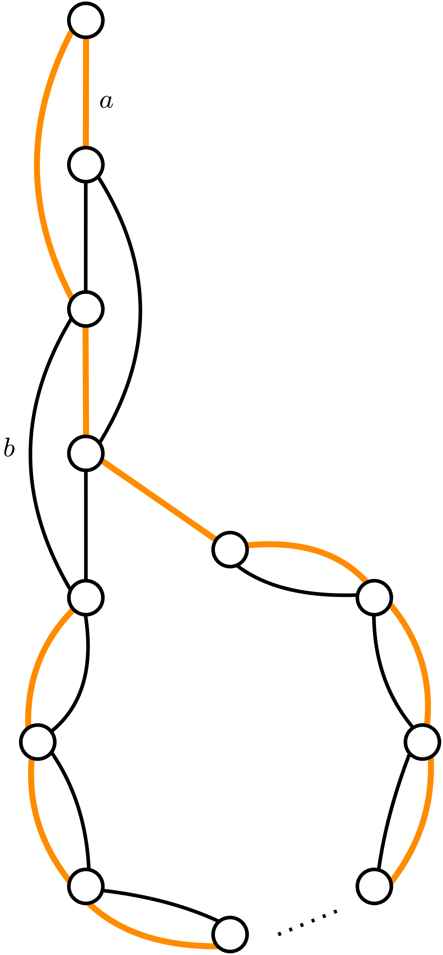
(a)

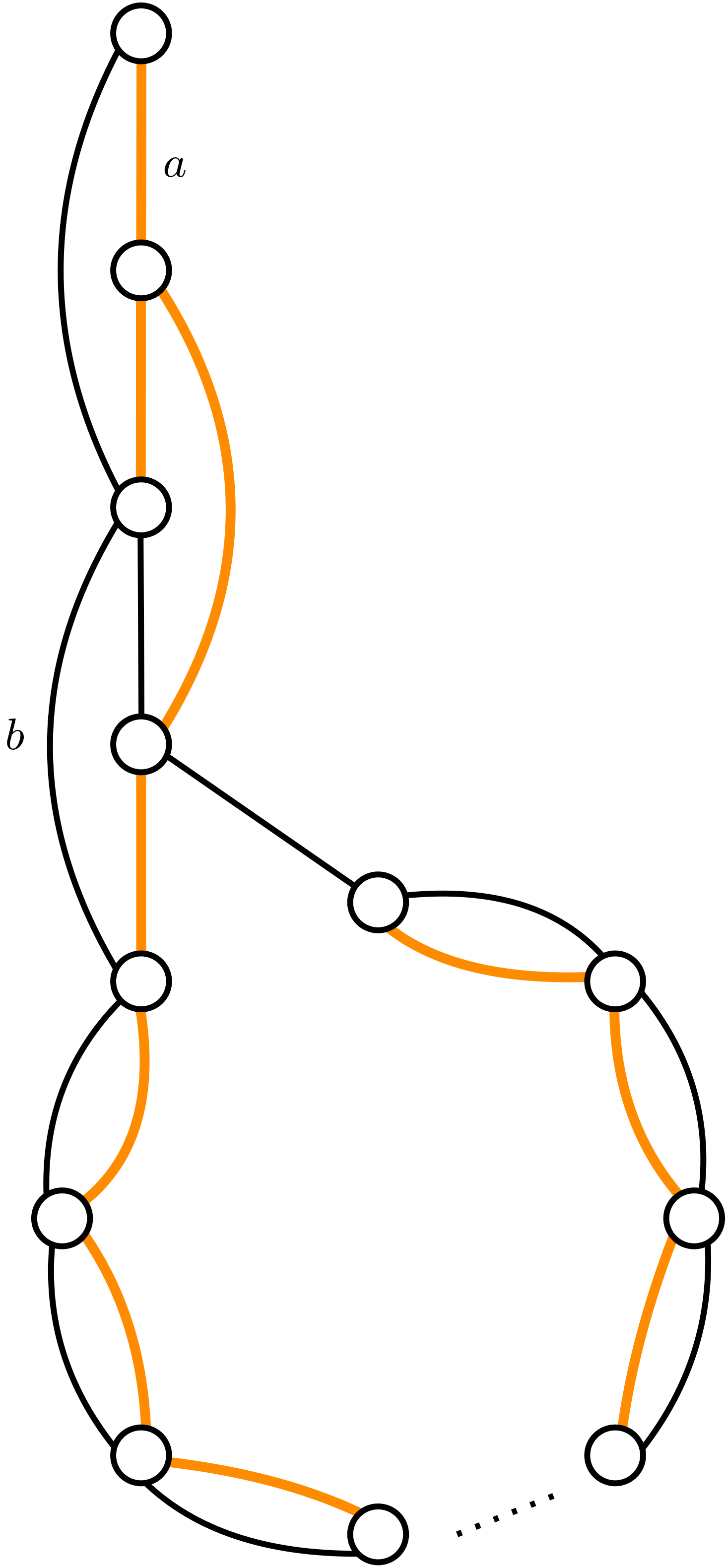
(b)

Figure 1: The graph with two trees of the tree-packing colored. Observe that all edges are packed once in these two trees except for $a$, which is packed twice, and $b$ which is never packed.

We generalize this result for any even $\lambda$, by copying every edge in the above construction $\lambda/2$ times and packing trees on each copy in parallel. For more details, we refer to Section 4.

1.4.4 Existence of Small Greedy Tree-Packing

Our last technical contribution is Section 1.3, showing that there exists a small tree-packing. We first consider the case that $\ell^{*}(e)=1/\Phi$ for every edge $e\in E$. The proof is rather simple, and based on Kaiser’s [Kai12] elegant proof of the tree-packing theorem. This is the theorem initially proved by Tutte [Tut61] and Nash-Williams [NW61] that shows that $\Phi$ (in our notation) is well defined. Another phrasing is as follows: a graph $G$ contains $k$ pairwise disjoint spanning trees if and only if for every partition $\mathcal{P}$ of $V(G)$, the graph $G/\mathcal{P}$ has at least $k(|\mathcal{P}|-1)$ edges. We generalize this to $k$ trees + 1 forest and show that extending this forest to an arbitrary spanning tree gives the required packing.

Next, we use the ideal load decomposition to generalize this to any graph. The trees in our packing are simply unions of the trees on each component. For more details, see Section 5.

2 Min-Cut

In this section, we reexamine the relation between min-cut and tree-packing. The main technical contribution is the following theorem.

*

Thorup [Tho07] showed that if $|\mathcal{T}|=\Omega(\lambda^{7}\log^{3}m)$, then some $T\in\mathcal{T}$ $1$-respects a min-cut. With this new result, we significantly decrease the number of trees we need to pack, leading to a significant speed-up.

This section is organized as follows. In Section 2.1, we give a proof of Section 1.3. In LABEL:sc:trival_cuts, we show how to estimate the trivial cuts of part 2 in Section 1.3 efficiently. In LABEL:sc:TP_recourse, we show how to decrease the recourse in the tree-packing, which leads to a faster running time. In LABEL:sc:mincut_par, we provide our dynamic min-cut algorithm for bounded $\lambda$. And finally, in LABEL:sc:mincut_gen, we provide our dynamic min-cut algorithm for general $\lambda$.

Preliminaries.

Before we move on to the proof of Section 1.3, we first make the theorem statement more precise, and we make the notation more concise.

For some set of edges $E^{\prime}\subseteq E$, we denote $G/E^{\prime}$ for the graph where we contract all edges in $E^{\prime}$. Suppose $uv\in E\setminus E^{\prime}$ and $u$ and $v$ are contracted in $G/E^{\prime}$, then we keep $uv$ as a self-loop in $G/E^{\prime}$. Such edges count twice towards the degree of the corresponding vertex in $G/E^{\prime}$.

Let $E_{\circ a}^{*}:=\{e\in E:\ell^{*}(e)\circ a\}$ and $E_{\circ a}^{\mathcal{T}}:=\{e\in E:\ell^{\mathcal{T}}(e)\circ a\}$ for $\circ\in\{\geq,>,\leq<,=\}$. Further let $G_{a}:=G/E^{\mathcal{T}}_{<a}$. Then in our new notation, part 2 of Section 1.3 corresponds to a trivial cut in $G_{a}=G/E^{\mathcal{T}}_{<a}$ for $a=\tfrac{2}{\lambda}-\tfrac{3}{8\lambda^{2}}$.

Let $\mathcal{M}\mathcal{C}\subseteq E$ denote the set of all edges that are contained in at least one min-cut. And let $\overline{a}$ denote the largest value in $\mathbb{R}$ such that $E^{*}_{\geq\overline{a}}\supseteq\mathcal{M}\mathcal{C}$.

We recall the definition of $\Phi$.

Lemma 1 ([NW61, Tut61]).

We have

$$\Phi_{G}:=\max_{\mathcal{T}}\rm{pack\_val}(\mathcal{T})=\min_{\mathcal{P}}\rm{part\_val}(\mathcal{P}).$$

We will repeatedly use the following simple lemma concerning $\Phi$ and the min-cut $\lambda$. We include a proof for completeness.

Lemma 2 ([Kar00]).

$\lambda/2<\Phi\leq\lambda$.

Proof.

We recall that $\Phi=\min_{\mathcal{P}}\tfrac{|E(G/\mathcal{P})|}{|\mathcal{P}|-1}$, this immediately gives that

$$\Phi\leq\min_{\mathcal{P}=\{A,B\}}\frac{|E(A,B)|}{2-1}=\lambda.$$

Now consider an arbitrary partition $\mathcal{P}$. We note that $2\tfrac{|E(G/\mathcal{P})|}{|\mathcal{P}|}$ is the average value of a trivial cut in $G/\mathcal{P}$. Since this corresponds to a cut in $G$, we get $2\tfrac{|E(G/\mathcal{P})|}{|\mathcal{P}|}\geq\lambda$. Now we see

$$\Phi\geq\frac{|E(G/\mathcal{P})|}{|\mathcal{P}|-1}>\frac{|E(G/\mathcal{P})|}{|\mathcal{P}|}\geq\lambda/2.\qed$$

We have the following lemma showing that a sufficiently large greedy tree-packing approximates the ideal packing, introduced in Section 1.3, well.

Lemma 3 ([Tho07]).

A greedy tree-packing $\mathcal{T}$ with $|\mathcal{T}|\geq 6\lambda\log m/\eta^{2}$ trees, for $\eta<2$, satisfies

$$|\ell^{\mathcal{T}}(e)-\ell^{*}(e)|\leq\eta/\lambda,$$

for all $e\in E$.

2.1 A Proof of Theorem 1.3

Let us first briefly discuss the intuition behind the proof. We start by using reasoning similar to arguments appearing in Thorup [Tho07] to show that if some edge $e^{\prime}\in\mathcal{M}\mathcal{C}$ has $\ell^{*}(e^{\prime})$ small enough, then any min-cut containing $e^{\prime}$ will be crossed once by some tree even if we only pack a relatively small amount of trees. This follows from the observation that if

$$\sum_{e\in C}\ell^{\mathcal{T}}(e)<2$$

for some cut $C$, then some tree crosses $C$ at most once. Indeed, the average number of times $C$ is crossed by a tree is given by

$$\frac{1}{|\mathcal{T}|}\sum_{e\in C}L^{\mathcal{T}}(e)=\sum_{e\in C}\ell^{\mathcal{T}}(e)$$

and at least one tree will cross $C$ at most the average number of times. Hence, if $\ell^{*}(e^{\prime})$ is small enough, i.e., far enough below $\frac{2}{\lambda}$, then it is sufficient to pack $O(\lambda^{3}\log m)$ trees in order to concentrate $\sum_{e\in C}\ell^{\mathcal{T}}(e)$ below $2$. It is important to note here that in order to get this dependency on $\lambda$ one has to use the fact that many of the edges in $C$ will have $\ell^{*}$ values sufficiently far below $\frac{2}{\lambda}$.

From here on, our argument goes in a completely different direction compared to those of Thorup. The starting point for the second part of Section 1.3 is that we may assume $\overline{a}$ is sufficiently close to $\tfrac{2}{\lambda}$. We first use this to show that for an appropriate value $\hat{a}$ only slightly smaller than $\overline{a}$, the graph $G/E^{*}_{<\hat{a}}$ must contain trivial min-cuts. To show this we may assume this is not the case for contradiction, and then count the edges of the graph in two different ways: once using the $\ell^{*}$ values and once by summing the degrees. This then yields a contradiction since $\hat{a}^{-1}$ is sufficiently smaller than $\tfrac{\lambda+1}{2}$.

Next we exploit the fact that if $\ell^{*}(e)<\overline{a}$, then $e$ is not in any min-cut by construction. We focus on an arbitrary trivial min-cut $X$ of $G/E^{*}_{<\hat{a}}$. The remaining part of the proof then boils down to showing that $\Phi_{G[X]}$ is sufficiently large. To do so, we formulate an optimization problem which lower bounds the value $\Phi_{G[X]}$ can take, and then show that the solution to the optimization problem is large enough. To do so, we heavily exploit that no edge in $G[X]$ belongs to a min-cut, and so only very few trivial cuts of any partition of $G[X]$ can deviate from having degree at least $\lambda+1$.

As outlined above, we begin by showing that we must have some $1$-respecting cut if $\overline{a}$ is sufficiently far from $\tfrac{\lambda}{2}$.

Lemma 4.

If $\overline{a}\leq\tfrac{2}{\lambda}-\tfrac{1}{c\lambda^{2}}+\tfrac{1}{\gamma\lambda^{2}}$ with $\gamma\geq 4c$ then 1 holds.

Proof.

By assumption there exists some $e^{\prime}\in\mathcal{M}\mathcal{C}$ such that $\ell^{*}(e^{\prime})=\overline{a}$. Now pick any min-cut $C=(A,B)$ containing $e^{\prime}$ and fix it for the remainder of the proof. We will first show that $|E^{*}_{=\overline{a}}\cap C|\geq\tfrac{\lambda}{2}$. Indeed, consider the graph $G/E^{*}_{<\overline{a}}$. Since $C$ separates the endpoints of $e^{\prime}$ (or $C-e^{\prime}$ is a smaller cut), it must be that $C$ separates the endpoints of $e^{\prime}$ in $G[E^{*}_{=\overline{a}}]$. By applying Lemma 2 twice, we see that $\Phi_{(G/E^{*}_{<\overline{a}})[E^{*}_{=\overline{a}}]}=\overline{a}\geq\tfrac{\lambda}{2}$, and consequently that the smallest cut in $(G/E^{*}_{<\overline{a}})[E^{*}_{=\overline{a}}]$ separating the endpoints of $e^{\prime}$ has size at least $\tfrac{\lambda}{2}$. Hence, it must be that $|E^{*}_{=\overline{a}}\cap C|\geq\tfrac{\lambda}{2}$.

Following the earlier discussion, we now want to argue that

$$\sum_{e\in C}\ell^{\mathcal{T}}(e)<2.$$

This follows from the fact that we pack $|\mathcal{T}|=\Omega(\tfrac{\lambda\log m}{\varepsilon^{2}})$ trees, and so we achieve concentration $\varepsilon<\tfrac{3}{8c\lambda}$ and thus we can write:

$$\sum_{e\in C}\ell^{\mathcal{T}}(e)\leq\sum_{e\in C}\ell^{*}(e)+\lambda\cdot{}\frac{\varepsilon}{\lambda}\leq\lambda\cdot{}\frac{2}{\lambda}-\frac{\lambda}{2}(\frac{1}{c\lambda^{2}}-\frac{1}{\gamma\lambda^{2}})+\varepsilon\leq 2-\frac{3}{8c\lambda}+\varepsilon<2,$$

which per the previous discussion implies that 1 holds. ∎

Following the proof out-line in the beginning of this section, we next show that if $\overline{a}$ is greater than or equal to the cut-off value of $\tfrac{2}{\lambda}-\tfrac{1}{c\lambda^{2}}+\tfrac{1}{\gamma\lambda^{2}}$, then it is sufficiently close to $\tfrac{2}{\lambda}$ for 2 to hold. We begin by showing that $G/E^{*}_{<\overline{a}}$ must contain at least one trivial min-cut that corresponds to a min-cut of $G$.

Lemma 5.

Suppose that $\gamma\geq 4c>4$, then $G/E^{*}_{<\tfrac{2}{\lambda}-\tfrac{1}{c\lambda^{2}}+\tfrac{1}{\gamma\lambda^{2}}}$ contains at least one trivial min-cut that corresponds to a min-cut of $G$.

Proof.

As hinted to earlier, we will assume that this is not the case for contradiction. We will then count the edges of $G^{\prime}=G/E^{*}_{<\tfrac{2}{\lambda}-\tfrac{1}{c\lambda^{2}}+\tfrac{1}{\gamma\lambda^{2}}}$ twice to reach the contradiction. To do so, let $\mathcal{P}_{0}$ be the packing for $G$ with $\rm{pack\_val}(\mathcal{P}_{0})=\Phi$. Next, we recurse on the subgraphs $G[S]$ for each $S\in\mathcal{P}_{0}$. We write the total decomposition as $P_{i}$ the packing on $G[S_{i}]$, where each $S_{i}\in P_{j}$ for some $j<i$, for $i\in\mathcal{I}$ for some index set $\mathcal{I}$. We are only interested in parts of the decomposition, and so we will only recurse on $S_{i}\in P_{j}$ if $\Phi_{G[S_{i}]}\leq(\tfrac{2}{\lambda}-\tfrac{1}{c\lambda^{2}}+\tfrac{1}{\gamma\lambda^{2}})^{-1}$.

Now we have the containment:

$$E^{*}_{\geq\frac{2}{\lambda}-\frac{1}{c\lambda^{2}}+\frac{1}{\gamma\lambda^{2}}}\subset\bigcup_{i\in\mathcal{I}}E(G[S_{i}]/\mathcal{P}_{i}).$$

Indeed, any edge in $E^{*}_{\geq\frac{2}{\lambda}-\frac{1}{c\lambda^{2}}+\frac{1}{\gamma\lambda^{2}}}$ will be included since by Lemma 1, we have that $\Phi_{G[S]}=(\max_{e\in G[S_{i}]}\ell^{*}(e))^{-1}$, and so the recursion will not terminate until every edge in $E^{*}_{\geq\frac{2}{\lambda}-\frac{1}{c\lambda^{2}}+\frac{1}{\gamma\lambda^{2}}}$ belongs to some subgraph. In fact, the containment is an equality. Next, we have

$$|E^{*}_{\geq\frac{2}{\lambda}-\frac{1}{c\lambda^{2}}+\frac{1}{\gamma\lambda^{2}}}| \leq\sum_{i\in\mathcal{I}}|E(G[S_{i}]/\mathcal{P}_{i})|$$

$$\leq\sum_{i\in\mathcal{I}}\Phi_{i}(|V_{i}|-1)$$

$$\leq(\frac{2}{\lambda}-\frac{1}{c\lambda^{2}}+\frac{1}{\gamma\lambda^{2}})^{-1}\sum_{i\in\mathcal{I}}(|V_{i}|-1),$$

where $\Phi_{i}$ is the packing value of $\mathcal{P}_{i}$, and $V_{i}=V(G[S_{i}]/\mathcal{P}_{i})$. Next, we show that

$$\sum_{i\in\mathcal{I}}(|V_{i}|-1)\leq|V(G^{\prime})|-1.$$

We divide $\mathcal{I}$ in different depths of recursion: let $\mathcal{I}_{j}$ be such that for $i\in\mathcal{I}_{j}$ we have $S_{i}$ in recursion depth $j$ (i.e., it is in $j$ partitions before). For ease of notation, we let a singleton cluster $\{v\}$ again partition into $\{v\}$. This has no effect on the sum over $|V_{i}|-1$, but ensures that all vertices make it to the lowest depth. Let $r$ be the total recursion depth. With this notation, we can write for $0\leq j<r$

$$\sum\limits_{i\in I_{j}}|V_{i}|=|I_{j+1}|$$

since we must recurse exactly once on each vertex in $V_{i}$ in the next level. Let the partition $\hat{\mathcal{P}}$ of $G$ be obtained by letting $S\in\hat{\mathcal{P}}$ if and only if $S\in P_{i}$ for some $i\in I_{r}$. Then, similarly to above, the introduced notation implies that

$$\sum\limits_{i\in I_{r}}|V_{i}|=|V(G/\hat{\mathcal{P}})|.$$

We have $E^{*}_{\geq\frac{2}{\lambda}-\frac{1}{c\lambda^{2}}+\frac{1}{\gamma\lambda^{2}}}\subset E(G/\hat{\mathcal{P}})$ by before. Thus, we note that any edge contracted in $G/\hat{\mathcal{P}}$ is also contracted in $G^{\prime}$, and therefore we have $|V(G/\hat{\mathcal{P}})|\leq|V(G^{\prime})|$. Indeed, contracting an edge can never increase the size of the vertex set. Finally, we can write

$$\sum_{i\in\mathcal{I}}(|V_{i}|-1) =\sum_{j=0}^{r}\sum_{i\in\mathcal{I}_{j}}(|V_{i}|-1)$$

$$=\sum_{j=0}^{r}\left(\sum_{i\in\mathcal{I}_{j}}|V_{i}|\right)-|I_{j}|$$

$$=|V(G/\hat{\mathcal{P}})|-|I_{r}|+\sum_{j=0}^{r-1}|\mathcal{I}_{j+1}|-|\mathcal{I}_{j}|$$

$$=|V(G/\hat{\mathcal{P}})|-|I_{0}|$$

$$\leq|V(G^{\prime})|-1.$$

Now we upper bound as follows:

$$|E^{*}_{\geq\frac{2}{\lambda}-\frac{1}{c\lambda^{2}}+\frac{1}{\gamma\lambda^{2}}}| \leq\left(\frac{2}{\lambda}-\frac{1}{c\lambda^{2}}+\frac{1}{\gamma\lambda^{2}}\right)^{-1}\sum_{i\in\mathcal{I}}(|V_{i}|-1)$$

$$\leq\left(\frac{2}{\lambda}-\frac{1}{c\lambda^{2}}\right)^{-1}(|V(G^{\prime})|-1)$$

$$\leq\frac{\frac{\lambda}{2}}{1-\frac{1}{2c\lambda}}(|V(G^{\prime})|-1)$$

$$\leq\frac{\lambda}{2}\left(1+\frac{1}{c\lambda}\right)(|V(G^{\prime})|-1)$$

$$\leq\left(\frac{\lambda}{2}+\frac{1}{2c}\right)(|V(G^{\prime})|-1),$$

where we used the well-known fact that $\tfrac{1}{1-x}\leq 1+2x$ if $x<1$.

To reach a contradiction, we let $\mathcal{P}$ be the final partition obtained in the above procedure and and apply the classical hand-shaking lemma to obtain:

$$|E^{*}_{\geq\frac{2}{\lambda}-\frac{1}{c\lambda^{2}}+\frac{1}{\gamma\lambda^{2}}}|=\frac{1}{2}\sum\limits_{X\in\mathcal{P}}d_{G^{\prime}}(X)\geq\frac{\lambda+1}{2}|V(G^{\prime})|,$$

which is a contradiction for $c>1$. Here we used the assumption that $G^{\prime}$ contains no trivial cut of size $\lambda$. Note that a cut of $G^{\prime}$ corresponds to a cut in $G$ containing the exact same edges. ∎

Finally, we show that if one was to recurse the idealized load decomposition on a partition in $G/E^{*}_{<\tfrac{2}{\lambda}-\tfrac{1}{c\lambda^{2}}+\tfrac{1}{\gamma\lambda^{2}}}$, then the recursive call on a trivial cut will produce a new set $S$ for which $\Phi_{G[S]}$ is sufficiently far away from $\overline{a}$ to establish a separation.

Lemma 6.

Suppose $\overline{a}\geq\tfrac{2}{\lambda}-\tfrac{1}{c\lambda^{2}}+\tfrac{1}{\gamma\lambda^{2}}$, and let $\mathcal{P}$ be the partition induced in $G/E^{*}_{<\frac{2}{\lambda}-\frac{1}{c\lambda^{2}}+\frac{1}{\gamma\lambda^{2}}}$, and let $S\in\mathcal{P}$ be any trivial min-cut in this partition. Then we have

$$\Phi_{G[S]}\geq\frac{\lambda}{2}+\frac{1}{2}.$$

Proof.

We will exploit the fact that no edge belonging to $E(G[S])$ is contained in any min-cut. We consider the minimum partition of $G[S]$, call it $\mathcal{P}_{S}$, and let $\tilde{G}=G[S]/\mathcal{P}_{S}$. Then it must be the case that any vertex of degree $d\leq\lambda$ in $\tilde{G}$ is incident to at least $\lambda+1-d$ edges in $G/E^{*}_{<\frac{2}{\lambda}-\frac{1}{c\lambda^{2}}+\frac{1}{\gamma\lambda^{2}}}$. Indeed, otherwise the edge belongs to some min-cut in $G$, which contradicts the choice of $\overline{a}$. It now follows that any choice of $\tilde{G}$ with $k$ vertices must induce a feasible solution to the following optimization problem with objective value $\Phi_{\tilde{G}}$:

3 Arboricity

In this section, we first show a structural result: a relation between the fractional arboricity and the ideal relative loads of a tree-packing, see Section 3.1. We then give a deterministic dynamic algorithm, that is efficient for small values of $\alpha$, see Section 3.2. For simple graphs, we can combine this with the state of the art for densest subgraph approximation, see Section 3.3. For multi-graphs, we need to downsample the high $\alpha$ regime to low $\alpha$ regime. While this is relatively straight-forward against an oblivious adversary (Section 3.4), it is much more involved against an adaptive adversary (Section 3.5).

3.1 Structural Result

The idea is to show that $(\min\ell^{*}(e))^{-1}=\alpha(G)$. Then we can estimate $\alpha(G)$ by simply taking $\alpha_{\rm{est}}=(\min\ell(e))^{-1}$, with $\ell$ some good approximation of $\ell^{*}$. For the integral arboricity, $\lceil\alpha\rceil$, a similar result follows already from [Tut61, NW61, NW64]. We achieve this, more nuanced result by using the language of ideal load decompositions from [Tho07]. In particular, we use the following observation. We provide a proof for completeness.

Observation 7 ([Tho07]).

For each $S\in\mathcal{P}^{*}$, we have $\Phi_{G[S]}\geq\Phi$.

Proof.

We will prove this by contradiction. Suppose $\mathcal{P}$ is a partition of $S$ such that $\rm{part\_val}(\mathcal{P})<\Phi$. Let $\mathcal{P}^{\prime}=(\mathcal{P}^{*}\setminus\{S\})\cup\mathcal{P}$ be a partition of $V$, then we see that

$$\rm{part\_val}(\mathcal{P}^{\prime})=\frac{|E(G/\mathcal{P}^{\prime})|}{|\mathcal{P}^{\prime}|-1}=\frac{|E(G/\mathcal{P}^{*})|+|E(G[S]/\mathcal{P})|}{|\mathcal{P}^{*}|-1+|\mathcal{P}|-1}<\frac{\Phi(|\mathcal{P}^{*}|-1)+\Phi(|\mathcal{P}|-1)}{|\mathcal{P}^{*}|-1+|\mathcal{P}|-1}=\Phi,$$

using that $\frac{|E(G/\mathcal{P}^{*})|}{|\mathcal{P}^{*}|-1}=\Phi$ and $\frac{|E(G[S]/\mathcal{P})|}{|\mathcal{P}|-1}=\rm{part\_val}(\mathcal{P})<\Phi$ ∎

Now we can show the main result.

Theorem 8.

Let $G=(V,E)$ be an undirected, unweighted (multi-)graph, then

$$\alpha(G)=\frac{1}{\min_{e\in E}\ell^{*}(e)}.$$

Proof.

We start by showing $\alpha(G)\geq(\min_{e\in E}\ell^{*}(e))^{-1}$. We note that $(\min_{e\in E}\ell^{*}(e))^{-1}=\max_{i}\Phi_{i}$, ranging over all partitions appearing in the ideal partitioning. Denote the graph where this is maximized by $G^{*}$, and its vertex set by $X$. By 7, we have that it does not further partition, hence $\mathcal{P}^{*}=X$, so $G^{*}/\mathcal{P}^{*}=G^{*}$ and $G^{*}=G[X]$. Now we can conclude

$$(\min_{e\in E}\ell^{*}(e))^{-1} =\max_{i}\Phi_{i}=\frac{|E(G^{*}/\mathcal{P}^{*})|}{|\mathcal{P}^{*}|-1}=\frac{|E(G[X])|}{|X|-1}$$

$$\leq\max_{Y\subseteq V}\frac{|E(G[Y])|}{|Y|-1}=\alpha(G).$$

Next, we show that $\alpha(G)\leq(\min_{e\in E}\ell^{*}(e))^{-1}$. Let $Y\subseteq V$ be any subset. We will show that

$$\frac{|E(Y)|}{|Y|-1}\leq(\min_{e\in E}\ell^{*}(e))^{-1}.$$

Hence $\alpha(G)=\max_{Y\subseteq V}\frac{E(Y)}{|Y|-1}\leq(\min_{e\in E}\ell^{*}(e))^{-1}.$

The arguments we use here are very similar to the proof of Lemma 5, where we present them with more detail. We inspect the definition of ideal relative loads: let $\mathcal{P}_{0}$ the packing for $G$ with $\rm{pack\_val}(\mathcal{P}_{0})=\Phi$. Now we recurse on the subgraphs $G[S]$ for each $S\in\mathcal{P}_{0}$. We write the total decomposition as $P_{i}$ the packing on $G[S_{i}]$, where each $S_{i}\in P_{j}$ for some $j<i$, for $i\in\mathcal{I}$ for some index set $\mathcal{I}$. Now we have the disjoint union:

$$E(G)=\bigcup_{i\in\mathcal{I}}E(G[S_{i}]/\mathcal{P}_{i}).$$

So in particular we have

$$|E(Y)|=\sum_{i\in\mathcal{I}}|E(Y)\cap E(G[S_{i}]/\mathcal{P}_{i})|\leq\sum_{i\in\mathcal{I}}\Phi_{i}(|V_{Y,i}|-1),$$

where $\Phi_{i}$ is the packing value of $\mathcal{P}_{i}$, and $V_{Y,i}=Y\cap V(G[S_{i}]/\mathcal{P}_{i})$. Note that the inequality follows from the fact that if $E(Y)\cap E(G[S_{i}]/\mathcal{P}_{i})$ contains more than $\Phi_{i}(|V_{Y,i}|-1)$ edges, then one can contract all such edges to get a new partition with at most $|V_{Y,i}|-1$ fewer vertices but more than $\Phi_{i}(|V_{Y,i}|-1)$ fewer edges, which contradicts the choice of $\Phi_{i}$. Next, we prove that

$$\sum_{i\in\mathcal{I}}(|V_{Y,i}|-1)=|Y|-1.$$

We divide $\mathcal{I}$ in different depths of recursion: let $\mathcal{I}_{j}$ be such that for $i\in\mathcal{I}_{j}$ we have $S_{i}\cap Y$ in recursion depth $j$ (i.e., it is in $j$ partitions before). Let $r$ be the total recursion depth. Then we can write

$$\sum_{i\in\mathcal{I}}(|V_{Y,i})|-1) =\sum_{j=0}^{r}\sum_{i\in\mathcal{I}_{j}}(|V_{Y,i}|-1)$$

$$=\sum_{j=0}^{r}\left(\sum_{i\in\mathcal{I}_{j}}|V_{Y,i}|\right)-|I_{j}|$$

$$=\sum_{j=1}^{r}|\mathcal{I}_{j}|-|\mathcal{I}_{j-1}|$$

$$=|\mathcal{I}_{r}|-|\mathcal{I}_{0}|$$

$$=|Y|-1.$$

Now we use this as follows:

$$\frac{|E(Y)|}{|Y|-1} \leq\frac{\sum_{i\in\mathcal{I}}\Phi_{i}(|V_{Y,i}|-1)}{|Y|-1}$$

$$\leq\left(\max_{i\in\mathcal{I}}\Phi_{i}\right)\frac{\sum_{i\in\mathcal{I}}|V_{Y,i}|-1}{|Y|-1}$$

$$=\max_{i\in\mathcal{I}}\Phi_{i}$$

$$=(\min_{e\in E}\ell^{*}(e))^{-1},$$

where the last equality holds by definition of $\ell^{*}$.

∎

Next, we use the fact that a greedy tree-packing approximates an ideal packing well to give an approximation of the fractional arboricity.

Lemma 9.

A greedy tree-packing $\mathcal{T}$ with $|\mathcal{T}|\geq\tfrac{24\alpha^{2}\log m}{\varepsilon^{2}}$ trees satisfies, for $\varepsilon\in(0,1)$,

$$\left|\frac{1}{\min_{e\in E}\ell^{\mathcal{T}}(e)}-\alpha\right|\leq\varepsilon\alpha.$$

Proof.

The tree-packing $\mathcal{T}$ contains

$$\frac{24\alpha^{2}\log m}{\varepsilon^{2}}\geq\frac{6(1+\varepsilon)^{2}\alpha^{2}\log m}{\lambda\varepsilon^{2}}=\frac{6\log m\lambda}{\left(\frac{\lambda}{\alpha(1+\varepsilon)}\varepsilon\right)^{2}}$$

trees. We note that $\tfrac{\lambda}{\alpha(1+\varepsilon)}\varepsilon\leq\tfrac{\lambda}{\alpha}\varepsilon\leq\varepsilon<1$, so we can apply Lemma 3 with $\eta=\tfrac{\lambda}{\alpha(1+\varepsilon)}\varepsilon$ to obtain

$$\left|\min_{e\in E}\ell^{\mathcal{T}}(e)-\min_{e\in E}\ell^{*}(e)\right|\leq\frac{\varepsilon}{\alpha(1+\varepsilon)}.$$

Now we see that

$$\frac{1}{\min_{e\in E}\ell^{\mathcal{T}}(e)}-\alpha \leq\frac{1}{\min_{e\in E}\ell^{*}(e)-\frac{\varepsilon}{\alpha(1+\varepsilon)}}-\alpha$$

$$=\frac{1}{\frac{1}{\alpha}-\frac{\varepsilon}{\alpha(1+\varepsilon)}}-\alpha$$

$$=\left(\frac{1}{\frac{1+\varepsilon}{1+\varepsilon}-\frac{\varepsilon}{(1+\varepsilon)}}-1\right)\alpha$$

$$=\varepsilon\alpha.$$

The proof that $\alpha-\tfrac{1}{\min_{e\in E}\ell^{\mathcal{T}}(e)}\leq\varepsilon\alpha$ is analogous. ∎

3.2 Dynamic Algorithm for Bounded $\alpha$

In this section, we show how to dynamically maintain the estimate $\tfrac{1}{\min_{e\in E}\ell^{\mathcal{T}}(e)}$, giving us the arboricity estimate. We start with a warm-up giving the result almost directly by plugging in a deterministic minimum spanning tree algorithm.

3.2.1 Warm-Up

Lemma 10.

There exists a deterministic dynamic algorithm, that given an unweighted, undirected (multi-)graph $G=(V,E)$, maintains a $(1+\varepsilon)$-approximation of the fractional arboricity $\alpha$ when $\alpha\leq\alpha_{\max}$ in $O(\alpha_{\max}^{4}\log^{6}m/\varepsilon^{4})$ amortized update time or a Las Vegas algorithm with $O(\alpha_{\max}^{4}m^{o(1)}/\varepsilon^{4})$ worst-case update time.

Proof.

By Lemma 9, all we need to do is maintain $\Theta(\tfrac{\alpha_{\max}^{2}\log m}{\varepsilon^{2}})$ greedy spanning trees, and then maintain the minimum over $\ell^{\mathcal{T}}(e)$. The latter can simply be done by maintaining a min-heap, which has an update time of $O(\log m)$.

For the former, we note that any edge insertion or deletion can lead to overall $O\left(\left(\tfrac{\alpha_{\max}^{2}\log m}{\varepsilon^{2}}\right)^{2}\right)$ updates to the spanning trees [TK00]. We can use a deterministic dynamic minimum spanning tree algorithm with

• $O(\log^{4}m)$ amortized update time deterministically [HLT01]; or

• $m^{o(1)}$ worst-case update time (Las Vegas algorithm) [NSW17].

Multiplying these update times with the number of spanning tree updates per insertion/deletion gives the result. Note that both subsume the $O(\log m)$ update time for maintaining the min-heap. ∎

3.2.2 Recourse in Tree-Packing

Next, we show how we can bound the recourse in the tree-packing to shave a factor $\alpha_{\max}$. This is similar to LABEL:lm:TP_recourse_impr, but has additional complications: to bound the recourse we need to guarantee a high min-cut, and we need to show we can keep an artificially high min-cut in a graph with certain arboricity. Note that there are even disconnected graphs with linear arboricity, so this is a non-trivial adaptation.

*

Proof.

By Lemma 9, all we need to do is maintain $\Theta(\tfrac{\alpha^{2}\log m}{\lambda\varepsilon^{2}})$ greedy spanning trees, and then maintain the minimum over $\ell^{\mathcal{T}}(e)$. As opposed to Lemma 10, we do not do this once with $\alpha_{\max}$, but keep $\log\alpha_{\max}$ copies corresponding to different values of $\alpha$. The goal is to establish $O(|\mathcal{T}|^{2}/\alpha)$ recourse instead of the trivial $O(|\mathcal{T}|^{2})$ recourse. We do this by utilizing that the recourse is $O(|\mathcal{T}|^{2}/\lambda)$, and artificially increase the min-cut to $\Theta(\alpha)$. This simultaneously means we only need to maintain $|\mathcal{T}|=\Theta(\tfrac{\alpha\log m}{\varepsilon^{2}})$ greedy spanning trees.

To be precise, we maintain tree-packings $\mathcal{T}_{1},\mathcal{T}_{2},\dots,\mathcal{T}_{\log\lambda_{\max}}$, where $|\mathcal{T}_{i}|=O(2^{i}\log m/\varepsilon^{2})$. We only need the packing $\mathcal{T}_{i}$ when $\alpha\in[2^{i},2^{i+1})$. If $\alpha\notin[2^{i},2^{i+1})$, we still need the update times to hold, but we do not need the output to be correct. Each tree-packing $\mathcal{T}_{i}$ is the tree-packing of some graph $G_{i}$, where we show that $\alpha=\alpha(G_{i})$ if $\alpha\in[2^{i},2^{i+1})$. As opposed to LABEL:lm:TP_recourse_impr, we do not guarantee the stronger statement that $G_{i}=G$ in this case.

First, we assume that $G_{i}$ initially has min-cut $\lambda\geq 2^{i-1}$. This means that initially $\ell^{\mathcal{T}_{i}}(e)\leq\ell^{*}(e)+\varepsilon/2^{i-1}\leq 1/\Phi_{G_{i}}+1/2^{i-1}\leq 2/2^{i-1}+1/2^{i-1}=O(1/2^{i})$, using Lemma 3 with $\eta=1$. Throughout the updates, we keep an edge $e$ as a virtual edge if deleting $e$ would cause any edge $e^{\prime}$ to reach $\ell^{\mathcal{T}_{i}}(e^{\prime})\geq 16/2^{i}$. By the same arguments as in LABEL:lm:TP_recourse_impr, this gives amortized recourse $O(|\mathcal{T}_{i}|^{2}/2^{i})$ for $\mathcal{T}_{i}$. We delete a virtual edge $e$ if $\ell^{\mathcal{T}_{i}}(e)<8/2^{i}$ after some update. This cannot lead to the load of any other edge rising above $16/2^{i}$, see Claim 1 in LABEL:lm:TP_recourse_impr. Since any virtual edge was inserted as a real edge at some point, we can amortize the cost of this deletion. Next, we show that the virtual edges do not interfere with the arboricity if $2^{i}\leq\alpha$, in which case $8/2^{i}\geq 8/\alpha$. We do this with two claims.

• If $\ell^{\mathcal{T}_{i}}(e)\geq 8/\alpha$ then $\ell^{*}(e)\geq 4/\alpha$.
  Proof. By Lemma 3 we have $\ell^{*}(e)\geq\ell^{\mathcal{T}_{i}}(e)-\varepsilon/\alpha\geq 4/\alpha$.

• Let $\ell^{*}(e)>\tfrac{1}{\alpha}$ and let $S^{*}\subseteq V$ be such that $\alpha=\tfrac{|E(S^{*})|}{|S^{*}|-1}$. Then $e\not\subset S^{*}$.
  Proof. Consider the partition induced by the last level of the ideal load decomposition $\mathcal{P}^{*}$, i.e., the classes of $\mathcal{P}^{*}$ are the connected components induced by edges $f$ with $\ell^{*}(f)=\tfrac{1}{\alpha}$. Note that by arguments similar to Lemma 5 and Theorem 8, we have $1)$ that $e\in E(G/\mathcal{P}^{*})$ and $2)$ that $\frac{|E(G/\mathcal{P}^{*})|}{|\mathcal{P}^{*}|-1}<\alpha$. Now suppose the classes of $\mathcal{P}^{*}$ are $P_{1},\dots,P_{t}$. W.l.o.g., possibly by renumbering, we can assume that $|S^{*}\cap P_{j}|\neq\emptyset$ for all $1\leq j\leq i$ and $|S^{*}\cap P_{j}|=\emptyset$ for all $j>i$. If $i=1$, we are done, so assume $i>1$. Observe first that the graph induced by $P_{1},\dots,P_{i}$ in $G/\mathcal{P}^{*}$ contains strictly less than $\alpha(i-1)$ edges. Indeed, suppose for contradiction this is not so. If $i=t$ then the supposition contradicts $2)$, and if $i<t$, then one would need to contract $P_{1},\dots,P_{i}$ in every level except for the last level of the ideal load decomposition, thus contradicting the choice of $\mathcal{P}^{*}$.

  Finally, we claim that for some $s\in[i]$, we must have $|E(G[S^{*}\cap P_{s}])|>\alpha(|S^{*}\cap P_{s}|-1)$ contradicting that $G$ has arboricity $\alpha$. Indeed, observe that

  $$\alpha=\frac{|E(S^{*})|}{|S^{*}|-1} \leq\frac{|E(P_{1},P_{2},\dots,P_{i})|+\sum_{j=1}^{i}|E(S^{*}\cap P_{j})|}{|S^{*}|-1}$$

  $$=\frac{|E(P_{1},P_{2},\dots,P_{i})|+\sum_{j=1}^{i}|E(S^{*}\cap P_{j})|}{(i-1)+\sum_{j=1}^{i}(|S^{*}\cap P_{j}|-1)}$$

  $$<\frac{\alpha(i-1)+\sum_{j=1}^{i}|E(S^{*}\cap P_{j})|}{(i-1)+\sum_{j=1}^{i}(|S^{*}\cap P_{j}|-1)},$$

  where we used that $|S^{*}|=\sum_{j=1}^{i}|S^{*}\cap P_{j}|=i+\sum_{j=1}^{i}(|S^{*}\cap P_{j}|-1)$. Finally, the claim follows by observing that the final inequality is false if $|E(S^{*}\cap P_{j})|\leq\alpha(|S^{*}\cap P_{j}|-1)$ for all $1\leq j\leq i$.

Combining the two claims above, we see that any edge with $\ell^{\mathcal{T}_{i}}(e)\geq 8/2^{i}\geq 8/\alpha$ is not part of a subgraph for some choice of $S^{*}$ achieving the arboricity. So $\alpha(G_{i})\leq\alpha(G)$. Since $G\subseteq G_{i}$, we also have $\alpha(G)\leq\alpha(G_{i})$, thus we conclude $\alpha(G)=\alpha(G_{i})$. This means that it suffices to approximate the arboricity in $G_{i}$.

Now we discuss an initial initialization step to guarantee that we have $\lambda\geq 2^{i-1}$. We do this by vertex insertions. We initialize all our data structures on a graph with $n$ vertices, but no edges. We add an edge only if both endpoints have degree at least $2^{i-1}$. Note that this corresponds to inserting the vertex with its edges when its degree reaches this boundary. This means we insert at most two vertices at any time. When we insert such a vertex, and it has less than $2^{i-1}$ edges towards the other vertices already present, we add the remainder in virtual edges. This guarantees min-cut $\lambda\geq 2^{i-1}$ at any time. Observe that an edge (or its virtual representative) is added and deleted at most twice.

• If $\deg(v)\leq 2^{i-1}$, then $v\notin S^{*}$ for any $S^{*}\subseteq V$ such that $2^{i}\leq\alpha=\tfrac{|E(S^{*})|}{|S^{*}|-1}$.
  Proof. Let $S^{*}\subseteq V$ be such that $2^{i}\leq\alpha=\tfrac{|E(S^{*})|}{|S^{*}|-1}$, and suppose $v\in S^{*}$

  $$\frac{|E(S^{*}\setminus\{v\})|}{|S^{*}\setminus\{v\}|-1}=\frac{|E(S^{*})|-|E(S,\{v\})|}{|S^{*}|-2}\geq\frac{2^{i}(|S^{*}|-1)-2^{i-1}}{|S^{*}|-2}>2^{i},$$

  which is a contradiction.

Next, we consider the update time: each such vertex insertion takes $O(|\mathcal{T}_{i}|^{2}/2^{i})$ amortized update time. We show that we can perform such a vertex insertion in $O(|\mathcal{T}_{i}|^{2})$ time. Since it required $2^{i-1}$ insertions to reach this degree, this gives the amortized bound. We consider each of the $|\mathcal{T}_{i}|$ trees in the packing and perform all updates simultaneously to it. This consists of the $2^{i-1}$ insertions, plus $O(2^{i-1}\cdot{}|\mathcal{T}_{i}|/2^{i})=O(|\mathcal{T}_{i}|)$ recourse from the earlier trees (since each edge ends up in at most $O(|\mathcal{T}_{i}|/2^{i})$ trees). In total this gives $O(|\mathcal{T}_{i}|(|\mathcal{T}_{i}|+2^{i-1}))=O(|\mathcal{T}_{i}|^{2})$ time.

As before, we use a deterministic dynamic minimum spanning tree algorithm with $O(\log^{4}m)$ amortized update time deterministically [HLT01] for maintaining the trees in each packing. This gives update time $O(2^{i}\log^{6}m/\varepsilon^{4})$ for each $\mathcal{T}_{i}$, hence the update times sum up to $O(\alpha_{\max}\log^{6}m/\varepsilon^{4})$ amortized update time.

The worst-case result is obtained in the same way, with the exception that the insertions cannot be amortized over the edge insertions. Hence the worst-case update time is proportional to $|\mathcal{T}_{i}|^{2}$. Using that we maintain the minimum spanning trees in $n^{o(1)}$ time [NSW17], we obtain the result. ∎

3.3 Dynamic Result for Simple Graphs

We will use the following approximation for the densest subgraph problem, where we say that $\tilde{\rho}$ is a $(1-\varepsilon)$-approximation of $\rho$ when $(1-\varepsilon)\rho\leq\tilde{\rho}\leq\rho$.

Lemma 11 ([SW20, CCHH+24]).

There exists a deterministic dynamic algorithm, that given an unweighted, undirected (multi-)graph $G=(V,E)$, maintains a $(1-\varepsilon)$-approximation of the density $\rho$ in $O(\log^{3}m/\varepsilon^{4})$ amortized update time or $O(\log^{4}m/\varepsilon^{6})$ worst-case update time.

We use this result in the high arboricity regime ($\alpha\geq 1/\varepsilon$), where the density is a good approximation of the fractional arboricity for simple graphs.

*

Proof.

The algorithm is as follows:

• Maintain a fractional arboricity estimate $\tilde{\alpha}$ with $\alpha_{\max}=\Theta(1/\varepsilon)$ using Section 1.2;

• Maintain a $(1-\varepsilon)$-estimate $\tilde{\rho}$ of the densest subgraph using Lemma 11;

• If $\alpha\leq\Theta(1/\varepsilon)$, output $\tilde{\alpha}$, else output $\tilde{\rho}$.

By Section 1.2, we know that $\tilde{\alpha}$ is a $(1+\varepsilon)$-approximation of the fractional arboricity if $\alpha\leq\alpha_{\max}$. We next show that $\tilde{\rho}$ is a $(1+\varepsilon)$-approximation if $\alpha\geq 1/\varepsilon$. Because these ranges overlap, and an update can change the fractional arboricity by at most $1$, we can easily see when we should switch from one estimate to the other.

Note that we always have

$$\tilde{\rho}\leq\rho=\max_{S\subseteq V}\frac{|E(S)|}{|S|}=\frac{|E(S^{*})|}{|S^{*}|}\leq\frac{|E(S^{*})|}{|S^{*}|-1}\leq\max_{S\subseteq V}\frac{|E(S)|}{|S|-1}=\alpha,$$

for some $S^{*}\subseteq V$. Now let $S^{*}$ be such that

$$\max_{S\subseteq V}\frac{|E(S)|}{|S|-1}=\frac{|E(S^{*})|}{|S^{*}|-1}.$$

Using that $G$ is simple, we now have for $\alpha\geq 1/\varepsilon$

$$|S^{*}|\geq\frac{|S^{*}|(|S^{*}|-1)}{|S^{*}|-1}\geq\frac{|E(S^{*})|}{|S^{*}|-1}=\alpha\geq 1/\varepsilon.$$

We use this to see that

$$\alpha-\rho =\frac{|E(S^{*})|}{|S^{*}|-1}-\max_{S\subseteq V}\frac{|E(S)|}{|S|}\leq\frac{|E(S^{*})|}{|S^{*}|-1}-\frac{|E(S^{*})|}{|S^{*}|}$$

$$=|E(S^{*})|\frac{|S^{*}|-(|S^{*}|-1)}{|S^{*}|(|S^{*}|-1)}=\frac{\alpha}{|S^{*}|}\leq\varepsilon\alpha.$$

Rearranging gives us

$$\tilde{\rho}\geq(1-\varepsilon)\rho\geq(1-\varepsilon)^{2}\alpha.$$

Setting $\varepsilon\leftarrow\varepsilon/3$ gives that $\tilde{\rho}$ is a $(1-\varepsilon)$-approximation of the fractional arboricity $\alpha$.

Concerning the update time, we need $O(\log^{6}m/\varepsilon^{5})$ amortized update time for small $\alpha$, and $O(\log^{3}m/\varepsilon^{4})$ amortized update time for large $\alpha$.

For the small $\alpha$ regime we have $O(m^{o(1)}/\varepsilon^{6})$ worst-case update time, and $O(\log^{4}m/\varepsilon^{6})$ worst-case update time for the high $\alpha$ regime. ∎

3.4 Downsampling for Multi-Graphs

As shown in Section 3.2, for multi-graphs, the number of spanning trees we need to pack scales with $\alpha_{\max}$. In this section, we show how to use a standard sampling technique (see e.g., [MTVV15]) to get rid of this dependency.

theoremThmArbMulti There exists a dynamic algorithm, that given an unweighted, undirected multi-graph $G=(V,E)$, maintains a $(1+\varepsilon)$-approximation of the fractional arboricity $\alpha$ when in $O(\log^{7}m/\varepsilon^{6})$ amortized update time or with $O(m^{o(1)}/\varepsilon^{8})$ worst-case update time. The algorithm is correct with high probability against an oblivious adversary.

Proof.

The idea is to maintain $\log m$ graphs, denoted by $H_{i}$, which are initialized by sampling each edge with probability $p_{i}=\frac{24c\log m}{2^{i}\varepsilon^{2}}$ (for $i$ s.t. $p_{i}<1$). Now if $\alpha=\Theta(2^{i})$, then $H_{i}$ has fractional arboricity $\Theta(\tfrac{\log m}{\varepsilon^{2}})$. To compute this, on each graph $H_{i}$, we run the algorithm of Section 1.2 with $\alpha_{\max}=\Theta(\frac{\log m}{\varepsilon^{2}})$. First, we show that if $\alpha\in[2^{i-1},2^{i+2})$, then $H_{i}$ gives the correct answer. We do not prove anything about the output of the other graphs $H_{j}$, but simply disregard their output.

If $\alpha=O(\tfrac{\log m}{\varepsilon^{2}})$, we just look at $G$ itself. So assume $\alpha=\Omega(\tfrac{\log m}{\varepsilon^{2}})$. Let $i$ such that $2^{i-1}\leq\alpha<2^{i+2}$. We show correctness in three parts.

1. We show that for a set $S\subseteq V$ that satisfies w.h.p. $\alpha=\tfrac{|E(S)|}{|S|-1}$, that

   $$\frac{1}{p_{i}}\frac{|E_{H_{i}}(S)|}{|S|-1}\geq(1-\varepsilon)\alpha.$$

2. We show that for any $S\subseteq V$ we have w.h.p. that

   $$\frac{1}{p_{i}}\frac{|E_{H_{i}}(S)|}{|S|-1}\leq(1+\varepsilon)\alpha.$$

3. In $H_{i}$, the fractional arboricity is at most $\alpha_{\max}=\Theta(\tfrac{\log m}{\varepsilon^{2}})$.

Part 1. Since we sample each edge with probability $p_{i}$, we immediately have that $\mathbb{E}[|E_{H_{i}}(S)|]=p_{i}|E(S)|$. Now by a Chernoff bound we obtain

$$\mathbb{P}\left[\frac{1}{p_{i}}\frac{|E_{H_{i}}(S)|}{|S|-1}<(1-\varepsilon)\alpha\right] =\mathbb{P}\left[|E_{H_{i}}(S)|<(1-\varepsilon)p_{i}\alpha(|S|-1)\right]$$

$$=\mathbb{P}\left[|E_{H_{i}}(S)|<(1-\varepsilon)p_{i}|E(S)|\right]$$

$$\leq e^{-p_{i}|E(S)|\varepsilon^{2}/2}$$

$$\leq e^{-\frac{24c\log m}{2^{i}\varepsilon^{2}}\alpha(|S|-1)\varepsilon^{2}/2}$$

$$\leq m^{-c(|S|+2)},$$

using that $\alpha\geq 2^{i-1}$. This allows us to union bound over all sets $S$ of size $|S|$, $O(n^{|S|})$ many, all sizes $|S|$, for $n$ sizes, and $m$ updates.

Part 2. Also this follows by a Chernoff bound. Here we use the upper bound on the expectation.

$$\mathbb{P}\left[\frac{1}{p_{i}}\frac{|E_{H_{i}}(S)|}{|S|-1}>(1+\varepsilon)\alpha\right] =\mathbb{P}\left[|E_{H_{i}}(S)|>(1+\varepsilon)p_{i}\alpha(|S|-1)\right]$$

$$\leq e^{-p_{i}\alpha(|S|-1)\varepsilon^{2}/3}$$

$$\leq e^{-\frac{24c\log m}{2^{i}\varepsilon^{2}}\alpha(|S|-1)\varepsilon^{2}/3}$$

$$\leq m^{-c(|S|+2)},$$

using that $\alpha\geq 2^{i-1}$. Again, this allows us to union bound over all sets $S$ of size $|S|$, $O(n^{|S|})$ many, all sizes $|S|$, for $n$ sizes, and $m$ updates.

Part 3. Since $\alpha<2^{i+2}$, we get by Part 2. that the fractional arboricity in $H_{i}$ is w.h.p. at most $p_{i}\cdot(1+\varepsilon)\alpha\leq\frac{24c\log m}{2^{i}\varepsilon^{2}}\cdot 2^{i+3}=O(\tfrac{\log m}{\varepsilon^{2}})$.

Note that since we assume the adversary to be oblivious, the probabilistic guarantees from above hold for any graph, in particular for the graph after $t$ updates.

To see which $H_{i}$ to look at, we use the approximation from before the update:

• If the current estimate of $\alpha$ is at most $\Theta(\tfrac{\log m}{\varepsilon^{2}})$ we consider the estimate on $G$.

• If the current estimate of $\alpha$ lies in $[2^{i},2^{i+1})$ we use the estimate from $H_{i}$ for the next update.

• Using an efficient static algorithm, e.g., [TWG16], we can compute an initial approximation to decide with which $H_{i}$ to start.

Since the estimate of $H_{i}$ is correct up to a $(1+\varepsilon)$ factor, and the arboricity can change by at most $1$, we have that if before the update our estimate $2^{i}\geq\tilde{\alpha}<2^{i+1}$, then after the update $\alpha\leq(1+\varepsilon)\tilde{\alpha}+1<(1+\varepsilon)2^{i+1}+1\leq 2^{i+2}$, and similarly $2^{i-1}\leq\alpha$. Hence the estimate from $H_{i}$ is a $(1+\varepsilon)$-approximation.

Update time. Whenever an edge gets deleted from $G$, we delete it from $H_{i}$, if it appears there. Whenever an edge gets inserted to $G$, we insert it in $H_{i}$ with probability $p_{i}$.

By simply maintaining the data structures on each $H_{i}$, we obtain an algorithm that works against an oblivious adversary. This algorithm has amortized update time $O(\log^{7}m/\varepsilon^{6})$ or worst-case update time $O(m^{o(1)}/\varepsilon^{8})$ for each $H_{j}$.

Now we note that $p_{i+1}=p_{i}/2$, so the probability that an update needs to be processed in $H_{i+1}$ is half as big as the probability that it needs to processed in $H_{i}$. In the first (relevant) $H_{i}$, edges are sampled with probability $\leq 2^{-1}$. So we have $m/2$ updates to this $H_{i}$ in expectation, and $m$ w.h.p. by a Chernoff bound. Using the same argument for each subsequent $H_{i}$, we get $m+m/2+m/4+\dots=2m$ updates in total w.h.p. Hence running the algorithm for the $\log m$ copies has as many updates as for one copy, and we obtain the result. ∎

3.5 Downsampling Against an Adaptive Adversary

For our algorithm against an adaptive adversary, we use the same set-up as before: again, we have $\log m$ sampled graphs $H_{i}$ for different regimes of $\alpha$. However, we need to resample more often to fend of adversarial attacks. We first consider a naive way of doing this, and then describe a more involved process.

Naive Resampling.

An adaptive adversary can attack our sampling, for example by deleting our sampled edges. This forces us to introduce some form of resampling. The most straight forward way to do this, is that for any inserted or deleted edge $uv$. We resample all edges adjacent to either $u$ or $v$. This guarantees that we cannot over- or under-sample the edges of one vertex, and one can show that this is enough to preserve the fractional arboricity. The downside is that this approach is slow: each vertex can have up to degree $n$, even in a graph with bounded fractional arboricity. Instead, we will assign ownership of each edges to a vertex, such that we can sample more efficiently.

Fancy Resampling.

First we compute out-orientations such that each vertex has at most $\alpha(1+\varepsilon)$ out-edges. To each vertex, we assign its out edges. So every edge is assigned to a vertex, and each vertex has at most $\alpha(1+\varepsilon)$ edges assigned to it. Now upon an update to $uv$, we recompute the out-orientation, and then resample all out-edges of each vertex for which its set of out-edges changed.

There is one more complication that we address in the next paragraph where we provide the full description of the algorithm: we cannot afford to resample in each $H_{i}$. However, where resampling is too costly, it is also unnecessary.

Algorithm Description.

The main algorithm consists of the following steps.

1. Maintain out-orientation with maximum out-degree $(1+\varepsilon)\alpha$.

2. Maintain the algorithm of Section 1.2 with $\alpha_{\max}=\Theta(\log m/\varepsilon^{4})$.

3. Upon update to $uv$, i.e., an out-edge of $u$, do for each $i=1,2,\dots,\log m$:

   1. Resample for $H_{i}$ all out-edges of $u$ with probability $p_{i}:=8(c+3)\tfrac{\log m}{2^{i}\varepsilon^{4}}$, using e.g. [BP12].

   2. If this leads to at most $\Theta(\tfrac{\log m}{\varepsilon^{4}})$ changes to $H_{i}$, process them as updates in $H_{i}$’s fractional arboricity algorithm, Section 1.2 with $\alpha_{\max}=\Theta(\log m/\varepsilon^{4})$. If it leads to more changes, do nothing.

We note that if resampling leads to more than $\Theta(\tfrac{\log m}{\varepsilon^{4}})$ changes, that $p_{i}\alpha>p_{i}d^{+}_{H_{i}}(u)=\Omega(\tfrac{\log m}{\varepsilon^{4}})$, so $\alpha=\Omega(2^{i})$, hence $H_{i}$ is not the correct graph to look at. In particular, before we want to use $H_{i}$, we need $\alpha$ and hence $d^{+}_{H_{i}}(u)$ to decrease, which means we will resample its out-edges before we need the estimate from this graph.

As before, in Section 3.4, we use the current output of the algorithm to see which $H_{i}$ we should use for the output after the next update.

Correctness.

Next, we show that the given algorithm always maintains a correct estimate of the fractional arboricity.

Lemma 12.

At any moment, we maintain a $(1+\varepsilon)$-approximation of the fractional arboricity.

Proof.

Let $i$ such that $2^{i-1}\leq\alpha<2^{i+2}$. Let $H_{i}$ be the corresponding sampled graph, where each edge is sampled with probability $p_{i}=8(c+3)\tfrac{\log m}{2^{i}\varepsilon^{4}}$. Since any action of the adversary leads to resampling all out-edges of all affected vertices, we can treat these resamplings as independent random events. We prove that with high probability our result holds. Hence even many attacks on the same vertex will not lead to breaking our guarantees.

For the proof, we consider $\tfrac{|E_{H_{i}}(S)|}{|S|-1}$, and aim to show this is roughly equal to $p_{i}\cdot\tfrac{|E(S)|}{|S|-1}$. To be precise, we need to show two parts:

1. We show that for a set $S\subseteq V$ and that satisfies $\alpha=\tfrac{|E(S)|}{|S|-1}$, that w.h.p.

   $$\frac{1}{p_{i}}\frac{|E_{H_{i}}(S)|}{|S|-1}\geq(1-\varepsilon)\alpha.$$

2. We show that for any $S\subseteq V$ we have w.h.p. that

   $$\frac{1}{p_{i}}\frac{|E_{H_{i}}(S)|}{|S|-1}\leq(1+\varepsilon)\alpha.$$

Instead of working with the standard adaptive adversary, who can attack us by implicitly attacking our sampling, we show that the algorithm holds against a stronger adversary: at any moment in time the adversary is allowed to point at a vertex who needs to resample all its out-edges. In total the adversary can call for $O(m\varepsilon^{-4}\log^{3}m)=O(m^{2})$ resamples, since we have $m$ updates, which each lead to $O(\varepsilon^{-4}\log^{3}m)$ recourse in the out-orientations.

If the update sequence is longer than $m^{2}$, we can build new versions of the data structure in the background via period rebuilding.

For each part, we make a case distinction on the size of $S$ as follows

1. $|S|\leq 2/\varepsilon$; or

2. $|S|>2/\varepsilon$.

Part 1. We note that at least $(1-\varepsilon)|S|-1$ vertices $u\in S$ have at least $\varepsilon\alpha$ out-neighbors in $S$. This follows from a simple pigeonhole argument: let $k$ denote the number of vertices that have at least $\varepsilon\alpha$ out-neighbors. Then we see that

$$k(1+\varepsilon)\alpha+(|S|-k)\varepsilon\alpha\geq\alpha(|S|-1)$$

$$\iff k\geq|S|-1-\varepsilon|S|=(1-\varepsilon)|S|-1.$$

Next, consider a vertex $u\in S$ with at least $d^{+}(S,u)\geq\varepsilon\alpha$ out-neighbors in $S$. In $H_{i}$ this vertex has in expectation $d^{+}(S,u)p_{i}$ out-neighbors, to show our result with high probability, we need to be more precise.

We say a vertex $u$ with $d^{+}(S,u)\geq\varepsilon\alpha$ is good for $S$, if the sampled degree for $v$ in $S$ satisfies

$$d_{H_{i}}^{+}(S,u)\geq(1-\varepsilon)d^{+}(S,u)p_{i}.$$

If $u$ is not good, it is bad. Let $B(S)$ be the set of bad vertices for $S$. Using a Chernoff bound, we see that the probability that a vertex $u$ is bad for $S$

$$\mathbb{P}[d_{H_{i}}^{+}(S,u)<(1-\varepsilon)d^{+}(S,u)p_{i}] \leq e^{-\varepsilon^{2}d^{+}(S,u)p_{i}/2}$$

$$\leq e^{-\varepsilon^{2}\varepsilon\alpha 8(c+3)\tfrac{\log m}{2^{i}\varepsilon^{4}}/2}$$

$$\leq e^{-\varepsilon^{2}\varepsilon 2^{i-1}8(c+3)\tfrac{\log m}{2^{i}\varepsilon^{4}}/2}$$

$$\leq m^{-(c+3)2/\varepsilon}.$$

Part 1a. We can use a union bound over all $u$ and $S$ of size at most $2/\varepsilon$ to show that every $u$ is good for all such $S$. So w.h.p. we have that for $|S|\leq 2/\varepsilon$ and for $u$ with $d^{+}(S,u)\geq\varepsilon\alpha$ we have $d_{H_{i}}^{+}(S,u)\geq(1-\varepsilon)d^{+}(S,u)p_{i}$. Further we have at most $\varepsilon|S|+1$ vertices with out-degree at most $\varepsilon\alpha$, in total covering at most $(\varepsilon|S|+1)\varepsilon\alpha$ edges in $S$. Combining these two facts gives us:

$$\frac{1}{p_{i}}\frac{|E_{H_{i}}(S)|}{|S|-1} \geq\frac{(1-\varepsilon)\alpha(|S|-1)-(\varepsilon|S|+1)\varepsilon\alpha}{|S|-1}$$

$$\geq(1-\varepsilon)\alpha\left(1-(1-\varepsilon)^{-1}\varepsilon\frac{\varepsilon|S|+1}{|S|-1}\right)$$

$$\geq(1-\varepsilon)(1-4\varepsilon)\alpha.$$

Where we use that $|S|\geq 2$ and $\varepsilon\leq\tfrac{1}{2}$. Now setting $\varepsilon\leftarrow\varepsilon/5$ gives the result.

Part 1b. Next, we consider $|S|>2/\varepsilon$. If there are at most $|B(S)|\leq\varepsilon(|S|-1)$ bad vertices $u\in S$, then $(1-2\varepsilon)|S|$ good vertices have at least $\varepsilon\alpha$ out-neighbors. Hence this guarantees

$$\frac{1}{p_{i}}\frac{|E_{H_{i}}(S)|}{|S|-1} \geq\frac{(1-\varepsilon)\alpha(|S|-1)-(\varepsilon|S|+1)\varepsilon\alpha-\varepsilon(|S|-1)\alpha}{|S|-1}$$

$$\geq(1-\varepsilon)\alpha\left(1-(1-\varepsilon)^{-1}\varepsilon\frac{\varepsilon|S|+1}{|S|-1}\right)-\varepsilon\alpha$$

$$\geq(1-\varepsilon)(1-4\varepsilon)\alpha-\varepsilon\alpha.$$

Setting $\varepsilon\leftarrow\varepsilon/6$ gives the result.

Now we compute the probability that there are more than $\varepsilon(|S|-1)$ bad vertices. Earlier we showed that every time a vertex is resampled it is bad for $S$ with probability at most $m^{-(c+3)2/\varepsilon}$. Now, using this terminology, we want to show that with small enough probability the event $|B(S)|>\varepsilon(|S|-1)$ occurs. We have assumed the adversary can do at most $m^{2}$ resampling attacks

At least $\varepsilon(|S|-1)$ bad resamplings for $S$ has to happen for $|B(S)|>\varepsilon(|S|-1)$. It follows that the event $|B(S)|>\varepsilon(|S|-1)$ implies the existence of a subset $T\subset[m^{2}]$ with $|T|=\mathopen{}\lfloor\varepsilon(|S|-1)+1\rfloor\mathclose{}$ such that every resampling in $T$ is bad for $S$. Hence, we find that:

$$\mathbb{P}(|B(S)|>\varepsilon(|S|-1)) \leq\sum\limits_{T\in[m^{2}]_{\mathopen{}\lfloor\varepsilon(|S|-1)+1\rfloor\mathclose{}}}\mathbb{P}(T\subset B(S))$$

$$\leq\sum\limits_{T\in[m^{2}]_{\mathopen{}\lfloor\varepsilon(|S|-1)+1\rfloor\mathclose{}}}(m^{-(c+3)2/\varepsilon})^{|T|}$$

$$\leq\binom{m^{2}}{\mathopen{}\lfloor\varepsilon(|S|-1)+1\rfloor\mathclose{}}(m^{-(c+3)2/\varepsilon})^{|T|}$$

$$\leq m^{2\mathopen{}\lfloor\varepsilon(|S|-1)+1\rfloor\mathclose{}}(m^{-\tfrac{2(c+3)}{\varepsilon}})^{\mathopen{}\lfloor\varepsilon(|S|-1)+1\rfloor\mathclose{}}$$

$$\leq m^{-\tfrac{2c}{\varepsilon}\mathopen{}\lfloor\varepsilon(|S|-1)+1\rfloor\mathclose{}}$$

$$\leq m^{-\tfrac{2c}{\varepsilon}\frac{\varepsilon|S|}{2}}$$

$$\leq m^{-c|S|},$$

since $|S|\geq 2$. Here for a set $A$, we denoted by $A_{k}=\{A^{\prime}\subset A:|A^{\prime}|=k\}$ the set of all subsets of $A$ of size $k$.

We have at most $n^{t}$ choices for $S$ of size $t$, so union bounding over all $n$ choices of $t$ and all $n^{t}$ choices of $S$ for each $t$ gives that some $S$ is bad with probability at most:

$$\sum\limits_{t}n^{t}m^{-ct}\leq n\cdot{}m^{-(c-1)}\leq m^{-(c-2)}$$

By union bounding over all $m^{2}$ different choices of $G$ throughout the update sequence, we find that the bad event does not happen for any choice of $S$ or $G$ with probability at least $m^{-(c-4)}$, and so reassigning $c\leftarrow c+4$ gives that it does not happen with high probability.

Part 2. In this case, we say that a vertex is good for $S$:

• If $d^{+}(S,u)\geq\varepsilon\alpha$, if the sampled degree for $u$ in $S$ satisfies that

  $$d_{H_{i}}^{+}(S,u)\leq(1+\varepsilon)d^{+}(S,u)p_{i}.$$

• If $d^{+}(S,u)<\varepsilon\alpha$, if the sampled degree for $u$ in $S$ satisfies that

  $$d_{H_{i}}^{+}(S,u)\leq 3\varepsilon\alpha p_{i}.$$

Again, if $u$ is not good, it is bad.

If $d^{+}(S,u)\geq\varepsilon\alpha$, we can show that $u$ is good for $S$ with probability at least $1-m^{-(c+3)2/\varepsilon}$, again by applying a Chernoff bound, analogous to Part 1.

Let $u\in S$ be a vertex with $d^{+}(S,u)\leq\varepsilon\alpha$, we show that the probability that these vertices are bad is also small. Indeed, we have

$$\mathbb{P}\left[d^{+}_{H_{i}}(S,u)>3\varepsilon\alpha p_{i}\right] =\mathbb{P}\left[d^{+}_{H_{i}}(S,u)>\frac{3\varepsilon\alpha}{d^{+}(S,u)}p_{i}d^{+}(S,u)\right]$$

$$\leq\mathbb{P}\left[d^{+}_{H_{i}}(S,u)>\left(1+\frac{2\varepsilon\alpha}{d^{+}(S,u)}\right)p_{i}d^{+}(S,u)\right]$$

$$\leq\exp\left(-\frac{\left(\frac{2\varepsilon\alpha}{d^{+}(S,u)}\right)^{2}p_{i}d^{+}(S,u)}{2+\frac{2\varepsilon\alpha}{d^{+}(S,u)}}\right)$$

$$\leq\exp\left(-2\varepsilon\alpha p_{i}\frac{\frac{2\varepsilon\alpha}{d^{+}(S,u)}}{\frac{4\varepsilon\alpha}{d^{+}(S,u)}}\right)$$

$$=\exp(-\varepsilon\alpha p_{i})$$

$$\leq m^{-(c+3)2/\varepsilon^{3}},$$

since $\alpha p_{i}\geq 2^{i-1}8(c+3)\tfrac{\log m}{2^{i}\varepsilon^{4}}\geq 2(c+3)\tfrac{\log m}{\varepsilon^{4}}$. We conclude that in any case the probability that $u$ is bad for $S$ is at most $m^{-(c+3)2/\varepsilon}$

Part 2a. Again, we can union bound over all $u$ and all $S$ with $|S|\leq 2/\varepsilon$, and all $O(m^{2})$ updates to get that all vertices are good w.h.p.

Now we see that if we let $k\geq 1$ denote the number of vertices that have $d^{+}(S,u)<\varepsilon\alpha$ then

$$|E_{H_{i}}(S)| =\sum_{\begin{subarray}{c}u\in S\\ d^{+}(S,u)\geq\varepsilon\alpha\end{subarray}}d^{+}_{H_{i}}(S,u)+\sum_{\begin{subarray}{c}u\in S\\ d^{+}(S,u)<\varepsilon\alpha\end{subarray}}d^{+}_{H_{i}}(S,u)$$

$$\leq(|S|-k)(1+\varepsilon)\alpha p_{i}+k\cdot 3\varepsilon\alpha p_{i}.$$

So we see that

$$\frac{1}{p_{i}}\frac{|E_{H_{i}}(S)|}{|S|-1} \leq\frac{1}{p_{i}}\frac{(|S|-k)(1+\varepsilon)\alpha p_{i}+k\cdot 3\varepsilon\alpha p_{i}}{|S|-1}$$

$$\leq\frac{(|S|-1)(1+\varepsilon)+k\cdot 3\varepsilon}{|S|-1}\alpha$$

$$\leq\left(1+\varepsilon+3\frac{|S|}{|S|-1}\varepsilon\right)\alpha$$

$$\leq(1+7\varepsilon)\alpha.$$

Setting $\varepsilon\leftarrow\varepsilon/7$ gives the result.

Part 2b. Finally, we consider $|S|>2/\varepsilon$. We first note

$$d_{H_{i}}^{+}(S,u)\leq d_{H_{i}}^{+}(u)\leq(1+\varepsilon)p_{i}\alpha,$$ (2a)

where the last inequality holds by a Chernoff bound independent from $S$ (so we only need to union bound over all $u\in V$).

If at most $\varepsilon(|S|-1)$ vertices $u\in S$ are bad for $S$, then in the worst case they achieve equality in Equation 2a. We now sum the bad and the good vertices, using the result on good vertices analogous to Part 2a to see

$$\frac{1}{p_{i}}\frac{E_{H_{i}}(S)}{|S|-1}\leq\frac{1}{p_{i}}\frac{\varepsilon(|S|-1)(1+\varepsilon)p_{i}\alpha+(1+7\varepsilon)p_{i}\alpha}{|S|-1}\leq(1+9\varepsilon)\alpha.$$

Setting $\varepsilon\leftarrow\varepsilon/9$ gives the result.

The fact that w.h.p. there are at most $\varepsilon(|S|-1)$ bad vertices is analogous to Part 1b.

Bounding $\alpha_{\max}$. Finally, we remark that the fractional arboricity in $H_{i}$ is at most $\alpha_{\max}=\Theta(\log m/\varepsilon^{4})$. Since $\alpha<2^{i+2}$, we get by Part 2 that the fractional arboricity in $H_{i}$ is w.h.p. at most $p_{i}\cdot(1+\varepsilon)\alpha\leq\frac{8(c+3)\log m}{2^{i}\varepsilon^{4}}\cdot 2^{i+3}=O(\tfrac{\log m}{\varepsilon^{4}})$. Hence by Section 1.2, we maintain a $(1+\varepsilon)$-approximation of the fractional arboricity in $H_{i}$, which scales to a $(1+\varepsilon)$-approximation of the fractional arboricity in $G$ by Parts 1 and 2. ∎

Putting it all together.

For the update time, we will need the following lemma.

Lemma 13 ([CCHH+24]).

Given an unweighted, undirected (multi-)graph, we can maintain $(1+\varepsilon)\alpha$ out-orientations with $O(\varepsilon^{-6}\log^{3}m\log\alpha)$ worst-case update time. The orientation maintained by the algorithm has $O(\varepsilon^{-4}\log^{2}m\log\alpha)$ recourse.

Note that this algorithm works for multi-graphs, if one keeps all parallel edges in balanced binary search trees. When rounding the fractional orientation one has to take care of all $2$-cycles before further processing things, but these can be identified and handled using another balanced binary search tree sorted by fractional orientation from one vertex to another. This ensures that the refinement contains no parallel edges, and therefore only the orientation of one parallel copy is stored implicitly and can be looked up when necessary. Note that the above things can be implemented in $O(\log m)$ time, but this does not increase the running time as it is done in parallel to other more expensive steps.

*

Proof.

We use the algorithm as described above. Correctness follows from Lemma 12. To obtain the bounds on the update time we note the following. We maintain $\log m$ graphs $H_{i}$, on which we apply Section 1.2 with $\alpha_{\max}=\Theta(\tfrac{\log m}{\varepsilon^{4}})$, which needs $O(\log^{7}m/\varepsilon^{8})$ time per update. By the recourse of the out-orientation, Lemma 13, we need to resample the out-edges of $O(\log^{3}m/\varepsilon^{4})$ vertices for each $H_{i}$ per update to $G$. Every resample leads to $O(\log m/\varepsilon^{3})$ edge updates in $H_{i}$. So in total each $H_{i}$ has $O(\log^{4}m/\varepsilon^{7})$ updates per update to $G$. Multiplying this with the aforementioned update time for $H_{i}$, we obtain

$$\log m\cdot O(\log^{4}m/\varepsilon^{7})\cdot O(\log^{7}m/\varepsilon^{8})=O(\log^{11}m/\varepsilon^{15})$$

amortized update time. For the bound with worst-case update time, we have by Section 1.2 that each update takes $O(m^{o(1)}/\varepsilon^{12})$ time, so the worst-case update time becomes $O(m^{o(1)}/\varepsilon^{19})$. ∎

4 A Lower Bound for Greedy Tree-Packing

In this section, we will show the following theorem: * To do so, we construct a family of graphs, and give an execution of greedily packing trees on these graphs such that $|\ell^{\mathcal{T}}(e)-\ell^{*}(e)|>\varepsilon/\lambda$ if $|\mathcal{T}|=o(\lambda/\varepsilon^{3/2})$. We first do this for $\lambda=2$, then we note that we can obtain the result for any even $\lambda$ by essentially copying this construction $\lambda/2$ times. To get an intuition for the proof, we recommend the reader to look ahead to the figures. In the right part of Figure 2, we depict the constructed graph with $\lambda=2$. This graph is a very uniform graph; every edge $e$ has $\ell^{*}(e)=1/2$ (see Lemma 15). The packing of trees is depicted in Figure 4 and Figure 5, where we can see that certain edges are over-packed and others are under-packed. The over-packed edges will get a value $\ell^{\mathcal{T}}(e)$ well above $1/2=\ell^{*}(e)$, giving the result.

The construction works for any tuple $(\lambda,k,n)\in(2\mathbb{Z})\times\mathbb{Z}_{\geq 1}\times\mathbb{Z}_{\geq 10}$ with $k=\mathcal{O}(n^{1/3})$. Given $n$ and $k$ satisfying these requirements, we first show the construction for $\lambda=2$. We extend the construction to any $\lambda\in 2\mathbb{Z}$ afterwards. Before we present the family of graphs, we first introduce a simple operation which preserves a partition value of $2$.

Operation: Replace any vertex $v$ by two vertices $v^{\prime}$ and $v^{\prime\prime}$ connected by two parallel edges. The edges around $v$ can be distributed to $v^{\prime}$ and $v^{\prime\prime}$ in any arbitrary fashion. The following lemma is then straight-forward to check.

Lemma 14.

Given a graph $G$ with $\Phi(G)=2$ such that the trivial partition $\mathcal{P}=\{u\}_{u\in V(G)}$ is a minimum partition, then for all $v\in V(G)$, any graph $G_{v}$ obtained by performing a valid version of the operation on $v$ also has $\Phi(G_{v})=2$ and that the trivial partition $\mathcal{P}=\{w\}_{w\in V(G_{v})}$ is a minimum partition.

Proof.

Observe that any graph $H$ that satisfies the conditions $\Phi(H)=2$ and that the trivial partition $\mathcal{P}=\{u\}_{u\in V(H)}$ is a minimum partition is exactly the union of two disjoint spanning trees.

Indeed, suppose first that $H$ is a union of $2$ disjoint spanning trees. It then follows by [NW61] that $\Phi(H)\geq 2$. Since the trivial partition induces partition value exactly $2$, this direction follows.

To see the other direction, observe that $\Phi(H)=2$ implies that one can pack two disjoint spanning trees of $H$ by [NW61]. Since the trivial partition achieves this minimum, $H$ must in fact be the disjoint union of two spanning trees.

Finally, observe that performing the operation and placing each new edge in a different spanning tree yields a new graph which is also exactly the union of two disjoint spanning trees. ∎

Next, consider the following family of graphs indexed by $n$ and $k$: for given $n$ and $k$, we let $G_{n,k}$ be the following graph. Begin with the complete simple graph on $3$ vertices $K_{3}$. Pick an arbitrary edge and insert a parallel copy of it. Denote by $v^{1}_{1}$ the vertex not incident to any parallel edges. Denote by $v^{1}_{2}$ and $v^{1}_{3}$ the other two vertices (the choice can be made arbitrarily, but is fixed once made). Let $e^{1}_{1}$ be the edge $v^{1}_{1}v^{1}_{2}$ and $e^{1}_{2}$ the edge $v^{1}_{1}v^{1}_{3}$. See the left part of Figure 2 for an illustration.

Next, we perform the operation on $v^{1}_{3}$ to get two new vertices $v^{\prime}$ and $v^{\prime\prime}$. We distribute the edges incident to $v^{1}_{3}$ as follows: all edges incident to $v^{1}_{3}$ becomes incident to $v^{\prime}$ except for one of the parallel edges which becomes incident to $v^{\prime\prime}$. We then (re-)assign $v^{1}_{3}=v^{\prime}$, $v^{2}_{1}=v^{1}_{2}$, $v^{2}_{2}=v^{1}_{3}$, $v^{2}_{3}=v^{\prime\prime}$, $e^{2}_{1}=v^{2}_{1}v^{2}_{2}$, and $e^{2}_{2}=v^{2}_{1}v^{2}_{3}$.

Having constructed $v^{i}_{1}$, $v^{i}_{2}$, and $v^{i}_{3}$, we get $v^{i+1}_{1}$, , $v^{i+1}_{2}$, and $v^{i+1}_{3}$ similarly to above: we perform the operation on $v^{i}_{3}$ to get two new vertices $v^{\prime}$ and $v^{\prime\prime}$. We distribute the edges incident to $v^{i}_{3}$ as follows: all edges incident to $v^{i}_{3}$ becomes incident to $v^{\prime}$ except for one of the parallel edges which becomes incident to $v^{\prime\prime}$. We then (re-)assign $v^{i}_{3}=v^{\prime}$, $v^{i+1}_{1}=v^{i}_{2}$, $v^{i+1}_{2}=v^{i}_{3}$, $v^{i+1}_{3}=v^{\prime\prime}$, $e^{i+1}_{1}=v^{i+1}_{1}v^{i+1}_{2}$, and $e^{i+1}_{2}=v^{i+1}_{1}v^{i+1}_{3}$. See the middle part of Figure 2 for an illustration.

(a)

(b)

(c)

Figure 2: Various stages of the construction of the graph $G_{n,k}$. The leftmost illustration shows $K_{3}$ with an additional parallel edge. The middle illustration shows the graph obtained by repeatedly applying the operation to the graph to the left. Finally, the rightmost illustration shows the final graph $G_{n,k}$.

We perform the above step $2k-1$ times. Each step increases the number of vertices by $1$, and so the resulting graph has $3+(2k-1)=2(k+1)$ vertices.

We then perform the following step $n-2(k+1)$ times: perform the operation on $v^{2k}_{3}$ to get two new vertices $v^{\prime}$ and $v^{\prime\prime}$. Let all edges incident to $v^{2k}_{3}$ become incident to $v^{\prime}$ except for the parallel edges incident to $v^{2k}_{3}$ which become incident to $v^{\prime\prime}$. Then re-assign $v^{2k}_{3}=v^{\prime}$ and denote the two new parallel edges by $f^{n-2(k+1)}_{1}$ and $f^{n-2(k+1)}_{2}$ (the choice can be made arbitrarily, but is fixed once made). Having constructed $f^{i}_{1}$ and $f^{i}_{2}$, we can construct $f^{i-1}_{1}$ and $f^{i-1}_{2}$ mutatis mutandis to above. See the right part of Figure 2 for an illustration.

Each time the second step is performed, the number of vertices is also increased by one, so in total the graph has $n$ vertices. By repeatedly applying Lemma 14, we find the resulting graph is the disjoint union of two spanning trees. Hence, we have that:

Lemma 15.

For valid choices of $n,k$, we have that $G_{n,k}$ satisfies that $\Phi(G_{n,k})=2$ and that the trivial partition $\mathcal{P}=\{u\}_{u\in V(G_{n,k})}$ is a minimum partition.

Next, we will specify a packing of $G_{n,k}$ consistent with Section 1.3. We consider the pairs of edges $Y_{i}$ consisting of $e^{i}_{1}$ and $e^{i}_{2}$. See Figure 3 for an illustration. After having packed the first $2j$ trees, we say that $Y_{i}$ is at level $2\alpha$ if all edges in $Y_{i}$ have been packed exactly $\alpha+j$ times. We say that $Y_{i}$ is at level $2\alpha+1$ if $e^{i}_{1}$ has been packed $\alpha+1+j$ times and $e^{i}_{2}$ has been packed $\alpha+j$ times. If $Y_{i}$ is at level $\beta$ we write $\text{lev}(Y_{i})=\beta$.

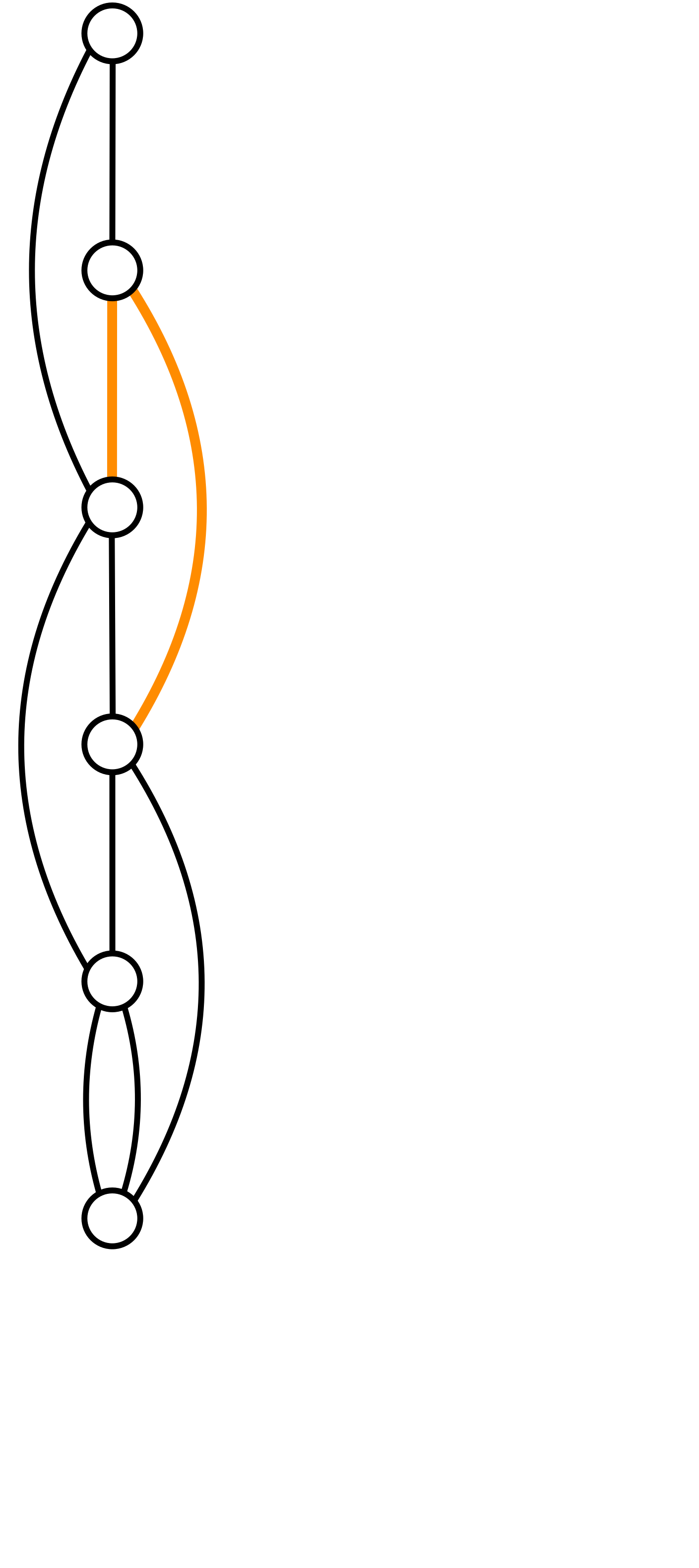
(a)

Figure 3: The construction with the level $Y_{2}$ highlighted in orange.

We use the following definition:

Definition 16.

We say that the tree-packing $\mathcal{T}$ on $G_{k,n}$ is in standard position if the following holds:

• $|\mathcal{T}|=2j$ for some $j\in\mathbb{Z}$.

• For all $i$: $Y_{i}$ is at level $\beta_{i}$ for some $\beta_{i}$.

• For all $i<j$, we have that: $\beta_{i}\geq\beta_{j}$ and that $|\beta_{i}-\beta_{i-1}|\leq 1$.

• $\beta_{2k-1}\geq 0$.

• For all $i$: $f^{i}_{2}$ has been packed $j$ times.

• There is some $\iota$ such that for all $i\geq\iota$: $f^{i}_{1}$ has been packed $j$ times, and for all $i<\iota$ $f^{i}_{1}$ has been packed $j-1$ times.

We let the vector $\beta=(\beta_{1},\beta_{2},\dots,\beta_{2k})\in\mathbb{Z}^{2k}$ be the level profile of $\mathcal{T}$.

Next we will show that if $\mathcal{T}$ is in standard position with $\text{lev}(Y_{i})=\text{lev}(Y_{i+1})$ for some $i$, then we can increase the level of some $Y_{j}$ without decreasing the level of any pair by adding only $O(k)$ trees to $\mathcal{T}$ while still ensuring that $\mathcal{T}$ ends up in standard position. The final tree-packing is then achieved by applying the above procedure in a systematic way $O(k^{2})$ times. Note that the empty packing is in standard position. Before showing this, we first show the following lemma.

Lemma 17.

Let $\mathcal{T}$ be a greedy tree-packing in standard position on $G_{n,k}$ with $|\mathcal{T}|=2j$ and $\beta_{2k}\geq 0$. Let $i$ and $s\geq 1$ be such that 1) either $\beta_{i}=\beta_{i+1}=\dots=\beta_{i+s}>\beta_{i+s+1}$ or $\beta_{i}=\beta_{i+1}=\dots=\beta_{i+s}$ and $i+s=2j$, and 2) either $\beta_{i-1}>\beta_{i}$ or $i=1$. Then there is a greedy tree-packing $\mathcal{T}^{\prime}$ in standard position on $G_{n,k}$ with $2j+2(\mathopen{}\lfloor\tfrac{s}{2}\rfloor\mathclose{}+1)$ trees such that the level profile $\beta^{\prime}$ of $\mathcal{T}^{\prime}$ satisfies $\beta^{\prime}_{l}=\beta_{l}+[i=l]-[i+s=l]$ for all $l$.

Proof.

We will show the lemma assuming that $\beta_{i}=\beta_{i+1}=\dots=\beta_{i+s}>\beta_{i+s+1}$ and that $\beta_{i-1}>\beta_{i}$. The other cases follow from analogous arguments.

We pack trees in pairs. Consider first the following trees $T$ and $T^{\prime}$ that greedily extends $\mathcal{T}$. The edge $e^{l}_{1}$ is in $T$ if $\text{lev}(Y_{l})$ is even, $e^{l}_{2}$ is in $T$ if $\text{lev}(Y_{l})$ is odd, and all edges $f^{p}_{1}$ are in $T$. In order to verify that $T$ indeed extends $\mathcal{T}$ in a greedy manner, observe that since $\mathcal{T}$ is in standard position, it follows by downward induction on $l$ that $T$ extends $\mathcal{T}$ greedily. See Figure 4 for an illustration.

Similarly, we let $e^{j}_{2}$ in $T^{\prime}$ if $\text{lev}(Y_{j})$ is even, $e^{j}_{1}$ in $T^{\prime}$ if $\text{lev}(Y_{j})$ is odd, and all edges $f^{j}_{2}$ are in $T$. Exactly as above, it follows by induction that $T^{\prime}$ greedily extends $\mathcal{T}\cup T$, and that $\mathcal{T}\cup\{T,T^{\prime}\}$ is a greedy tree-packing in standard position with the same level profile as $\mathcal{T}$.

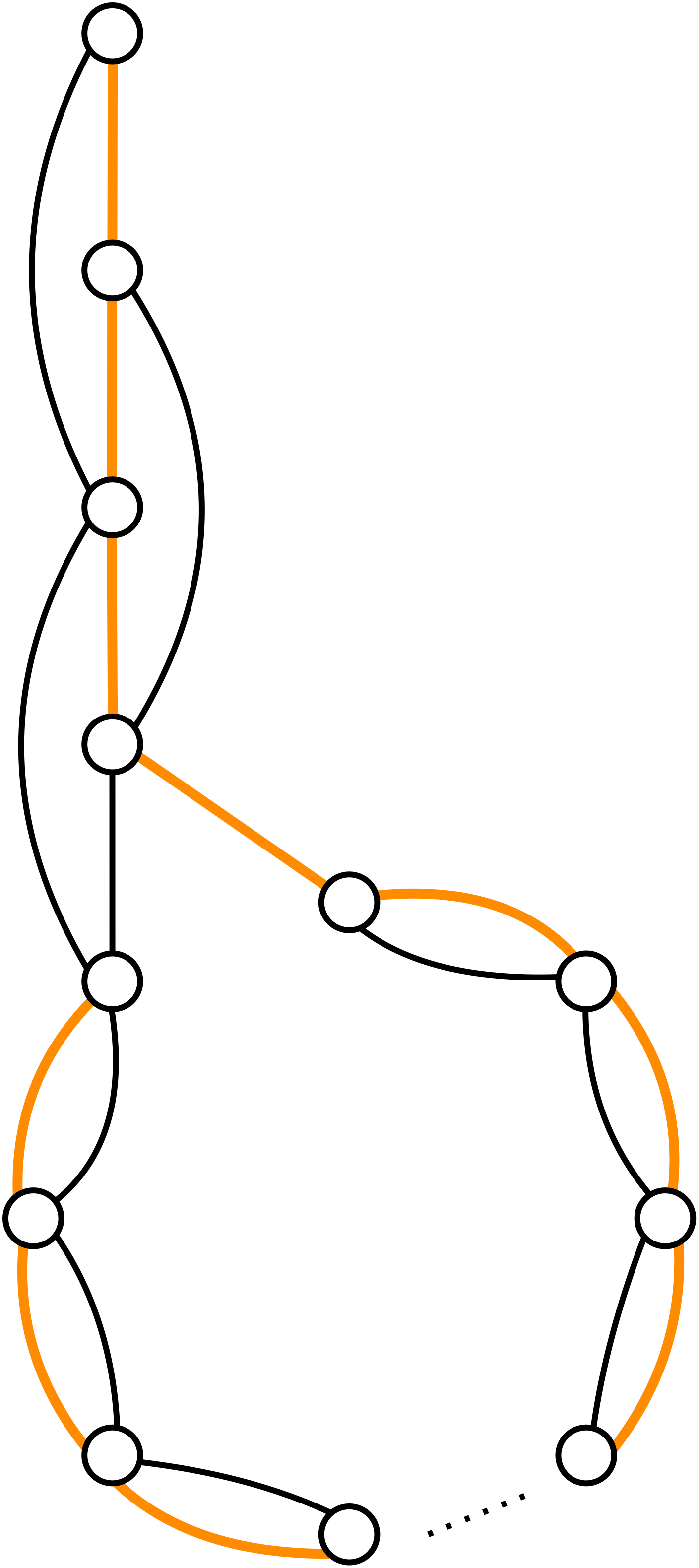
(a)

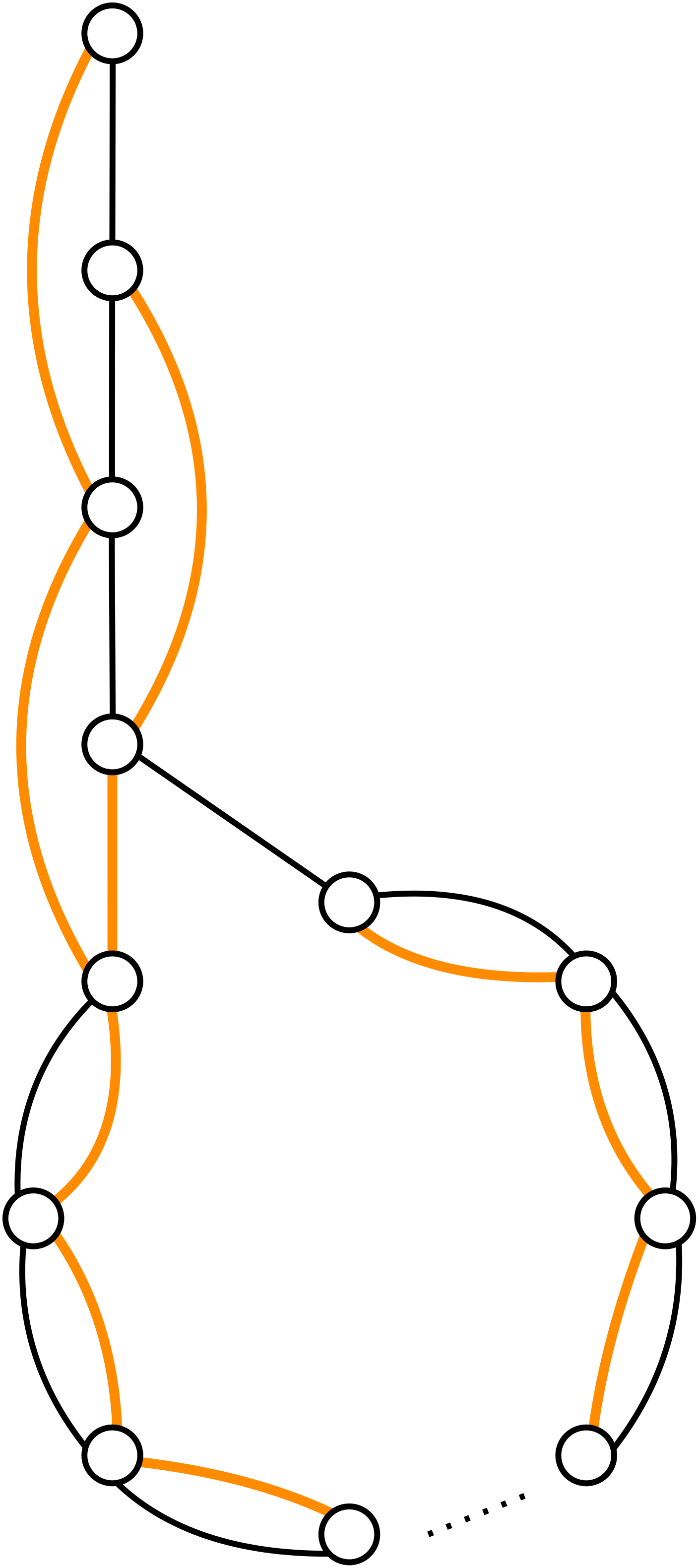
(b)

Figure 4: The figure illustrates $T$ (on the left) and $T^{\prime}$ (on the right) in the case where $i=1$, $s=3$, $\text{lev}(Y_{1})=\text{lev}(Y_{2})=\text{lev}(Y_{3})=2$, and $\text{lev}(Y_{4})=1$.

We can extend $\mathcal{T}$ as above as many times as we would like to obtain a greedy tree-packing

$$\mathcal{T}\cup\mathopen{}\left(\bigcup_{i=1}^{2(\mathopen{}\lfloor\tfrac{s}{2}\rfloor\mathclose{}+1)}\{T_{i},T^{\prime}_{i}\}\right)\mathclose{}$$

in standard position with the same level profile as $\mathcal{T}$.

Consider first the case where $\text{lev}(Y_{i})=\text{lev}(Y_{i+1})$ is even. Then, we can perform the swap of $e^{i}_{2}$ for $e^{i+1}_{1}$, while keeping $T_{1}$ a greedy extension of $\mathcal{T}$. Similarly, we can now perform the swaps $e^{i}_{1}$ for $e^{i}_{2}$ and $e^{i+1}_{1}$ for $e^{i+2}_{2}$ in $T^{\prime}_{1}$. After these swaps, $T^{\prime}_{1}$ is again a greedy extension of $\mathcal{T}\cup T_{1}$. See Figure 5 for an illustration.

(a)

(b)

Figure 5: The figure illustrates $T_{1}$ (on the left) and $T^{\prime}_{1}$ (on the right) in the case where $i=1$, $s=3$, $\text{lev}(Y_{1})=\text{lev}(Y_{2})=\text{lev}(Y_{3})=2$, and $\text{lev}(Y_{4})=1$. Observe that all edges are packed once except for $a$, which is packed twice, and $b$ which is not packed.

Next, we can change $T_{2}$ by swapping $e^{i}_{1}$ for $e^{i}_{2}$ and $e^{i+3}_{1}$ for $e^{i+2}_{2}$. Then we change $T^{\prime}_{2}$ by swapping $e^{i}_{2}$ for $e^{i}_{1}$, $e^{i+4}_{2}$ for $e^{i+3}_{1}$.

We can continue this process mutatis mutandis, until at some point we pack neither $e^{i+s}_{1}$ nor $e^{i+s}_{2}$. For even $s$, this happens in $T^{\prime}_{\tfrac{s}{2}}$, and for odd $s$, this happens in $T_{\mathopen{}\lceil\tfrac{s}{2}\rceil\mathclose{}}$. For even $s$, we make no more changes. For odd $s$, we need still need to change $T^{\prime}_{\mathopen{}\lceil\tfrac{s}{2}\rceil\mathclose{}}$: we swap $e^{i}_{2}$ for $e^{i}_{1}$ and $e^{i+s}_{2}$ for $e^{i+s}_{1}$.

It follows by induction on $s$ that

$$\mathcal{T}^{\prime}=\mathcal{T}\cup\mathopen{}\left(\bigcup_{i=1}^{2(\mathopen{}\lfloor\tfrac{s}{2}\rfloor\mathclose{}+1)}\{T_{i},T^{\prime}_{i}\}\right)\mathclose{}$$

is a greedy tree-packing in standard position with the claimed level profile. If needed, we can increase the size of the tree-packing to the required size by adding another pair of $T$ and $T^{\prime}$ (based on the levels of $\mathcal{T}^{\prime}$ and not of $\mathcal{T}$).

In the case where $\text{lev}(Y_{i})=\text{lev}(Y_{i+1})$ is odd, we only alter $T^{\prime}_{1}$. Here, we exchange $e^{i+1}_{1}$ for $e^{i}_{2}$.

Next we perform the following swaps on $T_{2}$; we swap $e^{i}_{2}$ for $e^{i}_{1}$, and we swap $e^{i+2}_{2}$ for $e^{i+1}_{1}$. We change $T^{\prime}_{2}$ by swapping $e^{i}_{1}$ for $e^{i}_{2}$ and we swap $e^{i+3}_{1}$ for $e^{i+2}_{2}$.

We can continue this process mutatis mutandis, until at some point we pack neither $e^{i+s}_{1}$ nor $e^{i+s}_{2}$. For even $s$, this happens in $T_{\tfrac{s}{2}+1}$, and for odd $s$, this happens in $T^{\prime}_{\mathopen{}\lceil\tfrac{s}{2}\rceil\mathclose{}}$. For odd $s$, we stop here. For even $s$, we need still need to pack $T^{\prime}_{\tfrac{s}{2}+1}$ before stopping. Before doing so, we swap $e^{i}_{1}$ for $e^{i}_{2}$ and $e^{i+s}_{1}$ for $e^{i+s}_{2}$.

It follows by induction on $s$ that

$$\mathcal{T}\cup\mathopen{}\left(\bigcup_{i=1}^{2(\mathopen{}\lfloor\tfrac{s}{2}\rfloor\mathclose{}+1)}\{T_{i},T^{\prime}_{i}\}\right)\mathclose{}$$

is a greedy tree-packing in standard position with the claimed level profile. ∎

We can now use this lemma to extend the packing.

Lemma 18.

Let $\mathcal{T}$ be a greedy tree-packing in standard position on $G_{n,k}$ with $|\mathcal{T}|=2j$ and $\beta_{2k}\in\{0,1\}$. Let $i$ and $s>0$ be such that 1) either $\beta_{i}=\beta_{i+1}=\dots=\beta_{i+s}>\beta_{i+s+1}$ or $\beta_{i}=\beta_{i+1}=\dots=\beta_{i+s}$ and $i+s=2j$, and 2) either $\beta_{i-1}>\beta_{i}$ or $i=1$. Then there is a greedy tree-packing $\mathcal{T}^{\prime}$ in standard position on $G_{n,k}$ with $2j+2(2k+1)$ trees such that the level profile $\beta^{\prime}$ of $\mathcal{T}^{\prime}$ satisfies $\beta^{\prime}_{l}=\beta_{l}+[i=l]$ for all $l$.

Proof.

We will show the lemma assuming that $\beta_{i}=\beta_{i+1}=\dots=\beta_{i+s}>\beta_{i+s+1}$ and that $\beta_{i-1}>\beta_{i}$. The other cases follow from identical arguments.

We begin by letting $t=i$, $s^{\prime}=s$. Then we apply Lemma 17 with $t$ and $s^{\prime}$ as arguments to get a new packing with only $2j+2(\mathopen{}\lfloor\tfrac{s^{\prime}}{2}\rfloor\mathclose{}+1)$ trees. We then let $t=t+s^{\prime}$ and $s^{\prime}$ be the smallest non-negative integer such that $\text{lev}(Y_{t})>\text{lev}(Y_{t+s^{\prime}})$. Again we apply Lemma 17 with $t$ and $s^{\prime}$ as arguments. We do this recursively, until $t+s^{\prime}=2k$.

At this point, we have a tree-packing $\mathcal{T}^{\prime}$ of size at most $2j+4k$. Indeed, in the worst-case $s^{\prime}=0$ in every iteration, leaving us with at most $2k$ recursive calls.

If the initial level of $Y_{2k}$ was $1$, we pack $T$ with $e^{2k}_{2}$ and $f^{\iota}_{1}$ swapped. Then we pack $T^{\prime}$, but with $e^{2k}_{1}$ and $e^{2k}_{2}$ swapped. Note here that $T$ and $T^{\prime}$ should be constructed with respect to the levels of $\mathcal{T}^{\prime}$ and not $\mathcal{T}$.

If the initial level of $Y_{2k}$ was $0$, we pack $T$ with $e^{2k}_{1}$ and $f^{\iota}_{1}$ swapped. Then we pack $T^{\prime}$, but with $e^{2k}_{1}$ and $e^{2k}_{2}$ swapped. Again $T$ and $T^{\prime}$ should be constructed with respect to the levels of $\mathcal{T}^{\prime}$ and not $\mathcal{T}$.

Finally, we can, if necessary, pad with un-altered copies of $T$ and $T^{\prime}$ (based on the levels of the final tree-packing above) to achieve a greedy tree-packing of the form

$$\mathcal{T}\cup\mathopen{}\left(\bigcup_{l=1}^{2(2k+1)}\{T_{l},T^{\prime}_{l}\}\right)\mathclose{}$$

in standard position with $\iota$ one larger than before. Observe that the ultimate tree-packing has level profile

$$\hat{\beta}_{l}=\beta_{l}+[l=2k]+\sum_{(t,s^{\prime})}[l=t]-[l=t+s^{\prime}]=\beta_{l}+[l=i]+\sum_{t}-[l=t]+[l=t]=\beta_{l}+[l=i],$$

as claimed. ∎

To obtain the final tree-packing of $G_{n,k}$ we do as follows. Beginning from the empty packing, which is in standard position, we repeatedly apply Lemma 18. The goal is to achieve a level profile of the form $(2k-1,2k-2,\dots,0)$. To do so, assume that we have constructed a level profile of the form $(i,i,\dots,i,i-1,i-2,\dots,0)$. We then apply Lemma 18 on $j$ beginning with $j=1$, then $j=2$ and so on up to and including $j=2k-i$ to increase the $j^{th}$ coordinate to $i+1$.

Since we apply Lemma 18 $\sum\limits_{j=1}^{2k}j=k(2k+1)$ times, and each application extends the tree-packing with $2(2k+1)$ trees, the resulting tree-packing $\mathcal{T}$ contains $2k(2k+1)^{2}$ trees. Since the tree-packing is in standard position, we observe that some edge $e$ has been packed $\tfrac{|\mathcal{T}|}{2}+k$ times. By Lemma 15 we have that $\ell^{*}(e)=\tfrac{1}{2}$, so if

$$\frac{k}{|\mathcal{T}|}=\frac{k}{2k(2k+1)^{2}}=|\ell^{\mathcal{T}}(e)-\ell^{*}(e)|\leq\frac{\varepsilon}{2}$$

we have that

$$\varepsilon^{-1}\leq(2k+1)^{2}$$

i.e., $k=\Omega(\varepsilon^{-\tfrac{1}{2}})$. In particular, the lemma now follows for $\lambda=2$. Indeed, the above construction with specific $k=O(\varepsilon^{-\tfrac{1}{2}})$ yields a tree-packing with $\Omega(\lambda\cdot{}\varepsilon^{-3/2})$ trees that does not achieve the required concentration. Note that this only holds for large enough $\varepsilon$ with $\varepsilon^{-1}\in O(n^{1/3})$, since otherwise $\iota$ might become too big for the argument in Lemma 18 to go through.

To generalize the statement to any $\lambda\in 2\mathbb{Z}$, let $\lambda=2s$. Then we get $G_{s,n,k}$ by duplicating every edge of $G_{n,k}$ $s$ times. We get a greedy tree-packing $\mathcal{T}_{s}$ by replacing each tree $T$ in the tree-packing $\mathcal{T}$ on $G_{n,k}$ by $s$ parallel and isomorphic copies of $T$, each using their own set of edges.

In total $|\mathcal{T}_{s}|=2k(2k+1)^{2}\cdot{}s$, and so the calculation now becomes:

$$\frac{k}{|\mathcal{T}|}=\frac{k}{2k(2k+1)^{2}\cdot{}s}=|\ell^{\mathcal{T}}(e)-\ell^{*}(e)|\leq\frac{\varepsilon}{2s}$$

and again we conclude that

$$\varepsilon^{-1}\leq(2k+1)^{2}$$

and obtain the theorem exactly as before.

5 Existence of Small Tree-Packing

The goal of this section is to show that for all graphs $G$ there exists a tree-packing that approximates the ideal load decomposition well. Formally, we will prove the following.

* We restate the theorem slightly. We recall that $\lambda/2<\Phi\leq\lambda$ by Lemma 2. Hence the statement is equivalent to $|\mathcal{T}|=\Theta(\Phi/\varepsilon)$ trees guaranteeing

$$|\ell^{\mathcal{T}}(e)-\ell^{*}(e)|\leq\varepsilon/\Phi,$$

for all $e\in E$.

To show this, we first inspect the easier case, where the trivial partition $\mathcal{P}=\{v_{i}\}_{i=1}^{n}$ achieves the minimum partition value $\Phi_{G}$ of $G$.

To do so, we will generalize Kaiser’s simple proof of the tree-packing theorem [Kai12], to packing trees plus one forest. The proof is very similar to the proof in [Kai12], we include it for completeness. We start by introducing some notation.

Let $k\geq 1$. A $k$-decomposition $\mathcal{T}$ of a graph is a $k$-tuple of spanning subgraphs such that $\{E(T_{i}):1\leq i\leq k\}$ is a partition of $E(G)$.

We define the sequence $(\mathcal{P}_{0},\mathcal{P}_{1},\dots,\mathcal{P}_{\infty})$ of partitions of $V(G)$ associated with $\mathcal{T}$ as follows. First $\mathcal{P}_{0}=\{V(G)\}$. For $i\geq 0$, if there exists $c\in\{1,\dots,k\}$ such that the induced subgraph $T_{c}[X]$ is disconnected for some $X\in\mathcal{P}_{i}$, then let $c_{i}$ be the least such $c$, and let $\mathcal{P}_{i+1}$ consist of the vertex sets of all components of $T_{c_{i}}[X]$, where $X$ ranges over all the classes of $\mathcal{P}_{i}$. Otherwise, the process ends by setting $\mathcal{P}_{\infty}=\mathcal{P}_{i}$, and we set $c_{j}=k+1$ and $\mathcal{P}_{j}=\mathcal{P}_{i}$ for all $j\geq i$.

The level, $\operatorname{level}(e)$, of an edge $e\in E(G)$ (w.r.t. $\mathcal{T}$) is defined as the largest $i$ (possibly $\infty$) such that both endpoints of $e$ are contained in one class in $\mathcal{P}_{i}$.

When $\mathcal{P}$ and $\mathcal{Q}$ are partitions of $V(G)$, we say that $\mathcal{P}$ refines $\mathcal{Q}$, denoted by $\mathcal{P}\leq Q$, if every class of $\mathcal{P}$ is a subset of a class of $\mathcal{Q}$.

Finally, we define a strict partial order on $k$-decompositions. Given two $k$-decompositions $\mathcal{T}$ and $\mathcal{T}^{\prime}$, we set $\mathcal{T}\prec\mathcal{T}^{\prime}$ if there is some finite $j\geq 0$ such that both of the following hold

• for $0\leq i<j$, $\mathcal{P}_{i}=\mathcal{P}_{i}^{\prime}$ and $c_{i}=c_{i}^{\prime}$,

• either $\mathcal{P}_{j}<\mathcal{P}_{j}^{\prime}$ or $\mathcal{P}_{j}=\mathcal{P}_{j}^{\prime}$ and $c_{j}<c_{j}^{\prime}$.

Lemma 19.

Let $G$ be a graph on vertex set $V(G)=\{v_{1},v_{2},\dots,v_{n}\}$ such that the trivial partition $\mathcal{P}=\{v_{i}\}_{i=1}^{n}$ achieves the minimum partition value $\Phi_{G}$ of $G$. Then, there exists a disjoint packing with $\lfloor\Phi_{G}\rfloor$ spanning trees and one forest $F$ on exactly $(\Phi_{G}-\lfloor\Phi_{G}\rfloor)(n-1)$ edges.

Proof.

The idea is the following: pick a $k$-decomposition that first of all contains $\lfloor\Phi_{G}\rfloor$ disjoint spanning trees and (at most) one disjoint spanning subgraph $F$ on $(\Phi_{G}-\lfloor\Phi_{G}\rfloor)(n-1)$ edges, that subject to these constraints maximize the partial order $\prec$. Note that this is a $k$-decomposition for $k=\mathopen{}\lceil\Phi_{G}\rceil\mathclose{}$, and that there is only a forest $F$ iff $\Phi_{G}$ is non-integer. If $\Phi_{G}$ is integer the statement is exactly the tree-packing theorem, so follows by e.g. [Kai12]. So we assume it is not. In that case $F=T_{k}$.

The claim now is that $\mathcal{P}=\mathcal{P}_{\infty}$ has at least $(\Phi_{G}-\lfloor\Phi_{G}\rfloor)(n-1)$ non-parallel, inter-partition edges. If $F$ is a forest, we are done.

We first argue that if $F$ is not a forest, then $F$ must contain a cycle in $G/\mathcal{P}$. To see this, consider $G/\mathcal{P}$. Since $T_{i}$ and $F$ all induce trees inside each partition of $\mathcal{P}$, we conclude that $F$ must have at least $(\Phi_{G}-\lfloor\Phi_{G}\rfloor)(|\mathcal{P}|-1)$ edges in $G/\mathcal{P}$. $F$ contains a tree on each partition $P\in\mathcal{P}$ so we have at least $n-|\mathcal{P}|$ edges inside the partitions. Now we see that

$$(\Phi_{G}-\lfloor\Phi_{G}\rfloor)(n-1)=|E(F)|\geq(\Phi_{G}-\lfloor\Phi_{G}\rfloor)(|\mathcal{P}|-1)+(n-|\mathcal{P}|).$$

Rearranging gives

$$(\Phi_{G}-\lfloor\Phi_{G}\rfloor)(n-|\mathcal{P}|)\geq n-|\mathcal{P}|,$$

and thus for $|\mathcal{P}|\neq n$, $\Phi_{G}-\lfloor\Phi_{G}\rfloor\geq 1$, a contradiction. We conclude that $|\mathcal{P}|=n$, and thus any cycle in $F$ is a cycle in $F/\mathcal{P}$.

Let $e$ be an edge in a cycle of $F=T_{k}$ of minimum level, and set $m=\operatorname{level}(e)$. Let $P$ be the class of of $\mathcal{P}_{m}$ containing both endpoints of $e$. Since $e$ joins different components of $T_{c_{m}}[P]$, we have $c_{m}\neq k$, and the unique cycle $C$ in $T_{c_{m}}+e$ contains an edge with only one endpoint in $P$. Thus for some edge $e^{\prime}\in C$ we have $\operatorname{level}(e^{\prime})<m$. Let $e^{\prime}$ be such an edge of lowest level. Let $Q$ be the class of $\mathcal{P}_{\operatorname{level}(e^{\prime})}$ containing both endpoints of $e^{\prime}$. Observe that $V(C)\subseteq Q$. We now create a new $k$-decomposition with $e$ and $e^{\prime}$ swapped: let $\mathcal{T}^{\prime}$ be the $k$-decomposition obtained from $\mathcal{T}$ by replacing $T_{c_{m}}$ with $T_{c_{m}}+e-e^{\prime}$ and $T_{k}$ with $T_{k}-e+e^{\prime}$.

Next, it is easy to check that $\mathcal{T}\prec\mathcal{T}^{\prime}$, contradicting that $\mathcal{T}$ was maximal. First, we show that for $i\leq m$ we have $\mathcal{P}_{i}^{\prime}=\mathcal{P}_{i}$ and $c_{i}^{\prime}=c_{i}$. We do this by induction. For $i=0$ we have $\mathcal{P}_{0}^{\prime}=\{V(G)\}=\mathcal{P}_{0}$ and $c_{0}^{\prime}=k=c_{0}$, so the base case is clear. Now we assume that the statement holds for $0\leq i<m$, and we prove it for $i+1$.

Let $S$ be an arbitrary class of $\mathcal{P}_{i+1}$, by definition, $T_{c_{i}}[S]$ is connected. We want to show that $T^{\prime}_{c_{i}^{\prime}}[S]$ is also connected. By the induction hypothesis, $c_{i}^{\prime}=c_{i}$. If $c_{i}\notin\{c_{m},k\}$, then $T^{\prime}_{c_{i}^{\prime}}[S]=T_{c_{i}^{\prime}}[S]=T_{c_{i}}[S]$, so is connected. We have $i<m$, so we are only left with the case $c_{i}=k$. We have that $E(T_{k})-E(T_{k}^{\prime})=e$, so if not both endpoints of $e$ are in $S$, then we have $T_{k}^{\prime}[S]$ is connected as well. If $S$ does contain both endpoints of $e$, then $P\subseteq S$, because every class of $\mathcal{P}_{i+1}$ containing both endpoints of $e$ contains $P$. Hence $T_{k}^{\prime}[S]$ is connected. We see that $\mathcal{P}_{i+1}\leq\mathcal{P}_{i+1}^{\prime}$. By maximality of $\mathcal{T}$, we conclude that $\mathcal{P}_{i+1}=\mathcal{P}_{i+1}^{\prime}$.

Next, we show that $c_{i+1}^{\prime}=c_{i+1}$. Let $R\in\mathcal{P}_{i+1}$ and $c<c_{i+1}$. Since $\mathcal{P}_{i+1}=\mathcal{P}_{i+1}^{\prime}$, we have $R\in\mathcal{P}_{i+1}^{\prime}$. By definition of $c_{i+1}$, $T_{c}[R]$ is connected. Similar as before, we can argue that $T_{c}^{\prime}[R]$ is connected. Hence, $c_{i+1}^{\prime}\geq c_{i+1}$. Again by maximality of $\mathcal{T}$, we get that we must have $c_{i+1}^{\prime}=c_{i+1}$.

Now we look at the next step. We have from the above that $\mathcal{P}_{m}^{\prime}=\mathcal{P}_{m}$ and $c_{m}^{\prime}=c_{m}$, so the classes of $\mathcal{P}_{m+1}^{\prime}$ are the vertex set of components of $T_{c_{m}}^{\prime}[U]$ for $U\in\mathcal{P}_{m}$. For $U\in\mathcal{P}_{m}-\{P\}$, we have $T_{c_{m}}^{\prime}[U]=T_{c_{m}}[U]$, so their components coincide. The graph $T_{c_{m}}^{\prime}[P]$ equals $T_{c_{m}}[P]$ with the extra edge $e$ connecting two components of $T_{c_{m}}[P]$. Hence $\mathcal{P}_{m+1}<\mathcal{P}_{m+1}^{\prime}$, so also $\mathcal{T}\prec\mathcal{T}^{\prime}$, contradicting $\mathcal{T}$ being maximal. ∎

Now the result follows easily on graphs with uniform $\Phi_{G}$.

Lemma 20.

Let $G$ be an unweighted, undirected (multi-) graph, where the trivial partition $\mathcal{P}=\{v_{i}\}_{i=1}^{n}$ achieves the minimum partition value $\Phi_{G}$ of $G$. There exists a tree-packing $\mathcal{T}$ that needs $|\mathcal{T}|=\Theta(\Phi_{G}/\varepsilon)$ trees to satisfy

$$|\ell^{\mathcal{T}}(e)-\ell^{*}(e)|\leq\varepsilon/\Phi_{G},$$

for all $e\in E$.

Proof.

W.l.o.g., assume that $1/\varepsilon$ is an integer. We replace every edge in $G$ by $1/\varepsilon$ copies to obtain $G^{\prime}$. Note that $\ell^{*}_{G^{\prime}}(e)=\varepsilon\ell^{*}_{G}(e)$ and $\Phi_{G^{\prime}}=\Phi_{G}/\varepsilon$. By Lemma 19, we see that we can pack $\lfloor\Phi_{G^{\prime}}\rfloor$ spanning trees and one forest on exactly $(\Phi_{G^{\prime}}-\lfloor\Phi_{G^{\prime}}\rfloor)(n-1)$ edges. Now let $\mathcal{T}$ consists of these $\lfloor\Phi_{G^{\prime}}\rfloor$ spanning trees, together with one tree that is the forest extended to a tree in an arbitrary way. Now we have that $L^{\mathcal{T}}(e)=1/\varepsilon$ or $L^{T}(e)=1/\varepsilon+1$. We see that in the first case that

$$|\ell^{\mathcal{T}}(e)-\ell^{*}(e)| =\left|\frac{1/\varepsilon}{\lceil\Phi_{G}/\varepsilon\rceil}-\frac{1}{\Phi_{G}}\right|=\frac{1}{\Phi_{G}}-\frac{1/\varepsilon}{\lceil\Phi_{G}/\varepsilon\rceil}=\frac{\lceil\Phi_{G}/\varepsilon\rceil-\Phi_{G}/\varepsilon}{\lceil\Phi_{G}/\varepsilon\rceil\Phi_{G}}$$

$$\leq\frac{1}{\lceil\Phi_{G}/\varepsilon\rceil\Phi_{G}}\leq\varepsilon/\Phi_{G}.$$

And in the second case we have

$$|\ell^{\mathcal{T}}(e)-\ell^{*}(e)| =\left|\frac{1/\varepsilon+1}{\lceil\Phi_{G}/\varepsilon\rceil}-\frac{1}{\Phi_{G}}\right|=\left|\frac{\Phi_{G}/\varepsilon+\Phi_{G}-\lceil\Phi_{G}/\varepsilon\rceil}{\lceil\Phi_{G}/\varepsilon\rceil\Phi_{G}}\right|$$

$$\leq\left|\frac{\Phi_{G}/\varepsilon-\lceil\Phi_{G}/\varepsilon\rceil}{\lceil\Phi_{G}/\varepsilon\rceil\Phi_{G}}\right|+\left|\frac{\Phi_{G}}{\lceil\Phi_{G}/\varepsilon\rceil\Phi_{G}}\right|\leq 2\varepsilon/\Phi_{G},$$

where for the first inequality we use the triangle inequality, and for the second inequality we use the first case. Now by setting $\varepsilon\leftarrow\varepsilon/2$, we obtain the result. ∎

At last, we are ready to show the general case.

Proof of Section 1.3.

We recall the definition of the ideal relative loads: $\ell^{*}(e)$ is defined recursively as follows.

1. Let $\mathcal{P}^{*}$ be a packing with $\rm{pack\_val}(\mathcal{P}^{*})=\Phi$.

2. For all $e\in E(G/\mathcal{P})$, set $\ell^{*}(e):=1/\Phi$.

3. For each $S\in\mathcal{P}^{*}$, recurse on the subgraph $G[S]$.

We prove the lemma by induction on the depth of this recursive definition. If the depth is $0$ then the minimum partition value $\Phi_{G}$ is exactly achieved by the trivial partition $\mathcal{P}=\{v_{i}\}_{i=1}^{n}$, so the base case is immediate. Suppose it holds up to depth $i$. Then we have for each component $X\in\mathcal{P}^{*}$ that there exists a tree-packing $\mathcal{T}_{X}$ such that $|\mathcal{T}_{X}|=\Theta(\Phi/\varepsilon)$ and

$$|\ell^{\mathcal{T}_{X}}(e)-\ell^{*}(e)|\leq\varepsilon/\Phi,$$

for all $e\in E(G[X])$. Note that this follows from the induction hypothesis since $\Phi_{G[X]}\geq\Phi$, so we can set $\varepsilon\leftarrow\tfrac{\Phi_{G[X]}}{\Phi}\varepsilon$. We also have a tree-packing $\mathcal{T}_{\mathcal{P}*}$ on $G/\mathcal{P}^{*}$ such that $|\mathcal{T}_{\mathcal{P}^{*}}|=\Theta(\Phi/\varepsilon)$ and

$$|\ell^{\mathcal{T}_{\mathcal{P}^{*}}}(e)-\ell^{*}(e)|\leq\varepsilon/\Phi,$$

for all $e\in E(G/\mathcal{P}^{*})$. Clearly $\mathcal{T}=\mathcal{T}_{\mathcal{P}^{*}}\cup\left(\bigcup_{X\in\mathcal{P}^{*}}\mathcal{T}_{X}\right)$, where each tree is a union of the respective trees, is a tree-packing of $G$ that satisfies the bounds on $\ell^{\mathcal{T}}$. ∎

References

- [AHK12] Sanjeev Arora, Elad Hazan and Satyen Kale “The Multiplicative Weights Update Method: a Meta-Algorithm and Applications” In Theory Comput. 8.1, 2012, pp. 121–164 DOI: 10.4086/TOC.2012.V008A006
- [AHLT05] Stephen Alstrup, Jacob Holm, Kristian Lichtenberg and Mikkel Thorup “Maintaining information in fully dynamic trees with top trees” In ACM Trans. Algorithms 1.2, 2005, pp. 243–264 DOI: 10.1145/1103963.1103966
- [BF20] Markus Blumenstock and Frank Fischer “A Constructive Arboricity Approximation Scheme” In SOFSEM 2020: Theory and Practice of Computer Science - 46th International Conference on Current Trends in Theory and Practice of Informatics, SOFSEM 2020, Limassol, Cyprus, January 20-24, 2020, Proceedings 12011, Lecture Notes in Computer Science Springer, 2020, pp. 51–63 DOI: 10.1007/978-3-030-38919-2\_5
- [BF99] Gerth Stølting Brodal and Rolf Fagerberg “Dynamic Representation of Sparse Graphs” In Algorithms and Data Structures, 6th International Workshop, WADS ’99, Vancouver, British Columbia, Canada, August 11-14, 1999, Proceedings 1663, Lecture Notes in Computer Science Springer, 1999, pp. 342–351 DOI: 10.1007/3-540-48447-7\_34
- [BHNT15] Sayan Bhattacharya, Monika Henzinger, Danupon Nanongkai and Charalampos E. Tsourakakis “Space- and Time-Efficient Algorithm for Maintaining Dense Subgraphs on One-Pass Dynamic Streams” In Proceedings of the Forty-Seventh Annual ACM on Symposium on Theory of Computing, STOC 2015, Portland, OR, USA, June 14-17, 2015 ACM, 2015, pp. 173–182 DOI: 10.1145/2746539.2746592
- [BP12] Karl Bringmann and Konstantinos Panagiotou “Efficient Sampling Methods for Discrete Distributions” In Automata, Languages, and Programming - 39th International Colloquium, ICALP 2012, Warwick, UK, July 9-13, 2012, Proceedings, Part I 7391, Lecture Notes in Computer Science Springer, 2012, pp. 133–144 DOI: 10.1007/978-3-642-31594-7\_12
- [BRS20] Niranka Banerjee, Venkatesh Raman and Saket Saurabh “Fully dynamic arboricity maintenance” Announced at COCOON 2019 In Theor. Comput. Sci. 822, 2020, pp. 1–14 DOI: 10.1016/J.TCS.2020.04.010
- [BS15] Aaron Bernstein and Cliff Stein “Fully Dynamic Matching in Bipartite Graphs” In Automata, Languages, and Programming - 42nd International Colloquium, ICALP 2015, Kyoto, Japan, July 6-10, 2015, Proceedings, Part I, 2015, pp. 167–179
- [BS16] Aaron Bernstein and Cliff Stein “Faster Fully Dynamic Matchings with Small Approximation Ratios” In Proceedings of the Twenty-Seventh Annual ACM-SIAM Symposium on Discrete Algorithms, SODA 2016, Arlington, VA, USA, January 10-12, 2016, 2016, pp. 692–711
- [CCHH+24] Chandra Chekuri et al. “Adaptive Out-Orientations with Applications” In Proceedings of the 2024 Annual ACM-SIAM Symposium on Discrete Algorithms (SODA), 2024, pp. 3062–3088 SIAM arXiv:2310.18146
- [CGLN+20] Julia Chuzhoy et al. “A Deterministic Algorithm for Balanced Cut with Applications to Dynamic Connectivity, Flows, and Beyond” In 61st IEEE Annual Symposium on Foundations of Computer Science, FOCS 2020, Durham, NC, USA, November 16-19, 2020 IEEE, 2020, pp. 1158–1167 DOI: 10.1109/FOCS46700.2020.00111
- [CQX19] Chandra Chekuri, Kent Quanrud and Chao Xu “LP Relaxation and Tree Packing for Minimum k-cuts” In 2nd Symposium on Simplicity in Algorithms, SOSA 2019, January 8-9, 2019, San Diego, CA, USA 69, OASIcs Schloss Dagstuhl - Leibniz-Zentrum für Informatik, 2019, pp. 7:1–7:18 DOI: 10.4230/OASICS.SOSA.2019.7
- [CQX20] Chandra Chekuri, Kent Quanrud and Chao Xu “LP Relaxation and Tree Packing for Minimum k-Cut” Announced at SOSA 2019 In SIAM J. Discret. Math. 34.2, 2020, pp. 1334–1353 DOI: 10.1137/19M1299359
- [DEMN21] Michal Dory, Yuval Efron, Sagnik Mukhopadhyay and Danupon Nanongkai “Distributed weighted min-cut in nearly-optimal time” In STOC ’21: 53rd Annual ACM SIGACT Symposium on Theory of Computing, Virtual Event, Italy, June 21-25, 2021 ACM, 2021, pp. 1144–1153 DOI: 10.1145/3406325.3451020
- [DHNS19] Mohit Daga, Monika Henzinger, Danupon Nanongkai and Thatchaphol Saranurak “Distributed edge connectivity in sublinear time” In Proceedings of the 51st Annual ACM SIGACT Symposium on Theory of Computing, STOC 2019, Phoenix, AZ, USA, June 23-26, 2019 ACM, 2019, pp. 343–354 DOI: 10.1145/3313276.3316346
- [EGIN97] David Eppstein, Zvi Galil, Giuseppe F. Italiano and Amnon Nissenzweig “Sparsification - a technique for speeding up dynamic graph algorithms” Announced at FOCS 1992 In J. ACM 44.5, 1997, pp. 669–696 DOI: 10.1145/265910.265914
- [ELS15] Alessandro Epasto, Silvio Lattanzi and Mauro Sozio “Efficient Densest Subgraph Computation in Evolving Graphs” In Proceedings of the 24th International Conference on World Wide Web, WWW 2015, Florence, Italy, May 18-22, 2015 ACM, 2015, pp. 300–310 DOI: 10.1145/2736277.2741638
- [Epp94] David Eppstein “Arboricity and Bipartite Subgraph Listing Algorithms” In Inf. Process. Lett. 51.4, 1994, pp. 207–211 DOI: 10.1016/0020-0190(94)90121-X
- [Fre85] Greg N. Frederickson “Data Structures for On-Line Updating of Minimum Spanning Trees, with Applications” Announced at STOC 1983 In SIAM J. Comput. 14.4, 1985, pp. 781–798 DOI: 10.1137/0214055
- [Fre97] Greg N. Frederickson “Ambivalent Data Structures for Dynamic 2-Edge-Connectivity and k Smallest Spanning Trees” Announced at 1991 In SIAM J. Comput. 26.2, 1997, pp. 484–538 DOI: 10.1137/S0097539792226825
- [Gab95] HN Gabow “A Matroid Approach to Finding Edge Connectivity and Packing Arborescences” Announced at STOC 1991 In Journal of Computer and System Sciences 2.50, 1995, pp. 259–273
- [Gab98] Harold N. Gabow “Algorithms for Graphic Polymatroids and Parametris s-Sets” Announced at SODA 1995 In J. Algorithms 26.1, 1998, pp. 48–86 DOI: 10.1006/JAGM.1997.0904
- [GHNS+23] Gramoz Goranci et al. “Fully Dynamic Exact Edge Connectivity in Sublinear Time” In Proceedings of the 2023 ACM-SIAM Symposium on Discrete Algorithms, SODA 2023, Florence, Italy, January 22-25, 2023 SIAM, 2023, pp. 70–86 DOI: 10.1137/1.9781611977554.CH3
- [GHT18] Gramoz Goranci, Monika Henzinger and Mikkel Thorup “Incremental Exact Min-Cut in Polylogarithmic Amortized Update Time” Announced at ESA 2016 In ACM Trans. Algorithms 14.2, 2018, pp. 17:1–17:21 DOI: 10.1145/3174803
- [GI91] Zvi Galil and Giuseppe F. Italiano “Fully Dynamic Algorithms for Edge-Connectivity Problems (Extended Abstract)” In Proceedings of the 23rd Annual ACM Symposium on Theory of Computing, May 5-8, 1991, New Orleans, Louisiana, USA ACM, 1991, pp. 317–327 DOI: 10.1145/103418.103454
- [Hen97] Monika Rauch Henzinger “A Static 2-Approximation Algorithm for Vertex Connectivity and Incremental Approximation Algorithms for Edge and Vertex Connectivity” In J. Algorithms 24.1, 1997, pp. 194–220 DOI: 10.1006/JAGM.1997.0855
- [HK97] Monika Rauch Henzinger and Valerie King “Fully dynamic 2-edge connectivity algorithm in polylogarithmic time per operation” In SRC Technical Note 4, 1997
- [HK99] Monika Rauch Henzinger and Valerie King “Randomized Fully Dynamic Graph Algorithms with Polylogarithmic Time per Operation” Announced at STOC 1995 In J. ACM 46.4, 1999, pp. 502–516 DOI: 10.1145/320211.320215
- [HLT01] Jacob Holm, Kristian Lichtenberg and Mikkel Thorup “Poly-logarithmic deterministic fully-dynamic algorithms for connectivity, minimum spanning tree, 2-edge, and biconnectivity” Announced at STOC ’98 In J. ACM 48.4, 2001, pp. 723–760 DOI: 10.1145/502090.502095
- [HQC22] Elfarouk Harb, Kent Quanrud and Chandra Chekuri “Faster and Scalable Algorithms for Densest Subgraph and Decomposition” In Advances in Neural Information Processing Systems 35: Annual Conference on Neural Information Processing Systems 2022, NeurIPS 2022, New Orleans, LA, USA, November 28 - December 9, 2022, 2022 URL: http://papers.nips.cc/paper\_files/paper/2022/hash/ac8fbba029dadca99d6b8c3f913d3ed6-Abstract-Conference.html
- [HRT18] Jacob Holm, Eva Rotenberg and Mikkel Thorup “Dynamic Bridge-Finding in Õ(log n) Amortized Time” In Proceedings of the Twenty-Ninth Annual ACM-SIAM Symposium on Discrete Algorithms, SODA 2018, New Orleans, LA, USA, January 7-10, 2018 SIAM, 2018, pp. 35–52 DOI: 10.1137/1.9781611975031.3
- [JS21] Wenyu Jin and Xiaorui Sun “Fully Dynamic s-t Edge Connectivity in Subpolynomial Time (Extended Abstract)” In 62nd IEEE Annual Symposium on Foundations of Computer Science, FOCS 2021, Denver, CO, USA, February 7-10, 2022 IEEE, 2021, pp. 861–872 DOI: 10.1109/FOCS52979.2021.00088
- [JST24] Wenyu Jin, Xiaorui Sun and Mikkel Thorup “Fully Dynamic Min-Cut of Superconstant Size in Subpolynomial Time” In Proceedings of the 2024 Annual ACM-SIAM Symposium on Discrete Algorithms (SODA), 2024, pp. 2999–3026 SIAM arXiv:2401.09700
- [Kai12] Tomás Kaiser “A short proof of the tree-packing theorem” In Discret. Math. 312.10, 2012, pp. 1689–1691 DOI: 10.1016/J.DISC.2012.01.020
- [Kar00] David R Karger “Minimum cuts in near-linear time” Announced at STOC 1996 In Journal of the ACM (JACM) 47.1 ACM New York, NY, USA, 2000, pp. 46–76 arXiv:cs.DS/9812007
- [KKM13] Bruce M. Kapron, Valerie King and Ben Mountjoy “Dynamic graph connectivity in polylogarithmic worst case time” In Proceedings of the Twenty-Fourth Annual ACM-SIAM Symposium on Discrete Algorithms, SODA 2013, New Orleans, Louisiana, USA, January 6-8, 2013 SIAM, 2013, pp. 1131–1142 DOI: 10.1137/1.9781611973105.81
- [KKPS14] Tsvi Kopelowitz, Robert Krauthgamer, Ely Porat and Shay Solomon “Orienting Fully Dynamic Graphs with Worst-Case Time Bounds” In Automata, Languages, and Programming - 41st International Colloquium, ICALP 2014, Copenhagen, Denmark, July 8-11, 2014, Proceedings, Part II 8573, Lecture Notes in Computer Science Springer, 2014, pp. 532–543 DOI: 10.1007/978-3-662-43951-7\_45
- [KKPT16] Casper Kejlberg-Rasmussen, Tsvi Kopelowitz, Seth Pettie and Mikkel Thorup “Faster Worst Case Deterministic Dynamic Connectivity” In 24th Annual European Symposium on Algorithms, ESA 2016, August 22-24, 2016, Aarhus, Denmark 57, LIPIcs Schloss Dagstuhl - Leibniz-Zentrum für Informatik, 2016, pp. 53:1–53:15 DOI: 10.4230/LIPICS.ESA.2016.53
- [KT19] Ken-ichi Kawarabayashi and Mikkel Thorup “Deterministic Edge Connectivity in Near-Linear Time” In J. ACM 66.1, 2019, pp. 4:1–4:50 DOI: 10.1145/3274663
- [KY15] Philip N. Klein and Neal E. Young “On the Number of Iterations for Dantzig-Wolfe Optimization and Packing-Covering Approximation Algorithms” Announced at IPCO 1999 In SIAM J. Comput. 44.4, 2015, pp. 1154–1172 DOI: 10.1137/12087222X
- [LS11] Jakub Lacki and Piotr Sankowski “Min-Cuts and Shortest Cycles in Planar Graphs in O(n loglogn) Time” In Algorithms - ESA 2011 - 19th Annual European Symposium, Saarbrücken, Germany, September 5-9, 2011. Proceedings 6942, Lecture Notes in Computer Science Springer, 2011, pp. 155–166 DOI: 10.1007/978-3-642-23719-5\_14
- [MTVV15] Andrew McGregor, David Tench, Sofya Vorotnikova and Hoa T. Vu “Densest Subgraph in Dynamic Graph Streams” In Mathematical Foundations of Computer Science 2015 - 40th International Symposium, MFCS 2015, Milan, Italy, August 24-28, 2015, Proceedings, Part II 9235, Lecture Notes in Computer Science Springer, 2015, pp. 472–482 DOI: 10.1007/978-3-662-48054-0\_39
- [NI92] Hiroshi Nagamochi and Toshihide Ibaraki “A Linear-Time Algorithm for Finding a Sparse k-Connected Spanning Subgraph of a k-Connected Graph” In Algorithmica 7.5&6, 1992, pp. 583–596 DOI: 10.1007/BF01758778
- [NR01] Joseph Naor and Yuval Rabani “Tree packing and approximating k-cuts” In Proceedings of the Twelfth Annual Symposium on Discrete Algorithms, January 7-9, 2001, Washington, DC, USA ACM/SIAM, 2001, pp. 26–27 URL: http://dl.acm.org/citation.cfm?id=365411.365415
- [NS16] Ofer Neiman and Shay Solomon “Simple Deterministic Algorithms for Fully Dynamic Maximal Matching” In ACM Trans. Algorithms 12.1, 2016, pp. 7:1–7:15
- [NSW17] Danupon Nanongkai, Thatchaphol Saranurak and Christian Wulff-Nilsen “Dynamic Minimum Spanning Forest with Subpolynomial Worst-Case Update Time” In 58th IEEE Annual Symposium on Foundations of Computer Science, FOCS 2017, Berkeley, CA, USA, October 15-17, 2017 IEEE Computer Society, 2017, pp. 950–961 DOI: 10.1109/FOCS.2017.92
- [NW61] C St JA Nash-Williams “Edge-disjoint spanning trees of finite graphs” In Journal of the London Mathematical Society 1.1 Oxford University Press, 1961, pp. 445–450
- [NW64] C. St.J. A. Nash-Williams “Decomposition of Finite Graphs Into Forests” In Journal of the London Mathematical Society s1-39.1, 1964, pp. 12–12 DOI: https://doi.org/10.1112/jlms/s1-39.1.12
- [PS16] David Peleg and Shay Solomon “Dynamic (1 + )-Approximate Matchings: A Density-Sensitive Approach” In Proceedings of the Twenty-Seventh Annual ACM-SIAM Symposium on Discrete Algorithms, SODA 2016, Arlington, VA, USA, January 10-12, 2016 SIAM, 2016, pp. 712–729 DOI: 10.1137/1.9781611974331.ch51
- [PST95] Serge A. Plotkin, David B. Shmoys and Éva Tardos “Fast Approximation Algorithms for Fractional Packing and Covering Problems” Announced at FOCS 1991 In Math. Oper. Res. 20.2, 1995, pp. 257–301 DOI: 10.1287/MOOR.20.2.257
- [Qua24] Kent Quanrud “Faster exact and approximation algorithms for packing and covering matroids via push-relabel” In Proceedings of the 2024 Annual ACM-SIAM Symposium on Discrete Algorithms (SODA), 2024, pp. 2305–2336 SIAM arXiv:2303.01478
- [SW20] Saurabh Sawlani and Junxing Wang “Near-optimal fully dynamic densest subgraph” In Proceedings of the 52nd Annual ACM SIGACT Symposium on Theory of Computing, STOC 2020, Chicago, IL, USA, June 22-26, 2020 ACM, 2020, pp. 181–193 DOI: 10.1145/3357713.3384327
- [Tho07] Mikkel Thorup “Fully-Dynamic Min-Cut” Announced at STOC 2001 In Comb. 27.1, 2007, pp. 91–127 DOI: 10.1007/S00493-007-0045-2
- [Tho08] Mikkel Thorup “Minimum k-way cuts via deterministic greedy tree packing” In Proceedings of the 40th Annual ACM Symposium on Theory of Computing, Victoria, British Columbia, Canada, May 17-20, 2008 ACM, 2008, pp. 159–166 DOI: 10.1145/1374376.1374402
- [TK00] Mikkel Thorup and David R. Karger “Dynamic Graph Algorithms with Applications” In Algorithm Theory - SWAT 2000, 7th Scandinavian Workshop on Algorithm Theory, Bergen, Norway, July 5-7, 2000, Proceedings 1851, Lecture Notes in Computer Science Springer, 2000, pp. 1–9 DOI: 10.1007/3-540-44985-X\_1
- [Tut61] William Thomas Tutte “On the problem of decomposing a graph into n connected factors” In Journal of the London Mathematical Society 1.1 Oxford University Press, 1961, pp. 221–230
- [TWG16] Bio Mikaila Toko Worou and Jérôme Galtier “Fast approximation for computing the fractional arboricity and extraction of communities of a graph” In Discret. Appl. Math. 213, 2016, pp. 179–195 DOI: 10.1016/J.DAM.2014.10.023
- [WT92] Jeffery R. Westbrook and Robert Endre Tarjan “Maintaining Bridge-Connected and Biconnected Components On-Line” In Algorithmica 7.5&6, 1992, pp. 433–464 DOI: 10.1007/BF01758773