Floquet engineering of quantum thermal machines: A gradient-based procedure to optimize their performance

Alberto Castro^1,2,3$\star$

Abstract

A procedure to find optimal regimes for quantum thermal engines (QTMs) is described and demonstrated. The QTMs are modelled as the periodically-driven non-equilibrium steady states of open quantum systems, whose dynamics is approximated in this work with Markovian master equations. The action of the external agent, and the couplings to the heat reservoirs can be modulated with control functions, and it is the time-dependent shape of these control functions the object of optimisation. Those functions can be freely parameterised, which permits to constrain the solutions according to experimental or physical requirements.

Copyright attribution to authors.
This work is a submission to SciPost Physics.
License information to appear upon publication.
Publication information to appear upon publication. Received Date
Accepted Date
Published Date

 

Contents

1. 1 Introduction
2. 2 Quantum thermal machines as periodically driven non-equilibrium steady states
3. 3 Floquet-engineering QTMs
4. 4 Examples of application
   1. 4.1 GKSL equations
   2. 4.2 Model
   3. 4.3 Examples of optimizations
5. 5 Conclusion
6. A Parametrization of the control function

 

1 Introduction

Thermal machines are devices composed of a working fluid (or working medium), one or more heat reservoirs, and an external agent. The heat reservoirs or baths are macroscopic systems, typically at thermal equilibrium, and normally large enough so that one can assume that they are not altered by their interaction with the working fluid. The working fluid itself may be any system capable of exchanging energy with the reservoirs in the form of heat. Furthermore, the working fluid exchanges energy with the external agent in the form of work – either performed on or by the working fluid. Depending on the sign and relative values of those heats and works, the thermal machine is a heat engine, a refrigerator, a heat pump, etc.

Historically, the theory of thermodynamics was developed around the analysis of the thermal machine. It was well established way before quantum mechanics, but the laws of equilibrium thermodynamics themselves cannot be considered “classical” or “quantum”, as the theory is by definition agnostic about the microscopic dynamics of the constituents of the system that it studies. It is however normally assumed that the systems are macroscopic in size: it is a theory about systems “in the thermodynamic limit”.

This need not be the case, and as early as 1959, Scovil and Schulz-Dubois [1] showed how a three-level maser can be analysed as a quantum thermal machine (QTM) [2, 3]. The road toward miniaturisation that has been followed in the last decades has raised the interest in analysing micro and mesoscopic systems as tentative working mediums. Numerous proposals for QTMs have been put forward, often only as theoretical proposals, but also as experimental realisations [4, 5, 6, 7, 8, 9, 10].

A fairly large body of literature on the topic of QTMs and, in general, of quantum thermodynamics [11, 12, 13] has been produced in the last decades. Unsurprisingly, the topic of optimal efficiencies and bounds or limits for output powers and performances has often been investigated, given that the bound for the efficiency of a heat engine established by Sadi Carnot is perhaps the most popular formulation of the II law of thermodynamics [14]. In fact, the seminal paper of Scovil and Schulz-Dubois [1] found that the maser efficiency is also bound by the value predicted by Carnot.

The theoretical absolute limits for the performance of these machines, quantum or classical, are however unattainable in practice and, moreover, they may require useless operation modes. For example, the paradigmatic limit of classical thermodynamics, Carnot’s efficiency, can only be reached assuming the thermal machine is evolving quasistatically, i.e. evolving in a cycle while staying at all time in equilibrium, which essentially means infinitely slow. Therefore, the output power per unit time of a heat engine performing Carnot’s cycle is zero. This regime is both unattainable and useless from a practical perspective, hence the need for working with finite time thermodynamics. In this realm, the dynamics of the microscopic constituents of the systems cannot be ignored any more – such as it is in the pure field of equilibrium thermodynamics –, and one can start to wonder about differences between the quantum and classical cases.

Another example of an impossible regime required to reach a theoretical optimum: Erdman et al. [15] also found that the Carnot efficiency limit can be reached for QTM machines modelled as two-level-systems (TLS) with tunable gap: they demonstrated how the optimal regime is in this case found with infinitely fast two-stroke Otto cycles (switching very rapidly from a large gap when the system is coupled to the the hot bath, to a smaller gap when the system is coupled to the cold bath). It is clear how the Carnot limit is only achieved (or, one should say, approached to arbitrary precision) with experimentally impossible requirements: infinitesimally short strokes, and sudden, discontinuous Hamiltonian changes.

The research on the theoretical absolute bounds for the performances of QTMs has been extensive over the last decades. However, it is also important to develop techniques for the computational task of finding optimal protocols when using experimentally realistic external agents and control handles. A number of works have addressed this more practical issue: for example, reinforcement learning has very recently been used for this task [16, 17, 18]. Machine learning (in this case, deep learning) was also proposed by Khait et al. [19]. Likewise, Cavina et al. [20] framed the problem into the theory of optimal control (OCT) and Pontryagin’s maximum principle [21, 22].

Indeed, the issue belongs to the class of problems addressed by OCT (quantum OCT, in particular): finding the control functions that maximise a merit function of the evolution of the state function. Only, it should in this case be periodic optimal control, a subclass of OCT that has perhaps received less attention. One technique for dealing with periodic systems and working on their optimisation with also periodic control functions is the pseudospectral Fourier approach (see for example Ref. [23]).

Based on this concept, I propose in this work a method to perform optimisations on QTMs by recasting the master equations that describe their evolution, assumed to be Markovian, in the Fourier domain. It builds on the method already described in Ref. [24] to optimise averaged values of observables for driven periodic non-equilibrium steady states of open quantum systems. However, it needs to be generalised to account for more general observables (transferred heats and averaged output powers). In Ref. [24] we used the term “Floquet engineering” [25], which has been coined in the last decades to refer to the manipulation of materials through the use of periodic perturbations. Recently, this author and collaborators have coupled this concept with OCT (see, for example [26, 27]). The work described below extends this concept to QTMs modelled as open quantum systems, and therefore it can be termed as Floquet engineering of QTMs. The method essentially consists in parameterising the control functions according to the experimental or physical requirements, and working out a computationally feasible expression for the gradient of the target or merit function with respect to those parameters. This gradient may then be used to feed any maximisation algorithm.

Section 2 summarises some key concepts about QTMs in order to set the framework and notation used in this article. Section 3 describes the technique used to optimise their performance. Section 4 describes some examples of optimisations and, finally, Section 5 presents the conclusions of the work. Hereafter, we will assume $\hbar=1$ and $k_{\rm B}=1$.

2 Quantum thermal machines as periodically driven non-equilibrium steady states

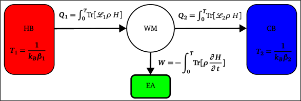
Figure 1: Basic diagram of a QTM: a hot bath (HB) at temperature $T_{1}$ and a cold batch (CB) at temperature $T_{2}$ exchange heat with the working medium (WM). This can also exchange work with an external agent (EA). The equations are the expressions for the heats and work assuming a Markovian master equation (see text). The directions of the arrows suggest a heat engine operation mode: $Q_{1}>0$ (the WM receives heat from the hot bath), $Q_{2}<0$ (the WM gives away part of that heat to the cold bath), and $W>0$ (the remaining heat is transformed into output work on the EA).

The suitable framework to describe the operation of QTMs is the theory of open quantum systems [28, 29]. In this framework, the working fluid is the only piece of a QTM that is explicitly accounted for; the heat reservoirs constitute the environment that is factored out, whereas the external agent that gives or receives work is only included as a normally time-dependent part of the Hamiltonian of the working fluid. Hereafter, we will furthermore assume the Markovian approximation, which can be used if certain conditions are met: essentially, the reservoir correlation times must be much shorter than the relaxation time of the system, and the system-bath interactions must be weak. The most general form for the equation of motion of an open system – the so-called master equation – in the Markovian approximation was demonstrated to be the Gorini-Kossakowski-Sudarshan-Lindblad (GKSL) form [30, 31]. In its original formulation, it accounted only for static Hamiltonians, but it can be extended to the time-dependent case. If the time-dependence is periodic, the master equation is often called “Floquet-Lindblad” equation [32, 33, 34]:

$$\dot{\rho}(t)=\mathcal{L}(f(t))\rho(t)\,.$$ (1)

Here, the Lindbladian time-dependence is assumed to be determined by the functions $f(t)$, a set of $m$ time-periodic functions of time,

$$f_{k}(t+T)=f_{k}(t),\;(k=0,1,\dots,m-1)\,,$$ (2)

with period $T$, that permit to control the precise form of the Lindbladian $\mathcal{L}$. The system is in contact with a number (normally, two) of heat reservoirs at different temperatures, and therefore we split $\mathcal{L}$ as:

$$\mathcal{L}(f(t))=\mathcal{L}_{H}(f(t))+\sum_{b}\mathcal{L}_{b}(f(t))\,,$$ (3)

where

$$\mathcal{L}_{H}(f(t))X=-i\left[H(f(t)),X\right]$$ (4)

is the unitary or coherent part of the time-evolution generator, whereas each $\mathcal{L}_{b}(f(t))$ is an incoherent operator that determines the interaction of the system with reservoir $b$.

The Hamiltonian $H(f(t))$ would generate the isolated evolution – although, in the presence of the environment terms, it should also include Lamb-shift terms that would be absent in isolation, and can be ignored in the weak coupling limit. Some of the terms of $H(f(t))$ may be time-dependent, controlled by some of the functions $f(t)$: those are the drivings originated by the external agent. Likewise, the interaction between the system and the reservoirs may also depend on some of the functions $f(t)$, allowing for example for the switching on and off of cold or hot baths, etc.

In the presence of both the periodic drivings and of the baths, under rather general assumptions [35], the system will eventually decay into a periodic NESS:

$$\rho(t+T)=\rho(t)\,.$$ (5)

This can then be viewed as a quantum thermal machine that performs a cycle of period $T$, giving and receiving energy into and from the baths (heat), and giving or receiving energy into and from the source of the external driving (work).

The energy balance can be understood in terms of those concepts. Defining the instantaneous energy function as:

$$E(t)={\rm Tr}\left[\rho(t)H(f(u,t))\right]\,,$$ (6)

we must have, in the NESS, $E(T)=E(0)$. Following Alicki [36], the variation of this energy can be broken down as:

$$\frac{{\rm d}E}{{\rm d}t}(t)=-p(t)+\sum_{b}j_{b}(t)\,,$$ (7)

where:

$$j_{b}(t) ={\rm Tr}\left[\mathcal{L}_{b}(f(t))\rho(t)\;H(f(t))\right]\,,$$ (8)

$$p(t) =-{\rm Tr}\left[\rho(t)\frac{\partial H}{\partial t}(f(t))\right]\,.$$ (9)

These are the energy flows transferred to the system, per unit time, from the baths and to the external agent, i.e. the transferred heats and work, respectively (or, if the sign is negative, energies per unit time transferred to the baths or from the external agent). One may then define the amounts of heats and work over one cycle:

$$Q_{b}=\int_{0}^{T}\!\!{\rm d}t\;j_{b}(t)\,,$$ (10)

$$W=\int_{0}^{T}\!\!{\rm d}t\;p(t)\,.$$ (11)

Here, we will use these energies per unit time (i.e. with dimensions of power), $J_{b}=Q_{b}/T$, and $P=W/T$. Given the periodic behaviour of our system,

$$\int_{0}^{T}\!\!{\rm d}t\;\frac{{\rm d}E}{{\rm d}t}(t)=E(T)-E(0)=0\,.$$ (12)

we must have an energy balance that is usually presented as the formulation of the I Law of thermodynamics for QTMs:

$$P=\sum_{b}J_{b}\,.$$ (13)

3 Floquet-engineering QTMs

The goal now is to find those control functions $f$ that lead the QTM to work in an optimal regime. The definition of what “optimal” means may of course vary. For example, one may wish to maximise the power output of a quantum engine, its efficiency, or the coefficient of performance of a refrigerator. In general, the goals would probably be functions of the energy terms $J_{b}$ and $P$ defined above.

Rather than working with unconstrained functions of time, it is more convenient to parameterise these functions,

$$f_{k}=f_{k}(u^{(k)},t)\quad(k=0,\dots,m-1)\,,$$ (14)

where each $u^{(k)}$ is a set of control parameters, that we collectively group into $u$ to ease the notation, as we collectively group all $f_{k}$ into the multi-dimensional function $f$. In this way, it is much easier to constrain the functions to experimentally or physically meaningful forms (in terms of frequencies, amplitudes, etc.) Therefore, the task is to find the optimal set of control parameters $u^{\rm opt}$ that lead to forms for the functions $f$ that optimise the machine behaviour.

We will hereafter denote $\rho(u,t)$ to the periodic solution (NESS) of the master equation:

$$\dot{\rho}(u,t) =\mathcal{L}(f(u,t))\rho(u,t)\,.$$ (15)

$$\rho(u,t+T) =\rho(u,t)$$ (16)

The optimisation problem must be formulated by establishing first the goal: a functional of the behaviour of the system during one cycle,

$$F=F(\rho,u)\,,$$ (17)

where the $\rho$ dependence refers to the full periodic trajectories in the cycle. The extra dependence on $u$ may be used to add penalties over undesirable regions of parameter space (an example of this will be given later).

The goal is therefore to maximise function

$$G(u)=F(\rho(u,\cdot),u)\,,$$ (18)

where now $\rho(u,\cdot)$ denotes the particular periodic trajectory that is the NESS solution to Eqs. (15) and (16).

In order to solve this optimisation problem, the first ingredient is therefore a computational procedure to obtain the NESS $\rho(u,\cdot)$, and function $G(u)$ from it. Numerous optimisation methods exist that permit to obtain optimal values for functions with only that ingredient. However, more effective methods can be used if one also has a procedure to compute the gradient of $G$. By applying the chain rule for functional derivatives in order to get an expression for this gradient,

$$\frac{\partial G}{\partial u_{r}}(u) =\frac{\delta F}{\delta\rho}(\rho(u,\cdot),u)\left(\frac{\partial\rho}{\partial u_{r}}(u,\cdot)\right)$$

$$+\frac{\delta F}{\delta\rho^{*}}(\rho(u,\cdot),u)\left(\frac{\partial\rho^{*}}{\partial u_{r}}(u,\cdot)\right)$$

$$+\frac{\partial F}{\partial u_{r}}(\rho(u,\cdot),u)\,,$$ (19)

it becomes clear that the second necessary ingredient for the optimisation of $G$ involves the computation of the gradient of $\rho(u,\cdot)$ with respect to the control parameters $u$.

In Ref. [24], we demonstrated the feasibility of a computational procedure to obtain these derivatives, and consequently, the feasibility of a procedure for the optimisation of function $G$. In that work, it was limited to functionals $F$ defined as averages of observables, i.e.:

$$F(\rho,u)=\frac{1}{T}\int_{0}^{T}\!\!{\rm d}t\;{\rm Tr}\left[A\rho(u,t)\right]\,,$$ (20)

although it can be extended to more general cases – for example, functions of the heats and power flowing to and from a QTM, as it will shown below.

Let us start by briefly summarising the procedure used in [24] to obtain the NESS and its gradient with respect to the control parameters. The starting point are the Floquet-Lindblad equations (15-16) in the frequency domain – a transformation using Fourier series that will automatically imply the periodicity of all the objects:

$$\sum_{\beta}\sum_{p=0}^{N-1}\left[\mathcal{L}_{\alpha\beta,q-p}(u)-i\delta_{pq}\delta_{\alpha\beta}\omega_{p}\right]\tilde{\rho}_{\beta,p}(u)=0\quad(q=0,1,\dots,N-1).$$ (21)

Here, $\omega_{p}=\frac{2\pi}{T}p\;(p\in\mathbb{Z})$ are the Fourier expansion frequencies, $N$ is the integer that sets a cutoff for the Fourier expansion, and

$$\tilde{\rho}_{\beta,p}(u) = \frac{1}{T}\int_{0}^{T}\!\!{\rm d}t\;e^{-i\omega_{p}t}\rho_{\alpha}(u,t),$$ (22)

$$\mathcal{L}_{\alpha\beta,q}(u) = \frac{1}{T}\int_{0}^{T}\!\!{\rm d}t\;e^{-i\omega_{q}t}\mathcal{L}_{\alpha\beta}(u,t),$$ (23)

are the Fourier coefficients of the elements of the density matrix and Lindbladian. Note that we are using here a vectorized representation of the density (a vector in Liouville space): the indices $\alpha$ or $\beta$ run over the $d^{2}$ elements of the density matrix ($d$ being the dimension of the underlying Hilbert space of the working fluid). The Lindbladian is then a rank two operator in Liouville space or superoperator and requires two indices, $\alpha\beta$.

By further defining

$$\overline{\mathcal{L}}_{\alpha q,\beta p}(u)=\mathcal{L}_{\alpha\beta,q-p}(u)-i\delta_{qp}\delta_{\alpha\beta}\omega_{p}\,,$$ (24)

we finally arrive to:

$$\sum_{\beta}\sum_{p=0}^{N-1}\overline{\mathcal{L}}_{\alpha q,\beta p}(u)\tilde{\rho}_{\beta,p}(u)=0\,,$$ (25)

or

$$\overline{\mathcal{L}}(u)\tilde{\rho}(u)=0\,.$$ (26)

in matrix form. Note that the dimension of vector $\tilde{\rho}$ is $d^{2}N$, and the operator $\overline{\mathcal{L}}(u)$ is a $d^{2}N\times d^{2}N$ matrix.

This is a linear homogeneous equation; the solution (the nullspace or kernel, assuming that it has dimension one), will be the periodic solution that we are after, the NESS. We now need some procedure to find $\frac{\partial\rho}{\partial u_{r}}$. Taking variations of Eq. (25) with respect to the parameters $u$, we get:

$$\overline{\mathcal{L}}(u)\frac{\partial\tilde{\rho}}{\partial u_{r}}(u)=-\frac{\partial\overline{\mathcal{L}}}{\partial u_{r}}(u)\tilde{\rho}(u).$$ (27)

This is a linear equation that would provide $\frac{\partial\tilde{\rho}}{\partial u_{r}}$. However, note that since $\overline{\mathcal{L}}(u)$ has a non-empty kernel (given precisely by $\tilde{\rho}(u)$), it cannot be solved straightforwardly. In fact, it does not have a unique solution: If $x$ is a solution of

$$\overline{\mathcal{L}}(u)x=-\frac{\partial\overline{\mathcal{L}}}{\partial u_{r}}(u)\tilde{\rho}(u),$$ (28)

$x+\mu\tilde{\rho}(u)$ is also a solution for any $\mu$. To remove this arbitrariness, we impose the normalisation condition, ${\rm Tr}\rho(u)=1$ for any $u$, and therefore:

$${\rm Tr}\frac{\partial\rho}{\partial u_{r}}=0.$$ (29)

To find $\frac{\partial\rho}{\partial u_{r}}$ in practice, one may then take the following two steps: First, compute a solution of the linear equation, Eq. (28), with the least-squares method, by imposing that the solution $x_{0}$ is perpendicular to the kernel, i.e.: $x_{0}^{\dagger}\cdot\tilde{\rho}(u)=0$. Then, update the solution with the condition, Eq. (29). The required solution is obtained as:

$$\frac{\partial\rho}{\partial u_{r}}=x_{0}-({\rm Tr}x_{0})\rho(u).$$ (30)

Once we have $\frac{\partial\rho_{u}}{\partial u_{r}}$, we can evaluate the gradient in Eq. (19). Armed with this procedure to compute this gradient, one can perform the optimisation of function $G(u)$ with many efficient algorithms. This method has been implemented in the qocttools code [37], publicly available, and all the necessary scripts and data necessary to replicate the following results are also available upon request from the authors.

As for possible choices for the function $G(u)$, for the purposes of this work, we are concerned with target goals defined in terms of either the averaged power $P$ or the heats $J_{b}$ (or combinations of those). For example, if the goal is to maximise the output power of a heat engine,

$$G(u)=P(u) =-\frac{1}{T}\int_{0}^{T}\!\!{\rm d}t\;{\rm Tr}\left[\frac{\partial H}{\partial t}(f(u,t))\rho(u,t)\right]\,,$$

$$=-\frac{1}{T}\sum_{k}\int_{0}^{T}\!\!{\rm d}t\;\dot{f}_{k}(u,t){\rm Tr}\left[V_{k}(f(u,t))\rho(u,t)\right]\,.$$ (31)

Note the negative sign due to the convention used for the definition of the power $P$. Here, we use the notation $\dot{f}_{k}(u,t)$ for the time derivative of function $f_{k}(u,t)$), and

$$V_{k}=\frac{\partial H}{\partial f_{k}}\,.$$ (32)

One must now work out the gradient of this function, for example making use of the chain rule (19), plugging the gradient $\frac{\partial\rho}{\partial u_{r}}$ calculated with the procedure described above. Rather than working out explicitly the functional derivatives, one may work out directly the gradient components of function $P(u)$ from Eq. (31):

$$\frac{\partial P}{\partial u_{r}}(u)= -\frac{1}{T}\sum_{k}\int_{0}^{T}\!\!{\rm d}t\;\left\{\frac{\partial\dot{f}_{k}}{\partial u_{r}}(u,t){\rm Tr}\left[V_{k}(f(u,t))\rho(u,t)\right]+\right.$$

$$\sum_{l}\dot{f}_{k}(u,t)\frac{\partial f_{l}}{\partial u_{r}}(u,t){\rm Tr}\left[\frac{\partial V_{k}}{\partial f_{l}}(f(u,t))\rho(u,t)\right]+$$

$$\left.\dot{f}_{k}(u,t){\rm Tr}\left[V_{k}(f(u,t))\frac{\partial\rho}{\partial u_{r}}(u,t)\right]\right\}\,.$$ (33)

Despite the length of the equation, in fact the main difficulty lies in computing the NESS $\rho(u,t)$ and its derivatives $\frac{\partial\rho}{\partial u_{r}}$.

A similar procedure can be followed for the case in which function $G(u)=J_{b}(u)$, the heat transferred from one of the reservoir. In the most general case, function $G$ would be a function of all the energy terms, $G(u)=g(P(u),J_{1}(u),\dots)$, a function of the power output and of all the heats (such as the efficiency of a heat engine or the coefficient of performance of a refrigerator), and then one would have:

$$\frac{\partial G}{\partial u_{r}}=\frac{\partial g}{\partial P}\frac{\partial P}{\partial u_{r}}+\sum_{b}\frac{\partial g}{\partial J_{b}}\frac{\partial J_{b}}{\partial u_{r}}\,.$$ (34)

4 Examples of application

4.1 GKSL equations

Until now, the form of the master equation has remained rather general – although we are always assuming here an important simplification: the open quantum system is Markovian. Therefore, the equation must be of the GKSL form [30, 31]. The optimisation method described above may be used for any equation of that family. However, it has only been implemented and tested for a subclass of GKSL equations: hereafter, in order to exemplify the method, we will restrict the analysis to those GKSL equations that verify:

1. The decoherence terms have the form:

   $$\mathcal{L}_{b}(f(u,t))=\sum_{i}g_{bi}(f(u,t))L_{D}(\gamma_{bi},L_{bi})\,.$$ (35)

   where we define the super-operator $L_{D}(\gamma,X)$ (for any positive constant $\gamma$ and operator $X$) as:

   $$L_{D}(\gamma,X)\rho=\gamma\left(X\rho X^{\dagger}-\frac{1}{2}\left\{X^{\dagger}X,\rho\right\}\right)\,.$$ (36)

   Therefore, in this setup, we restrict the Lindblad operators $L_{bi}$ to be constant in time, but they may be modulated by time-dependent functions (the so-called “rates” may depend on time).

2. We have two reservoirs at thermal equilibrium (as it is almost always the case): one hot bath $(b=1)$ and one cold bath $(b=2)$.

3. The dependence of H on the control functions is linear, i.e.:

   $$H(f(u,t))=H_{0}+\sum_{k}f_{k}(u,t)V_{k}\,.$$ (37)

   and therefore the terms $V_{k}$ are constant operators, independent of $u$ or time.

This is the type of model that has been implemented in the qocttools code [37] to demonstrate the feasibility of the optimisation scheme explained above. The key equations are two: on the on hand, the expression for the gradient, that in this case reduces to:

$$\frac{\partial P}{\partial u_{r}}(u)=-\frac{1}{T}\sum_{k}\int_{0}^{T}\!\!{\rm d}t\;\left\{\frac{\partial\dot{f}_{k}}{\partial u_{r}}(u,t){\rm Tr}\left[V_{k}\rho(u,t)\right]+\dot{f}_{k}(u,t){\rm Tr}\left[V_{k}\frac{\partial\rho}{\partial u_{r}}(u,t)\right]\right\}\,.$$ (38)

And, in order to find the gradient of $\rho$ [Eq. (27)], since

$$\frac{\partial\overline{\mathcal{L}}}{\partial u_{r}}=\sum_{k}\frac{\partial\overline{\mathcal{L}}}{\partial f_{k}}\frac{\partial f_{k}}{\partial u_{r}}\,,$$ (39)

the key equation is:

$$\frac{\partial\mathcal{L}}{\partial f_{k}}=-i\left[V_{k},\cdot\right]+\sum_{b}\sum_{i}\frac{\partial g_{bi}}{\partial f_{k}}(f(u,t))L_{D}(\gamma_{bi},L_{bi})\,.$$ (40)

4.2 Model

Let us now present the model used for the sample optimisations shown below. We consider the model used by Erdman et al. [15] to study the optimal Otto cycles (see also [38, 16, 17]): a two level system with a controlled energy gap, i.e.:

$$H(f(t))=\frac{1}{2}(\Delta+f_{0}(t))\sigma_{z}\,.$$ (41)

Note that in this subsection 4.2 we are dropping the dependence on $u$ to ease the notation.

Regarding the decoherence terms [Eq. (35)], there are two terms per bath, indexed as $i=+,-$, and

$$L_{b+}=\sigma_{+}\,,\;\;L_{b-}=\sigma_{-}\,,$$ (42)

for both the hot and cold bath ($b=1,2$). All rate constants $\gamma_{bi}$ are set to be equal ($\gamma_{bi}=\Gamma$), but they are then modulated by the time-dependent functions

$$g_{bi}(f(t))=f_{b}(t)F(i\beta_{b}(\Delta+f_{0}(t)))\,.$$ (43)

where $\beta_{b}$ is the (inverse) temperature of bath $b$, and

$$F(x)=\frac{1}{1+e^{x}}\,.$$ (44)

This choice ensures the fulfillment of the detailed balance condition.

Note that we have three control functions: $f_{0}(t)$ is responsible for modifying the TLS gap, whereas $f_{1}(t)$ and $f_{2}(t)$ tune the coupling of the system to the hot and cold bath, respectively.

This model has been used to describe a quantum dot with only one relevant resonance, coupled to metallic leads with flat densities of states, that act as reservoirs [39, 38, 15, 16]. Erdman et al. [15], in particular, solved exactly and analytically the following optimisation problem: suppose that we can vary at will the TLS gap by modulating $f_{0}$, as long as a maximum and a minimum are not surpassed: $|f_{0}(t)|\leq\delta$. This means there exists a minimum and a maximum TLS gap:

$$\varepsilon_{\rm min}(=\Delta-\delta)\leq\Delta+f_{0}(t)\leq\varepsilon_{\rm max}(=\Delta+\delta)\,.$$ (45)

Suppose that we can also vary at will the system-bath coupling functions $f_{1}$ and $f_{2}$, as long as $0\leq|f_{b}(t)|\leq 1$. All these control functions are periodic, with a period $T$ that can also be varied. Suppose now that we want to optimize the output power of the QTM operating as heat engine (other possible performance measures were also considered in [15]).

The solution was demonstrated to be the following (see the discussion about the Eq. (8) of [15]): the maximum is achieved with infinitesimally short ($T\to 0$) periods, consisting of coupling the system for equal periods of time ($T/2$) to the hot and the cold baths:

$$f_{1}(t)=1\;\;\textrm{and}\;\;f_{2}(t)=0\;\;\textrm{if}\;\;0\leq t\leq\frac{T}{2}\;\;\; \textrm{(coupling to the hot bath)}\,,$$ (46)

$$f_{1}(t)=0\;\;\textrm{and}\;\;f_{2}(t)=1\;\;\textrm{if}\;\;\frac{T}{2}\leq t\leq T\;\;\; \textrm{(coupling to the cold bath)}\,.$$ (47)

During each of those strokes, the TLS gap has some constant values, $\varepsilon_{1}$ and $\varepsilon_{2}$, respectively. In this setup, the output power is given by:

$$P_{\rm c}(T,\varepsilon_{1},\varepsilon_{2})=\frac{1}{\Gamma\textbf{coth}(\Gamma\frac{T}{4})}(F(\varepsilon_{1}\beta_{1})-F(\varepsilon_{2}\beta_{2}))(\varepsilon_{1}-\varepsilon_{2})\,,$$ (48)

where the subindex ${\rm c}$ stands for “constant”, to stress the fact that the function $f_{0}(t)$ is constant during each time of contact with the bath: $f_{0}(t)=\epsilon_{b}-\Delta$ when in contact with bath $b$, and it changes value instantaneously when the bath changes. The value of this output power grows with decreasing periods $T$; in the limit $T\to 0$,

$$P_{\rm c}(\varepsilon_{1},\varepsilon_{2})=\frac{\Gamma}{4}(F(\varepsilon_{1}\beta_{1})-F(\varepsilon_{2}\beta_{2}))(\varepsilon_{1}-\varepsilon_{2})\,.$$ (49)

The absolute maximum output power for this type of machine is then found at the maximum of this function:

$$P_{\rm c}^{\rm max}=\max_{\varepsilon_{\rm min}\leq\varepsilon_{1},\varepsilon_{2}\leq\varepsilon_{\rm max}}P_{\rm c}(\varepsilon_{1},\varepsilon_{2})\,.$$ (50)

This can be viewed as a two-strokes Otto cycle, that switches discontinuously from the cold to the hot bath, with no adiabatic segments. The expansion and compressions (modifications of the TLS gap, in this case), are instantaneous. Therefore, even at finite $T$, the operation requires discontinuous jumps in the control functions.

4.3 Examples of optimizations

Let us now modify the nature of the problem described above: suppose that we are not allowed to use a non-smooth control function $f_{0}$: the change in time of the TLS gap cannot be sudden, which implies a continuous and differentiable function $f_{0}$. We still ask of $f_{0}$ to be constrained in amplitude, $|f_{0}(u,t)|\leq\delta$, as mentioned above, but also demand that it has no frequency components beyond a cutoff $\omega_{\rm max}$. This cutoff forbids, of course, a sudden discontinuous change when the system decouples from one bath and couples to the other one. Furthermore, we fix the cycle period $T$, which in a realistic setup cannot be taken to arbitrarily close-to-zero values.

The rest of the setup remains unchanged: $f_{1}$ and $f_{2}$ are given by Eqs. (46) and (47), which means that once again we have a two-stroke cycle that switches the contact from the hot bath to the cold bath. We therefore consider these functions to be fixed: they do not depend on any control parameters $u$ and are not, in purity, control functions. The optimisation is only done with respect to the shape of $f_{0}=f_{0}(u,t)$ (this is of course not a requirement of the method, but merely a choice for the examples shown here).

Regarding the parameterisation of $f_{0}$, it is chosen in such a way that, by definition, $|f_{0}(u,t)|\leq\delta$ as in the problem described above. Furthermore, the function is periodic, continuous and differentiable, and has low frequencies. The detailed description of the parameterised form of $f_{0}$ is given in Appendix A.

It remains to define the merit function $G$ for this example, which is:

$$G(u)=P(u)-\alpha\sum_{\omega_{k}>\omega_{\rm max}}|\tilde{f}_{0k}(u)|^{2}\,.$$ (51)

The goal is therefore to maximise the output power $P(u)$ as given by Eq. 31; but note that we add an extra term: it is a penalty term for high frequencies in the control function ($\tilde{f}_{0k}(u)$ are the Fourier components of $f_{0}$). As discussed in Appendix A, the parameterisation forbids amplitudes higher than $\delta$, and favours frequencies lower than $\omega_{\rm max}$, but does not forbid them. Therefore, in the optimisation we add this extra term to make them negligible. The constant $\alpha>0$ determines how important this penalty is, and therefore how large those frequencies can be in the resulting optimised function.

Then, the function $P$ and its gradient are computed according to the formulas described in the previous section, and this information is fed into an optimisation algorithm. We have chosen the sequential quadratic programming algorithm for nonlinearly constrained gradient-based optimisation (SLSQP) [40], as implemented in the NLopt library [41]. This is a versatile choice that permits to include linear and non-linear bounds and constraints.

For all the calculations shown below, the amplitude constraint is set as $\delta=(1/5)\Delta$ and the temperatures for the reservoirs are set to $\beta_{1}=1/\Delta$, $\beta_{2}=2/\Delta$, and the rate $\Gamma=\Delta$, equal for all the dissipation terms.

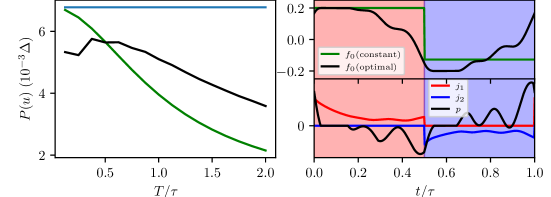
Figure 2: Left panel: Averaged output power of the heat engine as a function of the period time $T$ when using the: green: constant TLS gaps with discontinous fast switching when changing bath; and black: optimized smooth gap $f_{0}(u^{\rm opt},t)$. The theoretical optimal limit using an infinitely fast-switching protocol is also shown in blue. Top right panel: Function $f_{0}$ with constant TLS gaps and sudden switching (green), and optimized $f_{0}(u^{\rm opt},t)$. The red and blue shadings mark the time regions when the hot and blue baths are connected, respectively. Bottom right panel: Transferred heats and work for the heat engine when using $f_{0}(u^{\rm opt},t)$.

Fig. 2 displays the first calculation examples. It is a series of optimisations for varying values of the cycle period $T$, ranging from $(1/8)\tau$ to $2\tau$, where $\tau=\frac{2\pi}{\Delta}$. The goal is to optimise the output power obtained with a protocol $f_{0}(u,t)$ for each of those cycle periods, and compare that output power with the one that results of using constant TLS gaps during each contact with the hot and cold bath, with a sudden, instantaneous change in between. The output power obtained with those constant gaps is the one obtained by maximising Eq. 48 with respect to $\varepsilon_{1}$ and $\varepsilon_{2}$ (within the allowed range $[\Delta-\delta,\Delta+\delta]$). The results are shown in the left panel of Fig. 2. The green line displays the output power obtained with the constant gaps; it can be seen how it increases with decreasing $T$, and it tends to the maximum predicted by Eq. 49 (shown with the blue line in Fig. 2), as expected.

However, for a fixed and non-zero $T$, the values obtained with constant gaps are not the largest output powers that one can get; in order to find the optimal protocol, one must look in the space of non-constant, varying TLS gaps, for which purpose one has to use a numerical procedure such as the one proposed in this work. The results obtained in this way are shown with the black line of the left panel of Fig. 2. It can be seen how, for small $T$, the output powers are actually lower, and only become larger at a certain crossing point. The reason is the fact that we are demanding of the protocol to have frequencies lower than a certain cutoff (which for these examples we have set to $\omega_{\rm max}=8\Delta$). It is therefore not surprising that, for very rapid cycles, the optimised $f_{0}$ cannot improve the constant-gap protocol, that approaches the predicted absolute maximum as $T\to 0$. For longer cycles, the black curve does show higher output powers.

The right panel of Fig. 2 presents the optimal function $f_{0}(u^{\rm opt},t)$ (top) and the corresponding transferred heats and work (bottom) corresponding to the heat engine working with a period of $T=\tau$. For comparison, the protocol using the optimised constant gaps is also shown in the top panel (green line). It can be seen how, as expected, the energy exchange between system and external agent is higher around the times that the baths are coupled and decoupled. The optimised function $f_{0}$ does fulfil the required constraints regarding amplitude and frequency.

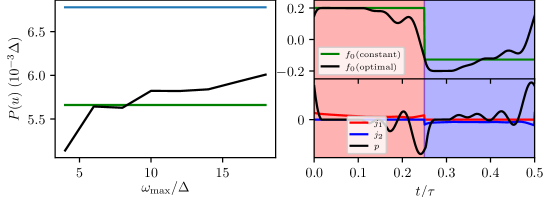
Figure 3: Left panel: Optimized averaged output power of the heat engine as a function of the cutoff $\omega_{\rm max}$ (black curve). The theoretical optimal limit using an infinitely fast-switching protocol is shown in blue; whereas the value obtained when using constant TLS gaps with discontinous fast switching is also shown in green. Top right panel: Function $f_{0}$ with constant TLS gaps and sudden switching (green), and optimized $f_{0}(u^{\rm opt},t)$. The red and blue shadings mark the time regions when the hot and blue baths are connected, respectively. Bottom right panel: Transferred heats and work for the heat engine when using $f_{0}(u^{\rm opt},t)$.

The results shown in Fig 2 – in particular, how the optimised $f_{0}$ cannot improve the constant gap protocol for very short $T$ – point to the relevance of the choice of the cutoff. To illustrate this fact, we will show the effect of the cutoff in Fig. 3. In this case, the series of runs were done fixing $T=\frac{1}{2}\tau$, but changing the value of the cutoff frequency, from $\omega_{\rm max}=4\Delta$ to $\omega_{\rm max}=18\Delta$. Increasing the cutoff frequency amounts to enlarging the search space for the optimisation, and therefore it can be seen on the left panel how the output power obtained with the optimised $f_{0}$ increases with $\omega_{\rm max}$. For lower cutoffs, it cannot improve over the value obtained with the constant gap protocol, but for larger cutoffs the time-varying optimised $f_{0}$ permits to obtain a better number, reflecting the fact that the value obtained with constant gaps is only a maximum in the limit $T\to 0$. Finally, on the right hand side of Fig. 3 we display again function $f_{0}(u^{\rm opt},t)$ (top), and the instantaneous heats and work (bottom), in this case for the calculation with $\omega_{\max}=18\Delta$. Function $f_{0}$ changes more rapidly as a function of time than in the case shown in Fig. 2, but it still respects the constrains imposed on the amplitude and the frequency.

5 Conclusion

This work describes and demonstrates a procedure for the optimisation of the working protocol of QTMs modelled with generic Markovian master equations. Although there have been numerous works dealing with the theoretical problem of establishing optimal performance limits for these systems, there have been few practical, computational methods proposed in the literature focused on finding realistic optimal protocols for the action of the external agent or the couplings to the baths. Specially, if one assumes that ideal unconstrained modes or operation are not feasible, and bounds on the smoothness or amplitudes of the control functions are to be considered, based on experimental or physical considerations. This work intends to fill in that gap.

As a demonstration, we have computed optimised protocols for two-level systems coupled to thermal reservoirs, that may be for example used to model simple quantum dots coupled to metallic leads at varying temperatures. These can operate as minimal Otto quantum heat engines, producing output power through the intermittent switch from the cold to the hot bath. The action of the external agent is given by the gap of the TLS, and it is the shape of this function the one that, in the example shown, is controlled. It is shown how this function can be parameterised respecting amplitude and frequency constraints, and how the value of those parameters can be efficiently optimised using a gradient-based algorithm. The method can also be used to optimise the functions controlling the couplings to the baths, internal bath parameters such as their temperatures if one considers them to be time-dependent, the duration of the cycle or of each bath coupling, etc.

There has been a recent push in the research of QTMs, motivated by the technological and experimental trend towards the miniaturisation of devices, and by the theoretical questions around the interplay of thermodynamics for mesoscopic systems and quantum mechanics. I expect that the method proposed here, and the code that implements it (published as open source), will be useful to analyse the performance of these systems.

Appendix A Parametrization of the control function

Function $f_{0}(u,t)$ should fulfill two conditions that would normally be present in any experimental implementation of a QTM. First, it must be bound: $|f_{0}(u,t)|\leq\delta$. Second, it should be smooth, which we will enforce by also requiring a high-frequency cutoff. This suggests the following parametrization:

$$f_{0}(u,t)=\Phi(f_{\rm Fourier}(u,t))\,.$$ (A.1)

Here, the parameters $u$ are the coefficients of a Fourier series:

$$f_{\rm Fourier}(u,t)=u_{0}+\sum_{n=1}^{M}\left(u_{2n}\cos(\omega_{n}t)+u_{2n-1}\sin(\omega_{n}t)\right),\quad(\omega_{n}=\frac{2\pi}{T}n)\,.$$ (A.2)

The function $\Phi$ is chosen with the following properties: (i) for small $x$, $\Phi(x)\approx x$. Therefore, if $f_{\rm Fourier}(u,t)$ is small, $f_{0}(u,t)$ is simply equal to a Fourier series with a frequency cutoff, $f_{\rm Fourier}(u,t)$. (ii) as $|x|$ grows and approaches $\delta$, the growth of $|\Phi(x)|$ is reduced, so that $|\Phi(x)|\leq\delta$ for any $x$, until it becomes a constant equal to $\delta$ for $x>\delta$.

Many possible functions can be imagined with those properties. For this work, we have chosen:

$$\Phi(x)=\left\{\begin{array}[]{l}x\quad\textrm{ if }0\leq x\leq\frac{3}{4}\delta\\ \delta\quad\textrm{ if }x\geq\delta+\frac{1}{4}\delta\\ \textrm{an Akima cubic spline interpolation if }x\in(\frac{3}{4}\delta,\delta+\frac{1}{4}\delta)\end{array}\right.$$ (A.3)

For $x<0$, the function should be antisymmetric: $\Phi(x)=-\Phi(-x)$.

This parameterisation strictly enforces the amplitude bound $|\Phi(x)|\leq\delta$, but it does not enforce the frecuency cutoff; it only favours the frequencies lower then $\omega_{\rm max}$, as long as the value of the coefficients $u$ are not high.

References

- [1] H. E. D. Scovil and E. O. Schulz-DuBois, Three-level masers as heat engines, Phys. Rev. Lett. 2, 262 (1959), 10.1103/PhysRevLett.2.262.
- [2] S. Bhattacharjee and A. Dutta, Quantum thermal machines and batteries, The European Physical Journal B 94(12), 239 (2021), 10.1140/epjb/s10051-021-00235-3.
- [3] R. Alicki and D. Gelbwaser-Klimovsky, Non-equilibrium quantum heat machines, New Journal of Physics 17(11), 115012 (2015), 10.1088/1367-2630/17/11/115012.
- [4] V. Blickle and C. Bechinger, Realization of a micrometre-sized stochastic heat engine, Nature Physics 8(2), 143 (2012), 10.1038/nphys2163.
- [5] O. Abah, J. Roßnagel, G. Jacob, S. Deffner, F. Schmidt-Kaler, K. Singer and E. Lutz, Single-ion heat engine at maximum power, Phys. Rev. Lett. 109, 203006 (2012), 10.1103/PhysRevLett.109.203006.
- [6] J. Roßnagel, S. T. Dawkins, K. N. Tolazzi, O. Abah, E. Lutz, F. Schmidt-Kaler and K. Singer, A single-atom heat engine, Science 352(6283), 325 (2016), 10.1126/science.aad6320.
- [7] D. von Lindenfels, O. Gräb, C. T. Schmiegelow, V. Kaushal, J. Schulz, M. T. Mitchison, J. Goold, F. Schmidt-Kaler and U. G. Poschinger, Spin heat engine coupled to a harmonic-oscillator flywheel, Phys. Rev. Lett. 123, 080602 (2019), 10.1103/PhysRevLett.123.080602.
- [8] J. P. S. Peterson, T. B. Batalhão, M. Herrera, A. M. Souza, R. S. Sarthour, I. S. Oliveira and R. M. Serra, Experimental characterization of a spin quantum heat engine, Phys. Rev. Lett. 123, 240601 (2019), 10.1103/PhysRevLett.123.240601.
- [9] J. Klatzow, J. N. Becker, P. M. Ledingham, C. Weinzetl, K. T. Kaczmarek, D. J. Saunders, J. Nunn, I. A. Walmsley, R. Uzdin and E. Poem, Experimental demonstration of quantum effects in the operation of microscopic heat engines, Phys. Rev. Lett. 122, 110601 (2019), 10.1103/PhysRevLett.122.110601.
- [10] M. H. M. Passos, A. C. Santos, M. S. Sarandy and J. A. O. Huguenin, Optical simulation of a quantum thermal machine, Phys. Rev. A 100, 022113 (2019), 10.1103/PhysRevA.100.022113.
- [11] F. Binder, L. A. Correa, C. Gogolin, J. Anders and G. Adesso, eds., Thermodynamics in the Quantum Regime, Springer, https://doi.org/10.1007/978-3-319-99046-0 (2018).
- [12] F. Cleri, Quantum computers, quantum computing and quantum thermodynamics (2024), 2404.09663.
- [13] R. Kosloff, Quantum thermodynamics: A dynamical viewpoint, Entropy 15, 2100 (2013), 10.3390/e15062100.
- [14] S. Carnot, Réflexions sur la puissance motrice du feu et sur les machines propres a développer cette puissance, Bachelier, Paris (1824), http://catalogue.bnf.fr/ark:/12148/cb301979237.
- [15] P. A. Erdman, V. Cavina, R. Fazio, F. Taddei and V. Giovannetti, Maximum power and corresponding efficiency for two-level heat engines and refrigerators: optimality of fast cycles, New Journal of Physics 21(10), 103049 (2019), 10.1088/1367-2630/ab4dca.
- [16] P. A. Erdman and F. Noé, Identifying optimal cycles in quantum thermal machines with reinforcement-learning, npj Quantum Information 8(1), 1 (2022), 10.1038/s41534-021-00512-0.
- [17] P. A. Erdman, A. Rolandi, P. Abiuso, M. Perarnau-Llobet and F. Noé, Pareto-optimal cycles for power, efficiency and fluctuations of quantum heat engines using reinforcement learning, Phys. Rev. Res. 5, L022017 (2023), 10.1103/PhysRevResearch.5.L022017.
- [18] P. A. Erdman and F. Noé, Model-free optimization of power/efficiency tradeoffs in quantum thermal machines using reinforcement learning, PNAS Nexus 2(8), pgad248 (2023), 10.1093/pnasnexus/pgad248.
- [19] I. Khait, J. Carrasquilla and D. Segal, Optimal control of quantum thermal machines using machine learning, Phys. Rev. Res. 4, L012029 (2022), 10.1103/PhysRevResearch.4.L012029.
- [20] V. Cavina, A. Mari, A. Carlini and V. Giovannetti, Optimal thermodynamic control in open quantum systems, Phys. Rev. A 98, 012139 (2018), 10.1103/PhysRevA.98.012139.
- [21] L. S. Pontryagin, V. G. Boltyanskii, R. V. Gamkrelidze and E. F. Mishchenko, The Mathematical Theory of Optimal Processes, John Wiley & Sons (1962).
- [22] U. Boscain, M. Sigalotti and D. Sugny, Introduction to the Pontryagin Maximum Principle for quantum optimal control, PRX Quantum 2, 030203 (2021), 10.1103/PRXQuantum.2.030203.
- [23] G. N. Elnagar and M. A. Kazemi, Nonlinear periodic optimal control: A pseudospectral Fourier approach, Numerical Functional Analysis and Optimization 25(7-8), 707 (2005), 10.1081/NFA-200045793.
- [24] A. Castro and S. A. Sato, Optimizing Floquet engineering for non-equilibrium steady states with gradient-based methods, SciPost Physics 15, 029 (2023), 10.21468/SciPostPhys.15.1.029.
- [25] T. Oka and S. Kitamura, Floquet engineering of quantum materials, Annual Review of Condensed Matter Physics 10(Volume 10, 2019), 387 (2019), https://doi.org/10.1146/annurev-conmatphys-031218-013423.
- [26] A. Castro, U. De Giovannini, S. A. Sato, H. Hübener and A. Rubio, Floquet engineering the band structure of materials with optimal control theory, Phys. Rev. Research 4, 033213 (2022), 10.1103/PhysRevResearch.4.033213.
- [27] A. Castro, U. De Giovannini, S. A. Sato, H. Huebener and A. Rubio, Floquet Engineering with Quantum Optimal Control Theory, New Journal of Physics (2023), 10.1088/1367-2630/accb05.
- [28] H. P. Breuer and F. Petruccione, The Theory of Open Quantum Systems, vol. 9780199213, Oxford University Press, ISBN 978-0-19-170634-9, 10.1093/acprof:oso/9780199213900.001.0001 (2007).
- [29] R. Kosloff, A quantum mechanical open system as a model of a heat engine, The Journal of Chemical Physics 80(4), 1625 (1984), 10.1063/1.446862.
- [30] G. Lindblad, On the Generators of Quantum Dynamical Semigroups, Communications in Mathematical Physics 48(2), 119 (1976), 10.1007/BF01608499.
- [31] V. Gorini, A. Kossakowski and E. C. G. Sudarshan, Completely Positive Dynamical Semigroups of N-Level Systems, Journal of Mathematical Physics 17(5), 821 (1976), 10.1063/1.522979.
- [32] T. Mori, Floquet states in open quantum systems, Annual Review of Condensed Matter Physics 14(Volume 14, 2023), 35 (2023), https://doi.org/10.1146/annurev-conmatphys-040721-015537.
- [33] C. M. Dai, Z. C. Shi and X. X. Yi, Floquet theorem with open systems and its applications, Phys. Rev. A 93, 032121 (2016), 10.1103/PhysRevA.93.032121.
- [34] M. Hartmann, D. Poletti, M. Ivanchenko, S. Denisov and P. Hänggi, Asymptotic Floquet states of open quantum systems: the role of interaction, New Journal of Physics 19(8), 083011 (2017), 10.1088/1367-2630/aa7ceb.
- [35] P. Menczel and K. Brandner, Limit cycles in periodically driven open quantum systems, Journal of Physics A: Mathematical and Theoretical 52(43), 43LT01 (2019), 10.1088/1751-8121/ab435a.
- [36] R. Alicki, The quantum open system as a model of the heat engine, Journal of Physics A: Mathematical and General 12(5), L103 (1979), 10.1088/0305-4470/12/5/007.
- [37] A. Castro, qocttools: A program for quantum optimal control calculations, Computer Physics Communications 295, 108983 (2024), https://doi.org/10.1016/j.cpc.2023.108983.
- [38] P. A. Erdman, F. Mazza, R. Bosisio, G. Benenti, R. Fazio and F. Taddei, Thermoelectric properties of an interacting quantum dot based heat engine, Phys. Rev. B 95, 245432 (2017), 10.1103/PhysRevB.95.245432.
- [39] C. W. J. Beenakker, Theory of Coulomb-blockade oscillations in the conductance of a quantum dot, Phys. Rev. B 44, 1646 (1991), 10.1103/PhysRevB.44.1646.
- [40] D. Kraft, Algorithm 733: TOMP–Fortran modules for optimal control calculations, ACM Trans. Math. Softw. 20(3), 262–281 (1994), 10.1145/192115.192124.
- [41] S. G. Johnson, The NLopt nonlinear-optimization package, https://github.com/stevengj/nlopt (2007).