A regular center instead of a black bounce

S. V. Bolokhov,^a;1 K. A. Bronnikov,^a,b,c;2 and M. V. Skvortsova^a;3

^a

Institute of Gravitation and Cosmology, Peoples’ Friendship University of Russia (RUDN University),
ul. Miklukho-Maklaya 6, Moscow 117198, Russia

^b

Center for Gravitation and Fundamental Metrology, VNIIMS, Ozyornaya ul. 46, Moscow 119361, Russia

^c

National Research Nuclear University “MEPhI”, Kashirskoe sh. 31, Moscow 115409, Russia

The widely discussed “black-bounce” mechanism of removing a singularity at $r=0$ in a spherically symmetric space-time, proposed by Simpson and Visser, consists in removing the point $r=0$ and its close neighborhood, resulting in emergence of a regular minimum of the spherical radius that can be a wormhole throat or a regular bounce. Instead, it has been recently proposed to make $r=0$ a regular center by properly modifying the metric, still preserving its form in regions far from $r=0$. Different algorithms of such modifications have been formulated for a few classes of singularities. The previous paper considered space-times whose Ricci tensor satisfies the condition $R^{t}_{t}=R^{r}_{r}$, and regular modifications were obtained for the Schwarzschild, Reissner-Nordström metics, and two examples of solutions with magnetic fields obeying nonlinear electrodynamics (NED). The present paper considers regular modifications of more general space-times, and as examples, modifications with a regular center have been obtained for the Fisher (also known as JNW) solution with a naked singularity and a family of dilatonic black holes. Possible field sources of the new regular metrics are considered in the framework of general rlativity (GR), using the fact that any static, spherically symmetric metric with a combined source involving NED and a scalar field with some self-interaction potential. This scalar field is, in general, not required to be of phantom nature (unlike the sources for black bounces), but in the examples discussed here, the possible scalar sources are phantom in a close neighborhood of $r=0$ and are canonical outside it.

1 Introduction

The classical theories of gravity, beginning with general relativity (GR), in many of their most important solutions predict the emergence of space-time singularities that designate natural applicability limits of these theories. Since one can hardly believe in the reality of such formal inferences as infinite densities or curvatures, there have been many attempts to avoid such singularities thus making the theories universally applicable, still remaining in the framework of classical rather than quantum notions of space-time. Among them one can recall both low-energy or low-curvature limits of various models of quantum gravity [1, 2, 3, 4, 5, 6, 7, 8, 9, 10, 11] and application of geometries more general than Riemannian, including torsion, nonmetricity etc. or using gravitational theories more general than GR still using Riemannian geometry.

On the same trend, significant popularity was gained by simple phenomenological models of space-time that modify and regularize the Riemannian metric behavior in very strong field regions but almost preserve the geometry in the regions of weak or moderate curvature. This approach was probably used for the first time by J. Bardeen in 1968 [12], who proposed to consider, instead of the Schwarzschild line element, the regular black hole metric

$$ds^{2}=\bigg{(}1-\frac{2Mr^{2}}{(r^{2}+a^{2})^{3/2}}\bigg{)}dt^{2}-\bigg{(}1-\frac{2Mr^{2}}{(r^{2}+a^{2})^{3/2}}\bigg{)}^{-1}dr^{2}-r^{2}d\Omega^{2},\qquad d\Omega^{2}=d\theta^{2}+\sin^{2}\theta d\varphi^{2}.$$ (1)

This metric is defined in the range $r\geq 0$. At small values of the parameter $a$ relative to the Schwarzschild  mass $M$, which looks most natural ($a<a_{\rm crit}\approx 0.77M$), it describes a black hole with two horizons, at $a=a_{\rm crit}$ there is a single extremal horizon, and at $a>a_{\rm crit}$ horizons are absent, and we observe a soliton-like, or star-like geometry, and with any values of $a$ there is a regular center at the origin $r=0$. Similar properties are observed in Hayward’s metric [13] that differs from Bardeen’s by the replacement $(r^{2}+a^{2})^{3/2}\mapsto r^{3}+2M\ell^{2}$, $\ell={\rm const}$.

A great number of regular field models have been considered since then, even if we restrict our attention to static, spherically symmetric configurations.(see, e.g., [14, 15, 16] for recent reviews). Still, if our interest is not in regular geometries obtained directly but in regular models constructed, like (1), from singular ones by introducing a certain regularization parameter, we must above all pay attention to the metric proposed by Simpson and Visser (SV) [17] as a regular counterpart of the Schwarzschild space-tiime and its further generalizations [18, 19, 20] obtained from Reissner-Nordström and other singular static, spherically symmetric metrics. The way of converting a metric singular at $r=0$ to a regular one consists in replacing the spherical radius $r$ with the expression $r(u)=\sqrt{x^{2}+b^{2}}$, thus eliminating the singularity and its close neighborhood from space-time and smoothly joining its remaining part to one more copy of this part. In particular, the Schwarzschild metric is converted to [17]

$$ds^{2}=\bigg{(}1-\frac{2M}{x^{2}+a^{2}}\bigg{)}dt^{2}-\bigg{(}1-\frac{2M}{x^{2}+a^{2}}\bigg{)}^{-1}dx^{2}-(x^{2}+a^{2})d\Omega^{2}.$$ (2)

The resulting regular minimum of $r$ at $x=0$ is a wormhole throat if it occurs in a static region (it happens if $a^{2}>4M^{2}$, it is an extremal black hole horizon if $a^{2}=4M^{2}$, and if $a^{2}<4M^{2}$, it is a bounce of $r(x)$ as one of two cosmological scale factors in a Kantowski-Sachs anisotropic cosmology, where $x$ is a temporal coordinate. This region is located between two simple horizons $x=\pm\sqrt{4M^{2}-a^{2}}$. Such a bounce inside a black hole is called a black bounce according to [17], and all space-times constructed in this way are often called “black bounce space-times” or even simply “black bounces.” Numerous models found in this manner have gained much interest, such spherically symmetric geometries were generalized to include [21, 22, 23], there followed calculations of quasinormal modes, properties of gravitational waves and gravitational lensing in such space-times, etc. [25, 24, 26, 27, 28, 29, 30, 31, 32, 33, 34, 35, 36, 37, 38]. This whole trend may be regarded as one of simple ways to simulate possible effects of quantum gravity in the language of classical gravity, leaving aside any quantization details. The properties of new geometries constructed in this way may also be of certain interest. One can also note that black bounces as the phenomena of minimum $r(u)$ inside black holes have been found as quite a common feature in a number of solutions of GR and other theories in the presence of phantom scalar fields. Such space-times were called “black universes,” their black hole interior at times after a bounce becomes an expanding universe with isotropic (in particular, de Sitter) late-time asymptotic, see, e.g., [39, 40, 41, 42, 43, 44].

We can see that the basic feature of the black bounce concept is that a space-time singularity is cut away together with its close environment, and the resulting regular space-time is almost doubled as compared to the original one. There emerge new geometries and causal structures more complex than before, which may cause additional interest but may be regarded as a shortcoming. Meanwhile, another phenomenological regularization method, tracing back to Bardeen’s proposal, also deserves attention. It suggests, instead of cutting out a piece of space-time containing a singularity, to modify the metric in such a way that it becomes regular.

This approach was recently applied [45] to a class of static, spherically symmetric space-times whose Ricci tensors satisfy the condition $R^{t}_{t}=R^{r}_{r}$, which holds for a number of most important solutions of GR. As particular examples, this paper considered the Schwarzschild, Reissner-Nordström, and some Einstein-NED solutions with comparatively soft singularities at $r=0$. The present paper continues that study, trying to find regular counterparts of more general (though not quite arbitrary) static, spherically symmetric space-times and consider the same examples that were previously subject to SV-like modification in [20]: Fisher’s scalar-vacuum solution of GR with a massless minimally coupled scalar filed [46], and the simplest family of dilatonic black hole solutions of GR with interacting scalar and electromagnetic fields [47, 48, 49, 50]. Thus it becomes possible to compare different regular counterparts of the same geometries that can be designated as SV-like (or black bounce) and Bardeen-like (or regular center) modifications, bearing in mind that some of them, or both, may simulate possible effects of quantum gravity.

Of significant interest is the nature of possible sources of regularized space-times in the framework of GR or its alternatives. Thus, for a class of black-bounce space-times such sources were found in [51] and [52] within GR in the form of a combination of a minimally coupled phantom scalar field with certain self-interaction potentials, and magnetic fields obeying some form of NED. It was noted that neither NED alone nor a scalar field alone were able to produce a necessary source. A phantom field, violating all standard energy conditions, is quite a necessary source to account for a minimum of the spherical radius $r$ that is present in all black-bounce metrics, while inclusion of NED makes it possible to adjust the total stress-energy tensor (SET) $T_{\mu}^{\nu}$ specified by a particular black-bounce metric. For SV-regularized Schwarzschild and Reissner-Nordström metrics, such sources were obtained explicitly in [51]. A similar method was used for some cosmological space-times in [53, 54] .

As shown in [20], a combination of a nonlinear electromagnetic field and a minimally coupled self-interacting scalar field provides a possible source for an any static, spherically symmetric metric in the framework of GR. However, for such an arbitrary metric, the scalar field must, in general, change its nature from one space-time region to another, being canonical (that is, possessing positive kinetic energy) in some regions, and phantom (having negative kinetic energy) in other ones, with smooth transitions between such regions. This kind of scalar fields, which are phantom in strong-field regions and canonical elsewhere, has been named “trapped ghosts” by analogy with genies in bottles in oriental fairy tales [56]. A number of globally regular solutions have been found with such sources, including wormholes and black universes, see, e.g., [55, 56, 57]. It was also argued that transitions between canonical and phantom regions of such scalars might play a stabilizing role in space-times sourced by those scalars [58, 44]. Explicit NED-scalar sources for SV-regularized Fisher and dilatonic black hole metrics were constructed in [20].

In the case of Bardeen-like regularization, the spherical radius $r$ does not acquire a regular minimum, therefore, phantom matter as a source is not required. And indeed, according to [45], regularized space-times with $R^{t}_{t}=R^{r}_{r}$ can be presented as magnetic Einstein-NED solutions without any scalar fields since this kind of regularization preserves the condition $R^{t}_{t}=R^{r}_{r}$. For more general space-times a scalar field source is required, but one may hope that this source will be only canonical. However, as we will see, in the two examples under consideration, phantom regions of the source scalars necessarily emerge.

The paper is organized as follows. In Section 2, we make some preparations, recalling the regular center conditions and the way to obtain a scalar-NED source for an arbitrary static, spherically symmetric metric. Section 3 describes a regularization method applicable to sufficiently general space-time singularities at $r=0$. In Section 4 we try to apply this method to the Fisher scalar-vacuum and dilatonic black hole space-times. Section 5 contains some concluding remarks. The metric signature $(+\,-\,-\,-)$ is adopted, and geometrized units are used, such that $8\pi G=c=1$.

2 Preliminaries

2.1 Regularity conditions

In this subsection we recall some well-known facts to be used in what follows. Consider a pseudo-Riemannian space-time ${\mathbb{M}}$ with an arbitrary static, spherically symmetric metric

$$ds^{2}=A(x)dt^{2}-\frac{dx^{2}}{A(x)}-r^{2}(x)d\Omega^{2},\qquad d\Omega^{2}=d\theta^{2}+\sin^{2}\theta d\varphi^{2},$$ (3)

written here in terms of the so-called quasiglobal radial coordinate $x$ [59]. This choice of the radial coordinate is well suited for the description of any static, spherically symmetric space-times including black holes (where horizons appear as regular zeros of $A(x)$ provided $r(x)$ is finite) and wormholes (where throats appear as regular minima of $r(x)$ provided $A(x)>0$).

If somewhere in our space-time there is a location where $r\to 0$ under the condition $A>0$, such a location is called a center, and it is indeed a center of symmetry in spatial sections of ${\mathbb{M}}$. If $r\to 0$ in a region where $A<0$, it is a cosmological-type singularity instead of a center since $x$ can there be used as a time coordinate.

A center is called regular if all algebraic curvature invariants are there finite and smooth, which includes, in particular, the existence of a tangent flat space-time at this point. (We leave aside the behavior of higher-order invariants involving derivatives of the Riemann tensor.) All these invariants are obtained as products and contractions of the four different nonzero Riemann tensor components

$${}K_{1}=-R^{01}{}_{01}=\dfrac{1}{2}A^{\prime\prime},\qquad K_{2}=-R^{02}{}_{02}=-R^{03}{}_{03}=\dfrac{1}{2}\frac{A^{\prime}r^{\prime}}{r},$$

$${}K_{3}=-R^{12}{}_{12}=-R^{13}{}_{13}=A\frac{r^{\prime\prime}}{r}+\dfrac{1}{2}\frac{A^{\prime}r^{\prime}}{r},\qquad K_{4}=-R^{23}{}_{23}=\frac{1}{r^{2}}(Ar^{\prime}{}^{2}-1),$$ (4)

where the coordinates are numbered as $(0,1,2,3)=(t,x,\theta,\varphi)$, and the prime denotes $d/dx$. Since the Riemann tensor $R^{\mu\nu}{}_{\mu\nu}$ is pairwise diagonal, the Kretschmann scalar ${\mathcal{K}}=R_{\mu\nu\rho\sigma}R^{\mu\nu\rho\sigma}$ is a sum of squares, ${\mathcal{K}}=4K_{1}^{2}+8K_{2}^{2}+8K_{3}^{2}+4K_{4}^{2}$, hence for its finiteness it is necessary and sufficient that each $K_{i}$ is finite, and if so, it guarantees that all algebraic invariants of the Riemann tensor are finite.

For the metric (3) this requirement implies (note especially the expression of $K_{4}$) that if $r(x)\to 0$ at some $x\to x_{0}$, then

$$A(x)=A_{0}+{\mathcal{O}}(r^{2}),\qquad A(x)r^{\prime}{}^{2}(x)=1+{\mathcal{O}}(r^{2}),\qquad A_{0}={\rm const}>0,$$ (5)

where the symbol ${\mathcal{O}}(r^{2})$ means a quantity of the same order as $r^{2}$ or smaller.

In the important case considered in [45], where the Ricci tensor satisfies the condition $R^{0}_{0}-R^{1}_{1}=0$, the corresponding component of the Einstein equations

$$G_{\mu}^{\nu}\equiv R_{\mu}^{\nu}-\dfrac{1}{2}\delta_{\mu}^{\nu}R=-T_{\mu}^{\nu}$$ (6)

leads to the condition $r^{\prime\prime}(x)=0$, and almost without loss of generality we can put $r(x)\equiv x$ (rejecting only “flux tubes” with $r={\rm const}$), so that, after an evident rescaling of $t$ and $x$, the quasiglobal coordinate coincides with the more frequently used Schwarzschild coordinate $r$. Since now $r^{\prime}\equiv 1$, in the regularity conditions (5) we must put $A_{0}=1$, while the ${0\choose 0}$ component of Eqs. (6) can be rewritten in the integral form as

$$A(r)=1-\frac{1}{r}\int T^{0}_{0}\,r^{2}dr.$$ (7)

Considering here integration from $r=0$, we see that the regularity condition $A(r)=1+{\mathcal{O}}(r^{2})$ as $r\to 0$ holds as long as the density $\rho=T^{0}_{0}$ is finite at $r=0$.

2.2 Scalar–NED sources for spherical space-times

As shown in [20], any (sufficiently smooth) metric (3) is a solution to the Einstein equations with a source given by a non-interacting combination of a scalar field $\phi$ with a certain self-interaction potential $V(\phi)$ and a nonlinear electromagnetic field with some Lagrangian density ${\mathcal{L}}({\mathcal{F}})$, where ${\mathcal{F}}=F_{\mu\nu}F^{\mu\nu}$, and $F_{\mu\nu}=\partial_{\mu}A_{\nu}-\partial_{\nu}A_{\mu}$ is the electromagnetic field tensor. Let us briefly reproduce this result showing how to obtain the functions $V(\phi)$ and ${\mathcal{L}}({\mathcal{F}})$ from given $A(x)$ and $r(x)$.

Consider the action $S_{m}$ of a combination of a scalar field $\phi(x)$ and NED minimally coupled to gravity,

$$S_{m}=\int\sqrt{-g}\,d^{4}x\big{[}2h(\phi)g^{\mu\nu}\partial_{\mu}\phi\partial_{\nu}\phi-2V(\phi)-{\mathcal{L}}({\mathcal{F}})\big{]},$$ (8)

where $h(\phi)$ is a function related to the parametrization freedom of $\phi$; if $h(\phi)>0$, we can absorb it by redefining $\phi$ as $d\phi_{\rm new}=\sqrt{h(\phi)}d\phi$, so that $h(\phi_{\rm new})\equiv 1$, and we are thus dealing with a canonical scalar field having positive kinetic energy. If $h(\phi)<0$, a similar reparametrization leads to $h(\phi_{\rm new})\equiv-1$ that corresponds to a phantom scalar field. If $h(\phi)$ somewhere changes its sign, then the scalar $\phi$ changes its nature from canonical to phantom, as happens in “trapped ghost” models of wormholes where the scalar turns out to be canonical in a weak field region and phantom in a strong field one [56].

With such matter, the SET in the Einstein equations (6) has the form $T_{\mu}^{\nu}=T_{\mu}^{\nu}[\phi]+T_{\mu}^{\nu}[F]$, where

$${}T_{\mu}^{\nu}[\phi]=2h(\phi)\partial_{\mu}\phi\partial^{\nu}\phi-\delta_{\mu}^{\nu}\big{[}h(\phi)g^{\rho\sigma}\partial_{\rho}\phi\partial_{\sigma}\phi-V(\phi)\big{]},$$ (9)

$${}T_{\mu}^{\nu}[F]=-2\mathcal{L_{F}}F_{\mu\sigma}F^{\nu\sigma}+\frac{1}{2}\delta_{\mu}^{\nu}\mathcal{L(F)},$$ (10)

with $\mathcal{L_{F}}=d{\mathcal{L}}/d{\mathcal{F}}$. The scalar and electromagnetic field equations that follow from (8) are

$${}2h(\phi)\nabla_{\mu}\nabla^{\mu}\phi+\frac{dh}{d\phi}\phi^{,\mu}\phi_{,\mu}+\frac{dV(\phi)}{d\phi}=0,$$ (11)

$${}\nabla_{\mu}(\mathcal{L_{F}}F^{\mu\nu})=0.$$ (12)

In accord with the symmetry of ${\mathbb{M}}$, we assume $\phi=\phi(x)$ and suppose the existence of only a radial magnetic field, so that the only nonzero components of $F_{\mu\nu}$ are $F_{\theta\varphi}=-F_{\varphi\theta}=q\sin\theta$, where $q$ is a monopole magnetic charge. Then Eq. (12) is trivially satisfied, while the invariant ${\mathcal{F}}$ is expressed as $\mathcal{F}=2q^{2}/r^{4}$, independently from the choice of ${\mathcal{L}}({\mathcal{F}})$. The SETs (9) and (10) then take the form

$${}T_{\mu}^{\nu}[\phi]=h(\phi)A(x)\phi^{\prime}{}^{2}\mathop{\rm diag}\nolimits(1,-1,1,1)+\delta_{\mu}^{\nu}V(\phi),$$ (13)

$${}T_{\mu}^{\nu}[F]=\frac{1}{2}\mathop{\rm diag}\nolimits\Big{(}{\mathcal{L}},\ {\mathcal{L}},\ {\mathcal{L}}-\frac{4q^{2}}{r^{4}}{\mathcal{L}}_{\mathcal{F}},\ {\mathcal{L}}-\frac{4q^{2}}{r^{4}}{\mathcal{L}}_{\mathcal{F}}\Big{)}.$$ (14)

The scalar field equation and the nonzero components of the Einstein equations for the metric (3) read

$${}\frac{2h}{r^{2}}\Big{(}Ar^{2}\phi^{\prime}\Big{)}^{\prime}+A\phi^{\prime}{}^{2}\frac{dh}{d\phi}=\frac{dV}{d\phi},$$ (15)

$${}G^{t}_{t}=\frac{1}{r^{2}}[-1+A(2rr^{\prime\prime}+r^{\prime}{}^{2})+A^{\prime}rr^{\prime}]=-T^{t}_{t},,$$ (16)

$${}G^{x}_{x}=\frac{1}{r^{2}}[-1+A^{\prime}rr^{\prime}+Ar^{\prime}{}^{2}]=-T^{x}_{x},$$ (17)

$${}G^{\theta}_{\theta}=G^{\varphi}_{\varphi}=\frac{1}{2r}[2Ar^{\prime\prime}+rA^{\prime\prime}+2A^{\prime}r^{\prime}]=-T^{\theta}_{\theta}.$$ (18)

Two differences of these equations, (16)-(17) and (16)-(18), give, respectively,

$${}2h(\phi)\phi^{\prime 2}=-2\frac{r^{\prime\prime}}{r},$$ (19)

$${}\frac{2q^{2}}{r^{4}}{\mathcal{L}}_{{\mathcal{F}}}=\frac{1}{2r^{2}}\Big{[}2-A(r^{2})^{\prime\prime}+A^{\prime\prime}r^{2}\Big{]}.$$ (20)

There can be different ways of finding the material quantities from given $A(x)$ and $r(x)$. Maybe the simplest one is as follows. From Eq. (19) we know the quantity $h(\phi)\phi^{\prime}{}^{2}$ as a function of $x$. Using the parametrization freedom of $\phi$, we can choose $\phi(x)$ as any convenient monotonic function, after which the function $h(\phi)$ will be known, and it is important that its sign depends only on the sign of $r^{\prime\prime}(x)$ but not on the choice of $\phi(x)$. More precisely, the scalar is canonical if $r^{\prime\prime}<0$, it is phantom if $r^{\prime\prime}>0$, and in the general case it can change its nature from one region to another. Next, with known $\phi(x)$ and $h(x)$, from Eq. (15) we can find by integration the potential $V$ as a function of $x$ or $\phi$, choosing the integration constant so that $V=0$ at spatial infinity. Then, for example, Eq. (17) makes it possible to find ${\mathcal{L}}(x)$ as a function of $x$:

$${\mathcal{L}}(x)+2V=-2A\frac{r^{\prime\prime}}{r}+\frac{2}{r^{2}}(1-A^{\prime}rr^{\prime}-Ar^{\prime}{}^{2}),$$ (21)

and since ${\mathcal{F}}(x)=2q^{2}/r^{4}(x)$ is known, the functions ${\mathcal{L}}({\mathcal{F}})$ is also found. It remains to verify the correctness of calculations by making sure that ${\mathcal{L}}^{\prime}={\mathcal{L}}_{{\mathcal{F}}}{\mathcal{F}}^{\prime}$, with ${\mathcal{L}}_{{\mathcal{F}}}$ determined from Eq. (20).

An alternative way is to determine ${\mathcal{L}}(x)$ by integration from Eq. (20), also using the fact that ${\mathcal{F}}(x)=2q^{2}/r^{4}(x)$ is known. After that, $V(x)$ can be found from Eq. (21), and with known ${\mathcal{F}}(x)$ and $\phi(x)$, it is straightforward to obtain $V(\phi)$ and ${\mathcal{L}}({\mathcal{F}})$. In this case, the scalar equation (15) is left aside, and this equation is known to follow from (16)–(18).

An observation of interest is that the field equations only imply that the sum ${\mathcal{L}}({\mathcal{F}})+2V(\phi)$ must tend to a finite limit at the regular center $r=0$, but it follows from nowhere that this is true for each of these quantities taken separately. In particular, from Eq. (20) it follows that ${\mathcal{F}}{\mathcal{L}}_{\mathcal{F}}$ is finite at a regular center, where ${\mathcal{F}}\sim r^{-4}\to\infty$, but then ${\mathcal{L}}$ is determined by the integral $\int{\mathcal{L}}_{\mathcal{F}}d{\mathcal{F}}$, which is, in general, logarithmically divergent. A similar conclusion is achieved for the potential $V(\phi)$ after an analysis of Eq. (15).

The important special case where $r^{\prime\prime}\equiv 0$, corresponding to the condition $T^{t}_{t}=T^{x}_{x}$ according to Eq. (19), has been considered in [45]. In this case, putting $r\equiv x$, we can choose a nonlinear magnetic field obeying NED as the only source of gravity. The corresponding Bardeen-like regularization was obtained in [45] for Schwarzschild, Reissner-Nordström and some singular Einstein-NED solutions. Thus, for the Schwarzschild solution, one naturally reproduces Bardeen’s original metric (1) with a de Sitter asymptotic behavior at $r=0$, but other versions of such regularization were also indicated, leading to an asymptotically Minkowski regular center characterized by zero curvature. A similar choice of central asymptotic behaviors was shown to be possible for Reissner-Nordström and other singular solutions obeying the condition $R^{t}_{t}=R^{x}_{x}$, and magnetic NED sources for their regularized versions were indicated.

It was also noted that electric instead of magnetic field sources are also possible, but then, in the case of metrics with a regular center, we would inevitably obtain NED theories with different Lagrangians ${\mathcal{L}}({\mathcal{F}})$ acting in different parts of space, as shown in the studies devoted to spherically symmetric NED-Einstein configurations [60, 61]. Curiously, the same phenomenon was observed in electric sources of black-bounce space-times considered in [62], for which it is not inevitable but still happens in a number of examples. In the present study we are again dealing with systems possessing a regular center, and therefore, to avoid this kind of ambiguity in ${\mathcal{L}}({\mathcal{F}})$, we restrict ourselves to magnetic NED solutions.

3 Creating a regular center

A black-bounce-like replacement was suggested in [20] for sufficiently general static, spherically symmetric space-times with a singularity at $r=0$, not necessarily with $R^{t}_{t}\neq R^{x}_{x}$, so that $r(x)\not\equiv x$), whose metrics are better presented in radial coordinates other than $r$. Two examples were considered there: Fisher’s solution of GR with a canonical scalar field as a source [46], and a dilatonic black hole [47, 48, 49, 50]. Let us now consider the same space-times and try to cure the singularity by making $r=0$ a regular center satisfying the conditions (5).

Thus we are dealing with the general static, spherically symmetric metric in the form (3). It is hard to suggest a universal recipe of singularity smoothing for any behavior of the metric functions, therefore, let us suppose that near a singularity that occurs at $x=0$, the functions $A(x)$ and $r(x)$ can be presented in the form

$${}A(x)=x^{a}A_{1}(x),\qquad a={\rm const}\neq 0,\qquad A_{1}(0)\neq 0,$$ (22)

$${}r(x)=x^{b}r_{1}(x),\qquad\ \ b={\rm const}>0,\qquad\ r_{1}(0)\neq 0,$$ (23)

where $A_{1}(x)$ and $r_{1}(x)$ are some sufficiently smooth functions.

The desired regularization must smooth out the metric at $r=0$ but leave it (almost) invariable far from it. Since now we have to modify two metric functions, this procedure requires two steps.

Step 1.

To begin with, a universal recipe for making $A(x)$ regular is to make finite the matter density $\rho$ at $r=0$, as was done in [45]. Then Eq. (7) gives the desired solution in terms of the coordinate $r$. However, in other coordinates this relation changes its form, for exmple, in terms of the coordinate $x$ used here it reads

$$A(x)=\frac{1}{r^{\prime 2}}\bigg{[}1-\frac{1}{r(x)}\int\rho(x)r^{2}(x)r^{\prime}(x)dx\bigg{]},$$ (24)

and without knowledge of $r(x)$ it does not directly give a solution. and regularity at $x=0$ also implies a finite value of $r^{\prime}(0)$. Therefore, let us try other ways to cure the metric function $A(x)$.

First, assuming $A_{1}(0)>0$, the function $A(x)$ is easily regularized by a replacement similar to the one used by SV [17],

$$x\mapsto u(x)=\sqrt{x^{2}+c^{2}},\quad c={\rm const}>0;\qquad A(x)\mapsto A_{\rm reg}(x)=A(u)=c^{a}\Big{(}1+\frac{x^{2}}{c^{2}}\Big{)}^{a/2}A_{1}(u),$$ (25)

where the replacement $A_{1}(x)\mapsto A_{1}(u)$ is needed to avoid a nonzero derivative $A^{\prime}_{1}(0)$

If $A_{1}(0)<0$, which happens if the singularity is located inside a black hole, our task is to make $A(0)$ not only finite but also positive. Therefore, let us assume, instead of (22), a behavior of $A(x)$ like that considered in [45],

$$A(x)=(1-B/x^{m})A_{1}(x),\qquad B={\rm const}>0,\qquad m=-a={\rm const}\geq 0,$$ (26)

with $A_{1}(x)$ as in (22). If $m>0$, this $A(x)$ acquires the form we need after the Bardeen-like replacement in the expression $(1-B/x^{m})$

$$x^{-m}\ \mapsto\ \frac{x^{2mn}}{u^{2mn+m}},\qquad n={\rm const}\geq 1/m,\qquad c={\rm const}>0,\qquad u=\sqrt{x^{2}+c^{2}},$$ (27)

and, as before, replacing $A_{1}(x)\mapsto A_{1}(u)$. For example, with $m=n=1$ the procedure (27) precisely reproduces Bardeen’s (with $x$ instead of $r$). More generally, our replacements provide a regular behavior of $A(x)$ at $x=0$, preserving its original properties at sufficiently large $x$.

However, in the case $m=0$, such that $A$ tends to a finite negative value, this method does not work, and it remains to seek how to regularize $A(x)$ in each particular case “individually”.

Step 2.

If we simply change $x\mapsto u=\sqrt{x^{2}+c^{2}}$, the center will be cut away along with its neighborhood as in the black bounce paradigm. Instead, let us try the following replacement:

$$r(x)\mapsto Kx(1+\alpha x^{2})^{N}r_{1}(u),\qquad K,\alpha,N={\rm const}.$$ (28)

The constant $K$ must be found in such a way as to satisfy the second regularity condition (5), which now reads $Ar^{\prime}{}^{2}=1+{\mathcal{O}}(x^{2})$ near $x=0$, but this ${\mathcal{O}}(x^{2})$ is only provided if we replace, in addition, $x\mapsto u=\sqrt{x^{2}+c^{2}}$ in the argument of $r_{1}(x)$ to prevent the emergence of a term linear in $x$. Thus we have

$$K=\frac{1}{r_{1}(c)\sqrt{c^{a}A_{1}(c)}}$$ (29)

Now the conditions (5) are satisfied completely.

It remains to provide the correct behavior of $r(x)$ at large $x$, the same as in the original metric, and this can be achieved by a proper choice of the constants $N$ and $\alpha$:

$$N=\frac{b-1}{2},\qquad\alpha=K^{-1/N}=\Big{(}r_{1}(c)\sqrt{A_{1}(c)c^{a}}\Big{)}^{2/(b-1)}.$$ (30)

This scheme does not work in the case $b=1$, when we must have $r\approx Kx$ at small $x$ but $r_{0}=r_{1}(0)\neq K$. If $r=r_{0}x$ holds at all $x$, then, making a rescaling of the coordinates $x$ and $t$, we arrive at the simpler situation described in [45] with $r\equiv x$. Otherwise, we can use the replacement $r_{0}\mapsto K\ \Rightarrow\ r\approx Kx$ at small $x$, which is necessary for (5), but then we have to modify $r(x)$ in such a way as to restore the factor $r_{0}x$ at larger $x$. This can be achieved by replacing (in the relevant factor only) in the original $r(x)$,

$$r_{0}x\mapsto xs(x),\qquad\text{where}\qquad s(x)\to K\ (x\to 0),\ \ \ s(x)\to r_{0}\ (x\to\infty).$$ (31)

For example, one may take $s(x)=K+(r_{0}-K)\tanh^{2}x$. This completes the description of a regularization procedure under the assumptions (22) and (23).

4 Two examples

4.1 Fisher’s solution

Let us apply the described procedure, as the first example, to the solution of GR with a canonical massless scalar field $\Phi$, discovered by I.Z. Fisher in 1948 [46] and later repeatedly rediscovered [63, 64]

This solution corresponds to the source (8) with $h(\phi)\equiv 1$, $V\equiv 0$, without an electromagnetic field, and can be written as (see, e.g, [59])

$${}ds^{2}=\Big{(}1-\frac{2k}{y}\Big{)}^{a}dt^{2}-\Big{(}1-\frac{2k}{y}\Big{)}^{-a}dx^{2}-y^{2}\Big{(}1-\frac{2k}{y}\Big{)}^{1-a}d\Omega^{2},$$

$${}\Phi=\pm\frac{\sqrt{1-a^{2}}}{2}\ln\Big{(}1-\frac{2k}{y}\Big{)},$$ (32)

where $k>0$ and $a\in(-1,1)$ are integration constants, such that $m=ak$ has the meaning of the Schwarzschild mass, and the quantity $\pm k\sqrt{1-a^{2}}$ has the meaning of a scalar charge. The coordinate $y$ ranges from $2k$ to infinity, the value $y=2k$ being a naked singularity with $r(y)=0$. So, let us rewrite the metric (4.1) in terms of $x=y-2k$, an accord with the notations used:

$$ds^{2}=\bigg{(}\frac{x}{x+2k}\bigg{)}^{a}dt^{2}-\bigg{(}\frac{x}{x+2k}\bigg{)}^{-a}dx^{2}-x^{1-a}(x+2k)^{1+a}d\Omega^{2},$$ (33)

and we seek the regularized metric

$$ds^{2}=A_{\rm reg}(x)dt^{2}-\frac{dx^{2}}{A_{\rm reg}(x)}-r_{\rm reg}^{2}(x)d\Omega^{2}.$$ (34)

Applying the first step (25) to $A(x)=x^{a}/(x+2k)^{a}$, where the power $a$ has the same meaning in (25) and (33), we obtain the regularized $A(x)$ as

$$A_{\rm reg}(x)=(x^{2}+c^{2})^{a/2}\big{(}\sqrt{x^{2}+c^{2}}+2k\big{)}^{-a}.$$ (35)

Note that here $A_{1}(x)=(x+2k)^{-a}$. The resulting regular nature of $A_{\rm reg}(x)$ is illustrated in Fig. 1(a).

At the second step, we have $r_{1}(x)=(x+2k)^{1+a}$, and we obtain the constants and the regularized function $r^{2}(x)$ as

$${}b=\frac{1-a}{2},\qquad N=-\frac{1+a}{4},\qquad K=\frac{c^{-a/2}}{\sqrt{c+2k}},\qquad\alpha=c^{\tfrac{2a}{1+a}}(c+2k)^{-\tfrac{2}{1+a}},$$

$${}r_{\rm reg}^{2}(x)=\frac{c^{-a}x^{2}}{c+2k}\big{(}1+\alpha x^{2}\big{)}^{-(1+a)/2}\Big{(}\sqrt{x^{2}+c^{2}}+2k\Big{)}^{1+a}.$$ (36)

The behavior of the original and regularized functions $A(x)$ and $r(x)$ is shown in Fig. 1 for some values of the parameters. The values of $c$, which must be quite small if we try to refer to quantum gravity effects, are here chosen to be rather large for illustration purposes.

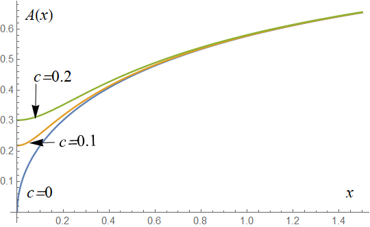
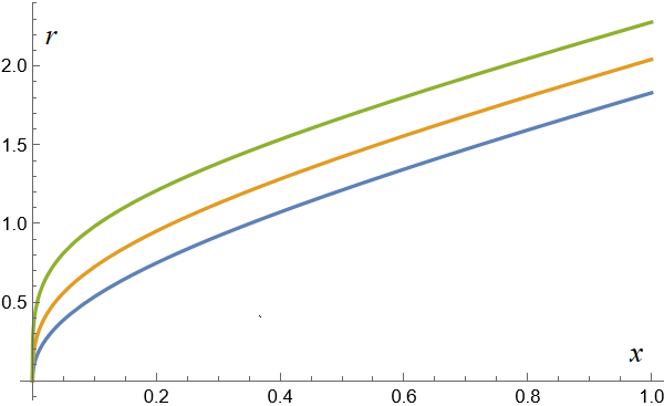
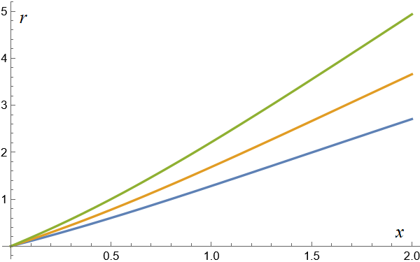
(a)                                              (b)                                              (c)

Figure 1: Fisher’s solution and its regularization. (a) The function $A(x)$ for Fisher’s solution ($c=0$) with $k=1,a=1/2$, and its regularized version with two values of $c$. (b) The spherical radius $r(x)$ in Fisher’s solution with $k=1$ and $a=0.1,0.3,0.5$ (bottom-up). (c) The spherical radius $r(x)$ in regularized Fisher’s solution with $k=1$, $c=0.2$, and $a=0.1,0.3,0.5$ (bottom-up).

Now, if we try to find a possible source for this metric with the action (8), it turns out that any of the two ways described in Sec. 2, either with Eq. (15) or with Eq. (20), leads to very complex integrals that evidently cannot be calculated analytically. For example, the expression of ${\mathcal{L}}^{\prime}(x)=d{\mathcal{L}}({\mathcal{F}}(x))/dx$ obtained from Eq. (20) reads (notations: $u=\sqrt{x^{2}+c^{2}},\ c_{1}=c^{2a/(1+a)},\ c_{2}=(c+2k)^{2/(1+a)}$)

$${}\frac{d{\mathcal{L}}(x)}{dx}=\frac{c^{a}(2k+u)^{-a-2}}{x^{3}u\left(c_{1}x^{2}+c_{2}\right)^{(1-a)/2}(c+2k)}\Big{(}2c_{1}x^{4}+[(1-a)c_{1}(c^{2}+2ku)+c_{2}(3+a)]x^{2}+2c_{2}(2ku+c^{2})\Big{)}$$

$${}\times\Bigg{(}\frac{c^{-a}u^{a}}{(c_{1}x^{2}+c_{2})^{(1+a)/2}(c+2k)}\bigg{[}\frac{(a+1)(a+3)x^{4}c_{1}^{2}(2k+u)}{\left(c_{1}x^{2}+c_{2}\right)^{2}}-\frac{5(a+1)c_{1}x^{2}(2k+u)}{c_{1}x^{2}+c_{2}}$$

$${}-\frac{2(a+1)^{2}c_{1}x^{4}}{u\left(c_{1}x^{2}+c_{2}\right)}+\frac{a(a+1)x^{4}}{u^{2}(2k+u)}-\frac{(a+1)x^{4}}{u^{3}}+\frac{5(a+1)x^{2}}{u}+2(2k+u)\bigg{]}$$

$${}-\frac{2akx^{2}c^{-a}u^{a-5}\left[2(a-1)kux^{2}+c^{4}-c^{2}\left(x^{2}-2ku\right)-2x^{4}\right]}{(2k+u)(c_{1}x^{2}+c_{2})^{(1+a)/2}(c+2k)}-2(c+2k)\Bigg{)}.$$ (37)

However, the behavior of the function ${\mathcal{L}}({\mathcal{F}})$ turns out to be rather simple, as illustrated by the plots of ${\mathcal{L}}(x)$ in Fig. 2(a) and for ${\mathcal{L}}({\mathcal{F}})$ in Fig. 2(b). As was expected, there is a logarithmic divergence as $r_{\rm reg}(x)\to 0$ (${\mathcal{F}}\to\infty$) and a sufficiently rapid decay as $r_{\rm reg}(x)\to\infty$ (${\mathcal{F}}\to 0$), without a correct Maxwell limit at small ${\mathcal{F}}$ which would require ${\mathcal{L}}\approx{\mathcal{F}}$.

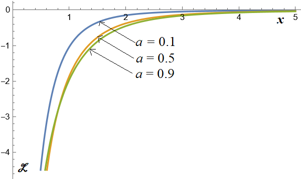
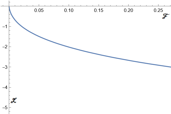
(a)                                              (b)

Figure 2: A possible source for the regularized Fisher solution: (a) The function ${\mathcal{L}}(x)$ for $k=1,\ c=0.2$, and $a=0.1,0.5,0.9$. (b) The function ${\mathcal{L}}({\mathcal{F}})$ for $k=1,\ c=0.2,\ a=0.5$, and $q=1$ (so that ${\mathcal{F}}=2/r_{\rm reg}^{4}$).

The scalar source $\phi$ of the regularized solution (not to be confused with $\Phi$ from the original singular solution) is characterized by the potential $V(\phi(x))$ and the function $h(\phi(x))$ whose sign is of particular interest for us since it determines the canonical or phantom nature of the source, whereas the function $\phi(x)$ may be chosen arbitrarily, it should only be monotonic. Assuming for convenience

$$\phi=\arctan{x/c},$$ (38)

with the functions $A=A_{\rm reg}(x)$ and $r=r_{\rm reg}(x)$ according to (35) and (4.1), we find from Eq. (19)

$${}h(\phi(x))=-\frac{r^{\prime\prime}}{r}\frac{(x^{2}+c^{2})^{2}}{c^{2}}=-\frac{(1+a)u}{4c^{2}(2k+u)^{2}[(c+2k)^{2/(1+a)}+c^{2a/(1+a)}x^{2}]^{2}}$$

$${}\times\Big{[}6c^{2}(c+2k)^{4/(1+a)}(2k+u)-6c^{4+2a/(1+a)}(c+2k)^{2/(1+a)}(4k+u)-(1-a)c^{4+4a/(1+a)}(4k+u)x^{2}$$

$${}+(c+2k)^{4/(1+a)}[8k+(3+a)u]x^{2}-4(1-a)c^{4a/(1+a)}k^{2}ux^{4}$$

$${}-2c^{2a/(1+a)}(c+2k)^{2/(1+a)}x^{2}\{12k^{2}u(1+c^{2})+2x^{2}[(3+a)k+u]+c^{2}x^{2}[2(7+a)k+(1+a)u]\}$$

$${}+2c^{2+4a/(1+a)}x^{2}[u(-2k^{2}+x^{2})+2ak(ku+x^{2})]\Big{]},$$ (39)

where, as before, $u=\sqrt{x^{2}+c^{2}}$. As can be seen from Fig. 3(a), we have obtained $h<0$ at small values of $x$, near the new regular center. At larger $x$, the scalar is canonical, and thus we are dealing with what has been called a trapped ghost scalar, showing a phantom nature only in a strong field region [56]. It can also be noticed for the curves in Fig. 1(b) that $r^{\prime\prime}<0$, corresponding to $h>0$, while Fig. 1(c) shows curves with small positive $r^{\prime\prime}$ (at least cllose to $x=0$), corresponding to $h<0$. The behavior of the potential $V(\phi(x))$, determined using Eq. (21), is shown in Fig. 3(b); its $\phi$ dependence is easily reproduced according to (38) by substituting $x=c\tan\phi$.

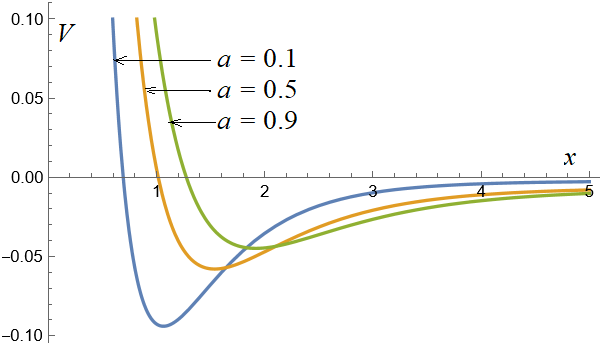
(a)                                              (b)

Figure 3: A possible source for the regularized Fisher solution: (a) The function $h(\phi(x))$ at $k=1,\ c=0.1$, and different values of $a$. The plane $h=0$ is drawn to visualize the region with $h<0$. (b) The function $V(\phi(x))$ for $k=1,\ c=0.2,\ a=0.1,0.5,0.9$.

4.2 A dilatonic black hole

Dilatonic black holes are described by special solutions of GR with a source consisting of a massless scalar field $\Phi$ interacting with an electromagnetic field according to the action

$$S_{\rm dil}=\dfrac{1}{2}\int\sqrt{-g}\,d^{4}x\big{[}2g^{\mu\nu}\Phi_{,\mu}\Phi_{,\nu}-{\,\rm e}^{2\lambda\Phi}F_{\mu\nu}F^{\mu\nu}\big{]},$$ (40)

where $\lambda$ is a coupling constant. The corresponding black hole solution can be written in terms of the metric (3) with [47, 48, 49, 50]

$$A(x)=\Big{(}1-\frac{2k}{x}\Big{)}\Big{(}1+\frac{p}{x}\Big{)}^{-2/(1+\lambda^{2})},\qquad r^{2}(x)=x^{2}\Big{(}1+\frac{p}{x}\Big{)}^{2/(1+\lambda^{2})},$$ (41)

while the scalar $\Phi$ and the electric field $\vec{E}$ are given by

$$\Phi=-\frac{\lambda}{1+\lambda^{2}}\ln\Big{(}1+\frac{p}{x}\Big{)},\qquad 2{\vec{E}}{}^{2}=-F_{\mu\nu}F^{\mu\nu}=\frac{Q^{2}}{r^{4}(x)}{\,\rm e}^{-4\lambda\Phi},$$ (42)

where $Q$ is the electric charge, $k$ is one more integration constant, and $p=\sqrt{k^{2}+Q^{2}(1+\lambda^{2})}-k>0$.

Consider the case $\lambda=1$ related to string theory dil2, dil3. Then the metric has the simple form

$$ds^{2}=\frac{1-2k/x}{1+p/x}dt^{2}-\frac{1+p/x}{1-2k/x}dx^{2}-x(x+p)d\Omega^{2}.$$ (43)

with a horizon at $x=2k$, a singularity at $x=0$, and the Schwarzschild mass $m=k+p/2=Q^{2}/p$.

The singularity $x=0$ is located beyond the horizon, and since there $A\to-2k/p={\rm const}$, it seems to be the relatively complex case, however, fortunately, due to the simple structure of $A(x)$, it is readily regularized by the substitution (27) with $m=1$. Taking there $n=1$, we obtain

$$A_{\rm reg}(x)=\frac{(x^{2}+c^{2})^{3/2}-2kx^{2}}{(x^{2}+c^{2})^{3/2}+px^{2}}.$$ (44)

For Step 2 we have $r_{1}(x)=\sqrt{x+p}$, consequently,

$${}a=0,\qquad b=1/2,\qquad N=-1/4,\qquad\alpha=1/(c+p)^{2},$$

$${}r_{\rm reg}^{2}(x)=\frac{x^{2}\big{(}\sqrt{x^{2}+c^{2}}+p\big{)}}{\sqrt{x^{2}+(c+p)^{2}}},$$ (45)

and we can write the regularized metric in the form (34) with $A_{\rm reg}$ and $r_{\rm reg}$ given by (44) and (4.2). The smoothed form $A_{\rm reg}$ of $A(x)$ is shown in Fig. 4 for particular values of the parameters. As to the radius (4.2), its $x$ dependence is very close to $r_{\rm reg}\approx x$ and weakly depends on the parameters $p$ and $c$, so it does not make sense to show its plots.

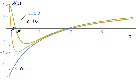
Figure 4: The dilatonic black hole solution (43) and its regulrization. The function $A(x)$ for with $k=p=1$ ($c=0$) and its regularized versions with two nonzero values of $c$.

As in the previous subsection, let us use Eq. (20) to obtain an expression for $d{\mathcal{L}}/dx$ for a possible NED source of the regularized metric (as before, $u=\sqrt{x^{2}+c^{2}}$):

$${}\frac{d{\mathcal{L}}}{dx}=-\frac{2\Big{[}(x^{2}/u)\left((c+p)^{2}+x^{2}\right)+(p+u)\left(2(c+p)^{2}+x^{2}\right)\Big{]}}{x^{3}(p+u)^{2}{u^{3}\left((c+p)^{2}+x^{2}\right)^{3}\left(px^{2}+u^{3}\right)}}$$

$${}\times\bigg{\{}-\left(u^{3}-2kx^{2}\right)\Big{[}-2u^{3}(c+p)^{4}(p+u)+u^{2}x^{2}(c+p)^{2}\Big{(}u(p+u)\left((c+p)^{2}+1\right)-5(c+p)^{2}\Big{)}$$

$${}+x^{6}\left(2(c+p)^{2}+pu^{3}+u^{4}-3u^{2}\right)+x^{4}(c+p)^{2}\left((c+p)^{2}+2pu^{3}+2u^{4}-8u^{2}\right)+x^{8}\Big{]}$$

$${}-2{u^{3}\left((c+p)^{2}+x^{2}\right)^{5/2}\left(px^{2}+u^{3}\right)}\bigg{\}}.$$ (46)

Unlike the case with Fisher’s solution, it is now possible to integrate this expression analytically, but the result is too cumbersome to handle. Instead, in Fig. 5 we present examples of ${\mathcal{L}}(x)$ and ${\mathcal{L}}({\mathcal{F}})$ for some values of the parameters, obtained by numerical integration. It is observed, in particular, that in this case the NED Lagrangian exhibits a Maxwell-like behavior at small ${\mathcal{F}}$.

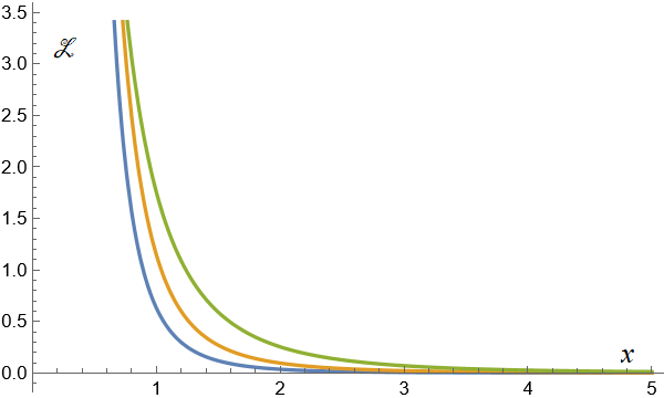
(a)                                              (b)

Figure 5: A possible source of the regularized solution for a dilatonic black hole: (a) The function ${\mathcal{L}}({\mathcal{F}}(x))$ for $k=1,c=0.2$, and $p=0.1,\ 1,\ 5$ (bottiom-up). (b) The function ${\mathcal{L}}({\mathcal{F}})$ for the same parameter values.

The function $h(\phi(x))$ is, as before, easily calculated from Eq. (19), where we again choose $\phi=\arctan{x/c}$. Then, with the functions $A=A_{\rm reg}(x)$ and $r=r_{\rm reg}(x)$ given by (44) and (4.2), we obtain

$${}h(\phi(x))=-\frac{r^{\prime\prime}}{r}\frac{(x^{2}+c^{2})^{2}}{c^{2}}=-\frac{pu}{4c^{2}(p+u)^{2}(c^{2}+2cp+p^{2}+x^{2})^{2}}\Big{\{}-6c^{6}+12c^{5}u$$

$${}\qquad+12c^{4}(2p^{2}+2pu-x^{2})+px^{2}(4p^{3}-3p^{2}u-6px^{2}-3ux^{2})+4c^{3}(6p^{3}+3p^{2}u-3px^{2}+2ux^{2})$$

$${}\qquad+c^{2}(6p^{4}+10p^{2}x^{2}+9pux^{2}-6x^{4})+4c(4p^{3}x^{2}-3px^{4}-ux^{4})\Big{\}}$$ (47)

where $u=\sqrt{x^{2}+c^{2}}$. As was the case with Fisher’s metric, it happens that the sign of $h(\phi)$ changes from negative to positive at growing $x$, indicating a phantom nature of the scalar field $\phi$ in a strong field region near the center and its canonical nature elsewhere, see Fig. 6(a).

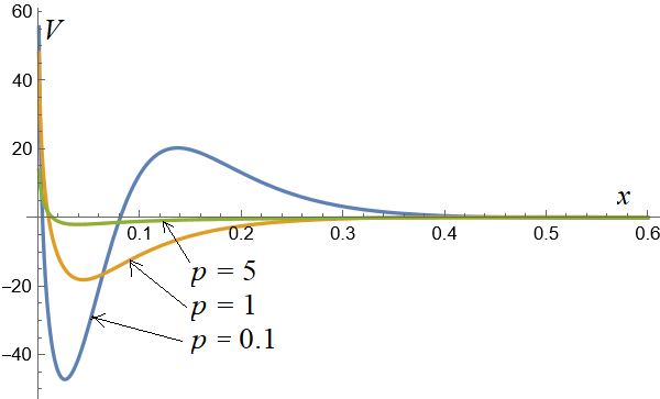
(a)                                              (b)

Figure 6: A possible source of the regularized solution for a dilatonic black hole: (a) The function $h(\phi(x))$ at $k=1,\ c=0.1$, and different values of $p$. Its behavior is qualitatively similar to Fig. 3(a). (b) The function $V(\phi(x))$ for $k=1,\ c=0.2,\ p=0.1,1,5$.

The scalar field potential $V(\phi(x)$, determined using Eq. (21), is shown in Fig. 6(b); as before, its $\phi$ dependence is easily found by substituting $x=c\tan\phi$.

5 Concluding remarks

1. In the present paper, extending the study begun in [45], we discuss the ways of singularity removal applicable to some kinds of static, spherically symmetric space-times, by properly changing a neighborhood of a singularity at $r=0$ so that it becomes a regular center. It is each time achieved by introducing a small regularization parameter, but quite different algorithms are required when dealing with different kinds of singularities. Thus, in all cases where the original singular space-time satisfying the condition $R^{t}_{t}=R^{x}_{x}$, the Bardeen-like regularization proposed in [45] preserves this condition, and the resulting space-time can be presented as a magnetic solution of Einstein-NED equations, similarly to papers describing regular black holes with a NED source (see [60, 65] and references therein).

2. More involved are cases where the above condition is not fulfilled, and here we considered singularities described by powers of the quasiglobal coordinate $x$ that does not coincide with the spherical radius $r$. The simplest examples of such space-times are given by Fisher’s solution for a massless minimally coupled scalar field in GR and some known dilatonic black hole solutions, which are here subject to singularity removal. Quite evidently, the metrics that are better represented with other coordinates, can be regularized by other (but similar) algorithms. On the other hand, even if it is hard to transform a particular metric to the quasiglobal coordinate $x$, quite probably such a transition can be carried out approximately near the singularity, and then the algorithms described here will be applicable.

3. It has been previously shown [20] that any static, spherically symmetric metric may be described as a solution of GR with a combined source consisting of a magnetic field obeying NED and a scalar field with a certain self-interaction potential. It, however, turned out that such a description of the presently regularized Fisher and dilatonic black hole solution leads to integrals that cannot be found analytically, whereas the same problem for their black-bounce regularizations was solved much easier [20], although the global structure of space-time is more complicated in the latter case.

4. All black-bounce space-times contain regular minima of the spherical radius $r$ and thus inevitably require phantom matter as a source if considered as solutions of GR. Obtaining regular centers instead of singularities does not necessarily require such exotic matter, though does not always avoid it. Thus, the examples considered in [45] with $R^{t}_{t}=R^{r}_{r}$ did not require any exotic matter; unlike that, in the presently considered examples of regularized Fisher and dilatonic black hole metrics it turned out that such exotic matter is needed near the center, as shown in Figs. 3(a) and 6(a).

One can further study various features of the new regular metrics obtained here as well as those resulting from other similar regularizations, in particular, their geodesic structures, gravitational lensing, quasinormal modes, stability, thermodynamic properties, etc. In particular, the stability properties of these metrics may crucially depend on the dynamics of their sources of gravity. Thus, for example, it is known that the stability of the Ellis wormhole geometry [66, 67] depends on whether its source is a phantom scalar field, a perfect fluid or a k-essence field [68, 69, 70]. On the other hand, Fisher’s solution (4.1) was found to be unstable due to its behavior near its naked singularity [71], and it would be of interest to know, how its different regularizations (the black-bounce one [20] and the one described here) and their associated sources affect its stability.

Funding

We acknowledge the support from RUDN Project no. FSSF-2023-0003.

References

- [1] D. Malafarina, Classical collapse to black holes and quantum bounces: A review, Universe 3, 48 (2017).
- [2] H. M. Haggard and C. Rovelli, Black hole fireworks: quantum-gravity effects outside the horizon, spark black to white hole tunneling. Phys. Rev. D 92, 104020 (2015).
- [3] L. Modesto, Space-time structure of loop quantum black hole. Int. J. Theor. Phys. 49, 1649 (2010).
- [4] J. G. Kelly, R. Santacruz, and E. Wilson-Ewing, Black hole collapse and bounce in effective loop quantum gravity, arXiv: 2006.09325.
- [5] J.B. Achour, S. Brahma, S. Mukohyama, and J.-P. Uzan, Towards consistent black-to-white hole bounces from matter collapse, JCAP 2020, 20 (2020).
- [6] R.G. Daghigh, M.D. Green, J.C. Morey, and G. Kunstatter, Perturbations of a single-horizon regular black hole, arXiv: 2009.02367.
- [7] A. Ashtekar and J. Olmedo, Properties of a recent quantum extension of the Kruskal geometry, arXiv: 2005.02309.
- [8] C. Bambi, D. Malafarina, and L. Modesto, Non-singular quantum-inspired gravitational collapse. Phys. Rev. D 88, 044009 (2013).
- [9] Douglas M. Gingrich, Quasinormal modes of a nonsingular spherically symmetric black hole effective model with holonomy corrections, arXiv: 2404.04447.
- [10] Alexey S. Koshelev and Anna Tokareva, Non-perturbative quantum gravity denounces singular black holes, arXiv: 2404.07925.
- [11] Pablo Bueno, Pablo A. Cano, Robie A. Hennigar Regular black holes from pure gravity, arXiv: 2403.04827.
- [12] J.M. Bardeen, Non-singular general-relativistic gravitational collapse, in: Proc. Int. Conf. GR5 (Tbilisi, USSR, 1968), p. 174.
- [13] S.A. Hayward, Formation and evaporation of nonsingular black holes. Phys. Rev. Lett. 96, 031103 (2006); arXiv: gr-qc/0506126.
- [14] Regular Black Holes: Towards a New Paradigm of Gravitational Collapse, (Ed. Cosimo Bambi, Springer, Singapore, 2023). Preface and contents: arXiv: 2307.13249.
- [15] Chen Lan, Hao Yang, Yang Guo, Yan-Gang Miao, Regular black holes: A short topic review. Int. J. Theor. Phys. 62, 202 (2023); arXiv: 2303.11696.
- [16] Lorenzo Sebastiani and Sergio Zerbini, Some remarks on non-singular spherically symmetric space-times, arXiv: 2206.03814.
- [17] A. Simpson and M. Visser, Black bounce to traversable wormhole, JCAP 02, 042 (2019).
- [18] E. Franzin, S. Liberati, J. Mazza, A. Simpson and M. Visser, Charged black-bounce spacetimes, JCAP 07, 036 (2021).
- [19] F. S. N. Lobo, M. E. Rodrigues, M. V .d.S. Silva, A. Simpson, and M. Visser, Novel black-bounce spacetimes: wormholes, regularity, energy conditions, and causal structure, Phys. Rev. D 103, 084052 (2021).
- [20] K.A. Bronnikov, On black bounces, wormholes and partly phantom scalar fields. Phys. Rev. D 106, 064029 (2022); arXiv: 2206.09227.
- [21] J. Mazza, E. Franzin and S. Liberati, A novel family of rotating black hole mimickers, JCAP 04, 082 (2021).
- [22] Z. Xu and M. Tang, Rotating spacetime: black-bounces and quantum deformed black hole, Eur. Phys. J. C 81, 863 (2021).
- [23] R. Shaikh, K. Pal, K. Pal and T. Sarkar, Constraining alternatives to the Kerr black hole, Mon. Not. Roy. Astron. Soc. 506, 1229 (2021).
- [24] Y. Yang, D. Liu, Z. Xu, Y. Xing, S. Wu and Z. W. Long, Echoes of novel black-bounce spacetimes, Phys. Rev. D 104, 104021 (2021).
- [25] M. S. Churilova and Z. Stuchlik, Ringing of the regular black-hole/wormhole transition, Class. Quant. Grav. 37, 075014 (2020).
- [26] M. Guerrero, G. J. Olmo, D. Rubiera-Garcia and D. S. C. Gómez, Shadows and optical appearance of black bounces illuminated by a thin accretion disk, JCAP 08, 036 (2021).
- [27] N. Tsukamoto, Gravitational lensing by two photon spheres in a black-bounce spacetime in strong deflection limits, Phys. Rev. D 104, 064022 (2021).
- [28] S. U. Islam, J. Kumar and S. G. Ghosh, Strong gravitational lensing by rotating Simpson-Visser black holes, JCAP 10, 013 (2021).
- [29] X. T. Cheng and Y. Xie, Probing a black-bounce, traversable wormhole with weak deflection gravitational lensing, Phys. Rev. D 103, 064040 (2021).
- [30] K. A. Bronnikov and R. A. Konoplya, Echoes in brane worlds: Ringing at a black hole-wormhole transition, Phys. Rev. D 101 064004 (2020); arXiv: 1912.05315.
- [31] N. Tsukamoto, Gravitational lensing in the Simpson-Visser black-bounce spacetime in a strong deflection limit, Phys. Rev. D 103, 024033 (2021).
- [32] Haroldo C. D. Lima Junior, Luis C. B. Crispino, Pedro V. P. Cunha, and Carlos A. R. Herdeiro, Can different black holes cast the same shadow? Phys. Rev. D 103, 084040 (2021); arXiv: 2102.07034.
- [33] J. R. Nascimento, A. Y. Petrov, P. J. Porfirio and A. R. Soares, Gravitational lensing in black-bounce spacetimes, Phys. Rev. D 102, 044021 (2021).
- [34] Edgardo Franzin, Stefano Liberati, Jacopo Mazza, Ramit Dey, and Sumanta Chakraborty, Scalar perturbations around rotating regular black holes and wormholes: quasi-normal modes, ergoregion instability and superradiance, Phys. Rev. D 105, 124051 (2022); arXiv: 2201.01650.
- [35] Sunny Vagnozzi et al., Horizon-scale tests of gravity theories and fundamental physics from the Event Horizon Telescope image of Sagittarius A, Class. Quantum Grav. 40, 165007 (2023); arXiv: 2205.07787.
- [36] Davide Pedrotti, Sunny Vagnozzi See the lightning, hear the thunder: quasinormal modes-shadow correspondence for rotating regular black holes, arXiv: 2404.07589.
- [37] Saptaswa Ghosh, Arpan Bhattacharyya, Analytical study of gravitational lensing in Kerr-Newman black-bounce spacetime, JCAP 11, 006 (2022); arXiv: 2206.09954.
- [38] Abhishek Chowdhuri, Saptaswa Ghosh, Arpan Bhattacharyya, A review on analytical studies in gravitational lensing, Front. Phys. 11, 1113909 (2023); arXiv: 2303.02069.
- [39] K. A. Bronnikov and J. C. Fabris, Regular phantom black holes, Phys. Rev. Lett. 96, 251101 (2006).
- [40] K. A. Bronnikov, V. N. Melnikov and H. Dehnen, Regular black holes and black universes, Gen. Rel. Grav. 39, 973 (2007).
- [41] S. V. Bolokhov, K. A. Bronnikov and M. V. Skvortsova, Magnetic black universes and wormholes with a phantom scalar, Class. Quantum Gravity 29, 245006 (2012).
- [42] G. Clement, J. C. Fabris and M. E. Rodrigues, Phantom black holes in Einstein-Maxwell-dilaton theory, Phys. Rev. D 79, 064021 (2009).
- [43] M. Azreg-Ainou, G. Clement, J. C. Fabris and M. E. Rodrigues, Phantom black holes and sigma models, Phys. Rev. D 83, 124001 (2011).
- [44] K. A. Bronnikov. Scalar fields as sources for wormholes and regular black holes, Particles 2018, 1, 5; arXiv: 1802.00098.
- [45] K.A. Bronnikov, Regular black holes as an alternative to black bounce, arXiv: 2404.14816.
- [46] I. Z. Fisher, Scalar mesostatic field with regard for gravitational effects, J. Eksp. Teor. Fiz. 18, 636 (1948); gr-qc/9911008 (translation into English).
- [47] K. A. Bronnikov and G. N. Shikin, On interacting fields in general relativity, Russ. Phys. J. 20, 1138–1143 (1977).
- [48] G. W. Gibbons and K.-i. Maeda, Black holes and membranes in higher dimensional theories with dilaton fields, Nucl. Phys. B 298, 741 (1988).
- [49] D. Garfinkle, G.T. Horowitz, and A. Strominger, Charged black holes in string theory, Phys. Rev. D 43, 3140 (1991). [Erratum: Phys. Rev. D 45, 3888 (1992)].
- [50] K.A. Bronnikov. Spherically symmetric solutions in D-dimensional dilaton gravity, Grav. Cosmol. 1, 67 (1995).
- [51] K. A. Bronnikov and R. K. Walia, Field sources for Simpson-Visser space-times, Phys. Rev. D 105, 044039 (2022); arXiv: 2112.13198.
- [52] Pedro Cañate, Black-bounces as magnetically charged phantom regular black holes in Einstein-nonlinear electrodynamics gravity coupled to a self-interacting scalar field, Phys. Rev. D 106, 024031 (2022); arXiv: 2202.02303.
- [53] Leonardo Chataignier, Alexander Yu. Kamenshchik, Alessandro Tronconi, and Giovanni Venturi, Regular black holes, universes without singularities, and phantom-scalar field transitions, Phys. Rev. D 107, 023508 (2023); arXiv: 2208.02280.
- [54] Alexander Kamenshchik and Polina Petriakova, Regular Friedmann universes and matter transformations, Universe 10 (3), 137 (2024); arXiv: 2403.08400.
- [55] H. Kroger, G. Melkonian and S. G. Rubin, Cosmological dynamics of scalar field with non-minimal kinetic term, Gen. Rel. Grav. 36, 1649 (2004).
- [56] K. A. Bronnikov and S. V. Sushkov, Trapped ghosts: a new class of wormholes, Class. Quantum Grav. 27, 095022 (2010).
- [57] K. A. Bronnikov and E. V. Donskoy, Black universes with trapped ghosts. Grav. Cosmol. 17 (1), 31 (2011); arXiv: 1110.6030.
- [58] K. A. Bronnikov. Trapped ghosts as sources for wormholes and regular black holes. The stability problem. In: Wormholes, Warp Drives and Energy Conditions, ed. F.S.N. Lobo, Springer, 2017, p. 137-160.
- [59] K. A. Bronnikov and S. G. Rubin. Black Holes, Cosmology, and Extra Dimensions (2nd edition, World Scientific, 2021).
- [60] K.A. Bronnikov, Regular magnetic black holes and monopoles from nonlinear electrodynamics, Phys. Rev. D 63, 044005 (2001).
- [61] K.A. Bronnikov, Comment on “Regular black holes in general relativity coupled to nonlinear electrodynamics,” Phys. Rev. Lett. 85, 4641 (2000).
- [62] G. Alencar, K.A. Bronnikov, M.E. Rodrigues, D. Sáez-Chillón Gómez, Marcos V.de S. Silva, On black bounce space-times in non-linear electrodynamics, arXiv: 2403.12897.
- [63] A. I. Janis, E. T. Newman, and J. Winicour, Reality of the Schwarzschild singularity, Phys. Rev. Lett. 20, 878 (1968).
- [64] Max Wyman, Static spherically symmetric scalar fields in general relativity, Phys. Rev. D 24, 839 (1981).
- [65] K.A. Bronnikov, Regular black holes sourced by nonlinear electrodynamics, in: “Regular Black Holes. Towards a New Paradigm of Gravitational Collapse,” (Ed. by Cosimo Bambi, Springer Series in Astrophysics and Cosmology (SSAC)) p. 37–67; arXiv: 2211.00743.
- [66] H. G. Ellis, Ether flow through a drainhole: a particle model in general relativity, J. Math. Phys. 14, 104 (1973).
- [67] K.A. Bronnikov, Scalar-tensor theory and scalar charge, Acta Phys. Pol. B 4, 251 (1973).
- [68] J.A. González, F.S. Guzmán and O. Sarbach, Instability of wormholes supported by a ghost scalar field. I. Linear stability analysis, Class. Quantum Grav. 26, 015010 (2009); arXiv: 0806.0608.
- [69] K. A. Bronnikov, L. N. Lipatova, I. D. Novikov, and A. A. Shatskiy, Example of a stable wormhole in general relativity. Grav. Cosmol. 19, 269 (2013).
- [70] Kirill A. Bronnikov, Vinicius A. G. Barcellos, Laura P. de Carvalho, and Júlio C. Fabris, The simplest wormhole in Rastall and k-essence theories. Eur. Phys. J. C 81, 395 (2021); arXiv: 2102.10797.
- [71] K.A. Bronnikov and A.V. Khodunov. Scalar field and gravitational instability, Gen. Rel. Grav. 11, 13 (1979).