Complex-valued 3D atomic spectroscopy with Gaussian-assisted inline holography

Abstract

When a laser-cooled atomic sample is optically excited, the envelope of coherent forward scattering can often be decomposed into a few complex Gaussian profiles. The convenience of Gaussian propagation helps addressing key challenges in digital holography. In this work, we theoretically develop and experimentally demonstrate a Gaussian-decomposition-assisted approach to inline holography, for single-shot, simultaneous measurements of absorption and phase shift of small atomic samples sparsely distributed in 3D. Experimentally, we image a sparse lattice of ⁸⁷Rb samples on the D2 line, to resolve their axial positions with micrometer precision, and to retrieve their complex-valued spectroscopic images. With the phase-angle readouts that are highly insensitive to atom-number and interaction-strength uncertainties, we achieve hundred-kHz-level single-shot-resolution to the transition frequency with merely hundreds of atoms. We further demonstrate 3D sensing of local light shift with micrometer spatial resolution.

I Introduction

Atoms are ideal quantum sensors. By measuring the optical response of free atoms, the centers and linewidths of atomic levels can be accurately inferred for unveiling unknown interactions and to calibrate external potentials [1, 2, 3, 4]. The optical transition properties are affected by the center-of-mass motion. The laser-cooling techniques, which are able to effectively freeze the atomic motion, was expected to greatly enhance the precision of atomic spectroscopy [5]. Nowadays, however, while laser cooling and trapping are often essential in spectroscopic measurements on narrow transitions [6, 7, 8, 9, 10], precision spectroscopy on strong transitions tends to rely more on traditional sources such as saturated vapors [11] and atomic beams [12]. Compared to the thermal sources, the fluxes from cold-atom sources are moderate and easily fluctuate. Furthermore, during a prolonged probe period, the light-atom interaction strength, characterized by the atomic polarizability $\alpha$, can be modified by optical pumping even at extremely low light levels [13]. Efficient suppression of the systematic errors associated with such fluctuations are important for atomic precision spectroscopy to fully benefit from the long-time Doppler-free interaction offered by laser cooling, and to enable novel applications of ultra-cold atoms such as for wideband quantum sensing of 3D potentials  [14, 15, 16].

The impacts of atom number and interaction-strength fluctuations can be substantially suppressed in atomic spectroscopy, if one is able to extend the spectroscopic data from real to complex numbers. In particular, for a dilute atomic sample subjected to a near-resonant probe [17], both the optical depth ${\rm OD}$ and phase shift $\phi$ are proportional to the atom number $N$ and the modulus of the atomic polarizability $|\alpha|$. But the phase angle $\beta={\rm arg}(\phi+i{\rm OD}/2)$ is largely decided by the atomic phase angle, ${\rm arg}(\alpha)$, highly insensitive to the $N|\alpha|$ fluctuations [18, 19]. Unfortunately, it is not possible to simultaneously measure ${\rm OD}$ and $\phi$ distributions without precisely knowing the complex $E_{r}^{\prime}$ and $E_{r}$, the transmitted probe wavefronts in presence and absence of the atomic sample respectively. In standard transmission imaging techniques where the light intensities are recorded only [17, 20], the optical phase information are completely lost. While single-mode coherent transmission spectroscopy [21, 22, 23, 24] is able to retrieve the $E_{r}$-mode-averaged ${\rm OD}$ and $\phi$, the single-mode readouts cannot support spatial resolution in general. Furthermore, since details of atomic distribution are disregarded, it becomes difficult to correct for any density-dependent shifts in the collective responses [25, 26, 27].

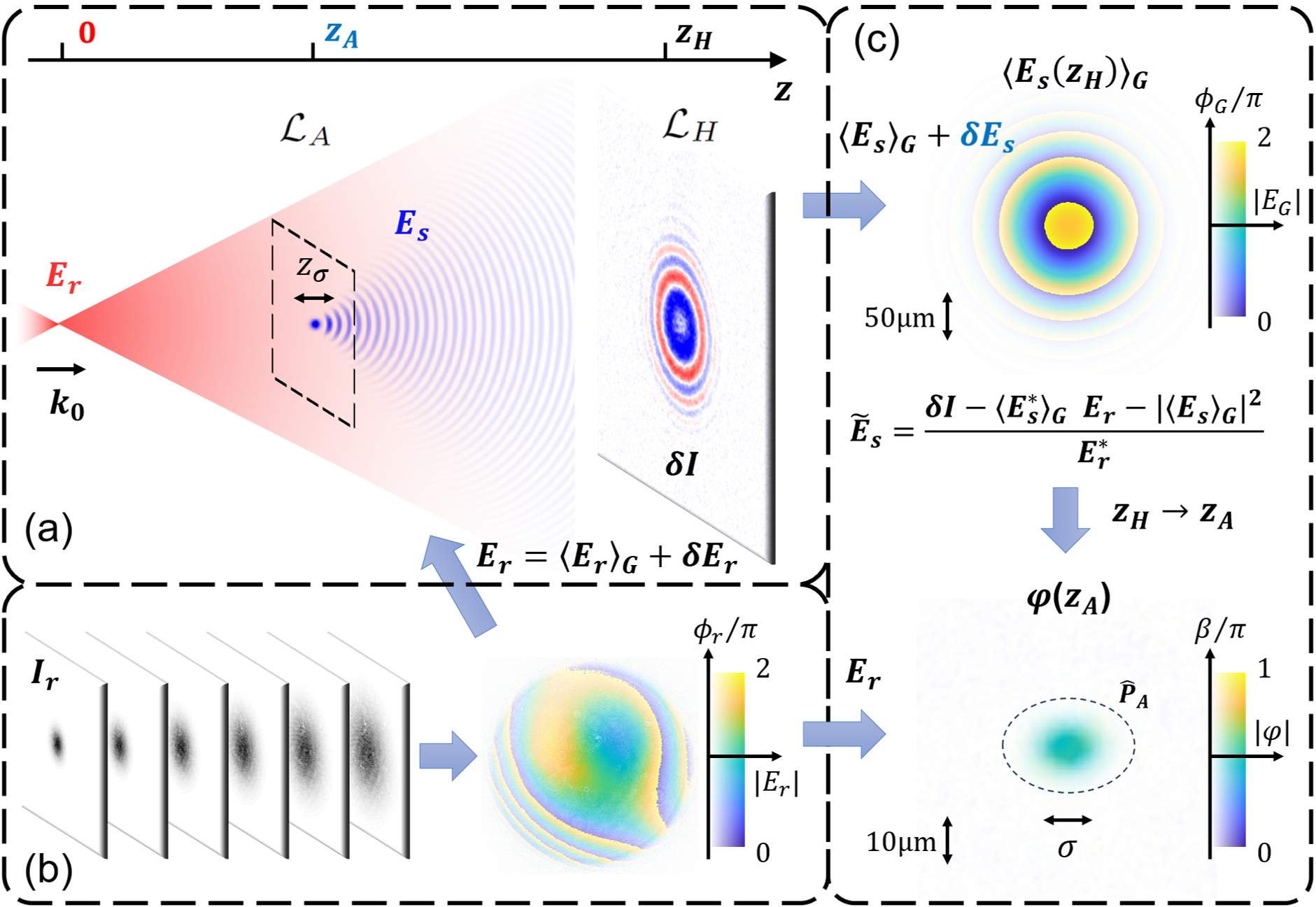
Figure 1: Complex spectroscopic imaging with Gaussian-decomposition-assisted inline holography. (a): The basic setup. (b): Pre-characterization of the reference field $E_{r}=\sqrt{I_{r}}e^{i\phi_{r}}$ through multi-plane intensity $I_{r}=|E_{r}|^{2}$ measurements [18]. The low-spatial-frequency part of the forward scattering $E_{s}=E_{r}^{\prime}-E_{r}$ is decomposed into multiple Gaussian profiles according to Eq. (7). The Gaussian propagation supports efficient minimization of $\mathcal{L}_{H}$ associated with the $\delta I=I^{\prime}-I$ data in the camera plane $z=z_{H}$, and $\mathcal{L}_{A}$ associated with the sample knowledge around $z=z_{A}$, according to Eq. (10). (c): The full $E_{s}$, approximated by $\tilde{E}_{s}$ in Eq. (13), is propagated together with $E_{r}$ to $z=z_{A}$ to retrieve the complex phase shift $\varphi(z_{A})$ as the complex-valued imaging data. The scale bars are according to typical experimental condition in this work. The (colored ) black symbols refer to quantities that are (not) precisely known at the represented stages of measurements.

In this work, we develop a systematic procedure for complex-valued spectroscopic imaging of laser-cooled atoms. The technique is based on inline holography [28, 29, 30, 18, 19]. To fix the optical phase ambiguity [31] by exploiting the prior knowledge about the atoms in a numerically efficient manner, we introduce a Gaussian-decomposition [32, 33, 34] method to digital holographic microscopy. For arrays of samples with known phase angle $\beta$, our method is able to retrieve the transmitted $E_{r}^{\prime}$ (and $E_{r}$) from single-shot hologram data while spectroscopically locating the centers of each sample in 3D with a super-resolution close to the photon-shot-noise limit (Cramer-Rao bound [35]). The absorption ${\rm OD}$ and phase-shift $\phi$ images can be numerically reconstructed to form the complex $\varphi_{A}=\phi+i{\rm OD}/2$ images, with diffraction-limited spatial resolution and photon-shot-noise limited sensitivity. Experimentally, we simultaneously reconstruct complex-valued spectroscopic images of sparsely distributed ⁸⁷Rb samples on the D2 line, from single-shot holograms which are recorded within tens of microseconds. By retrieving the phase angles, we demonstrate $100~{}$kHz-level resolution to the transition frequency and its shift using merely hundreds of atoms, with micrometer-level 3D spatial resolution, in presence of substantial shot-to-shot atom-number uncertainties.

In what follows, we first review the basic principles of the quantitative holographic imaging [36, 37, 38] for atomic spectroscopy [18]. We then introduce our new method where Gaussian decomposition [33, 34, 32] is applied into holography, to facilitate the phase retrieval and 3D localization of atomic samples.

I.1 Complex-valued imaging with inline holography

We consider the inline holography setup [31, 29] illustrated in Fig. 1a where a nearly spherical atomic sample at $z=z_{A}$, with a characteristic width $\sigma$, is resonantly excited by a spherical probe beam $E_{r}$ with optical frequency $\omega$, wavelength $\lambda$ and wavenumber $k_{0}=2\pi/\lambda$. The attenuation and phase shift to $E_{r}$ is encode in $E_{s}$, the coherent forward scattering from the sample. We therefore rewrite $E_{r}^{\prime}=E_{r}+E_{s}$. Defining [39]

$$\varphi(z)=-i{\rm log}(1+E_{s}(z)/E_{r}(z)),$$ (1)

then, according to Beer-Lambert law, we have the complex phase shift by the sample [18]

$$\varphi_{A}(x,y) =\varphi(x,y,z_{A}),$$ (2)

$$=\phi(x,y)+i{\rm OD}(x,y)/2,$$

$$\approx\frac{1}{2}k_{0}\rho_{c}(x,y)\alpha(\omega).$$

Here $\rho_{c}=\int\rho(z){\rm d}z$ is the column density. The $\alpha(\omega)$ is the atomic polarizability. The third line in Eq. (2) becomes accurate for small ensemble of dilute atoms with $k_{0}^{3}\rho\ll$1.

The transmitted $E_{r},E_{r}^{\prime}$ propagate further for a distance $z_{H}-z_{A}$ where the intensity is recorded by a digital camera. The intensities in presence and absence of the atomic sample are modeled as

$$I^{\prime} =\left|E_{r}(z_{H})+E_{s}(z_{H})\right|^{2},$$ (3)

$$I =\left|E_{r}(z_{H})\right|^{2},$$

respectively. The reduced hologram is defined as

$$\delta I=I^{\prime}-I.$$ (4)

Assuming the probe profile $E_{r}$ as known, the goal of holographic imaging is to infer through the $I^{\prime},I$ measurements the axial central location $z_{A}$ and to retrieve the 2D complex phase shift image $\varphi_{A}(x,y)$ (Eq. (2)) there.

I.2 Challenges

The quantitative holographic imaging technique [36, 37, 38] faces at least three categories of challenges, which are all amplified in cold atom setups [40, 41, 30, 42, 43, 18, 19]:

1. To retrieve $E_{s}$ from the $I^{\prime},I$ data with Eq. (3) is an ill-defined problem, requiring additional constraints to fix the $E_{s}$ solution not to be perturbed by its twin [31],

   $$E_{s,{\rm twin}}=\frac{E_{r}}{E_{r}^{*}}E_{s}^{*}$$ (5)

   at $z=z_{H}$, which focuses approximately at

   $$z_{\rm twin}=\frac{z_{A}z_{H}}{2z_{A}-z_{H}}.$$ (6)

   Due to the fragile nature of cold atomic samples and typical complexity of the setup that produce them, traditional solutions to the twin-image problem associated with phase-shifting [44] and multiple phase-diversity measurements [45, 46, 47] can not be easily implemented. While off-axes holography [48, 40, 42] is powerful for resolving the optical phase, the technique necessarily sacrifices some of the imaging bandwidth while adding more complexity to the setup. Finally, while structured illumination [49] may help solving the phase problem, the associated $E_{r}$ structure could complicate the light-atom interaction through Doppler shifts and transition saturation [13].

   Without resorting to additional measurements, the constraints available for cold atom holography typically only include those associated with finite spatial support [40, 30, 42, 18] and optical response characteristics [41, 43]. Previous applications of these prior knowledge, while leading to notable successes, may still not guarantee an accuracy for precision spectroscopy in presence of imaging noises.

2. The sample plane location $z_{A}$ is not known a prior for the numerical back-propagation of the reconstructed $E_{r},E_{s}$ [42, 19]. Retrieving ${\rm OD}$ and $\phi$ with the Eqs. (1)(2) relation in an out-of-focus plane mixes the absorption with phase shift [50, 51], leading to erroneous phase angle $\beta$.

   Cold atoms in a dilute enough gas typically follow a normal density distribution. The lack of distinct spatial features invalidates a class of traditional methods for sample-plane localization in digital holography [52, 53, 54, 55, 56]. While the sample plane can be precisely located by observing the atomic shot noise [43], the method is slow since many images are required for the statistical analysis.

3. While the $E_{r}$ wavefront is assumed known, any deviation of the actual $E_{r}$ induces distortion to the retrieved $E_{s}$, leading to erroneous $\varphi_{A}$. In particular, the speckle noises [57] in $E_{r}$ can hardly be avoided in atomic spectroscopy where the laser probe is necessarily monochromatic [30, 18].

I.3 This work

We develop a method for complex-valued spectroscopic imaging of sparsely distributed atomic samples in 3D. As outlined in Fig. 1, the method is based on inline holography [28]. The phase ambiguity associated with the twin image (Eq. (5)) is addressed by systematically exploiting our prior knowledge about the measurement. Apart from the hologram data (Eq. (3)), the pre-characterized $E_{r}$ wavefront [18], our prior knowledge is mostly about the bulk optical properties of the samples in focus, i.e., aspects of the complex phase shift profile $\varphi_{A}(x,y)$ at $z=z_{A}$. The key insight is that when the probe beam $E_{r}$ seen by the sample is locally smooth, then these properties can be efficiently parametrized by decomposing $E_{s}$ into a few Gaussian beams (see Eq. (36)) [32, 33, 34],

$$E_{G}({\bf r};\{c_{j},{\bf P}_{j}\})=\sum_{j=1}^{n_{A}}c_{j}G_{j}({\bf r};{\bf P}_{j}).$$ (7)

We denote the optimal decomposition as $\langle E_{s}\rangle_{G}=E_{G}({\bf r};\{c_{j},{\bf P}_{j}\}_{\rm opt})$. The Gaussian propagation facilitates simultaneous minimization of cost functions, $\mathcal{L}_{H}$ at $z=z_{H}$ (Eq. (11)) associated with the $I^{\prime},I$-data, and $\mathcal{L}_{A}$ at $z=z_{A}$ (Eq. (12)) associated with the expected $\varphi_{A}$.

Our method works especially well in a “defocused twin regime” (Appendix C.1) for small atomic samples, with $z_{\sigma}\ll z_{A},z_{H}-z_{A}$, so that there are sufficient interference fringes in the $I^{\prime}-$data (Eq. (4)). Here $z_{\sigma}=\pi\sigma^{2}/\lambda$ is the characteristic Rayleigh length of the sample. Key advantages of our method is summarized as follows:

1. Our method generalizes traditional single-shot twin-removal strategies such as those associated with finite spatial supports [58, 59, 30] and spectral phase angles [41, 60]. Here, bulk properties of the samples such as the approximate 3D locations, shapes, and spatial-(in)dependent spectral responses, can all be encoded into the $\varphi_{A}$-image-expectations to constrain the $\{c_{j},{\bf P}_{j}\}$ parameters. The enhanced application of prior knowledge improves the accuracy of the optical phase determination in presence of imaging noises.

2. With the phase angle $\beta={\rm arg}(\varphi_{A})$ constrained by knowledge of light-atom interaction [41, 43, 19], the atomic sample plane location $z_{A}$ can be conveniently inferred during Gaussian decomposition. For nearly spherical samples with $z_{\rm\sigma}\ll z_{A},z_{H}-z_{A}$, the typical axial resolution is [19] (Appendix A)

   $$\Delta z_{A}\approx z_{\sigma}/\sqrt{N_{s}},$$ (8)

   decided by the Rayleigh length $z_{\sigma}=\pi\sigma^{2}/\lambda$ associated with the sample size $\sigma$ (Fig. 1a). This resolution can be enhanced by introducing finer sample features, or simply by repeating the in situ measurements with standard samples to effectively increase the total number of coherently scattered photons $N_{s}=\sum_{x,y}|E_{s}|^{2}$ received by the camera.

3. With $z_{\sigma}\ll z_{A},z_{H}-z_{A}$, diffraction-limited $E_{r}$ and $E_{s}$ can be retrieved from single-shot $I^{\prime},I$ data, using the pre-characterized $E_{r}$ knowledge through multi-plane intensity measurements [18]. Impacts of mild speckle noises and moderate aberrations can be corrected, for achieving complex $\varphi_{A}(x,y)$ imaging with diffraction-limited resolution and photon-shot-noise limited sensitivity. The phase-angle resolution is given by [18] (Appendix A)

   $$\Delta\beta(\mathcal{A})\approx 1/\sqrt{2N_{s}(\mathcal{A})}.$$ (9)

   Here $N_{s}(\mathcal{A})=\sum_{\mathcal{A}}|E_{s}|^{2}$ integrates the elastically scattered photons over area $\mathcal{A}$ of interest in the in-focus $\varphi_{A}(x,y)$ image.

I.3.1 Application to atomic spectroscopic imaging

With the inclusion of both phase-angle $\beta$ and modulus $|\varphi_{A}|$ readouts into the spectroscopy data, the previously mentioned challenges in cold atom spectroscopy—stemming from fluctuations in atom number and interaction strength—become significantly more manageable. When combined with 3D imaging capabilities, our complex spectroscopy technique substantially improves the potential for imaging and sensing on strong optical transitions with laser-cooled atomic arrays.

It is important to note that compared to absorption [17] or phase contrast [20] techniques, holographic imaging incurs a 50$\%$ loss of information [40, 30] (see Appendix A). In the following, we argue that such a loss hardly disadvantages our single-shot complex spectroscopic approach in precision measurements.

To start with, our method avoids measurement noises associated with atom-number and interaction-strength normalization, which, except for special kind of samples with known atom number and fixed interaction strength [61], is typically required in precision spectroscopy [62]. To see the potential of holographic complex imaging at the fundamental level, we compare a special case of resonant absorption and holographic imaging, i.e., with the probe beam frequency $\omega$ tuned close to the transition frequency $\omega_{eg}$ so that the sample is absorptive. It is easy to show that compared to a double-shot absorption measurement, including one for atom-number and interaction-strength normalization (assuming as being performed perfectly), the holographic signals from two independent measurements support just the same, photon-shot-noise-limited absorption sensitivity.

Furthermore, the holographic measurement obtains the absorption and phase-shift image at the same time. The complex-valued spectroscopy is $\Delta$-sensitive at any detuning $\Delta=\omega-\omega_{eg}$. Near resonance, the absorption or fluorescence profiles are peaked and therefore lose the detuning-sensitivity to the first order. In contrast, on-resonance our complex spectroscopy achieves the best sensitivity, capable of resolving $\omega_{eg}$ within single shot through the phase-angle $\beta$ measurement. In the limit of low density [25] and/or high probe intensity [63], the phase angle $\beta$ is purely decided by the single-atom response [19], ideal for precision spectroscopy. Furthermore, with diffraction and shot-noise limited ${\rm OD}$, $\phi$ image data, minimal modeling of atomic distributions supports correction to density-dependent shifts [25].

Finally, it is worth noting that phase-angle spectroscopy can be substantially more robust against power broadening and optical pumping effects (Sec. II.4) [19] than those in regular spectroscopy. This, combined with the fact that the complex-valued spectroscopy does not require the sample to be nearly intact for the normalization later, suggesting that more efficient precision measurements are possible without requiring extremely low light-level operations [13, 62].

I.3.2 Major limitations in this work

Practically, our holographic imaging method [18] can be conveniently adapted to standard imaging setups, simply by translating the camera away from the atomic imaging plane for recording the inline interference patterns (Fig. 1a). Numerically, a key step is based on matching $E_{r},E_{s}$ with free-propagating Gaussian beams through the nonlinear minimization of Eq. (10). The method helps to overcome several major obstacles in quantitative holography, but also introduces substantial limitations. In the following we discuss major limitations and possible improvements.

First, the nonlinear optimization is quite slow. As we find in this work, while the analytical form of the Gaussian beam (Eq. (36)) [33, 34, 32] helps to avoid the resource-demanding, numerical propagation of full wavefronts [30, 18, 42, 43], to resolve single hologram still requires about 2 minutes even with a A100 GPU card (NVIDIA). Notably, for repeated measurements such as during a probe-frequency scan [1, 62], the processing time can be substantially reduced, down to tens of seconds, by seeding the optimization process with nearly optimal initial $\{c_{j},{\bf P}_{j}\}$-parameters. With more advanced software and hardware supports, we expect further improved imaging processing speed in future work.

Second, as detailed in Appendix C.1, diffraction-limited $\varphi(z_{A})-$image is most easily achieved for small samples satisfying $z_{\sigma}\ll z_{A},z_{H}-z_{A}$ (Fig. 1a) only. Beyond this “defocused-twin regime”, accurate $\varphi_{A}-$retrieval relies on improving the decomposition of $E_{s}$ using more Gaussian profiles (larger $n_{A}$), i.e., to capture fine details of $E_{s}$ so that the defocused twin-image noise (Eq. (13)) around $z=z_{A}$ is more efficiently removed. While the principle of such improvement as outlined in Sec. II.2 appears straightforward, its practicality in presence of imaging noise requires systematic study in future work. Nevertheless, we note that depending on the spatial resolution requirements, the $z_{A}$ and $z_{H}-z_{A}$ limited by the camera sensor size can typically be at a centimeter level. This in term supports sparse arrays with individual sample size of up to $100~{}\mu$m (Fig. 6), large enough for various applications. At moderate $z_{\sigma}$, the Gaussian-decomposition method can also be assisted by Gerchberg-Saxton-type iterations [58, 30, 29, 18] to improve the $E_{s}$ estimation.

Finally, the Gaussian-assisted holography method in this work assumes free-propagation between the sample plane at $z=z_{A}$ and camera plane at $z=z_{H}$. Practically, the atomic samples are often imaged to the camera plane through a lens array [17, 64, 43]. In this experimental work, the moderate, aplanatic aberrations in $E_{s}$ are corrected by a pre-characterized point-spread-function near the atomic sample location (Appendix D.3). Obviously, the method becomes insufficient in presence of strong astigmatism during, e.g., wide-field imaging [65, 66, 67]. In future work and with sufficient knowledge of the imaging system, full suppression of strong, astigmatic aberrations can be achieved by exploiting the Gaussian propagation across the lens array numerically [33, 34]. This may potentially enable diffraction-limited 3D complex-valued spectroscopic imaging across unprecedented imaging volumes, only limited by the pixel-size of the camera [68].

I.4 Structure of the rest of the paper

In the following the main text is structured into three sections. With technical details presented in Appendix B, we first outline the principles of the Gaussian-decomposition-assisted holographic imaging method in Sec. II. Next, in Sec. III we present experimental demonstration of diffraction and shot-noise limited complex-valued imaging. We summarize this work in Sec. IV.

II Principles

The schematic setup of our Gaussian-decomposition-assisted complex-valued spectroscopic imaging method is illustrated in Fig. 1(a-c). The Fig. 1a setup is already outlined in Sec. I.1. We regard the $(I^{\prime},I)$ measurement as a single-shot measurement. With in mind no atom-number or interaction-strength normalization measurement is required later, the $I^{\prime}$-exposure can be strong and elongated to substantially alter the atomic velocity and/or the internal atomic state population. The $I$-exposure is taken immediately after the atomic sample is dispersed from the $E_{r}$ illumination.

We assume the holographic imaging setup to be effectively lensless [30] so that the accurate propagation of wavefronts between $z_{A}$ and $z_{H}$ is modeled by Eq. (47), $E(z^{\prime})=\hat{U}(z^{\prime}-z)E(z)$, through angular spectrum method numerically. On the other hand, for repetitive short-distance propagation during numerical optimization, the Gaussian-decomposed $E_{r},E_{s}$ wavefronts are sampled according to the analytical Eq. (36) under paraxial approximation (also see Appendix D.3.).

The reconstruction of $\varphi_{A}(x,y)$ at $z=z_{A}$ is divided into Sec. II.1,II.2,II.3 steps.

II.1 Obtaining $E_{r}$

A prerequisite to recover $E_{s}$ through the holographic measurement with Eq. (3) is to characterize the $E_{r}$ wavefront precisely. The steps for the $E_{r}$ measurements are illustrated in Fig. 1(a,b), detailed in ref. [18]. Briefly, using the single-shot $I$-data, the probe wavefront $E_{r}=\sqrt{I}e^{i\phi_{r}}$ is obtained by intensity-matching $I$ to $I_{0}=|E_{r}^{(0)}(z_{H})|^{2}$. Here $\phi_{r}={\rm arg}(E_{r}^{(0)})$. $E_{r}^{(0)}$ is the pre-characterized probe wavefront, obtained with multi-plane intensity measurements of $E_{r}$, followed by Gerchberg-Saxton iteration [69] (Fig. 1b). Notice the $E_{r}$ wavefront measurement is designed to share the same optical path with the holographic measurement.

II.2 Minimal Gaussian-decomposition of $E_{s}$

We parametrize $E_{s}$ with $n_{A}$ Gaussian beams according to Eq. (7), and minimize the cost function

$$\mathcal{L}_{\rm tot}(z_{A},\{c_{j},{\bf P}_{j}\})=\mathcal{L}_{H}+\mathcal{L}_{A},$$ (10)

with

$$\mathcal{L}_{H}(\{c_{j},{\bf P}_{j}\})=\sum_{x,y}\left|\delta I-E_{r}^{*}E_{G}-E_{r}E_{G}^{*}-|E_{G}|^{2}\right|^{2},$$ (11)

and

$$\mathcal{L}_{A}(z_{A},\{c_{j},{\bf P}_{j}\})=\sum_{\mu}m_{\mu}C_{\mu}\left(\varphi_{G}(z_{A},\{c_{j},{\bf P}_{j}\})\right).$$ (12)

Here $\mathcal{L}_{A}$ is formulated into a list of $C_{\mu}$-constraints (Appendix B.2) weighted by $m_{\mu}$, which can be adjusted during the optimization. The $\varphi_{G}(z_{A};\{c_{j},{\bf P}_{j}\})=-i{\rm log}\left(1+E_{G}/\langle E_{r}\rangle_{G}\right)_{z=z_{A}}$ evaluates the complex-valued phase shift by Eq. (1), with $E_{r}$ replaced by the known Gaussian envelope $E_{r}\approx\langle E_{r}\rangle_{G}$. Simultaneous evaluation of Eq. (11) at $z=z_{H}$ and (12) with varying $z_{A}$ is assisted by the analytical Gaussian propagation (Eq. (36)).

We assume the envelope $\langle E_{s}\rangle_{G}$ to be sparse in the Gaussian beam basis. To ensure a minimal $n_{A}$ for the $E_{s}$ decomposition, we start with $n_{A}=1$ in Eq. (7) for each atomic sample and progressively increase $n_{A}$ by splitting one of the optimal Gaussian beams for additional optimization. During the process, the quality of the decomposition is checked by analyzing the difference between $\langle E_{s}(z_{A})\rangle_{G}$ with the $\tilde{E}_{s}(z_{A})$ approximation,

$$\tilde{E}_{s}(z_{A}) =\hat{U}(z_{A}-z_{H})\tilde{E}_{s}(z_{H}),~{}{\rm with}$$ (13)

$$\tilde{E}_{s}(z_{H}) =\left(\frac{\delta I-E_{r}\langle E_{s}\rangle_{G}^{*}-|\langle E_{s}\rangle_{G}|^{2}}{E_{r}^{*}}\right)_{z=z_{H}}$$

as

$$\delta E_{G}(z_{A})=\tilde{E}_{s}(z_{A})-\langle E_{s}(z_{A})\rangle_{G}.$$ (14)

Here the Gaussian approximation $\langle E_{s}(z_{A})\rangle_{G}$ only contains low-spatial-frequency part of $E_{s}(z_{A})$. Instead, $\tilde{E}_{s}(z_{A})$ has the full imaging bandwidth, except that with the twin (Eq. (5)) and a typically weaker “dc” $|E_{s}|^{2}/E_{r}^{*}$ approximately removed, $\tilde{E}_{s}(z_{A})$ is subjected to disturbance by high-frequency residual of $E_{s,{\rm twin}}$ not captured by the Gaussian approximation. In principle, the optimization should continue until sufficient $n_{A}$ Gaussians ensures fine enough decomposition, so that the $\delta E_{G}(z_{A})$ in Eq. (14) becomes featureless, i.e., the two approximations agree at low-spatial-frequency of interest. In this work, the decomposition process is terminated emphatically (Sec. III) at $n_{A}=3$ for small spherical samples (See Appendix E for larger $n_{A}$ examples). We expect more systematic study in future work on the refinement of $\langle E_{s}\rangle_{G}$ decomposition, particularly for large samples.

Finally, the above analysis is easily generated to multiple samples, indexed by $A$, which are centered at ${\bf r}_{A}=\{x_{A},y_{A},z_{A}\}$ to be sparse enough (Appendix C.2) not to interfere with each other during the Gaussian decomposition. We refer the coherent forward scattering by each sample as $E_{s,A}$ so that $E_{s}=\sum_{A}E_{s,A}$.

II.3 Retrieving diffraction-limited $\varphi_{A}$

When the constrained Gaussian-decomposition to $E_{s}$ is successful, an estimation of the Gaussian envelop $\langle E_{s}\rangle_{G}$ is obtained. Depending on the prior knowledge of the phase angle $\beta$, the sample plane location $z=z_{A}$ is determined with an accuracy close to the photon-shot-noise limit (Eq. (8)) (Appendix A). We therefore obtain the low-resolution envelop of the complex-valued phase-shift,

$$\langle\varphi_{A}\rangle_{G}=-i{\rm log}\left(1+\langle E_{s,A}\rangle_{G}/\langle E_{r}\rangle_{G}\right)_{z=z_{A}}.$$ (15)

When $z_{\sigma}\ll z_{A},z_{H}-z_{A}$, the low-resolution reconstruction of $\langle\varphi_{A}\rangle_{G}$ can be refined into diffraction-limited $\varphi_{A}$ image according to Eq. (1), simply by replacing the $E_{s}$ there with

$$E_{s,A}(z_{A})\approx\hat{P}_{A}\left(\tilde{E}_{s}(z_{A})\right),$$ (16)

where

$$E_{r}(z_{A})=\hat{U}(z_{A}-z_{H})E_{r}(z_{H}).$$ (17)

The $z_{A}$ localization can be accordingly refined. The aperture operator $\hat{P}_{A}$ encloses a minimal area at $z=z_{A}$, according to our prior knowledge about the sample location (Fig. 1c), to select the $E_{s,A}$ wavefront.

As to be explained in Appendix C.1, $\tilde{E}_{s}(z_{A})$ contains all $E_{s}$ features within the full imaging bandwidth, except that it is subjected to disturbance by the out-of-focus, high-frequency-part of $E_{s,{\rm twin}}$ not captured by the Gaussian approximation. By operating the Fig. 1a setup in the “defocused-twin regime” with $z_{\sigma}\ll z_{A},z_{H}-z_{A}$, the residuals spread out sufficiently not to affect the $\varphi_{A}$ retrieval. In addition, Eq. (16) assumes that the multiple samples are only weakly displaced along $z$, as in this experimental work, with coherent forward scattering not overlapping in the sample planes. To retrieve $\varphi_{A}$ for multiple samples with substantial $E_{s,A}$ overlap requires separation of each $E_{s,A}$ in a self-consistent manner, a scenario that will be discussed in Appendix C.2.

II.4 Complex phase shift near an isolated transition

The $\varphi_{A}$ measurement as outlined above needs to be compared with theory to extract useful information. With Eq. (2) and for small and dilute ensemble of atoms in the Beer-Lambert regime, the transmission of probe light is purely decided by the complex phase shift $\varphi_{A}(x,y)\propto\rho_{c}(x,y)\alpha$ associated with moderate absorption ${\rm OD}$ and phase shift $\phi$. For weak and short enough probe, the linear response $\alpha$ can be evaluated by first-order perturbation theory [70]. However, when applying the formula to real experiments, the accuracy of the estimation is often prone to optical saturation [13] and multi-scattering [25] effects. A closer look into the transient atomic response suggests that even for fairly strong probe, e.g., either for suppressing multi-scattering effects [71, 63] or for enhancing the signal, the complex phase $\varphi_{A}$ can often still be approximated by [19]

$$\varphi_{A}(x,y)\approx\xi(s_{0},\Delta)\frac{3}{8\pi}\rho_{c}(x,y)\lambda^{2}\frac{-\Gamma/2}{\Delta+i\Gamma/2}.$$ (18)

Here $s_{0}$ is the probe saturation parameter. The $\Delta=\omega-\omega_{eg}$ is the probe detuning from the isolated $\omega_{eg}$ atomic resonance under study. $\Gamma$ is the linewidth. The real number $\xi(s_{0},\Delta)$ is a saturation factor associated with internal state dynamics. For example, for long enough probe to a closed transition so that the atomic response is able to reach its steady state, we have the standard $\xi(s_{0},\Delta)\approx C^{2}/(1+s)$ associated with the coherent dipolar excitation, with $C^{2}\leq 1$ decided by the probe polarization and optical-pumping induced atomic population re-distribution, and $s=s_{0}\Gamma^{2}/(4\Delta^{2}+\Gamma^{2})$ [72].

As detailed in ref. [19], the Eq. (18) approximation is valid for smooth and long probe pulse with duration $\tau_{p}\gg 1/\Gamma$ so that transient effects can be averaged out, and for spectrally isolated $g-e$ transition so that virtual mixing to distant levels is ineffective [19]. Clearly, in Eq. (18) the $\xi(s_{0},\Delta)$ factor dictates the power-broadening in ${\rm OD}=2{\rm Im}[\varphi_{A}]$ and $\phi={\rm Re}[\varphi_{A}]$. But the phase angle $\beta={\rm arg}[\varphi_{A}]$ is intact even for $s\gg 1$. The robust phase-angle relation is exploited to axially locate the $z_{A}$ plane (Appendix B.2.2, B.2.3) [19]. Nevertheless, one should be cautious that apart from transition shifts and broadening associated with mixing distant levels [19], the $\Delta^{\prime}=\Delta-k_{0}\overline{\Delta v}$ is also shifted from $\Delta$ by atomic motion along the probe wavevector ${\bf k}_{0}$, which can be induced by radiation pressure during prolonged excitation of free atoms.

III Experimental demonstration

In this section, we demonstrate 3D complex-valued spectroscopic imaging of laser-cooled ⁸⁷Rb samples on the D2 line. The energy diagram is given in Fig. 2a. The D2 linewidth is $\Gamma=2\pi\times 6~{}$MHz [72].

III.1 Experimental setup

The schematic setup is illustrated in Fig. 2a. The probe beam is generated by an ${\rm NA}=0.3$ objective [73] to create a diffraction-limited focus at $z=0$ in vacuum. A sparse array of ⁸⁷Rb atoms is created around $z_{A}\approx 1.5$ mm, as to be detailed in the following. During holographic imaging, the $E_{r},E_{s}$ wavefronts are relayed by an aberration-compensated $D=50.8$ mm-diameter lens-array [74], not shown in the figure, to the camera (PICO Pixelfly-USB) sensor outside the vacuum. The imaging system has a reduced numerical aperture of ${\rm NA}=0.26$, limited by additional optics following the objective, and a lateral magnification of $M=3.5$. To perform inline holography, the camera is translated along $z$, defocused by $\Delta z_{H}^{(0)}=17.5$ mm, to record the magnified $I^{\prime},I$ holograms. In the following and for the convenience of presentation, we describe the imaging process in-situ, as in Fig. 2a, where the camera plane is effectively at $z_{H}$ that is displaced from $z_{A}$ by $\Delta z_{H}^{(0)}/M^{2}\approx 1.4$ mm. We refer readers to Sec. IV.1 and Appendix D.3 where steps for aberration corrections are discussed.

We construct a 3D optical lattice, as in Fig. 2a, to confine a sparse atomic sample array. The lattice geometry is adapted to the limited optical access in our setup. Two of the five lattice beams, propagating along $\tilde{\bf e}_{x}=\frac{1}{\sqrt{2}}({\bf e}_{x}+{\bf e}_{y})$ with a $3^{\circ}$ intersecting angle, creates 1D lattice along the $\tilde{\bf e}_{y}=\frac{1}{\sqrt{2}}({\bf e}_{x}-{\bf e}_{y})$ direction. Three other beams propagate along $\tilde{\bf e}_{y}$ to form a square lattice in the $\{\tilde{\bf e}_{x},{\bf e}_{z}\}$ plane. The primitive lattice vectors are oriented along the $\frac{1}{\sqrt{2}}(\tilde{\bf e}_{x}\pm{\bf e}_{z})$ directions. A relative frequency shift of 20 MHz between the two $\tilde{\bf e}_{x}-$beams and the three $\tilde{\bf e}_{y}-$beams removes the interference between the two lattice confinement dimensions.

We choose the lattice laser wavelength to be $\lambda_{l}=779.5~{}$nm, blue-detuned from the rubidium D2 line. With $\sim 100$ mW per beam, $10~{}$mK-level trapping potentials are formed for the ground-state rubidium atoms around the dark centers of lattices. The lattice constants along $\tilde{\bf e}_{y}$ and in the $\tilde{\bf e}_{x}-{\bf e}_{z}$ plane are $15\rm{\mu m}$, $18\rm{\mu m}$ and $22\rm{\mu m}$, respectively. Following a gray molasses cooling stage [75], ⁸⁷Rb from a magneto-optical trap is loaded directly into the lattices, resulting in samples with a characteristic width of $\sigma\approx 2.5~{}\mu$m and typical atom number of $10^{2}\sim 10^{3}$ per site with $\rho=10^{12}\sim 10^{13}/{\rm cm}^{3}$ in density. Observing these samples along $z$, the transverse displacements between adjacent samples are about $10~{}\mu$m, well resolvable with our coherent imaging resolution of $\delta x=\lambda/{\rm NA}=3~{}\mu$m. Here $\lambda=780~{}$nm. On the other hand, the axial displacement of $\delta z=10~{}\mu$m is below the diffraction-limited resolution of $(\delta z)_{\rm res}=2\lambda/{\rm NA}^{2}=23~{}\mu$m.

To perform atomic spectroscopy, we release the atomic samples from the optical lattices and then immediately fire a $\tau_{\rm p}=20~{}\mu$s probe pulse. The probe polarization is along ${\bf e}_{x}$. The local intensity of 3 mW/cm² leads to $s_{0}\approx 1$ saturation parameter in this work for the $\pi-$excitation of unpolarized atoms. In repeated experiments we scan the probe detuning $\Delta=\omega-\omega_{eg}$ across the D2 hyperfine $F=2-F^{\prime}=3$ transition. Up to 9 holograms are taken at each detuning. A typical reduced hologram, $\delta I=I^{\prime}-I$, is given in Fig. 2c, taken on resonance with $\Delta\approx 0$.

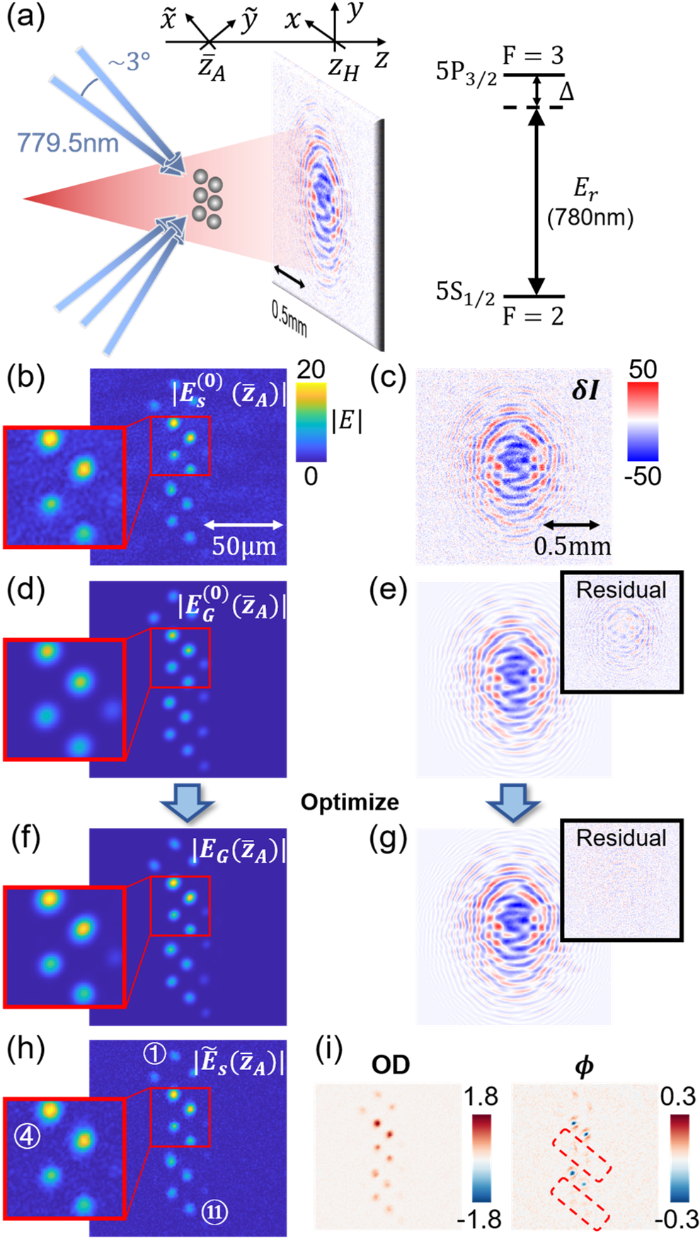
Figure 2: (a): Sketch of the experimental setup, typical hologram $\delta I$ at $\Delta\approx 0$, and the atomic level diagram. (b)-(c): Reduced hologram $\delta I$ (averaged over 9 exposures to enhance the display) and the modulus of $E_{s}^{(0)}(\bar{z}_{A})=\hat{U}(\bar{z}_{A}-z_{H})\left(\frac{\delta I}{E_{r}^{*}}\right)$ in $\bar{z}_{A}$ plane. (d)-(e): Initial Gaussian beams profile in the $z={\bar{z}}_{A}$ plane (plotted as $|E_{G}^{(0)}|$) and expected (reduced) hologram $\delta I_{e}$ in $z=z_{H}$. The sub-figure on (e) is the residual $\delta I_{e}-\delta I$. (f)-(g): Modulus of the optimal Gaussian profiles $E_{G}=\langle E_{s}(\bar{z}_{A})\rangle_{G}$ and the corresponding hologram. (h): Modulus of $\tilde{E}_{s}(\bar{z}_{A})$ with Gaussian-approximated twin image removed. Eleven samples are labeled from left to right, from top to bottom. (i): Reconstructed $\rm OD$, $\phi$ distributions. At $z=\bar{z}_{A}$, only the samples in dash-lined boxes are with the phase-shift $\phi$ rightly suppressed in-focus for $\Delta\ll\Gamma$.

III.2 Results

With the $\{I^{\prime},I\}-$hologram set and the pre-characterized $E_{r}$, We follow the procedure outlined in Sec. II to reconstruct $E_{s}$ using the Gaussian-decomposition method. To initiate the nonlinear optimization (Eq. (10)), we first directly propagate $E_{s}^{(0)}=\delta I/E_{r}^{*}$ to an estimated atomic sample plane $\bar{z}_{A}$. As evident from Eq. (3), with this step $E_{s}(\bar{z}_{A})$ can be focused, albeit being contaminated by a weak, defocused background associated with the “twin” term $E_{s,{\rm twin}}$ (Eq. (5)), as well as a typically even weaker “dc” $|E_{s}|^{2}/E_{r}^{*}$ term. Nevertheless, the preliminary $E_{s}^{(0)}(\bar{z}_{A})$ image in Fig. 2b helps us to initialize the $\{c_{j},{\bf P}_{j}\}$-parameter and compute $E_{G}^{(0)}$, as in Fig. 2d, with which we evaluate the expected (reduced) hologram $\delta I_{e}^{(0)}=E_{r}^{*}E_{G}^{(0)}+E_{r}{E_{G}^{(0)}}^{*}+{|E_{G}^{(0)}|}^{2}$ in Fig. 2e.

As by Eq. (10), the minimization of $\mathcal{L}_{\rm total}$ involves simultaneous minimization of $\mathcal{L}_{H}=\sum|\delta I_{e}-\delta I|^{2}$ and a set of $\mathcal{C}_{\mu}(\varphi(z_{A}))$ in $\mathcal{L}_{A}$ associated with the expected $\varphi_{A}$ distribution. In this step, we exploit spatial (Appendix B.2.1) and phase-uniformity (Appendix B.2.3) constraints. With $n_{A}=3$ Gaussians for each samples, the final Gaussian approximation $\langle E_{s}\rangle_{G}$ is displayed at $z=\bar{z}_{A}$ in Fig. 2f. The optimal $\delta I_{e}$ is shown in Fig. 2g. Finally, following Eq. (13), we obtain $\tilde{E}_{s}$ which is displayed in Fig. 2h at $z=\bar{z}_{A}$.

With $\tilde{E}_{s}\approx E_{s}$ and $E_{r}$ at hand, in Fig. 2i we evaluate $\varphi_{A}$ for all the samples at the fixed, “common” $z=\bar{z}_{A}$, and plot the OD and $\phi$ images. The array of samples are axially displaced by tens of micrometers. Here, with $\Delta\ll\Gamma$ we expect $\phi\ll{\rm OD}$ according to Eq. (18), which is satisfied for arrays of samples enclosed by dash-lined boxes only. For these samples, their $z_{A}$ are close enough to $\bar{z}_{A}$ in the display. For other samples, the out-of-focus images mixes ${\rm OD}$ with $\phi$, as expected.

III.2.1 Sample position localization

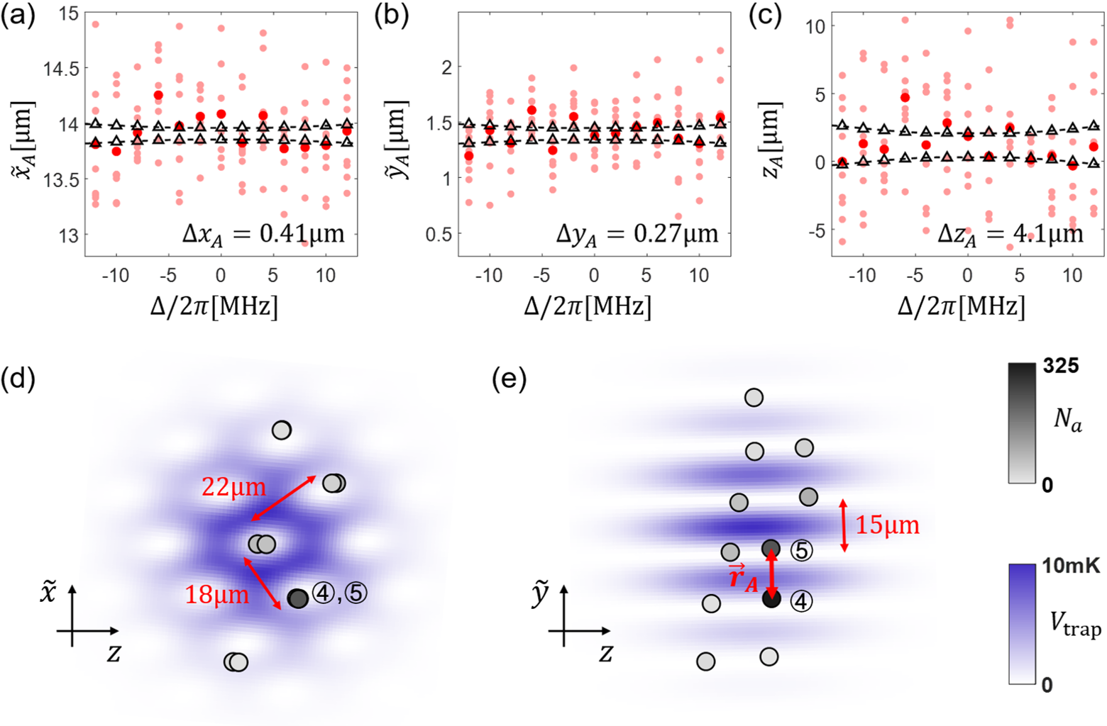
Figure 3: (a)(b)(c): Relative displacement between two samples marked in (d)(e) (and Fig. 2h) estimated with single-shot $\delta I$ using Eq. (39) criterion. The single-shot estimation at different probe detunings are plotted with red dots. Black triangles indicate the photon-shot-noise limits according to Eq. (29). The standard deviations ${\Delta x_{A}}$, ${\Delta y_{A}}$, ${\Delta z_{A}}$ in the figures are averaged over all data at detunings between $-12{\rm MHz}\leq\Delta/2\pi\leq 12{\rm MHz}$. (d)(e): Visualization of the sample locations in the 3D lattice. Here the locations are collectively decided by the phase angles [19] using Eq. (18) with the $4{\rm MHz}\leq|\Delta|/2\pi\leq 12{\rm MHz}$ data. The atom number $N_{a}$ is estimated by Eq. (18) with $\xi(s)\propto 1/(1+s)$ [72]. The circles represent the atomic samples with radius representing the sample sizes. The sizes are larger than $\Delta x_{A},\Delta y_{A}$, as well as the collectively-improved $\Delta z_{A}\leq 1.5\rm{\mu m}$.

With the $E_{s}$ decomposition based on single-shot $(I^{\prime},I)$ data, we obtain a list of $z_{A}$ and the low-resolution $\langle\varphi_{A}\rangle_{G}$ for each samples. Using $|\langle\varphi_{A}\rangle_{G}|$ in the $x-y$ plane, the center-of-mass locations ${\bf r}_{A}=\{x_{A},y_{A},z_{A}\}$ are retrieved. As being outlined in Sec. II, for the $z_{\sigma}\ll z_{A},z_{H}-z_{A}$ samples here, we refine the $z_{A}$ estimation simply by reconstructing $\tilde{E}_{s}$ with Eq. (13), and then re-applying the phase-angle uniformity criterion (Eq. (39)). Depending on the $E_{s}$ complexity and the $n_{A}$ exploited for the decomposition ($n_{A}=3$ here), the $\tilde{E}_{s}$-refinement generally leads to slightly improved $z_{A}-$estimation. Here, for samples with substantial ${\rm OD}$ and $\phi$, such as the $\leavevmode\hbox to11.37pt{\vbox to11.37pt{\text{[drawing]}}},\leavevmode\hbox to11.37pt{\vbox to11.37pt{\text{[drawing]}}}$ samples for Fig. 2(a-c) data, this refinement corrects small $\Delta-$dependent errors in $z_{A}$ by $2\sim 5~{}\mu$m.

To estimate the accuracy of the atomic sample localization, ideally we would like to analyze the fluctuation of the individual position values retrieved from repeated measurements. However, our sparse lattice is not stable enough. The lattice centers translate together by $1\sim 2~{}\mu$m from shot-to-shot, likely caused by pointing-instability of the lattice beams (Fig. 2a). While the fluctuation hardly impacts our axial, $z_{A}$-localization analysis, its suppression is required for analyzing the statistics on the more precisely located $x_{A},y_{A}$ values. To suppress the position fluctuation, in Fig. 3a-c we instead analyze the relative displacement between two samples. For the single-shot analysis we choose samples with largest atom numbers, marked as ”, ” according to Fig. 2h. In Appendix A we evaluate the shot-noise-limited precision to $\Delta{\bf r}_{A}$ as the classical Cramer-Rao bounds with $N_{s}=\sum_{x,y}|E_{s,A}|^{2}$ photons (Eq. (29)). We find the transverse $\Delta x_{A},\Delta y_{A}$ are about a factor of 5$\sim$6 larger than the $100~{}$nm-level photon shot-noise limit (Eq. (29)), which are likely due to shot-to-shot relative motion between the pair of samples. On the other hand, the 4 $\mu$m axial $\Delta z_{A}$ is a factor of 4 larger than the photon shot-noise limit (Eq. (29)). That the single-shot $\Delta z_{A}$ is quite far from the shot-noise-limit is likely related to non-optimal data analysis in presence of imaging noises. Nevertheless, both the transverse $\Delta x_{A}$, $\Delta y_{A}$, and the axial $\Delta z_{A}$, are already all well-below the diffraction limits set by $\lambda/{\rm NA}=3~{}\mu$m and $2\lambda/{\rm NA}^{2}=23~{}\mu$m, respectively.

Therefore, as in Fig. 3c, we are able to “super-resolve” $z_{A}$ for each sample with $\sim 10^{2}$ atoms even using a single-shot $(I^{\prime},I)-$data with $\tau_{p}=20~{}\mu$s exposure. The accuracy can be improved further by exploiting the spectroscopic constraint with the full $\{I^{\prime},I\}$ data set [19] collectively. In particular, by enforcing the ${\rm tan}\beta\propto\Delta$ relation required by Eq. (18) for all the data (except for $|\Delta|/2\pi<4~{}{\rm MHz}$ data, where the radiation pressure effect is most predominant, as following), our $z_{A}$ estimation is substantially improved. For the $\leavevmode\hbox to11.37pt{\vbox to11.37pt{\text{[drawing]}}},\leavevmode\hbox to11.37pt{\vbox to11.37pt{\text{[drawing]}}}$ samples, the $\Delta z_{A}$ are reduced to below one micrometer. Comparing with single-shot $z_{A}$ localization as in Fig. 3c, the refined $z_{A}$ typically involves 2-3 $\mu$m additional corrections. These corrections helps to ensure that the samples are more consistently located within dark centers of the 3D lattice, as illustrated in Figs. 3(d)(e).

III.2.2 Complex-valued spectroscopic imaging

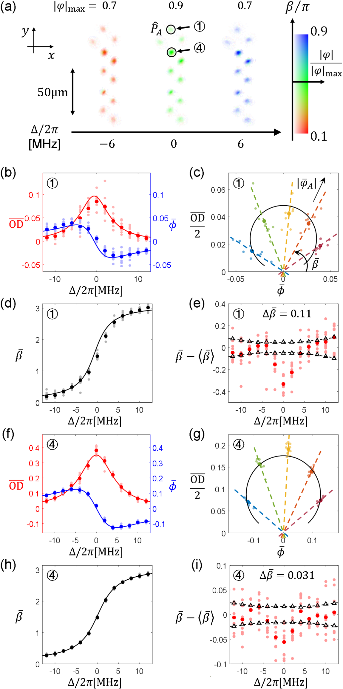
Figure 4: Complex-valued spectroscopic imaging. (a): Color domain plot of $\varphi_{A}$ with all the samples projected to the $z=\bar{z}_{A}$ plane. (b)(f): Average $\overline{\rm OD}$, $\overline{\phi}$, within $\hat{P}_{A}$ marked in (a), for ”1,4” samples respectively. Solid (transparent) dots are average (individual) values of nine measurements. Solid lines are fitted according to Eq. (18). (d)(h): The phase-angle spectroscopy. Notice in (h) the 9 sets of data overlap closely. (c)(g): $\overline{{\rm OD}}/2$-$\overline{\phi}$ phasor plot at $\Delta/2\pi=-6~{}{\rm MHz},-2~{}{\rm MHz},0~{}{\rm MHz},2~{}{\rm MHz}$ and $6~{}{\rm MHz}$, in red, orange, yellow, green, and blue respectively. The black lines are according to the (b)(f) fits. (e)(i): Residuals of $\bar{\beta}$ from the (d,h) fits. Black triangles and dashed lines give photon-shot-noise limit [18] (Eq. (9)). The phase-angle uncertainty $\Delta\bar{\beta}$ of $0.11$ and $0.031$ are averaged over $4{\rm MHz}\leq|\Delta|/2\pi\leq 12{\rm MHz}$ single shot data. The values are about a factor of two larger than the corresponding photon-shot-noise limit (Eq. (9)) [76].

With the list of $z_{A}$ and $\langle\varphi_{A}\rangle_{G}$ for each sample, we can proceed to evaluate $\tilde{E}_{s,A}$ with Eqs. (13)(16) and to approximately obtain $\varphi_{A}$ with diffraction-limited resolution, according to Eq. (2). However, as discussed in Appendix A, the Eq. (9) shot-noise-limit to the phase-angle $\beta$ is reached with fixed $z_{A}$. Without the knowledge, the phase-angle uncertainty $\Delta\beta$ is compromised by a factor of $1/\sqrt{2}$, at least. Therefore, we re-optimize the Gaussian decomposition, using the $\{I,I^{\prime}\}$-set, collectively improved $z_{A}$ as prior knowledge. The phase-angle spectroscopy to be discussed in the following is based on such re-optimized single-shot Gaussian decomposition (Fig. 3(d,e)).

We now evaluate $\varphi_{A}=\varphi(z_{A})$ using Eqs. (2)(16). The color-domain plots in Fig. 4a show $\varphi_{A}$, with phase angle $\beta$ indicated by color and modulus $|\varphi_{A}|$ by brightness. In contrast to Fig. 2(i), $\varphi(z_{A})$s from various samples are ”projected” to $z=\bar{z}_{A}$ from different $z_{A}$ planes. In the plots we observe consistent phase-angle $\beta$ at the same detunings $\Delta$, as anticipated. It is also observed that the same sample may appear slightly different at various detunings. This slight distortion in shape is primarily attributed to the lensing effect as the probe passes through the microscopic samples.

To further demonstrate aspects of the complex-valued spectroscopy, in Figs. 4(b)(f) we choose $\leavevmode\hbox to11.37pt{\vbox to11.37pt{\text{[drawing]}}},\leavevmode\hbox to11.37pt{\vbox to11.37pt{\text{[drawing]}}}$ samples and plot $\overline{\rm OD}=2{\rm Im}[\bar{\varphi}_{A}]$, $\overline{\phi}={\rm Re}[\bar{\varphi}_{A}]$ as a function of the probe detuning $\Delta$. Here $\bar{\varphi}_{A}$ is averaged over the sample area $\hat{P}_{A}$ as suggested in Fig. 4a. The same data is further presented in Figs. 4(c)(g) as 2D phasor plots, and in Figs. 4(d)(h) in terms of phase-angle spectroscopy.

In Figs. 4(b)(f) we see data from the repeated single-shot measurements fluctuate substantially. A closer look suggests there are strong correlations between the $\overline{\rm OD}$ and $\bar{\phi}$ fluctuations, which are more clearly seen in Figs. 4(c,g): The repeated measurements mostly spread the data points along the radial $|\varphi_{A}|$ direction instead of along $\beta$. These fluctuations are associated with the quite-expected atom number fluctuations in repeated measurements, which strongly affect the modulus $|\varphi_{A}|$ but hardly affect $\beta$, according to Eq. (18).

The $\beta$-stability is directly seen in the Fig. 4(d)(h) phase-angle plot. Here we use Eq. (18), with $\xi(s)\propto 1/(1+s)$, to fit the data. By excluding the $-4~{}{\rm MHz}<\Delta/2\pi<4~{}{\rm MHz}$ data points from the fit, $s_{0}\approx 1$ and $\Gamma\approx 6~{}$MHz can be extracted, agreeing excellently with expectation. The residuals are shown in Figs. 4(e)(i). Notably, for all the samples, we consistently see deviation of the $\bar{\beta}$-data from the 2-level model within $\Delta<\Gamma/2$. As in Sec. II.4, this deviation is caused by Doppler shifts associated with atomic motion. In particular, for the $\tau_{p}=20~{}\mu$s probe with $s_{0}=1$ on resonance, the atomic sample is expected to be accelerated to a final $v\approx 1$ m/s along ${\bf e}_{z}$. The average $k\overline{\Delta v}\sim 2\pi\times 640~{}$kHz Doppler shift is sensed by our complex spectroscopy, leading to $\delta\bar{\beta}=2k\overline{\Delta v}/\Gamma\approx 0.2$ shift to the phase angle, according to Eq. (18). Remarkably, the shift is almost halved for the sample, as in Fig. 4i, which is likely related to reduced radiation pressure [77] due to attenuation of the probe by the larger sample.

We note that on resonance the radiation pressure is also expected to displace the samples by up to $10~{}\mu$m along $z$. The average $z_{A}$ displacement is $2\sim 3~{}\mu$m-level at most. The differential displacement between $\leavevmode\hbox to11.37pt{\vbox to11.37pt{\text{[drawing]}}},\leavevmode\hbox to11.37pt{\vbox to11.37pt{\text{[drawing]}}}$ samples caused by the radiation pressure is below the axial resolution in Fig. 3(c).

We estimate the phase-angle resolution $\Delta\bar{\beta}(\Delta)$ using the data statistics from Fig. 4(e)(i). Theoretically, for optically thin samples, the resolution $\Delta\bar{\beta}(\Delta)$ is constrained by $N_{s}(\Delta)$ , which represents the number of coherently scattered photons $E_{s}$ received by the camera, through the Eq. (9) relation (Appendix A). After applying a moderate correction for finite $|\varphi_{A}|$ as discussed in ref. [18], the shot-noise-limited $\Delta\bar{\beta}$ values are evaluated according to Eq. (9) and marked with triangle symbols in Fig. 4(e)(i). We observe that the values of $\Delta\bar{\beta}$ closely follow the photon-shot-noise limit for both the and samples. By averaging the standard deviations of $\Delta\bar{\beta}(\Delta)$ across all data in Fig. 4, excluding the range $-4~{}{\rm MHz}<\Delta/2\pi<4~{}{\rm MHz}$, we estimate statistically the single-shot resolution to be $\Delta\bar{\beta}\approx 0.11$ and $0.031$ for the and samples, respectively [76]. For the sample, the 30 mrad resolution in $\beta$ suggests a frequency resolution of $\Delta\omega=2\pi\times 100~{}{\rm kHz}$, according to Fig. 4h and Eq. (18) near $\Delta=0$, where $\Delta\omega=\Delta\beta\times\Gamma/2$ and $\Gamma=2\pi\times 6{\rm MHz}$.

III.2.3 Field sensing

With the spectroscopic images of atomic arrays, it is possible to detect local perturbation to the $|g\rangle-|e\rangle$ transition frequency $\omega_{eg}$ in 3D with high spatial resolution. In this section, we demonstrate this field-sensing capacity by measuring the transition light shift induced by a “dressing” laser. The schematic setup is displayed in Fig. 5a. Right before the imaging exposure, a dressing laser $E_{m}$ with a Gaussian radius of $w_{m}\approx 10~{}\mu$m, at $\lambda_{m}=1064~{}$nm and with power $P_{m}\approx 1~{}$W, is turned on. This leads to Stark shift $\delta\omega_{eg}\propto{|E_{m}|}^{2}$ of about 6 MHz. The shift is clearly seen in Fig. 5b with the $\varphi_{A}$ images.

Taking a closer look at Fig. 5b, since the dressing beam is not uniform, the 3D-distributed samples experience slightly different $\delta\omega_{eg}$ shifts. In Fig. 5c we plot $\bar{\beta}={\rm arg}(\bar{\varphi}_{A})$ for three samples, labeled as , , in Fig. 5b. For the convenience of display, we encode the sample index with the degree of transparency for the $\bar{\beta}$ curves. We clearly see that while in absence of dressing the $\bar{\beta}$ curves closely overlap (the red curves), the three $\bar{\beta}$ curves disperse apart when $E_{m}$ is on (blue curves). The difference is most pronounced near the shifted $\omega_{eg}$ center, with $\Delta/2\pi\approx 6~{}$MHz, where $\bar{\beta}$ regains the highest $\Delta$-sensitivity of $\partial_{\Delta}\beta\sim 2/\Gamma$ according to Eq. (18). By analyzing the spectra for all samples, we are able to resolve $\delta\omega_{eg}$ in 3D with micro-meter resolution. The spatial-dependent light shift is most conveniently displayed in the $x-z$ plane where the dressing beam is in focus. For the purpose, the vertical view of $\Delta\omega_{eg}$ is plotted in Fig. 5d for our eleven samples with significant $|\varphi_{A}|$.

The field-sensing capacity demonstrated in this section shares the same frequency resolution with that is discussed in the last section. In particular, according to Eq. (18) near the shifted $\omega_{eg}$ resonance, we again have $\Delta(\delta\omega_{eg})/2\pi\approx 100~{}{\rm kHz}$. We emphasize this resolution is achieved by $\sim 10^{2}$ atoms within $\tau_{p}=20~{}\mu$s, with micron-sized 3D resolution.

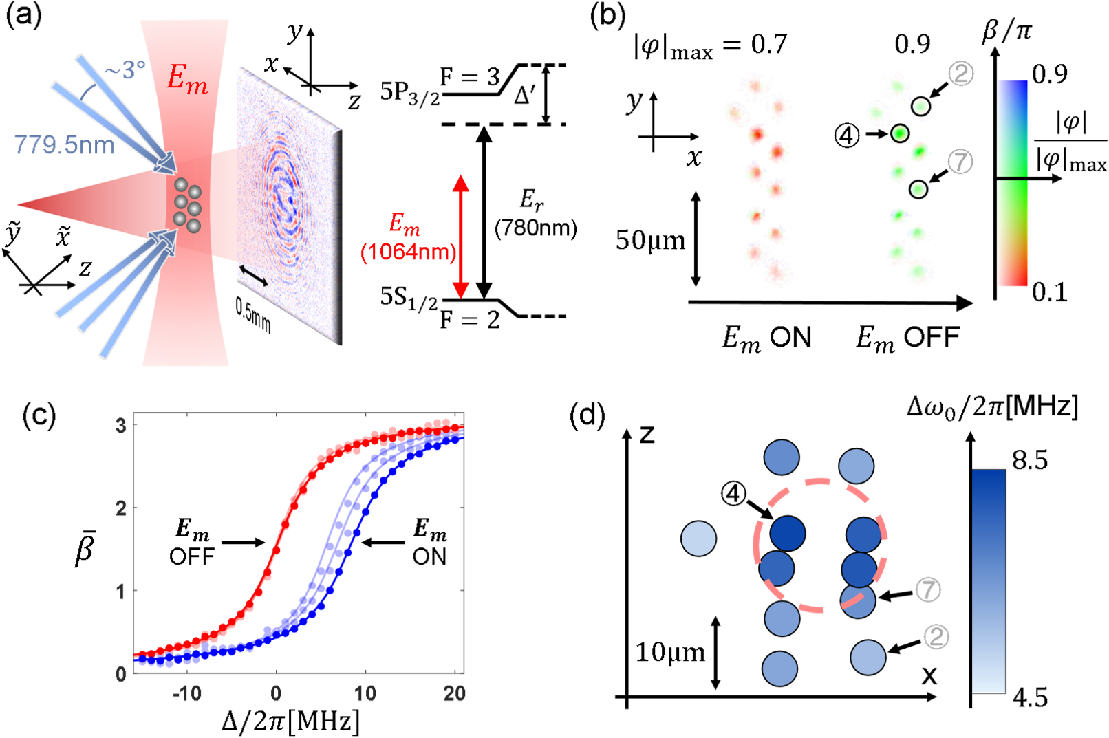
Figure 5: Sensing light shifts with a sparse array of laser-cooled atoms. (a): Experimental setup and the level diagram. (b): $\bar{z}_{A}$-projected $\varphi_{A}$-images of the axially displaced samples, with and without $E_{m}$. The data are processed from $\delta I$ averaged over 9 exposures to enhance the display. The probe detuning is $\Delta/2\pi=0~{}{\rm MHz}$. (c): $\hat{P}_{A}$-averaged phase angle spectra of ”2,4,7” samples marked in (b). The red (blue) curves are for $E_{m}$ off (on). The transparency levels are according to the markers in (b). (d): $x-z$ “top” view of the light shift distribution. The 11 largest-$|\varphi|$ samples are represented by blue disks. The dash-lined circle suggests the estimated $E_{m}$ full-width-half-maximum focal spot in the $x-z$ plane.

IV Discussions

IV.1 Aberrations

So far, our holographic imaging scheme assumes aberration-free propagation of $E_{r}$, $E_{s}$ between the sample plane $z_{A}$ and hologram plane $z_{H}$. Practically, the $E_{r,s}$ wavefronts need to be optically relayed from the ultrahigh vacuum to the place where the digital camera sensor conveniently locates. For high-NA imaging, aberration becomes unavoidable when the required volume-of-view is large.

To describe the imperfect imaging, we consider both $E_{r}$ and $E_{s}$ as in Fig. 1a to be relayed from inside the ultrahigh vacuum where the actual light-atom interaction takes place. We use a wavefront propagator $U_{\rm img}$ to generally represent the linear transformation of wavefronts from the in-situ $z=z_{V,A}$ to $z=z_{A}$,

$$E_{r}(x,y,z_{A}) ={U}_{\rm img}E_{r}(x_{V},y_{V},z_{V,A}),$$ (19)

$$E_{s}(x,y,z_{A}) ={U}_{\rm img}E_{s}(x_{V},y_{V},z_{V,A}).$$

For imperfect imaging, the fundamental way to eliminate the associated imaging errors is to fully characterize the propagator $U_{\rm img}$. Then, by resolving $E_{r,s}(z_{V,A})$ through Eq. (19) to apply our prior knowledge about the samples in situ. Practically, even with advanced computing power, the modeling of diffraction-limited $E_{r},E_{s}$ propagation across the large-diameter lens-array can still be prohibitively resource-demanding. On the other hand, the wavefront propagation is greatly simplified by Gaussian decomposition [32, 33, 34]. The well-developed technique is naturally adapted to the Gaussian-assisted holography scheme in this work to potentially enable aberration-free imaging of sparse samples over unprecedentedly large imaging volumes, only limited by the finest hologram fringes that can be captured by the camera [68].

To fully characterize $U_{\rm img}$ for the large-diameter lens-arrays [73, 74], and to invert Eq. (19) with Gaussian-decomposition, are all beyond the scope of this work. Instead, we take advantage of the small volume-of-view (Fig. 2) to address minor, aplanatic aberrations. This is achieved by employing a point-spread function [43] $O(x,y)$ through in situ optical measurements. The procedure is detailed in Appendix D.3.

IV.2 Speckles

In addition to aberrations, the imaging optics may introduce speckle noise into the wavefronts through multiple reflections and even by small dusk particles on the optical surfaces. Since the probe beam for atomic spectroscopy is highly monochromatic, the speckle noises are difficult to avoid.

We denote $\delta E_{r}$ and $\delta E_{s}$ to be speckle fields generated by unwanted reflections and scatterings across the imaging optical path. We assume that the perturbations are static enough for their precise characterization through multiple measurements. With Gerchberg-Saxton iterations [18], $\delta E_{r}$ is fully characterized in this work (Fig. 1b). When speckle noises in $E_{r,s}$ are moderate, as in this work, their presence hardly affect our prior knowledge about $\varphi_{A}$ for the $E_{s}$ retrieval (Sec. II). But the presence of $\delta E_{r}$ does affect the $\varphi_{A}$ retrieval with Eqs. (2), particularly since substantial amount of the speckle noises $\delta E_{r}$ may be generated by imaging optics after the light-atom interaction, not “seen” by atoms at $z=z_{A}$. To minimize the $\delta E_{r}$ impact, one should locate the sources of $\delta E_{r}$ with digital propagation of $E_{r}$, and by removing the speckles to recover the actual $E_{r}$ attending the light-atom interaction. The process of characterizing the speckle sources across the imaging path is therefore similar to characterizing $U_{\rm img}$ discussed above. If all the speckle scatterings in $\delta E_{r,s}$ are static enough, the procedure would help to fully suppress the associated noises in the $\varphi_{A}$ retrieval.

In this work, we take a simpler approach to approximately suppress the speckle noise to the complex-valued spectroscopic imaging. In particular, during the Eq. (2) evaluation of $\varphi_{A}$, we simply filter away the apparent speckles from $E_{r}$. This is achieved by digitally focusing $E_{r}$ back to $z=0$ and only choose a small region around the diffraction-limited component, before propagating forward to $z=z_{A}$ for the $\varphi_{A}$ evaluation. In other words, we assumes $E_{r}$ “seen” by atoms is speckle-less, which is a good approximation in our setup, considering that comparing to the multiple-stage-relayed large-diameter imaging optics, the $E_{r}$ is focused to atomic samples with simpler, smaller-diameter optics [73].

IV.3 Summary

From precision spectroscopy [78, 61, 62] to quantum simulation [79], precise optical imaging [80, 81, 82] is crucially important for advancing ultracold atomic physics research at frontiers. The prevailing imaging method in these researches is to directly record fluorescence [83, 80, 81, 84], absorption [85, 17], and phase shift [20]. While holographic imaging techniques are rapidly developing for applications in other fields [59, 86, 87, 67], their utilities in atomic physics are rare [40, 41, 30, 42, 43, 18]. In Sec. I.2 we highlighted major challenges of quantitative holographic imaging for precision spectroscopic measurements of cold atoms. In Sec. I.3.1 we provided arguments that the 3 dB information loss in holographic measurements hardly make them disadvantageous when comparing to direct imaging. If the challenges can be addressed, then, by extending the spectroscopy data to complex numbers and by enabling 3D resolution, the holographic method would help to unlock highly exciting opportunities associated with precise spectroscopic imaging and sensing on strong optical transitions.

In this work, motivated by the exciting prospect of complex-valued 3D spectroscopic imaging, we develop a systematic approach to address key challenges in holographic imaging of cold atoms (Sec. I.2). Comparing with e.g. biological applications [46, 88], our choices of schemes and diversities in holographic measurements are severely constrained by aspects of cold-atom setups. Our philosophy is to fully characterize the imaging setup and to efficiently utilize all the available knowledge from single-shot inline holography. The efficient application of prior knowledge is numerically assisted by Gaussian beam propagation, a simple application of the well-established Gaussian-decomposition technique [32, 89, 33, 34, 90]. With the method, we have demonstrated complex-valued spectroscopic imaging of axially displaced microscopic ⁸⁷Rb samples in a sparse lattice, with micrometer 3D resolution. We achieve hundred-kHz-level single-shot frequency resolution out of the $\Gamma/2\pi=6~{}$MHz natural linewidth, with merely hundreds of atoms, a result that appears extremely difficult to realize with traditional spectroscopy [1, 62], in presence of atom number and interaction strength uncertainties.

Not discussed in this paper is the observation of atomic shot noise [17, 43], which is barely supported by but nevertheless observed with our ${\rm NA}\approx 0.26$ setup. In addition, the imaging volume-of-view in this work is limited by the sample distribution itself to be within a $\sim$100$~{}\mu$m distance (Also see Appendix E). We clarified in Sec. IV.1 that the technique can be extended to fully suppress wavefront aberrations for wide-field 3D imaging [91] of sparse atomic samples. The development may enable wideband, spectroscopic sensing of 3D potentials [15, 92] with unprecedented volume-of-view. Other than probing single-atom spectroscopic responses, our method also supports the study of resonant dipole interactions by simultaneously measuring the strength, direction and phase angle of the collective emission [25, 93]. As such, we also expect the complex-valued spectroscopic imaging method to facilitate efficient characterization and quantum engineering of advanced light-atom interfaces [78, 94, 95, 96, 97].

Appendix A Cramer-Rao bounds to position and phase localization by inline holography

In this section, we consider the estimation of bulk properties of the atomic sample from the hologram $I,I^{\prime}$ specified in Eq. (3). The basic setup is illustrated in Fig. 1a. The bulk properties of interest include the 3D atomic central locations ${\bf r}_{A}=\{x_{A},y_{A},z_{A}\}$ and the total amplitude of the forward scattering $E_{s}$. To facilitate the derivations, we introduce five $\{\theta_{j}\}=\{x_{A},y_{A},z_{A},\beta_{r,{\rm off}},\beta_{i,{\rm off}}\}$ parameters. The last two parameters are the real and imaginary parts of an auxiliary complex phase offset in

$$\tilde{E}_{s}=e^{i\beta_{\rm off}}\hat{U}(z_{H}-z_{A})\left(E_{r}(z_{A})(e^{i\varphi_{A}}-1)\right).$$ (20)

For example, with $|\varphi_{A}|\ll 1$, then $\beta_{r,{\rm off}}$ offsets our estimation to phase-angle $\beta={\rm arg}[\varphi_{A}]$, and $\beta_{i,{\rm off}}$ offsets $|\varphi_{A}|$.

The hologram $I$ is accordingly re-modeled as

$$\tilde{I}=\left|E_{r}(z_{H})+\tilde{E}_{s}\right|^{2}$$ (21)

so that $I^{\prime}=\tilde{I}|_{\beta_{\rm off}\rightarrow 0}$. We regard $p(x,y)=\tilde{I}(x,y)/\sum_{x,y}\tilde{I}(x,y)$ as a 2D probability distribution of a single photon received by the camera. The Fisher information matrix is accordingly expressed as

$$F_{jk}^{(0)} \equiv\left(\sum_{x,y}\frac{1}{p(x,y)}\partial_{\theta_{j}}p(x,y)\partial_{\theta_{k}}p(x,y)\right)_{\beta_{\rm off}\rightarrow 0},$$ (22)

$$\approx\left(\frac{\sum_{x,y}\frac{1}{\tilde{I}(x,y)}\partial_{\theta_{j}}\tilde{I}(x,y)\partial_{\theta_{k}}\tilde{I}(x,y)}{\sum_{x,y}\tilde{I}(x,y)}\right)_{\beta_{\rm off}\rightarrow 0}.$$

In the second line of Eq. (22) we assumed the total flux $\sum_{x,y}\tilde{I}(x,y)$ received by the camera to be $\theta_{j}$-independent, which is sufficiently satisfied for moderately-dense atomic samples in the defocused-twin regime (Appendix C.1) with $z_{\sigma}\ll z_{A},z_{H}-z_{A}$ (Fig. 1a), so that $|E_{s}|\ll|E_{r}|$ on the camera plane as to be assumed in the following. With $\partial_{\theta_{j}}\tilde{I}\partial_{\theta_{k}}\tilde{I}\approx|E_{r}|^{2}(\partial_{\theta_{j}}\tilde{E}_{s}^{*}\partial_{\theta_{k}}\tilde{E}_{s}+c.c)+(E_{r}^{*2}\partial_{\theta_{j}}\tilde{E}_{s}\partial_{\theta_{k}}\tilde{E}_{s}+c.c.)$, the second term also vanishes upon the 2D integration, due to the substantial wavefront mismatch between $E_{r}$ and $E_{s}$. Equation (22) is accordingly simplified into

$$F_{jk}^{(0)}\approx\frac{\sum_{x,y}\left(\partial_{\theta_{j}}\tilde{E}_{s}^{*}\partial_{\theta_{k}}\tilde{E}_{s}+c.c.\right)_{\beta_{\rm off}\rightarrow 0}}{\sum_{x,y}|E_{r}|^{2}}.$$ (23)

The Fisher information matrix by Eq. (23) is associated with single-photon detection on the camera. For imaging cold atoms, we are more interested in Fisher information associated with photons scattered by the samples [98]. A change of normalization leads to

$$F_{jk}=\left(\frac{\sum_{x,y}\partial_{\theta_{j}}\tilde{E}_{s}^{*}\partial_{\theta_{k}}\tilde{E}_{s}+c.c.}{\sum_{x,y}|\tilde{E}_{s}|^{2}}\right)_{\beta_{\rm off}\rightarrow 0}.$$ (24)

Interestingly, Eq. (24) suggests Fisher information for holographic measurements upon a single $E_{s}$-photon detection is equal to half of the quantum Fisher information [35] for the $E_{s}$-photon wavepacket. This 50% loss of information is generally associated with heterodying measurements [30].

From a single photon wavepacket to $N_{s}=\sum_{x,y}|E_{s}|^{2}$ photons detected by the camera in an uncorrelated manner, we have $F_{jk}(N_{s})=N_{s}F_{jk}$ according to Eq. (24) to limit the resolutions of $\{\theta_{j}\}$ measurements with the associated Cramer-Rao bounds. With Eq. (20), evaluation of Eq. (24) for the $\beta_{r,{\rm off}}$, $\beta_{i,{\rm off}}$ differentiation is straightforward. With the free-space propagator $\hat{U}(z_{H}-z_{A})$ by Eq. (47) to be $x_{A},y_{A}$ independent, the translational invariance suggests

$$\partial_{x_{A}}\tilde{E}_{s}=-\partial_{x}\tilde{E}_{s},$$ (25)

$$\partial_{y_{A}}\tilde{E}_{s}=-\partial_{y}\tilde{E}_{s}.$$

For the differentiation of the $z_{A}-$parameter in Eq. (24), we rewrite

$$\tilde{E}_{s}=e^{i\beta_{\rm off}}\hat{U}(z_{H}-z_{A})\left(\left(\hat{U}(z_{A})E_{r}(0)\right)(e^{i\varphi_{A}}-1)\right).$$ (26)

Here the first propagator $\hat{U}(z_{H}-z_{A})$ acts on $E_{s}(z_{A})=E_{r}(z_{A})(e^{i\varphi_{A}}-1)$. The second $\hat{U}(z_{A})$ acts on $E_{r}(0)$ only. In the $z_{\sigma}\ll z_{A}$ (Fig. 1a) limit, the $E_{r}(z_{A})$ “seen” by the $\sigma-$sized atomic sample can be approximated by plane wave. For on-axis samples we therefore find

$$\partial_{z_{A}}\tilde{E}_{s}\approx i(-\sqrt{k_{0}^{2}+\partial_{x}^{2}+\partial_{y}^{2}}+k_{0})\tilde{E}_{s}.$$ (27)

With Eqs. (20)(25)(27), evaluation of Eq. (24) becomes straightforward for specific imaging setup, $E_{r}-$illumination, and atomic samples. To provide the Cramer-Rao bounds with a simple example, in the following we consider $E_{r}$ to propagate along the $z-$axis, $E_{s}(z_{A})$ to be the forward scattering by a Gaussian shaped sample located on the $z-$axis with a density distribution of $\rho_{c}=\rho_{0}e^{-(x^{2}+y^{2})/\sigma^{2}}$. We assume $\varphi_{A}=k_{0}\rho_{c}\alpha(\omega)\ll 1$ so that the $E_{s}$ amplitude simply follows the $\rho_{c}$ profile, while $\sigma>\lambda/{\rm NA}$ so that $E_{s}$ is almost fully captured by the camera. By normalizing $x_{A},y_{A}$ with $\sigma$, and $z_{A}$ with $z_{\rm\sigma}$, the rescaled Fisher information matrix with $N_{s}$ scattered-photon detection is

$$F(N_{s})=N_{s}\left[{\begin{array}[]{ccccc}2&0&0&0&0\\ 0&2&0&0&0\\ 0&0&1&1&0\\ 0&0&1&2&0\\ 0&0&0&0&2\\ \end{array}}\right].$$ (28)

Clearly, while $x_{A},y_{A}$ and $\beta_{i,{\rm off}}$ measurements are independent, the axial position $z_{A}$ is correlated with the phase angle $\beta_{r,{\rm off}}$. By diagonalizing Eq. (28) and evaluate the Cramer-Rao bounds indirectly using the eigenvector observables, one finds that in the $\varphi_{A}\ll 1$ optically-thin-sample limit,

$$\Delta x_{A} =\sigma/\sqrt{2N_{s}},$$ (29)

$$\Delta y_{A} =\sigma/\sqrt{2N_{s}},$$

$$\Delta z_{A} =z_{\sigma}/\sqrt{N_{s}/2},$$

$$\Delta\beta =1/\sqrt{N_{s}},$$

$$\Delta|\varphi_{A}| =1/\sqrt{2N_{s}}.$$

The axial resolution $\Delta z_{A}$ can be enhanced to $\Delta z_{A}=z_{\sigma}/\sqrt{N_{s}}$ limit (Eq. (8)) [19] by taking multiple spectroscopic measurements to fix $\beta$ first. On the other hand, with the axial position $z_{A}$ fixed, the phase angle resolution for the sample is enhanced to $\Delta\beta=1/\sqrt{2N_{s}}$ (Eq. (9)) [18].

Appendix B Details of Gaussian decomposition

B.1 Gaussian beam

Gaussian decomposition is associated with a class of powerful semi-classical wave-propagation techniques [32, 89, 33, 34, 90]. We focus on the free Gaussian-propagation to support evaluation of $E_{r},E_{s}$ across $z-$planes during the minimization of $\mathcal{L}_{\rm tot}$ in Eq. (10).

The standard form of a Gaussian beam is expressed as

$$G_{z}({\bf r};{\bf P}^{\prime})=e^{i({\bf r}_{\perp}-{\bf r}_{\perp}^{0})^{T}\frac{k_{0}}{{2\bf q}(z)}({\bf r}_{\perp}-{\bf r}_{\perp}^{0})+ik_{0}z+i\varphi_{G}(z)}.$$ (30)

Here ${\bf r}_{\perp}=(x,y)^{T}$. The complex ${\bf q}(z)$-parameter is defined by

$$\frac{1}{{\bf q}(z)}=\left[{\begin{array}[]{cc}\frac{1}{R_{x}}+i\frac{2}{k_{0}w_{x}^{2}}&0\\ 0&\frac{1}{R_{y}}+i\frac{2}{k_{0}w_{y}^{2}},\\ \end{array}}\right].$$ (31)

with

$$w_{c}(z) =w_{c}^{0}\sqrt{1+\frac{(z-z_{c}^{0})^{2}}{(z_{c}^{R})^{2}}},$$ (32)

$$R_{c}(z) =z-z_{c}^{0}+\frac{(z_{c}^{\rm R})^{2}}{z-z_{c}^{0}},$$

all decided by the Gaussian waists $w_{c}^{0}$ for $c=x,y$. The Gouy phase $\varphi_{G}(z)$ is given by

$$\varphi_{G}(z)=\frac{1}{2}\sum_{c=x,y}{\rm arctan}((z-z_{c}^{0})/z_{c}^{R}).$$ (33)

The Rayleigh lengths are defined as

$$z_{c}^{\rm R}=\pi(w_{c}^{0})^{2}/\lambda$$ (34)

for $c=x,y$.

Next, we introduce a rotation matrix $\mathcal{R}({\gamma})$ with Euler angles $\gamma=(\theta_{1},\theta_{2},\theta_{3})$, so that ${\bf k}=(0,0,k_{0})\mathcal{R}(\gamma)$ is expressed as

$${\bf k}=(-{\rm sin}\theta_{2},{\rm sin}\theta_{1}{\rm cos}\theta_{2},{\rm cos}\theta_{1}{\rm cos}\theta_{2})k_{0}.$$ (35)

The rotation angle $\theta_{3}$ orients the principal axis of the 2D Gaussian profile. With ${\bf r}=(x,y,z)^{T}$, we have

$$G({\bf r};{\bf P})=G_{z}(\mathcal{R}^{T}(\gamma){\bf r};{\bf P}^{\prime}).$$ (36)

Overall, with ${\bf P}=\{\gamma,{\bf P}^{\prime}\}$, there are a total number of nine parameters ${\bf P}=\{\theta_{1},\theta_{2},\theta_{3},x^{0},y^{0},z_{x}^{0},z_{y}^{0},w_{x}^{0},w_{y}^{0}\}$ for a 2D Gaussian beam. To decompose a wavefront into $n_{A}$ beams as in Eq. (7) involves a total number of $11\times n_{A}$ real parameters $\{c_{j},{\bf P}_{j}\}$.

B.2 Implementing the sample constraints

For a single sample as in Fig. 1 as well as multiple samples, our prior knowledge about the sample can often be formulated into a list of cost-functions $C_{\mu}$ to constrain the expected 2D complex-valued phase shift distribution, $\varphi(z_{A})=\varphi_{A}$. The constraints help to fix the phase-ambiguity associated with $E_{s,{\rm twin}}$ while locating the sample planes at $z=z_{A}$. In the following we provide examples of such $C_{\mu}$-constraints, generalized for multiple samples.

B.2.1 Finite spatial support

The prior knowledge on the regime of interest where the atomic samples should be constrained within, as schematically illustrated in Fig. 1c with $\hat{P}_{A}$, is a condition commonly applied for coherent imaging [58, 99, 30, 29]. Here, for multiple atomic samples, the constraint can be formulated as a request to minimize the cost function,

$$C_{\mu}=\sum_{A}\frac{1}{\mathcal{N}_{A}}\sum_{x,y}|\varphi(z_{A})-\hat{P}_{A}\left(\varphi(z_{A})\right)|^{2}.$$ (37)

Here $\mathcal{N}_{A}=\sum_{x,y}|\hat{P}_{A}(\varphi(z_{A}))|^{2}$ normalizes the error signal from each sample at the respective $z=z_{A}$.

B.2.2 Known phase angle

As being outlined in Sec. I and discussed in Sec. II.4, for complex-valued atomic spectroscopy of a dilute gas, the phase angle $\beta={\rm arg}(\varphi_{A})$ is often decided by the polarizability of single constituent atoms, $\beta_{0}={\rm arg}(\alpha)$, and is therefore precisely known. The knowledge can be applied to constrain the $\langle E_{s}\rangle_{G}$-search by minimizing

$$C_{\mu}=\sum_{A}\frac{1}{\mathcal{N}_{A}}\hat{P}_{A}\sum_{x,y}\left|{\rm Im}[\varphi(z_{A})e^{-i\beta_{0}}]\right|^{2}.$$ (38)

That is, by unwrapping the known phase angle $\beta_{0}$ from the complex-valued phase shift, $\varphi_{A}e^{-i\beta_{0}}$ should be real, with vanishing imaginary component across each sample.

The Eq. (38)-minimization is a generalization to previous phase angle constraints in holographic microscopy, such as positive attenuation criterion [60] and phase object criterion [42]. Application of Eq. (38) requires the phase angle $\beta=\beta_{0}$ as precise prior knowledge. Practically, $\beta_{0}$ can be obtained by pre-characterization of standard samples first [19]. In particular, for free atoms, $\beta_{0}(\Delta)$ can be fixed by exploiting the Eq. (18) relation across the atomic resonance under study first (during which the axial location $z_{A}$ for the standard samples are fixed too, as in Sec. III.2.1).

B.2.3 Phase-angle uniformity

Without the precise $\beta_{0}$ knowledge, one still can exploit prior knowledge on $\beta$ in holography. A common situation is that the atomic sample is monomorphous [41], with a uniform albeit not-precisely-known $\beta={\rm arg}(\varphi_{A})$ across the sample. The condition can be formulated as to minimize

$$C_{\mu}=\sum_{A}\frac{1}{\mathcal{N}_{A}}\hat{P}_{A}\left(|\sum_{x,y}\varphi(z_{A})|-\sum_{x,y}|\varphi(z_{A})|\right)^{2}.$$ (39)

B.2.4 Other types of constraints

Beyond the simple examples by Eqs. (37)(38)(39), more sophisticated form of prior knowledge about the samples can be applied to tailor the cost functions $C_{\mu}(\varphi)$. For example, the finite support in Eq. (37) can be replaced by a continuously varying $\hat{P}_{A}$ according to our expectation of the sample shape. Similar strategies can be applied to soften the $\beta_{0}$ bounds in Eq. (38) [60]. Other cost functions may be tailored to encourage the $\varphi(z_{A})$ distribution meeting our expectation of a mixed spatial-spectral characteristics, such as for atomic samples confined by a dipole trap [100].

B.3 Direct constraints

B.3.1 Direct constraints to Gaussian parameters

Instead of formulating $C_{\mu}$ cost functions, simple knowledge about the sample can also be applied as direct constraints to the Gaussian parameters. For example, the finite spatial support in Eq. (37) can be effectively enforced by limiting the range of ${\bf r}_{A}$ and $w_{x}(z_{A}),w_{y}(z_{A})$ parameters (Eq. (36)). As another example, in the $|\varphi(z_{A})|\ll 1$ weak scattering limit the phase-angle relation by Eq. (39) effectively enforce the wavefront radii of curvature $R_{x}(z_{A}),R_{y}(z_{A})$ to follow the $\langle E_{r}\rangle_{G}$ values.

B.3.2 Wavefront templates

Direct constraints to groups of Gaussian parameters become particularly useful when the $E_{s}$ is expected to be characterized by certain wavefront template. Examples include synthesizing the point-spread-functions of high-NA microscopes [101], or for finely matching the expected shape of an interacting degenerate gas [102]. To form the template, the Gaussian-decomposition of the wavefront template is generally expressed as

$$\tilde{G}_{\rm template}({\bf r})=\sum_{g}c_{g}G({\bf r};{\bf P}_{g}).$$ (40)

The $\tilde{G}_{\rm template}$ with correlated Gaussian parameters $\{c_{g},{\bf P}_{g}\}$ then enters the $\mathcal{L}_{\rm tot}$-minimization, together with other individual Gaussian beams if necessary.

B.3.3 Beyond paraxial

Finally, the Gaussian propagation by Eq. (31) is based on paraxial approximation which limits the propagation distance $L$ to $L\ll(z^{R}_{c})^{2}/\lambda$. To enhance the distance of faithful propagation, any Gaussian beam that is tightly focused around $z=z_{A}$ can be expanded into a superposition of weakly focused Gaussians according to Eqs. (36)(40).

Appendix C Out-of-focus effects

C.1 Defocused-twin regime

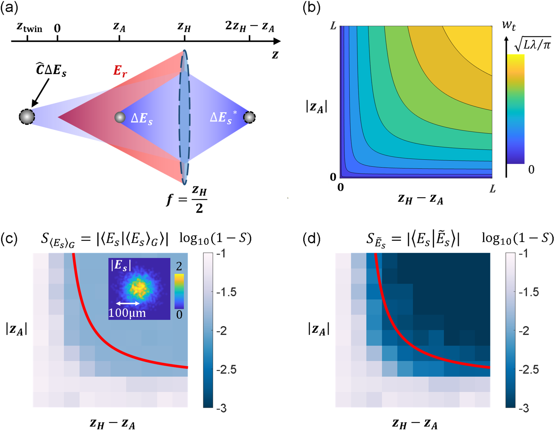
Figure 6: (a): Schematic diagram of the geometric relation between image and twin image when $z_{A}\textless z_{H}/2$. The ${\Delta E_{s}}^{*}$ is a mirror-image of $\Delta E_{s}$ at the other side of the holographic plane $z_{H}$. For spherical $E_{r}$, the $E_{r}/{E_{r}}^{*}$ term acts as a numerical lens with a focal length $f=z_{H}/2$. (b): The critical Gaussian beam size $w_{t}$ as a function of $z_{A}$ and $z_{H}-z_{A}$. (c): Fidelity of reconstructing $E_{s}$ using the Gaussian $E_{G}$ (Eq. (7)) approximations (Eq. (45)). Here the simulated $E_{s}$ follows a Gaussian profile with pixel-wise, Poissoinian atomic shot noise. The atom number is set to be 3500 in the simulation. The plot is averaged over 16 $E_{s}$ simulations. The red line sets the critical Gaussian $w_{t}$. A typical numerically generated $E_{s}$ from such a sample is given in the inset. (d): Fidelity plot similar to (c) but with $\langle E_{s}\rangle_{G}$ replaced by $\tilde{E}_{s}$ (Eq. (16)) to substantially improve the accuracy.

In the Fig. 1a inline setup with the spherical $E_{r}$ illumination, the twin-image $E_{s,{\rm twin}}$ (Eq. (5)) is paraxially focused to $z=z_{\rm twin}$. With $z_{\sigma}\ll z_{A},z_{H}-z_{A}$, the $E_{s,{\rm twin}}$ is sufficiently defocused at $z=z_{A}$. In absence of imaging noise, isolation of $E_{s}$ from $E_{s,{\rm twin}}$ becomes possible by limiting the $E_{s}$ location $\hat{P}_{A}$ with tight enough size of order $\sigma$ [58]. We refer this inline holography regime that supports simple twin-image removal as “defocused-twin regime”. In the following we exploit Gaussian optics to derive a characteristic Gaussian width $w_{t}$, as a function of $z_{A}$ and $z_{H}-z_{A}$, that sets the boundary of this regime for imaging small samples.

We consider that in the Fig. 1a setup the numerical reconstruction of certain $E_{s}$ is contaminated by an error term $\Delta E_{s}$, which is itself a Gaussian beam with complex radius of curvature $q=\frac{1}{a+ib}$ at $z=z_{A}$. Within the paraxial approximation, the twin image, expressed as $\Delta E_{s,\rm twin}=\Delta E_{s}^{*}E_{r}/E_{r}^{*}$ at the camera plane $z=z_{H}$, is also a Gaussian. We evaluate the twin profile $\Delta E_{s,\rm twin}$ at $z=z_{A}$ in four steps: propagation $\Delta E_{s}$ to $z_{H}$ plane; taking the complex conjugation; passing through an ideal thin lens with a focal length of $z_{H}/2$; and propagating to $z=z_{A}$ plane. The complex curvature of the $\Delta E_{s,\rm twin}$ at $z=z_{A}$ is given by:

$$q_{\rm twin}=\frac{q(2z_{A}-z_{H})+2z_{A}(z_{H}-z_{A})}{2z_{A}-z_{H}-2q}$$ (41)

Now, if $|\Delta E_{s}|\ll|E_{r}|$, then it is easy to show that the artifact field $E_{\rm arti}=(\Delta E_{s}-\Delta E_{s}^{*}E_{r}/E_{r}^{*})$ can be added freely to $E_{s}$ without affecting the expected hologram $I_{e}=|E_{r}+E_{s}|^{2}$. In other words, if the hologram data $(I,I^{\prime})$ and $E_{r}$ are all the prior knowledge we have, then the $E_{\rm arti}$ term is free to contaminate $E_{s}$ during its reconstruction. However, if $\hat{P}_{A}$ has a width that is smaller than the smallest possible $E_{\rm arti}(z_{A})$, then all the artifacts $E_{\rm arti}$ can be excluded. Here, the minimal width of $E_{\rm arti}(z_{A})$ associated with the Gaussian $\Delta E_{s}$ and $\Delta E_{s,\rm twin}$ is set by equating their widths at $z=z_{A}$, that is, by equating the imaginary parts of $1/q$ and $1/q_{\rm twin}$. We obtain

$$b^{2}=-a^{2}-\frac{2z_{A}-z_{H}}{z_{A}(z_{H}-z_{A})}a+\frac{1}{z_{A}(z_{H}-z_{A})}.$$ (42)

Next, by maximizing $b^{2}$ (see Eq. (31)), we obtain the minimal $E_{\rm arti}$ width

$$w_{t}=\sqrt{\frac{2\lambda z_{A}(z_{H}-z_{A})}{\pi z_{H}}}.$$ (43)

Typical $w_{t}$ according to Eq. (43) is given in Fig. 6b. With Eq. (43), the defocused-twin condition $z_{\sigma}\ll z_{A},z_{H}-z_{A}$ is also expressed as $\sigma\ll w_{t}$. With $\sigma=\eta w_{t}$ and $\eta\ll 1$, the hologram $\delta I$ contains sufficient information to recover the Gaussian shaped $E_{s}$ without requiring additional prior knowledge. Furthermore, by converting $\langle E_{s}\rangle_{G}$ into its twin, $\langle E_{s,{\rm twin}}\rangle_{G}=\left(\frac{E_{r}}{E_{r}^{*}}\langle E_{s}\rangle_{G}^{*}\right)_{z=z_{H}}$, its contribution to $\delta I$ is subtracted away as in Eq. (13). The high-spatial-frequency twin-image residual spreads out at $z=z_{A}$ with a width that is at least $w_{t}/\eta$. Its impact to $E_{s}$ is therefore limited by $R\eta^{2}$ at least. Here $R\ll 1$ is the fractional residual of the Gaussian fit to $E_{s}$. As in the Fig. 6d example, for small enough samples (e.g., $\eta\sim 0.3$) with good Gaussian-fits (e.g., $R<0.1$), the Eq. (16) approximation to $E_{s}$ can be highly accurate.

From Eq. (43), it is also clear that for a fixed $z_{H}$ distance between the point source and the camera plane, $w_{t}$ reaches its maximum $\sqrt{\frac{\lambda z_{H}}{2\pi}}$ at $z_{A}=z_{H}/2$. In other words, for inline-holographic imaging of large samples under spherical wave illumination, one prefers to set $z_{A}\approx z_{H}/2$ to maximize the recordable $E_{r}$, $E_{s}$ wavefront mismatch for the efficient twin-removal.

C.2 Overlapping samples

In Sec. II, our discussions of Gaussian-assisted holographic imaging exploit a single-sample example as illustrated in Fig. 1a. The procedure is then generalized in a straightforward manner to non-overlapping samples weakly displaced along $z$. Here, we more generally consider 3D distribution of samples. A necessary condition to separate $E_{s,A}$ from each sample is that the wavefronts from any two samples are orthogonal to each other,

$$\langle E_{s,A}|E_{s,A^{\prime}}\rangle=0.$$ (44)

Here the wavefront inner product is defined as

$$\langle E_{a}|E_{b}\rangle\equiv\frac{\int{\rm d}x{\rm d}yE_{a}^{*}E_{b}}{\sqrt{(\int{\rm d}x{\rm d}y|E_{a}|^{2})(\int{\rm d}x{\rm d}y|E_{b}|^{2})}}.$$ (45)

It is easy to show that the inner product is invariant along $z$, and can therefore be evaluated at any $z-$plane. For the weakly displaced samples considered in Sec. II with $\Delta z_{A,A^{\prime}}\ll z_{\sigma},z_{\sigma^{\prime}}$, the Eq. (44) orthogonality is guaranteed by non-overlapping samples within $z=z_{A}$, i.e., $\sqrt{\Delta x_{A,A^{\prime}}^{2}+\Delta y_{A,A^{\prime}}^{2}}\gg\sigma+\sigma^{\prime}$. Here $\sigma,\sigma^{\prime}$ are the characteristic widths of the samples at $z=z_{A},z_{A^{\prime}}$ respectively.

On the other hand, when $E_{s,A}$, $E_{s,A^{\prime}}$ have substantial overlap at either $z=z_{A}$ or $z=z_{A^{\prime}}$, then the relative axial displacement must be large enough, $\Delta z_{A,A^{\prime}}\gg z_{\sigma}+z_{\sigma^{\prime}}$, to guarantee the wavefront orthogonality.

With Eq. (44) and given sufficient additional prior knowledge about the samples, the Gaussian-decomposition of $E_{s}$ prescribed in Sec. II can be proceeded to obtain $\langle E_{s}\rangle_{G}=\sum_{A}\langle E_{s,A}\rangle_{G}$. Then, to approximately retrieve diffraction-limited $E_{s,A}$ using $\tilde{E}_{s}$ from Eq. (13), Eq. (16) is modified as

$$\tilde{E}_{s,A} =\tilde{E}_{s}-\sum_{A^{\prime}\neq A}\langle E_{s,A^{\prime}}\rangle_{G},$$ (46)

$$E_{s,A}(z_{A}) \approx\hat{P}_{A}(\tilde{E}_{s,A}(z_{A})).$$

Finally, Eq. (46) can be iteratively refined, with the $\hat{P}_{A}$-support, by replacing the $\sum_{A^{\prime}\neq A}\langle E_{s,A^{\prime}}\rangle_{G}$ term in the first line with the resulting second line.

Appendix D Details of numerical implementation

D.1 Free propagation

In the Fig. 1a setup, we assume the wavefronts propagate freely for $z>0$. The propagation operator $\hat{U}(\Delta z)$ is conveniently written in the angular spectrum basis as

$$\hat{U}(\Delta z)=\mathcal{F}^{-1}e^{i\sqrt{k_{0}^{2}-k_{x}^{2}-k_{y}^{2}}\Delta z}\mathcal{F}.$$ (47)

Here $\mathcal{F}=\mathcal{F}_{x,y}^{k_{x},k_{y}}$ represents 2D Fourier transformation such that $E(k_{x},k_{y},z)=\mathcal{F}_{x,y}^{k_{x},k_{y}}(E(x,y,z))$.

The free-space propagator is applied to retrieve $E_{r}^{(0)}$ [18] , as well as to obtain $E_{s}(z_{A})$ with Eq. (13) during the final step of $\varphi(z_{A})$ reconstruction.

D.2 Nonlinear optimization

We follow an adaptive moment estimation algorithm  [103] to minimize Eq. (10) in small steps. Taking advantage of the analytical Gaussian expression by Eq. (36), we randomly sample a small fraction of $x,y$ pixels in $\delta I$ during the evaluation of $\mathcal{L}_{H}$. We find in most cases, the sparse sampling of about $1\%$ of full data is sufficient to ensure the convergence of the nonlinear optimization. Similarly, during the evaluation of $\mathcal{L}_{A}$ associated with e.g. Eqs. (37)(38)(39), we find that by evaluating $5\%$ of pixels within $\hat{P}_{A}$ is sufficient to ensure the convergence.

To analyze a set of holograms from similar experimental measurements, the very initial guess of Gaussian parameters are obtained by fitting the Eq. (13) approximation to $E_{s}(z_{A})$ but with $\langle E_{s}\rangle_{G}$ set to zero (the $E_{s}^{(0)}(\bar{z}_{A})$ in Fig. 2b). Following the optimization for the first measurement, the optimal $z_{A}$, $\{c_{j},{\bf P}_{j}\}$ parameters are transferred to initialize the optimization in similar measurements. Here, it is worth noting that while the parameter transfer greatly speed up the nonlinear optimization, the method is prone to cumulative numerical errors if the nonlinear optimization does not fully converge. To verify that the results are free from the accumulative errors, we often deliberately reset a set of parameters to far-from-optimal values during the parameter transfer.

D.3 Aberration corrections

Following Eq. (19) and for the convenience of presentation, we define the “ground-truth” fields $E_{r,s}^{(0)}(x,y,z_{A})=E_{r,s}(Mx_{V},My_{V},z_{V,A})$ between a specific pair of $z_{A},z_{V,A}$ planes, with $M$ to be the magnification factor. With $U_{0,\rm img}$ to represent the perfect wavefront transformation, we have

$$E_{r}(z_{A}) =U_{\rm img}U_{0,\rm img}^{-1}E_{r}^{(0)}(z_{A}),$$ (48)

$$E_{s}(z_{A}) =U_{\rm img}U_{0,\rm img}^{-1}E_{s}^{(0)}(z_{A}).$$

The key insight about aplanatic aberration correction is that for $E^{(0)}(x_{0},y_{0},z_{A})$ within a small enough imaging area at the $z_{A}$-plane,

$$E(x,y,z_{A})=\int{\rm d}x_{0}{\rm d}y_{0}E^{(0)}(x_{0},y_{0},z_{A})O(x-x_{0},y-y_{0}).$$ (49)

Here $O(x,y)$ is the complex point-spread-function of our imaging system around ${\bf r}_{A}=(x_{A},y_{A},z_{A})$.

Experimentally, we obtain $O(x,y)$ by directly measuring $E_{r}^{\prime}$, the probe beam $E_{r}$ (Fig. 1a) with its focus translated to the sample location ${\bf r}_{A}$. Similar to the $E_{r}$-phase recovery in Fig. 1b, we take intensity profiles of $E^{\prime}_{r}$ at multiple planes to reconstruct the complex $E^{\prime}_{r}$-profile, using the Gerchberg-Saxton iterations [18]. By assuming $E_{r}^{\prime}$ to be diffraction-limited itself, we obtain the complex point-spread function as $O(x,y)=E^{\prime}_{r}/|E^{\prime}_{r}|_{\rm max}$, up to the NA=0.3 numerical aperture [73]. Notice here $O(x,y)$ at $z=z_{A}$ can be propagated to other $z-$planes through Eq. (47), such as to obtain $O(x,y,z_{H})$ at the $z=z_{H}$ camera plane to correct for the wavefronts there, as long as those wavefronts can be back-focused around ${\bf r}_{A}$.

With $O(x,y)$ at hand, we exploit Eq. (49) in two ways. First, during Gaussian decomposition of $E_{s}$ for atomic sample centered at $x_{A},y_{A}$, in particular for the evaluation of Eq. (11), we simply multiply $O(x-x_{A},y-y_{A},z_{H})$ to the associated $E_{G}$. In other words, at this stage we approximate the Gaussians profiles as 2-dimensional $\delta-$functions at $z=z_{A}$ and directly exploit Eq.(49) to estimate the aberrated Gaussians at the camera plane. Second, during the final evaluation of $E_{s}$ (Eq. (16)) and $E_{r}$ (Eq. (17)), we divide $E_{s}$ and a windowed $E_{r}$ by $O(k_{x},k_{y})$ in k-space. Here $E_{r}$ is selected to within an area-of-interest, with a size close to the Fig. 2 display. To minimize edge effects, a Blackman-window is applied for the $E_{r}$ selection.

Finally, we note that in our imaging system with $M\neq 1$, the simple volumetric data process is subjected to the paraxial approximation, i.e., by Taylor-expanding the $k_{x,y}$-dependent phase shift in Eq.(47) to the second order only. This paraxial condition is well-satisfied in the experimental demonstration where the axial displacements of samples are moderate (Fig. 2).

Appendix E Imaging larger samples

The experimental work presented in Sec. III exploits small atomic samples distributed in 3D. Due to their regular shapes, a total number of $n_{A}=3$ Gaussians suffices the decomposition of $E_{s,A}$ for each sample. In this section, we provide an example of imaging larger, more complex samples.

As in Fig. 7a, the cigar-shaped sample is released from the 1064 nm dipole trap (which acts as the $E_{m}$-field in the Fig. 5 measurement). During the $\tau_{p}=20~{}\mu$s imaging exposure, a “dimple trap” beam $E_{d}$ at $840~{}$nm is switched on to dress the atoms with its $w\approx 10~{}\mu$m focal spot. Similar to the Sec. III experiment, we repeat the atomic sample preparation to take the $\{I,I^{\prime}\}$ data-set with $\Delta/2\pi$ scanned between -18 MHz and +18 MHz. Part of the data are presented in Fig. 7. The OD-image in Fig. 7b and the $(\Delta^{\prime},\rho_{c})$- images in Fig. 7c are all derived from the complex $\varphi_{A}$-data reconstructed from “single-shot” $\delta I$, as following. Similar to Fig. 2, here each $\delta I$ is also averaged over nine repetitions to enhance the display. We follow the Sec. II prescription with $n_{A}=16$ for the Gaussian decomposition of $E_{s}$. There are eight Gaussians to capture the global cigar shape, and another eight Gaussians to capture the local structure around the dimple-dressing beam. We then obtain $\tilde{E}_{s}$ according to Eq. (13)and approximated $\varphi_{A}$ according to Eq. (16). In Fig. 7c at different probe detuning $\Delta$, we consistently see the local Stark-shift spot with $\delta\omega_{eg}\approx 2\pi\times 4~{}$MHz.

Similar to Fig. 4, we average the $\varphi_{A}$-data (not shown) over two circular Region-Of-Interest(ROI), suggested in the Fig. 7c $(\Delta^{\prime},\rho_{c})$ plot, to compile $\overline{\rm OD}$, $\bar{\phi}$ in Fig. 7(d) and $\bar{\beta}$ data in Fig. 7(e). By fitting Fig. 7(d,e) spectroscopy data for free-flying atoms with Eq. (18), the probe intensity parameter $s_{0}\approx 1.2$ and the transition linewidth $\Gamma=2\pi\times 6.0~{}$MHz are extracted, which are highly agreeable to expectations. For the Fig. 7c $(\Delta^{\prime},\rho_{c})$-images, the local detuning $\Delta^{\prime}=-\frac{\Gamma}{2}{\rm tan}\beta$ is derived from $\beta={\rm arg}[\varphi_{A}]$ similar to Fig. 4. The atomic column density $\rho_{c}$ is estimated with Eq. (18) with $\xi(s)=C^{2}/(1+s)$ [72].

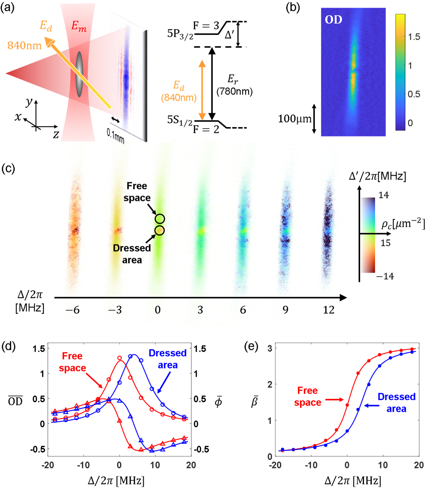
Figure 7: Spectroscopic imaging of a cigar-shaped atomic sample, released from a dipole trap ($E_{m}$), and subjected to a “dimple” $E_{d}$ dressing. (a): The Experimental setup and the level diagram. (b): Typical optical depth image, processed from $\delta I$ averaged over 9 exposures to enhance the display. Here the probe detuning is $\Delta/2\pi=0~{}\rm{MHz}$. (c): $(\Delta^{\prime},\rho_{c})$ in color domain plots. Here $\rho_{c}$ is column density, and $\Delta^{\prime}=-\frac{\Gamma}{2}{\rm tan}\beta$ is the local detuning, both derived from the complex $\varphi_{A}$-data similar to Fig. 4a. (d): ${\rm ROI}-$ averaged $\overline{\rm{OD}}$ and $\overline{\phi}$ spectroscopy. The two Region-Of-Interest (ROI) are marked in (c). The red (blue) curves correspond to region without (with) the $E_{d}$-dressing. The solid lines are according to Eq. (18) with $\xi(s)\propto 1/(1+s)$. (e): The phase-angle spectroscopy of the same data. Similar to Fig. 4(b-i), the fits for the free-space data here give $s_{0}=1.2$ and $\Gamma=2\pi\times 6.0~{}$MHz, within expectations.

References

- Sansonetti et al. [2011] C. J. Sansonetti, C. E. Simien, J. D. Gillaspy, J. N. Tan, S. M. Brewer, R. C. Brown, S. Wu, and J. V. Porto, Absolute transition frequencies and quantum interference in a frequency comb based measurement of the Li6,7 D lines, Physical Review Letters 107, 023001 (2011).
- Lu et al. [2013] Z. Lu, P. Mueller, G. W. F. Drake, and S. C. Pieper, Colloquium : Laser probing of neutron-rich nuclei in light atoms, Rev. Mod. Phys. 85, 1383 (2013).
- Beyer et al. [2017] A. Beyer, L. Maisenbacher, A. Matveev, R. Pohl, K. Khabarova, A. Grinin, T. Lamour, D. C. Yost, T. W. Hänsch, N. Kolachevsky, and T. Udem, The Rydberg constant and proton size from atomic hydrogen, Science 358, 79–85 (2017).
- Fuchs et al. [2018] S. Fuchs, R. Bennett, R. V. Krems, and S. Y. Buhmann, Nonadditivity of Optical and Casimir-Polder Potentials, Phys. Rev. Lett. 121, 83603 (2018).
- Metcalf and van der Straten [1999] H. J. Metcalf and P. van der Straten, Laser Cooling and Trapping( Springer-Verlag) (1999).
- Wynands and Weyers [2005] R. Wynands and S. Weyers, Atomic fountain clocks, Metrologia 42, 64 (2005).
- Ludlow et al. [2015] A. D. Ludlow, M. M. Boyd, and J. Ye, Optical atomic clocks, Review of Modern Physics 87, 637–701 (2015).
- Safronova et al. [2018] M. S. Safronova, D. Budker, D. Demille, D. F. J. Kimball, A. Derevianko, and C. W. Clark, Search for new physics with atoms and molecules, Reviews of Modern Physics 90, 25008 (2018).
- Rengelink et al. [2018] R. J. Rengelink, Y. van der Werf, R. P. Notermans, R. Jannin, K. S. Eikema, M. D. Hoogerland, and W. Vassen, Precision spectroscopy of helium in a magic wavelength optical dipole trap, Nature Physics 14, 1132–1137 (2018), arXiv:1804.06693 .
- Asenbaum et al. [2020] P. Asenbaum, C. Overstreet, M. Kim, J. Curti, and M. A. Kasevich, Atom-Interferometric Test of the Equivalence Principle at the 10-12 Level, Physical Review Letters 125, 191101 (2020), arXiv:2005.11624 .
- Stærkind et al. [2023] H. Stærkind, K. Jensen, J. H. Müller, V. O. Boer, E. T. Petersen, and E. S. Polzik, Precision Measurement of the Excited State Landé g-factor and Diamagnetic Shift of the Cesium D 2 Line , Physical Review X 13, 21036 (2023), arXiv:2208.00077 .
- Zheng et al. [2017] X. Zheng, Y. R. Sun, J. J. Chen, W. Jiang, K. Pachucki, and S. M. Hu, Measurement of the Frequency of the 2 S 3 -2 P 3 Transition of He 4, Physical Review Letters 119, 263002 (2017).
- Brown et al. [2013] R. Brown, S. Wu, J. Porto, C. Sansonetti, C. Simien, S. Brewer, J. Tan, and J. Gillaspy, Quantum interference and light polarization effects in unresolvable atomic lines: Application to a precise measurement of the 6,7Li D 2 lines, Physical Review A 87, 032504 (2013).
- Peyrot et al. [2019] T. Peyrot, N. Šibalić, Y. R. Sortais, A. Browaeys, A. Sargsyan, D. Sarkisyan, I. G. Hughes, and C. S. Adams, Measurement of the atom-surface van der Waals interaction by transmission spectroscopy in a wedged nanocell, Physical Review A 100, 022503 (2019), arXiv:1905.02783 .
- Deist et al. [2022] E. Deist, J. A. Gerber, Y.-H. Lu, J. Zeiher, and D. M. Stamper-Kurn, Superresolution microscopy of optical fields using tweezer-trapped single atoms, Phys. Rev. Lett. 128, 083201 (2022).
- Hilton et al. [2020] A. P. Hilton, A. N. Luiten, and P. S. Light, Light-shift spectroscopy of optically trapped atomic ensembles, New Journal of Physics 22, 033042 (2020), arXiv:1911.02708 .
- Hung et al. [2011] C.-L. Hung, X. Zhang, L.-C. Ha, S.-K. Tung, N. Gemelke, and C. Chin, Extracting density–density correlations from in situ images of atomic quantum gases, New Journal of Physics 13, 075019 (2011).
- Wang et al. [2022] Y. Wang, J. Zhao, X. Huang, L. Qiu, L. Ji, Y. Ma, Y. He, J. P. Sobol, and S. Wu, Imaging Moving Atoms by Holographically Reconstructing the Dragged Slow Light, Physical Review Applied 18, 014065 (2022), arXiv:2105.14832 .
- Zhao et al. [2022] J. Zhao, Y. Wang, X. Huang, and S. Wu, Spectroscopic localization of atomic sample plane for precise digital holography, Optics Express , 18–22 (2022).
- Higbie et al. [2005] J. M. Higbie, L. E. Sadler, S. Inouye, A. P. Chikkatur, S. R. Leslie, K. L. Moore, and V. Savalli, Direct Nondestructive Imaging of Magnetization in a Spin-1 Bose-Einstein Gas, Physical Review Letters 95, 050401 (2005).
- Aljunid et al. [2009] S. A. Aljunid, M. K. Tey, B. Chng, T. Liew, G. Maslennikov, V. Scarani, and C. Kurtsiefer, Phase Shift of a Weak Coherent Beam Induced by a Single Atom, Phys. Rev. Lett. 103, 153601 (2009).
- Kohnen et al. [2011] M. Kohnen, P. G. Petrov, R. A. Nyman1, and E. A. Hinds, Minimally destructive detection of magnetically trapped atoms using frequency-synthesized light, New Journal of Physics 13, 085006 (2011).
- Pototschnig et al. [2011] M. Pototschnig, Y. Chassagneux, J. Hwang, G. Zumofen, A. Renn, and V. Sandoghdar, Controlling the Phase of a Light Beam with a Single Molecule, Physical Review Letters 107, 063001 (2011).
- Fischer et al. [2017] M. Fischer, B. Srivathsan, L. Alber, M. Weber, M. Sondermann, and G. Leuchs, Shifting the phase of a coherent beam with a 174Yb + ion: influence of the scattering cross section, Applied Physics B: Lasers and Optics 123, 48 (2017), arXiv:1609.08335 .
- Zhu et al. [2016] B. Zhu, J. Cooper, J. Ye, and A. M. Rey, Light scattering from dense cold atomic media, Physical Review A 94, 023612 (2016).
- Deb et al. [2020] A. B. Deb, J. Chung, and N. Kjærgaard, Dispersive detection of atomic ensembles in the presence of strong lensing, New Journal of Physics 22, 073017 (2020), arXiv:2002.10618 .
- Agarwal et al. [2024] S. Agarwal, E. Chaparro, D. Barberena, A. P. Orioli, G. Ferioli, S. Pancaldi, I. Ferrier-Barbut, A. Browaeys, and A. M. Rey, Directional superradiance in a driven ultracold atomic gas in free-space, arXiv , 43–47 (2024), arXiv:arXiv:2403.15556v1 .
- Gabor [1972] D. Gabor, Holography, 1948-1971, Proceedings of the IEEE 60, 655 (1972).
- Latychevskaia [2019] T. Latychevskaia, Phase retrieval for digital holography, Journal of the Optical Society of America A 36, 31 (2019).
- Sobol and Wu [2014] J. P. Sobol and S. Wu, Imaging cold atoms with shot-noise and diffraction limited holography, New Journal of Physics 16, 093064 (2014).
- Gabor [1946] D. Gabor, Theory of communication. Part 1: The analysis of information, Journal of the Institution of Electrical Engineers - Part III: Radio and Communication Engineering 93, 429–441 (1946).
- Heller [1975] E. J. Heller, Time-dependent approach to semiclassical dynamics, The Journal of Chemical Physics 62, 1544–1555 (1975).
- Harvey et al. [2015] J. E. Harvey, R. G. Irvin, and R. N. Pfisterer, Modeling physical optics phenomena by complex ray tracing, Optical Engineering 54, 035001 (2015).
- Ashcraft and Douglas [2020] J. N. Ashcraft and E. S. Douglas, An open-source gaussian beamlet decomposition tool for modeling astronomical telescopes, Proc. SPIE 11450,Modeling, Systems Engineering, and Project Management for Astronomy IX, 11450, 1 (2020), arXiv:2106.09162 .
- Braunstein et al. [1996] S. L. Braunstein, C. M. Caves, and G. J. Milburn, Generalized uncertainty relations : Theory , examples , and Lorentz invariance, Annals of Physics 247, 135 (1996), arXiv:9507004v1 [arXiv:quant-ph] .
- Cuche et al. [1999] E. Cuche, F. Bevilacqua, and C. Depeursinge, Digital holography for quantitative phase-contrast imaging, Optics Letters 24, 291 (1999).
- Marquet et al. [2005] P. Marquet, B. Rappaz, P. J. Magistretti, E. Cuche, Y. Emery, T. Colomb, and C. Depeursinge, Digital holographic microscopy: a noninvasive contrast imaging technique allowing quantitative visualization of living cells with subwavelength axial accuracy, Optics Letters 30, 468 (2005).
- Nguyen et al. [2022] T. L. Nguyen, S. Pradeep, R. L. Judson-torres, J. Reed, M. A. Teitell, and T. A. Zangle, Quantitative Phase Imaging : Recent Advances and Expanding Potential in Biomedicine, ACS Nano 16, 11516 (2022).
- foo [a] For the notation conciseness, we may omit the variables, or variables, when expressing the complex and real fields.
- Kadlecek et al. [2001] S. Kadlecek, J. Sebby, R. Newell, and T. G. Walker, Nondestructive spatial heterodyne imaging of cold atoms, Optics Letters 26, 137 (2001).
- Turner et al. [2005] L. D. Turner, K. F. E. M. Domen, and R. E. Scholten, Diffraction-contrast imaging of cold atoms, Physical Review A 72, 031403 (2005).
- Smits et al. [2020] J. Smits, A. P. Mosk, and P. van der Straten, Imaging trapped quantum gases by off-axis holography, Optics Letters 45, 981 (2020), arXiv:1911.09590 .
- Altuntas and Spielman [2021] E. Altuntas and I. B. Spielman, Self-Bayesian Aberration Removal via Constraints for Ultracold Atom Microscopy, Phys. Rev. Res 3, 043087 (2021), arXiv:2108.07106 .
- Yamaguchi and ZHang [1997] I. Yamaguchi and T. ZHang, Phase-shifting digital holography, Optics Letters 22, 1268–1270 (1997).
- Paxman et al. [1992] R. G. Paxman, T. J. Schulz, and J. R. Fienup, Joint estimation of object and aberrations by using phase diversity, Journal of the Optical Society of America A 9, 1072 (1992).
- Ou et al. [2013] X. Ou, R. Horstmeyer, C. Yang, and G. Zheng, Quantitative phase imaging via Fourier ptychographic microscopy, Optics Letters 38, 4845 (2013).
- Perry et al. [2021] A. R. Perry, S. Sugawa, F. Salces-Carcoba, Y. Yue, and I. B. Spielman, Multiple-camera defocus imaging of ultracold atomic gases, Optics Express 29, 17029 (2021), arXiv:2102.08292 .
- Leith and Upatnieks [1962] E. N. Leith and J. Upatnieks, Reconstructed Wavefronts and Communication Theory*, Journal of the Optical Society of America 52, 1123 (1962).
- Gao et al. [2013] P. Gao, G. Pedrini, and W. Osten, Structured illumination for resolution enhancement and autofocusing in digital holographic microscopy, Optics Letters 11, 090901 (2013).
- Zuo et al. [2020] C. Zuo, J. Li, J. Sun, Y. Fan, J. Zhang, L. Lu, R. Zhang, B. Wang, L. Huang, and Q. Chen, Transport of intensity equation: a tutorial, Optics and Lasers in Engineering 135, 106187 (2020).
- foo [b] The highly sensitive relation between the apparent and at the sample plane is exploited itself for holographic imaging of cold atoms, as in ref. [41] and more generally discussed in ref. [43]. Here, since we plan is to measure and , their relation cannot be assumed as a prior knowledge in general.
- Ilhan et al. [2013] H. A. Ilhan, M. Doğar, and M. Özcan, in Practical Holography XXVII: Materials and Applications, Vol. 8644 (SPIE, 2013) pp. 77–87.
- Brady et al. [2009] D. J. Brady, K. Choi, D. L. Marks, R. Horisaki, and S. Lim, Compressive Holography, Opt. Express 17, 13040 (2009).
- Zhang et al. [2017] Y. Zhang, H. Wang, Y. Wu, M. Tamamitsu, and A. Ozcan, Edge sparsity criterion for robust holographic autofocusing, Optics Letters 42, 3824 (2017).
- Fan et al. [2017] X. Fan, J. J. Healy, and B. M. Hennelly, Investigation of sparsity metrics for autofocusing in digital holographic microscopy, Opt. Eng. 56, 053112 (2017).
- Wu et al. [2018] Y. Wu, Y. Rivenson, Y. Zhang, Z. Wei, H. Günaydin, X. Lin, and A. Ozcan, Extended depth-of-field in holographic imaging using deep-learning-based autofocusing and phase recovery, Optica 5, 704 (2018).
- Redding et al. [2012] B. Redding, M. A. Choma, and H. Cao, Speckle-free laser imaging using random laser illumination, Nature Photonics 6, 355 (2012).
- Koren et al. [1993] G. Koren, F. Polack, and D. Joyeux, Iterative algorithms for twin-image elimination in in-line holography using finite-support constraints, Journal of the Optical Society of America A 10, 423 (1993).
- Isikman et al. [2011] S. O. Isikman, W. Bishara, S. Mavandadi, F. W. Yu, S. Feng, R. Lau, and A. Ozcan, Lens-free optical tomographic microscope with a large imaging volume on a chip, Proceedings of the National Academy of Sciences of the United States of America 108, 7296 (2011).
- Latychevskaia and Fink [2007] T. Latychevskaia and H.-w. Fink, Solution to the Twin Image Problem in Holography, Phys. Rev. Lett. 98, 233901 (2007).
- Marti et al. [2018] G. E. Marti, R. B. Hutson, A. Goban, S. L. Campbell, N. Poli, and J. Ye, Imaging Optical Frequencies with 100 muHz Precision and 1 . 1 mu m Resolution, Physical Review Letters 120, 103201 (2018).
- Li et al. [2020] R. Li, Y. Wu, Y. Rui, B. Li, Y. Jiang, L. Ma, and H. Wu, Absolute Frequency Measurement of Li 6 D Lines with khz-Level Uncertainty, Physical Review Letters 124, 063002 (2020).
- Chomaz et al. [2012] L. Chomaz, L. Corman, T. Yefsah, R. Desbuquois, and J. Dalibard, Absorption imaging of a quasi-two-dimensional gas: a multiple scattering analysis, New Journal of Physics 14, 055001 (2012).
- Kuhr [2016] S. Kuhr, Special Topic : Cold Atoms Quantum-gas microscopes : a new tool for cold-atom quantum simulators, Nature Science Review 3, 170–172 (2016).
- Zheng et al. [2013a] G. Zheng, R. Horstmeyer, and C. Yang, Wide-field, high-resolution Fourier ptychographic microscopy, Nature Photonics 7, 739 (2013a).
- Zheng et al. [2013b] G. Zheng, X. Ou, R. Horstmeyer, and C. Yang, Characterization of spatially varying aberrations for wide field-of-view microscopy, Optics Express 21, 15131 (2013b).
- Park et al. [2021a] K. Park, T. Kong, T. D. Yang, and Y. Choi, Measurement of multiple phase maps for wide-area aberration correction by switchable optical configuration, Optics Express 29, 41894 (2021a).
- Sobol [2015] J. P. Sobol, Imaging cold atoms with shot-noise and diffraction limited holography, Ph.D. thesis, Swansea University (2015).
- Yang et al. [1994] G.-z. Yang, B.-z. Dong, B.-y. Gu, J.-y. Zhuang, and O. K. Ersoy, Gerchberg–Saxton and Yang–Gu algorithms for phase retrieval in a nonunitary transform system: a comparison, Applied Optics 33, 209 (1994).
- Meppelink et al. [2010] R. Meppelink, R. A. Rozendaal, S. B. Koller, J. M. Vogels, and P. V. D. Straten, Thermodynamics of Bose-Einstein-condensed clouds using phase-contrast imaging, Physical Review A 81, 053632 (2010).
- Reinaudi et al. [2007] G. Reinaudi, T. Lahaye, Z. Wang, and D. Guéry-Odelin, Strong saturation absorption imaging of dense clouds of ultracold atoms, Optics Letters 32, 3143 (2007), arXiv:0707.2930 .
- [72] D. A. Steck, Rubidium 87 D Line Data, http://steck.us/alkalidata (revision 2.2.1, 21 November 2019). .
- Alt [2002] W. Alt, An objective lens for efficient fluorescence detection of single atoms, Optik (Jena) 113, 142–144 (2002), arXiv:0108058 [physics] .
- Li et al. [2018] X. Li, F. Zhou, M. Ke, P. Xu, X.-D. He, J. Wang, and M.-S. Zhan, High-resolution ex vacuo objective for cold atom experiments, Applied Optics 57, 7584 (2018).
- Bruce et al. [2017] G. D. Bruce, E. Haller, B. Peaudecerf, D. A. Cotta, M. Andia, S. Wu, M. Y. Johnson, B. W. Lovett, and S. Kuhr, Sub-Doppler laser cooling of 40K with Raman gray molasses on the D2 line, Journal of Physics B: Atomic, Molecular and Optical Physics 50, 095002 (2017), arXiv:1612.04583 .
- foo [c] By comparing the shot-to-shot data between different samples, noticeable correlations can be found at a level consistent with the frequency noise of our saturation-spectrum-locked cateye laser (Moglabs CEL) at 100 kHz level. The relative phase-angle variations are close to the photon-shot-noise limit set by Eq. (9).
- Bachelard et al. [2016] R. Bachelard, N. Piovella, W. Guerin, and R. Kaiser, Collective effects in the radiation pressure force, Phys. Rev. A 94, 033836 (2016).
- Bons et al. [2016] P. C. Bons, R. De Haas, D. De Jong, A. Groot, and P. Van Der Straten, Quantum Enhancement of the Index of Refraction in a Bose-Einstein Condensate, Phys. Rev. Lett. 116, 173602 (2016).
- Gross and Bloch [2017] C. Gross and I. Bloch, Quantum simulations with ultracold atoms in optical lattices., Science 357, 995–1001 (2017).
- Bakr et al. [2009] W. S. Bakr, J. I. Gillen, A. Peng, S. Fölling, and M. Greiner, A quantum gas microscope for detecting single atoms in a Hubbard-regime optical lattice, Nature 462, 74–77 (2009), arXiv:0908.0174 .
- Sherson et al. [2010] J. F. Sherson, C. Weitenberg, M. Endres, M. Cheneau, I. Bloch, and S. Kuhr, Single-Atom Resolved Fluorescence Imaging of an Atomic Mott Insulator, Nature 467, 68 (2010), arXiv:arXiv:1006.3799v2 .
- Okuno et al. [2020] D. Okuno, Y. Amano, K. Enomoto, N. Takei, and Y. Takahashi, Schemes for nondestructive quantum gas microscopy of single atoms in an optical lattice, New J. Phys. 22, 013041 (2020).
- Nelson et al. [2007] K. D. Nelson, X. Li, and D. S. Weiss, Imaging single atoms in a three-dimensional array, Nature Physics 3, 556 (2007).
- Barredo et al. [2018] D. Barredo, V. Lienhard, S. de Léséleuc, T. Lahaye, and A. Browaeys, Synthetic three-dimensional atomic structures assembled atom by atom, Nature 561, 79–82 (2018), arXiv:1712.02727 .
- Spielman et al. [2007] I. B. Spielman, W. D. Phillips, and J. V. Porto, Mott-Insulator Transition in a Two-Dimensional Atomic Bose Gas, Phys. Rev. Lett. 98, 080404 (2007).
- Greenbaum et al. [2012] A. Greenbaum, W. Luo, T. W. Su, Z. Göröcs, L. Xue, S. O. Isikman, A. F. Coskun, O. Mudanyali, and A. Ozcan, Imaging without lenses: Achievements and remaining challenges of wide-field on-chip microscopy, Nat. Methods 9, 889 (2012).
- De Haan et al. [2020] K. De Haan, Y. Rivenson, Y. Wu, and A. Ozcan, Deep-Learning-Based Image Reconstruction and Enhancement in Optical Microscopy, Proc. IEEE 108, 2949575 (2020).
- Park et al. [2021b] J. Park, D. J. Brady, G. Zheng, L. Tian, and L. Gao, Review of bio-optical imaging systems with a high space-bandwidth product, Adv. Photonics 3, 044001 (2021b).
- Kong et al. [2016] X. Kong, A. Markmann, and V. S. Batista, Time-Sliced Thawed Gaussian Propagation Method for Simulations of Quantum Dynamics, Journal of Physical Chemistry A 120, 3260–3269 (2016).
- Worku and Gross [2020] N. G. Worku and H. Gross, Gaussian pulsed beam decomposition for propagation of ultrashort pulses through optical systems, Journal of the Optical Society of America A 37, 98 (2020).
- Legrand et al. [2024] T. Legrand, F. R. Winkelmann, W. Alt, D. Meschede, A. Alberti, and C. A. Weidner, Three-dimensional imaging of single atoms in an optical lattice via helical point-spread-function engineering, Physical Review A 109, 033304 (2024), arXiv:2312.05341 .
- Diego et al. [2023] S. Diego, S. Diego, M. E. Mossman, R. A. Corbin, M. M. Forbes, and P. Engels, Atom Interferometric Imaging of Differential Potentials Using an Atom Laser, Physical Review Letters 130, 263402 (2023).
- Ji et al. [2023] L. Ji, Y. He, Q. Cai, Z. Fang, Y. Wang, L. Qiu, L. Zhou, S. Wu, and S. Grava, Superradiant Detection of Microscopic Optical Dipolar Interactions, Phys. Rev. Lett. 131, 253602 (2023).
- Rui et al. [2020] J. Rui, D. Wei, A. Rubio-Abadal, S. Hollerith, J. Zeiher, D. M. Stamper-Kurn, C. Gross, and I. Bloch, A subradiant optical mirror formed by a single structured atomic layer, Nature 583, 369–374 (2020), arXiv:2001.00795 .
- Deb and Kjærgaard [2021] A. B. Deb and N. Kjærgaard, Observation of Pauli blocking in light scattering from quantum degenerate fermions, Science (80-. ). 374, 972–975 (2021).
- Lu et al. [2022] Y. K. Lu, Y. Margalit, and W. Ketterle, Bosonic stimulation of atom–light scattering in an ultracold gas, Nature Physics 19, 210–214 (2022).
- Srakaew et al. [2023] K. Srakaew, P. Weckesser, S. Hollerith, D. Wei, D. Adler, I. Bloch, and J. Zeiher, A subwavelength atomic array switched by a single Rydberg atom, Nature Physics 10, 1038 (2023), 2207.09383 .
- Lye et al. [2003] J. E. Lye, J. J. Hope, and J. D. Close, Nondestructive dynamic detectors for Bose-Einstein condensates, Phys. Rev. A 67, 043609 (2003).
- Miao et al. [1999] J. Miao, P. Charalambous, J. Kirz, and D. Sayre, Extending the methodology of X-ray crystallography to non-crystalline specimens, Nature 400, 342 (1999).
- Babiker et al. [2013] M. Babiker, D. L. Andrews, V. E. Lembessis, M. Hamamda, P. Pillet, Y. Yin, and Y. Xia, Sisyphus cooling in a continuously loaded trap, New Journal of Physics 15, 093012 (2013).
- La Rooij et al. [2023] A. La Rooij, C. Ulm, E. Haller, and S. Kuhr, A comparative study of deconvolution techniques for quantum-gas microscope images, New Journal of Physics 25, 083036 (2023), arXiv:2207.08663 .
- Castin [2001] Y. Castin, in COHERENT ATOMIC MATTER WAVES, LES HOUCHES SUMMER SCHOOL SESSION, Vol. 72, edited by R. Kaiser, C. Westbrook, and F. David (NATO, Adv Study Inst, 2001) pp. 5–136.
- Kingma and Ba [2015] D. P. Kingma and J. L. Ba, Adam: A method for stochastic optimization, 3rd International Conference on Learning Representations, ICLR 2015 - Conference Track Proceedings , 1–15 (2015), arXiv:1412.6980 .