Multi-Objective Optimization-based Transmit Beamforming for Multi-Target and Multi-User MIMO-ISAC Systems

Abstract

Integrated sensing and communication (ISAC) is an enabling technology for the sixth-generation mobile communications, which equips the wireless communication networks with sensing capabilities. In this paper, we investigate transmit beamforming design for multiple-input and multiple-output (MIMO)-ISAC systems in scenarios with multiple radar targets and communication users. A general form of multi-target sensing mutual information (MI) is derived, along with its upper bound, which can be interpreted as the sum of individual single-target sensing MI. Additionally, this upper bound can be achieved by suppressing the cross-correlation among reflected signals from different targets, which aligns with the principles of adaptive MIMO radar. Then, we propose a multi-objective optimization framework based on the signal-to-interference-plus-noise ratio of each user and the tight upper bound of sensing MI, introducing the Pareto boundary to characterize the achievable communication-sensing performance boundary of the proposed ISAC system. To achieve the Pareto boundary, the max-min system utility function method is employed, while considering the fairness between communication users and radar targets. Subsequently, the bisection search method is employed to find a specific Pareto optimal solution by solving a series of convex feasible problems. Finally, simulation results validate that the proposed method achieves a better tradeoff between multi-user communication and multi-target sensing performance. Additionally, utilizing the tight upper bound of sensing MI as a performance metric can enhance the multi-target resolution capability and angle estimation accuracy.

I Introduction

The next-generation wireless networks (6G and 5G-beyond) have been envisioned as a vital enabler for numerous emerging applications, such as autonomous vehicles, smart cities, and the Internet of Things [1, 2]. The challenging problem is to satisfy the requirements of these applications for efficient communication and high-accuracy sensing, which motivates the development of frameworks for communication-sensing integration. As such, integrated sensing and communications (ISAC) has been proposed as an appealing technology and has attracted great research interests recently[2, 3, 4, 5, 6]. In particular, ISAC can significantly enhance the spectral efficiency and reduce the hardware software complexity by sharing the hardware platform and the resources in spatial, temporal as well as frequency domains for both communication and sensing [7, 8, 3].

The multiple-input and multiple-output (MIMO) technique plays a significant role in ISAC systems, which enables spatial multiplexing, diversity, and beamforming, leading to higher data rates, improved link reliability, enhanced spatial resolution, and accurate target parameter estimation[9, 10]. However, the inherent difference between communication and sensing leads to compromised performance, posing challenges for MIMO-ISAC systems. Therefore, the key issue is to design effective transmit beamforming strategies that can flexibly balance the performance of both functionalities while catering to the diverse requirements in practical scenarios. Numerous studies have investigated the joint optimization of transmit beamforming by considering both communication and sensing performance metrics [11, 12, 13, 14, 15, 16, 17, 18, 19, 20, 21]. The work of [14] optimized the transmit beamforming by maximizing the peak sidelobe level of radar while ensuring given signal-to-interference-plus-noise ratio (SINR) threshold levels for the users. Furthermore, the studies conducted in [13, 12] decomposed the transmit waveform into radar and communication waveform, and optimize the beamformers for each waveform to satisfy the respective performance requirements for sensing and communication. Addtionally, in the context of specific sensing tasks such as target estimation and tracking, some literature employs the Cramér-Rao bound (CRB) as a performance metric to evaluate the estimation performance of target parameters [18, 19, 20]. In [18], the authors minimized the CRB on parameter estimates for a single target while ensuring the pre-defined communication SINR threshold for each downlink user. Then, the authors in [20] minimized the multi-target estimation CRB, subject to the minimum communication requirement. However, the lower bound for estimation accuracy provided by CRB may be not tight at low signal-to-noise ratio (SNR), and its complex and non-convex mathematical nature always results in a more challenging optimization problem.

As a comparison, mutual information (MI) is also a commonly used sensing performance metric, which provides accurate estimation and classification capabilities in a more concise form[22, 8]. In [23], the authors demonstrated that the optimal waveform designed by maximizing sensing MI enables efficient coexistence of MIMO radar and communication systems occupying the same spectrum. In [24], the authors showed that under the assumption of Gaussian distributed target response, maximizing MI and maximizing minimum mean square error (MMSE) lead to the same optimal waveform solution. In [15], the emphasis on the accuracy of entire sensing channel vectors with sensing MI enhances overall sensing performance beyond the focus on specific parameter-associated partial channels with the CRB. The authors in [25] showed that maximizing sensing MI through the waveform design improved the target detection and feature extraction performance. Besides, the similarity between the communication and sensing MI expressions also facilitates the efficient tradeoff between the two functionalities through weighted sum optimization[16, 26]. The authors in [16] optimized a weighted sum of communication and sensing MI to improve the balanced performance of both functionalities. In [27], the authors established a relationship between sensing MI and the rate-distortion theory, imparting operational estimation theoretic meaning to MI-based methods. Furthermore, [28] demonstrated that MI-based beamforming design can effectively suppress echo interference from scatters in the surrounding environment.

Simultaneously supporting multi-user communication and multi-target sensing in practical scenarios poses a critical challenge for MIMO-ISAC systems[20, 14]. Such scenarios are inherently complex due to the diverse performance requirements for both communication and sensing. Moreover, they involve multiple intrinsic tradeoffs, such as the performance tradeoffs among multiple communication users, multiple sensing targets, and between communication and sensing. Therefore, it is essential to develop a beamforming method that can flexibly balance multi-user communication and multi-target sensing performance based on their respective priorities. Given its advantages in enhancing target detection, estimation, and classification performance in a concise manner, sensing MI serves as a more suitable performance metric for multi-target sensing, as mentioned before[25, 15, 26, 27, 28, 16, 17]. However, existing research based on sensing MI still has some limitations. Firstly, sensing MI in current studies offers a general overview of the sensing channel containing the multi-target information, but lacks a clear and detailed characterization of multi-target sensing performance and the relationships between targets. Secondly, the lack of precise depiction of achievable performance boundaries for communication and sensing hinders the attainment of optimal performance tradeoffs. Furthermore, the absence of fairness consideration between users and targets poses limitations on meeting diverse and specific requirements, thereby impeding the flexibility of beamforming designs.

To address these limitations, we propose a novel transmit beamforming approach for multi-user multi-target MIMO-ISAC systems based on the sensing MI and communication SINRs. We consider a scenario where the base station (BS) communicates with multiple downlink users while sensing multiple targets simultaneously. To fully exploit the degrees of freedom (DoF)s provided by MIMO to meet the performance requirements of both multi-user communication and multi-target sensing, we synthesize communication and radar signals, and then jointly design their respective transmit beamforming[13, 12, 18]. Then, we derive a general expression for sensing MI and its tight upper bound to explore the structural features of maximum sensing MI. We find that maximizing the MI upper bound under zero-forced cross-correlation constraints aligns with the principles of adaptive MIMO radar technique[29]. Therefore, we utilize the constrained upper bound of sensing MI as the performance metric for multi-target sensing, each user’s SINR as the communication performance metric, and construct a multi-objective optimization problem (MOOP) to comprehensively investigate the tradeoff in communication-sensing performance. To efficiently solve the MOOP, we define the achievable performance region and its Pareto boundary. Then, we formulate a max-min utility optimization problem to obtain a specific Pareto solution for the MOOP, and utilize the properties of the achievable performance region to prove that the optimal solution of this max-min problem lies on the Pareto boundary. Finally, a bisection search method is employed to find the Pareto optimal solution for a specific set of communication-sensing weights. The main contributions of this paper are summarized as follows:

• We derive a novel general form of multi-target sensing MI and alongside a tight upper bound that satisfies zero-forced cross-correlation constraints. Furthermore, by suppressing the cross-correlation among signals reflected from different targets, not only can sensing MI reach its maximum, but the signals can also be considered independent of each other, which benefits target detection and tracking. Remarkably, we find that the upper bound of sensing MI can be viewed as the sum of single-target sensing MI, resembling a concise form similar to communication sum-rate and simplifying subsequent optimization processes.

• To comprehensively investigate the tradeoff in communication and sensing performance, we formulate a MOOP to simultaneously optimize communication SINRs and sensing MI. Then, we introduce the Pareto boundary of the MOOP to characterize the achievable performance boundary of the proposed ISAC system. To obtain a specific set of Pareto solutions, a max-min utility function method is employed, which can be solved through a bisection search algorithm. This method provides a flexible tradeoff between multi-target sensing and multi-user communication performance, while meeting specific sensing and communication requirements and their respective priorities.

• Finally, numerical simulations demonstrate the following: i) The necessity of transmitting additional radar signals to provide sufficient DoFs for effectively resolving multiple targets, particularly when the number of targets surpasses the number of users. ii) The adoption of the constrained sensing MI upper bound as the performance metric for multi-target sensing offers an enhanced tradeoff between sensing and communication performance. Moreover, it also significantly improves resolution for closely located multiple targets and enhances accuracy in angle estimation.

The rest of this paper is organized as follows. Section II introduces the system model along with the performance metric for multi-user communications. Section III derives the sensing MI and its tight upper bound for multi-target sensing. Section IV investigates the multi-objective optimization for ISAC beamforming, where we employ a max-min utility function method to solve the MOOP. Simulation results are presented in Section V. Finally, we provide concluding remarks in Section VI.

Notations: Boldface lowercase and uppercase letters denote vectors and matrices, respectively. The set of complex number is $\mathbb{C}$. The transpose, conjugate transpose, conjugate, inverse and pseudo-inverse operation is denoted by $(\cdot)^{T}$, $(\cdot)^{H}$, $(\cdot)^{*}$ , $(\cdot)^{-1}$ and $(\cdot)^{\dagger}$, respectively. The expected value of a random argument is denoted by $\mathbb{E}(\cdot)$. We let $\otimes$ denote the Kronecker product, and let $\mathbf{I}_{M}$ denote the $M$-dimensional identity matrix. The curled inequality symbol $\succeq$ is utilized to denote the generalized matrix inequality, i.e., $\mathbf{A}\succeq\mathbf{0}$ means that $\mathbf{A}$ is positive semi-definite matrix. The symbols $\text{det}(\cdot)$ and $\text{tr}(\cdot)$ denote the determinant and trace of a matrix, respectively.

II System Model

Figure 1: Illustration of the ISAC scenario where the BS serves $C$ downlink communication users while detecting $K$ targets.

We consider a colocated ISAC system as shown in Fig. 1, where the BS is equipped with ${{N}_{t}}$ transmit antennas and ${N}_{r}$ receive antennas as uniform linear arrays (ULAs). The BS aims to serve $C$ downlink single-antenna users while detecting $K$ targets. The set of communication users is indexed by $\mathcal{C}=\{1,2,\ldots,C\}$. To achieve the satisfactory performance of communication and radar sensing, we exploit the maximum DoFs provided by MIMO and transmit ${M}$ additional probing streams. The transmit signal is a sum of precoded communication signals and radar probing signals [13, 18, 12], i.e.,

$$\mathbf{X}={{\mathbf{W}}_{c}}{{\mathbf{S}}_{c}}+{{\mathbf{W}}_{r}}{{\mathbf{S}}_{r}},$$ (1)

where $\mathbf{X}\in\mathbb{C}^{N_{t}\times L}$ is the transmit signal matrix with $L>{N}_{t}$ being the length of the signals. The $i$th data stream of the communication is denoted by ${\mathbf{s}}_{i}$, $\forall i\in\mathcal{C}$, and ${{\mathbf{S}}_{c}}={{\left[\mathbf{s}_{1}^{T},\ldots,\mathbf{s}_{C}^{T}\right]}^{T}}\in{{\mathbb{C}}^{{{C}}\times{{L}}}}$ contains $C$ data streams intended for the ${C}$ users. Similarly, the $m$-th probing stream of radar sensing is denoted by ${\mathbf{s}}_{C+m}$, $m\in\left\{1,2,\cdots,M\right\}$, and ${{\mathbf{S}}_{r}}={{\left[\mathbf{s}_{{C}+1}^{T},\ldots,\mathbf{s}_{{C}+M}^{T}\right]}^{T}}\in{{\mathbb{C}}^{{{M}}\times{{L}}}}$ contains $M$ individual probing streams with $M<N_{t}-C$[18]. The matrices ${{\mathbf{W}}_{c}}=\left[{{\mathbf{w}}_{1}},\ldots,{{\mathbf{w}}_{{{C}}}}\right]\in{{\mathbb{C}}^{{{N}_{t}}\times{{C}}}}$ and ${{\mathbf{W}}_{r}}=\left[{{\mathbf{w}}_{{C}+1}},\ldots,{{\mathbf{w}}_{{C}+M}}\right]\in{{\mathbb{C}}^{{{N}_{t}}\times{M}}}$ contain the transmit beamforming vectors for the data streams and the probing streams, respectively.

We assume that both the communication signals and radar probing signals are wide-sense stationary stochastic processes with zero mean and unit power[13]. The communication data signals for different users are uncorrelated, so $\frac{1}{L}\mathbb{E}\left[{{\mathbf{S}}_{c}}\mathbf{S}_{c}^{H}\right]={{\mathbf{I}}_{{{C}}}}$. The radar probing signals are pseudorandom sequences with zero mean and unit variance, and are uncorrelated with each other[30], i.e., $\frac{1}{L}\mathbb{E}\left[{{\mathbf{S}}_{r}}\mathbf{S}_{r}^{H}\right]={{\mathbf{I}}_{{{M}}}}$. The communication signals and radar probing signals are assumed to be uncorrelated, namely $\mathbb{E}\left[{{\mathbf{S}}_{c}}\mathbf{S}_{r}^{H}\right]={{\mathbf{0}}}$. Then, we can derive the covariance matrix of the transmit signal, given by

$$\mathbf{R}_{X}=\frac{1}{L}\mathbb{E}\left[\mathbf{X}{{\mathbf{X}}^{H}}\right]=\sum\limits_{n=1}^{C+M}{{{\mathbf{w}}_{n}}\mathbf{w}_{n}^{H}},$$ (2)

In the following, we describe the received signal model and the performance metric for multi-user communications in Subsection II-A. Subsequently, we present the receive signal model for radar sensing at the BS in Subsection II-B.

II-A Multi-User Communication Model

For downlink communications, the signal received at the $i$-th user is expressed as

$${{\mathbf{y}}_{i}} =\mathbf{h}_{i}^{H}\mathbf{X}+{{\mathbf{z}}_{i}},$$ (3)

where ${{\mathbf{h}}_{i}}\in{{\mathbb{C}}^{{{N}_{t}}\times 1}}$ is the channel matrix between the BS and the $i$-th user, and ${{\mathbf{z}}_{i}}\sim\mathcal{C}\mathcal{N}(0,{\sigma_{i}^{2}\mathbf{I}_{L}})$ is a complex additive white Gaussian noise (AWGN) vector with zero mean and covariance $\sigma_{i}^{2}\mathbf{I}_{L}$.

Since the communication users have no prior information about the probing streams, the users suffer from the interference caused by the probing streams and the multi-user interference[13, 18]. Specifically, the received signal (3) can be rewritten as

$${{\mathbf{y}}_{i}}=\mathbf{h}_{i}^{H}{{\mathbf{w}}_{i}}{{\mathbf{s}}_{i}}+\!\!\!\sum\limits_{j=1,j\neq i}^{C}{\mathbf{h}_{i}^{H}{{\mathbf{w}}_{j}}}{{\mathbf{s}}_{j}}+\!\!\!\sum\limits_{j=C+1}^{C+M}{\mathbf{h}_{i}^{H}{{\mathbf{w}}_{j}}}{{\mathbf{s}}_{j}}+{{\mathbf{z}}_{i}},\forall i\in\mathcal{C},$$ (4)

where the initial term is the useful signal, while the second term denotes the interference caused by the other communication users. The third term indicates the interference originating from the radar probing signals. Thus, the SINR of the $i$-th user is

$${{\gamma}_{i}}=\frac{{{\left|\mathbf{h}_{i}^{H}{{\mathbf{w}}_{i}}\right|}^{2}}}{\sum_{j=1,j\neq i}^{C}{{{\left|\mathbf{h}_{i}^{H}{{\mathbf{w}}_{j}}\right|}^{2}}}+\sum_{j=C+1}^{C+M}{{{\left|\mathbf{h}_{i}^{H}{{\mathbf{w}}_{j}}\right|}^{2}}}+\sigma_{i}^{2}}.$$ (5)

The overall performance of the multi-user multiple-input and multiple-output (MU-MIMO) communication is evaluated by the average rate, which is given by [31]

$${{r}_{c}}=\frac{1}{C}\left(\sum\limits_{i=1}^{C}{\log\left(1+{{\gamma}_{i}}\right)}\right).$$ (6)

II-B Radar Sensing Model

The BS uses the reflected echoes to recover the parameters of the targets. In this paper, we focus on beamforming in the spatial domain. For brevity, the sensing targets are modeled to be stationary, and are located at the same range resolution as assumed in [11, 32, 18]. With these assumptions, the target response matrix is expressed as the superposition of the response of the individual target [33], i.e.,

$$\mathbf{G}=\sum\limits_{k=1}^{K}{{{\beta}_{k}}\text{ }\mathbf{b}\left({{\theta}_{k}}\right)}\text{ }{{\mathbf{a}}^{H}}\left({{\theta}_{k}}\right),$$ (7)

where $\mathbf{a}\left(\theta_{k}\right)={{[1,{{e}^{j\frac{2\pi}{\lambda}{d}\sin\left(\theta_{k}\right)}},\ldots,{{e}^{j\frac{2\pi}{\lambda}\left({{N}_{t}}-1\right){d}\sin\left(\theta_{k}\right)}}]}^{T}}\in{{\mathbb{C}}^{{{N}_{t}}\times 1}}$ and $\mathbf{b}\left(\theta_{k}\right)=[1,{{e}^{j\frac{2\pi}{\lambda}{d}\sin\left(\theta_{k}\right)}},\ldots,$ ${{{e}^{j\frac{2\pi}{\lambda}\left({{N}_{r}}-1\right){d}\sin\left(\theta_{k}\right)}}]}^{T}\in{{\mathbb{C}}^{{{N}_{r}}\times 1}}$ are the corresponding transmit and receive steering vectors of the echo with the direction at $\theta_{k}$, respectively. In general, the target can be modeled as being composed of an infinite number of random, isotropic and independent scatterers over the area of interest, and the complex gain of each scatterer can be modeled as a zero-mean and white complex random variable [34]. Together with the fact that the incident angles between different targets are independently distributed [35], the complex coefficients of different targets can be assumed to be independently Gaussian distributed, i.e., $\beta_{k}\sim\mathcal{CN}\left(0,{\sigma}_{k}^{2}\right),\forall k$ [36].

The distance of adjacent antenna elements is denoted by $d$, and $\lambda$ denotes the wavelength. Thus, the signal received at the BS is given by

$${{\mathbf{Y}}_{r}}=\mathbf{GX}+{{\mathbf{Z}}_{r}},$$ (8)

where ${{\mathbf{Z}}_{r}}\in{{\mathbb{C}}^{{{N}_{r}}\times L}}$ is a complex AWGN matrix with zero mean and covariance $\sigma_{r}^{2}\mathbf{I}_{L}$.

Upon vectorizing (8), the received signal is recast as

$${{\mathbf{\tilde{y}}}_{r}}=\mathbf{\tilde{X}\tilde{g}}+{{\mathbf{\tilde{z}}}_{r}},$$ (9)

where ${{\mathbf{\tilde{y}}}_{r}}\triangleq\text{vec}({{\mathbf{Y}}_{r}})$, $\mathbf{\tilde{X}}\triangleq({{\mathbf{X}}^{T}}\otimes{{\mathbf{I}}_{{{N}_{r}}}})$, $\mathbf{\tilde{g}}\triangleq\text{vec}(\mathbf{G})$, and ${{\mathbf{\tilde{z}}}_{r}}\triangleq\text{vec}({{\mathbf{Z}}_{r}})$. Let ${\mathbf{R}}_{G}=\mathbb{E}[\mathbf{\tilde{g}}{{{\mathbf{\tilde{g}}}}^{H}}]$ be the spatial correlation matrix of $\mathbf{G}$, and ${\mathbf{R}}_{Z}=\mathbb{E}[{{\mathbf{\tilde{z}}}_{r}}{{{\mathbf{\tilde{z}}}_{r}}^{H}}]$ be the covariance matrix of ${{\mathbf{\tilde{z}}}_{r}}$. To facilitate the derivation, we assume $\mathbf{\tilde{g}}\sim\mathcal{C}\mathcal{N}(\mathbf{0},{{\mathbf{R}}_{G}})$, which is consistent with the classic literature on radar MI[22, 37, 23]. Then, we have ${{\mathbf{\tilde{z}}}_{r}}\sim\mathcal{C}\mathcal{N}(\mathbf{0},{{\mathbf{R}}_{Z}})$ and ${{\mathbf{\tilde{y}}}_{r}}\sim\mathcal{C}\mathcal{N}(\mathbf{0},\mathbf{\tilde{X}}{{\mathbf{R}}_{G}}{{{\mathbf{\tilde{X}}}}^{H}}+{{\mathbf{R}}_{Z}})$. The covariance matrix ${\mathbf{R}}_{G}$ is given by

$${\mathbf{R}}_{G}\!=\!\mathbb{E}\left[\mathbf{\tilde{g}}{{{\mathbf{\tilde{g}}}}^{H}}\right]\!\overset{\left(a\right)}{=}\!\sum_{k=1}^{K}{\sigma_{k}^{2}\left({{\mathbf{a}}^{*}}\!\!\left({{\theta}_{k}}\right)\!\otimes\!\mathbf{b}\left({{\theta}_{k}}\right)\right){{\left({{\mathbf{a}}^{*}}\!\!\left({{\theta}_{k}}\right)\!\otimes\!\mathbf{b}\left({{\theta}_{k}}\right)\right)}^{H}}},$$ (10)

where $\left(a\right)$ follows $\text{vec}(\mathbf{\mathbf{b}\mathbf{a}^{H}})=({{\mathbf{a}}^{*}}\otimes\mathbf{b})$.

To demonstrate the necessity of transmitting additional radar signals, we consider a scenario where only $C$ communication signals are transmitted, i.e., $\mathbf{X}={{\mathbf{W}}_{c}}{{\mathbf{S}}_{c}}$. In this case, the number of DoFs for transmit bemaforming design is limited by the number of communication users due to the fact that $\text{rank}(\mathbf{R}_{X})=C$. However, when there exists $K$ targets with $K>C$, the number of available DoFs is insufficient to for accurate estimation of the targets using angle estimation techniques such as multiple signal classification (MUSIC) and Capon[29]. Consequently, this leads to an inevitable degradation in the performance of multi-target sensing due to the lack of radar DoFs[18]. Therefore, it is imperative to transmit additional radar signals in scenarios with a large number of targets. The detailed analysis is provided in Section V.

III Mutual Information for Radar Sensing

In order to characterize the performance of multi-target sensing, we introduce the sensing MI which can be employed to measure how much environmental information can be observed in the BS[22]. The sensing MI is generally defined as the conditional MI between the sensing channel $\mathbf{\tilde{g}}$ and the received signal ${{{\mathbf{\tilde{y}}}}_{r}}$ with the given transmit signal[16]. Following [38], we obtain the general expression of sensing MI as

$$I\left({{{\mathbf{\tilde{y}}}}_{r}};\mathbf{\tilde{g}}\left|{\mathbf{\tilde{X}}}\right.\right) =\log\left[\det\!\left(\mathbf{\tilde{X}}{{\mathbf{R}}_{G}}{{{\mathbf{\tilde{X}}}}^{H}}+{{\mathbf{R}}_{Z}}\right)\right]\!-\!\log\left[\det\left({{\mathbf{R}}_{Z}}\right)\right]$$ (11)

$$=\log\left[\det\left(\mathbf{I}+\mathbf{\tilde{X}}{{\mathbf{R}}_{G}}{{{\mathbf{\tilde{X}}}}^{H}}\mathbf{R}_{Z}^{-1}\right)\right]$$

$$\overset{\left(a\right)}{=}\log\left[\det\left(\mathbf{I}+\frac{1}{\sigma_{r}^{2}}{{\mathbf{R}}_{G}}{{{\mathbf{\tilde{X}}}}^{H}}\mathbf{\tilde{X}}\right)\right],$$

where $\mathbf{R}_{z}$ is the covariance matrix of ${{{\mathbf{\tilde{z}}}}_{r}}$, and $\left(a\right)$ follows Sylvester’s determinant theorem, i.e., $\det\left(\mathbf{I}+\mathbf{AB}\right)=\det\left(\mathbf{I}+\mathbf{BA}\right)$. Due to the fact that the columns of the noise ${{\mathbf{Z}}_{r}}$ are independent of each other, we have ${{\mathbf{R}}_{Z}}={\sigma_{r}^{2}}{{\mathbf{I}}_{L{{N}_{r}}}}$.

Substituting the specific expression of $\mathbf{\tilde{X}}$ into (11), the sensing MI can be rewritten as

$$I\left({{{\mathbf{\tilde{y}}}}_{r}};\mathbf{\tilde{g}}\left|{\mathbf{\tilde{X}}}\right.\right) =\!\log\!\left[\det\!\left(\!\mathbf{I}\!+\!\frac{1}{\sigma_{r}^{2}}{{\mathbf{R}}_{G}}{{\left({{\mathbf{X}}^{T}}\!\otimes{{\mathbf{I}}_{{{N}_{r}}}}\!\right)}^{H}}\!\!\left({{\mathbf{X}}^{T}}\!\otimes{{\mathbf{I}}_{{{N}_{r}}}}\!\right)\!\right)\!\right]$$

$$\overset{\left(a\right)}{=}\!\log\left[\det\left(\mathbf{I}+\frac{1}{\sigma_{r}^{2}}\left({{\mathbf{X}}^{*}}{{\mathbf{X}}^{T}}\otimes{{\mathbf{I}}_{{{N}_{r}}}}\right){{\mathbf{R}}_{G}}\right)\right],$$ (12)

where $\left(a\right)$ is based on the property of the Kronecker product $(\mathbf{AB})\otimes(\mathbf{CD})=(\mathbf{A}\otimes\mathbf{C})(\mathbf{B}\otimes\mathbf{D})$ and $\det\left(\mathbf{I}+\mathbf{AB}\right)=\det\left(\mathbf{I}+\mathbf{BA}\right)$. However, the expression of sensing MI in (III) is intractable due to the Kronecker product structure. Therefore, we recast the sensing MI into a more concise and intuitive form in Lemma 1.

Lemma 1

By performing mathematical transformations, we obtain a novel form of sensing MI, namely,

$$I\left({{{\mathbf{\tilde{y}}}}_{r}};\mathbf{\tilde{g}}\left|{\mathbf{\tilde{X}}}\right.\right) =\log\left[\det\left(\mathbf{\Phi}+\mathbf{\Lambda}\right)\prod\limits_{k=1}^{K}\sigma_{k}^{2}\right],$$ (13)

where the positive semi-definite matrix $\mathbf{\Phi}\in{{\mathbb{C}}^{K\times K}}$ and diagonal matrix $\mathbf{\Lambda}\in{{\mathbb{C}}^{K\times K}}$ are respectively defined by

$${{\left[\mathbf{\Phi}\right]}_{i,j}} \triangleq\frac{L}{\sigma_{r}^{2}}\text{tr}\left({{\mathbf{A}}^{H}}\left({{\theta}_{i}}\right)\mathbf{A}\left({{\theta}_{j}}\right){{\mathbf{R}}_{X}}\right)$$ (14)

$$=\frac{{\alpha}_{ij}L}{\sigma_{r}^{2}}{{\mathbf{a}}^{H}}\left({{\theta}_{i}}\right)\left(\sum\nolimits_{n=1}^{{{C}}+M}{{{\mathbf{w}}_{n}}\mathbf{w}_{n}^{H}}\right)\mathbf{a}\left({{\theta}_{j}}\right),$$

and

$$\mathbf{\Lambda}\triangleq\text{diag}\left\{\frac{1}{\sigma_{1}^{2}},\frac{1}{\sigma_{2}^{2}},\ldots,\frac{1}{\sigma_{K}^{2}}\right\},$$ (15)

where ${{\left[\mathbf{\Phi}\right]}_{i,j}}$ is the $(i,j)$-th element of $\mathbf{\Phi}$, $\mathbf{A}\left({{\theta}_{k}}\right)\triangleq\mathbf{b}\left({{\theta}_{k}}\right){{\mathbf{a}}^{H}}\left({{\theta}_{k}}\right)$, and ${{\alpha}_{ij}}\triangleq{{\mathbf{b}}^{H}}\left({{\theta}_{i}}\right)\mathbf{b}\left({{\theta}_{j}}\right)$.

Proof:

Please refer to Appendix A. ∎

It is noted that the elements of $\mathbf{\Phi}$ in (14) are the cross-correlation between the signals reflected back from the targets of interest, defined as the cross-correlation pattern[39]. Therefore, (13) indicates that the multi-target sensing MI relies on the statistical characteristics of the reflection coefficients $\beta_{k},\forall k$ and cross-correlation pattern among signals. However, (13) is still complex and intractable due to the coupling of each element in $\mathbf{\Phi}$ via the beamforming vectors. To simplify the expression and obtain the structural features of the maximum sensing MI, we derive an upper bound of sensing MI as shown below.

Theorem 1

The upper bound of sensing MI is denoted by $I_{\rm up}$, and we have

$${{I}_{\rm up}}=\!\sum\limits_{\text{k}=1}^{K}{\log\!\left(1+\!\frac{{{N}_{r}}\sigma_{k}^{2}L}{\sigma_{r}^{2}}{{\mathbf{a}}^{H}}\!\!\left({{\theta}_{k}}\right)\!\left(\!\sum\limits_{n=1}^{C+M}{{{\mathbf{w}}_{n}}\mathbf{w}_{n}^{H}\!}\right)\!\mathbf{a}\left({{\theta}_{k}}\right)\right)}.$$ (16)

The bound is tight when

$${{\mathbf{a}}^{H}}\left({{\theta}_{j}}\right)\!\left(\!\sum\nolimits_{n=1}^{{{C}}+M}{{{\mathbf{w}}_{n}}\mathbf{w}_{n}^{H}}\!\right)\!\mathbf{a}\left({{\theta}_{i}}\right)=0,\forall i,j\left(i\neq j\right),$$ (17)

where ${{\alpha}_{ji}}={{\mathbf{b}}^{H}}\left({{\theta}_{j}}\right)\mathbf{b}\left({{\theta}_{i}}\right)$.

Proof:

Based on Lemma 1, applying the Hadamard’s inequality[40, Sec. 6.1] for the determinant of an ${N\times N}$ positive semi-definite matrix to (13), we obtain that

$$\log\left[\det\left(\mathbf{\Phi}+\mathbf{\Lambda}\right)\prod\limits_{k=1}^{K}\sigma_{k}^{2}\right]\leq$$ (18)

$$\log\left[\prod\limits_{i=1}^{K}{\left(1+\frac{{{\alpha}_{ii}}\sigma_{i}^{2}L}{\sigma_{r}^{2}}{{\mathbf{a}}^{H}}\left({{\theta}_{i}}\right)\left(\sum\nolimits_{n=1}^{{{C}}+M}{{{\mathbf{w}}_{n}}\mathbf{w}_{n}^{H}}\right)\mathbf{a}\left({{\theta}_{i}}\right)\right)}\right],$$

with equality holding if and only if $\mathbf{\Phi}+\mathbf{\Lambda}$ is diagonal, i.e.,

$${{\mathbf{a}}^{H}}\left({{\theta}_{j}}\right)\left(\sum\nolimits_{n=1}^{{{C}}+M}{{{\mathbf{w}}_{n}}\mathbf{w}_{n}^{H}}\right)\mathbf{a}\left({{\theta}_{i}}\right)=0\text{ }\left(i\neq j\right).$$ (19)

Substituting $\alpha_{i,i}=N_{r}$ into the right-hand side of (18), we can obtain the upper bound of sensing MI in (16). ∎

The equation (17) represents the zero-forced cross-correlation constraints, indicating that the signals reflected from different targets are independent of each other. When these constraints are satisfied, the upper bound of sensing MI can be achieved. However, fully eliminating the cross-correlation pattern is highly challenging. In practical applications, it is often approximated by imposing constraints to ensure that the absolute value of cross-correlation pattern is smaller than a sufficiently low threshold value[36], namely,

$$\left|{{\mathbf{a}}^{H}}\left({{\theta}_{j}}\right)\left(\sum\nolimits_{n=1}^{{{C}}+M}{{{\mathbf{w}}_{n}}\mathbf{w}_{n}^{H}}\right)\mathbf{a}\left({{\theta}_{i}}\right)\right|\leq\kappa,\left(i\neq j\right),$$ (20)

where $\kappa\to 0$.

Additionally, we see that the second term in (16) is the SINR of the reflected echo from the $k$-th target, which is denoted by

$${\text{SINR}_{k}}=\frac{{{N}_{r}}\sigma_{k}^{2}L}{\sigma_{r}^{2}}{{\mathbf{a}}^{H}}\!\!\left({{\theta}_{k}}\right)\!\left(\!\sum\limits_{n=1}^{C+M}{{{\mathbf{w}}_{n}}\mathbf{w}_{n}^{H}\!}\right)\!\mathbf{a}\left({{\theta}_{k}}\right).$$ (21)

By substituting (21) into (16), we have the following insight given in Corollary 1.

Corollary 1

The upper bound of sensing MI can be expressed in a form similar to the communication sum-rate, i.e.,

$${{I}_{\rm up}}=\sum\nolimits_{\text{k}=1}^{K}{\log\left(1+{\text{SINR}_{k}}\right)},$$ (22)

where the component $\log\left(1+{\text{SINR}_{k}}\right)$ in ${{I}_{\rm up}}$ represents the sensing MI solely focused on the $k$-th target. Therefore, the upper bound of multi-target sensing MI can be regarded as the sum of individual single-target sensing MI.

As mentioned in [39, 29], the statistical performance of adaptive MIMO radar heavily relies on the cross-correlation pattern. It also indicates that the transmit beamforming design should aim to minimize the cross-correlation among signals form specified target directions while optimizing the transmission power in those directions.

Following this principle, in the next section, we use the upper bound of sensing MI as the sensing performance metric to optimize the beamforming vectors, which can potentially enhance transmit power at given target directions. Concurrently, we use the cross-correlation constraints (20) to ensure the attainability of the upper bound and minimize the cross-correlation pattern.

IV Joint Beamforming Based on Multi-Objective Optimization

In this section, we investigate a general transmit beamforming method that provides a flexible tradeoff between multi-target sensing and multi-user communication performance. We begin by formulating a MOOP to concurrently optimize the sensing MI and the SINR of each user in Subsection IV-A. Then, we employ the semidefinite relaxation (SDR) to tackle the rank-one constraint in Subsection IV-B. To efficiently solve the complex MOOP, we propose a max-min utility optimization method to attain the Pareto boundary of the MOOP in Subsection IV-C, which also considers fairness among multiple users and targets.

IV-A Problem Formulation

The expressions in (5) and (16) reveal that the performance of multi-target sensing and multi-user communication are coupled together through transmit beamforming vectors, which can lead to inherent conflicts and tradeoff. To comprehensively investigate the tradeoff and optimize the performance of communication and sensing simultaneously, we introduce a MOOP framework.

Since the maximum sensing MI is achieved by maximizing $I_{\rm up}$ subject to the constraint (17), we formulate the MOOP as follows:

$$\max\limits_{\left\{\mathbf{w}_{n}\right\}}\ \left\{{{I}_{\rm up}},{{\gamma}_{1}},\ldots,{{\gamma}_{{{C}}}}\right\}$$ (23a)

$${\rm s.t.}\ \text{tr}\left(\sum\nolimits_{n=1}^{{{C}}+M}{{{\mathbf{w}}_{n}}\mathbf{w}_{n}^{H}}\right)\leq{{P}_{T}},$$ (23b)

$${{\mathbf{a}}^{H}}\left({{\theta}_{j}}\right)\left(\sum\nolimits_{n=1}^{{{C}}+M}{{{\mathbf{w}}_{n}}\mathbf{w}_{n}^{H}}\right)\mathbf{a}\left({{\theta}_{i}}\right)=0\ \left(i\neq j\right),$$ (23c)

$${I}_{\rm up}\geq\Lambda,$$ (23d)

$${{\gamma}_{i}}\geq{{\Gamma}_{i}},\forall i\in\mathcal{C},$$ (23e)

where $P_{T}$ is the total transmit power of the BS, $\Lambda\geq 0$ and ${{\Gamma}_{i}}\geq 0$ indicate the lowest acceptable level of the sensing MI and SINR of the $i$-th user, respectively. Constraint (23b) ensures that the total transmit power remains within a predetermined limit, while constraint (23c) guarantees that the sensing MI enables to achieve its upper bound. The MOOP (23) is non-convex due to its quadratic terms in both objective functions and constraints, making it difficult to solve directly. Nevertheless, we show in Subsection IV-B that it can be reformulated into a more tractable relaxed problem using SDR. In Subsection IV-C, we propose a max-min utility optimization method to obtain a specific Pareto optimal solution for the relaxed MOOP. Furthermore, we prove that this Pareto optimal solution for the relaxed MOOP also serves as the Pareto optimizer for the original MOOP (23), i.e., the relaxation is tight.

IV-B Problem Transformation via Semidefinite Relaxation

In this subsection, we employ the SDR strategy to tackle the non-convex problem (23). To this end, we first introduce variables ${{\mathbf{R}}_{n}}={{\mathbf{w}}_{n}}\mathbf{w}_{n}^{H}\succeq\mathbf{0}$ with ${\rm rank}(\mathbf{R}_{n})=1$, where $n=1,\dots,C+M$. Subsequently, by substituting $\{\mathbf{R}_{n}\}$ into (5), (16), (23b), and (23c), we can linearize the quadratic terms in the problem (23). Thus, the expressions in (5) and (16) are rewritten as

$${{\gamma}_{i}}=\frac{\mathbf{h}_{i}^{H}{{\mathbf{R}}_{i}}{{\mathbf{h}}_{i}}}{\sum\nolimits_{n=1,n\neq i}^{C}{\mathbf{h}_{i}^{H}{{\mathbf{R}}_{n}}{{\mathbf{h}}_{i}}}\!+\!\sum\nolimits_{n=C+1}^{C+M}{\mathbf{h}_{i}^{H}{{\mathbf{R}}_{n}}{{\mathbf{h}}_{i}}}\!+\!\sigma_{c}^{2}},\forall i\in\mathcal{C},$$ (24)

$${{I}_{\rm up}}=\!\sum\nolimits_{{k}=1}^{K}{\log\!\left(1+\!\frac{{{N}_{r}}\sigma_{k}^{2}L}{\sigma_{r}^{2}}{{\mathbf{a}}^{H}}\!\!\left({{\theta}_{k}}\right)\!\left(\!\sum\limits_{n=1}^{C+M}{{\mathbf{R}}_{n}}\right)\!\mathbf{a}\left({{\theta}_{k}}\right)\right)}.$$ (25)

The constraints (23b) and (23c) are rewritten as

$$\text{tr}\left(\sum\nolimits_{n=1}^{{{C}}+M}{{{\mathbf{R}}_{n}}}\right)\leq{{P}_{T}},$$ (26a)

$$\text{tr}\left(\mathbf{a}\left({{\theta}_{i}}\right){{\mathbf{a}}^{H}}\!\left({{\theta}_{j}}\right)\!\left(\sum\nolimits_{n=1}^{{{C}}+M}\!{{{\mathbf{R}}_{n}}}\right)\right)=0\ \left(i\neq j\right).$$ (26b)

With the newly derived objective functions and constraints, the MOOP (23) is reformulated as

$$\max\limits_{\left\{\mathbf{R}_{n}\right\}}\ \left\{{{I}_{\rm up}},{{\gamma}_{1}},\ldots,{{\gamma}_{{{C}}}}\right\}$$ (27a)

$${\rm s.t.}\ \text{tr}\left(\sum\nolimits_{n=1}^{{{C}}+M}{{{\mathbf{R}}_{n}}}\right)\leq{{P}_{T}},$$ (27b)

$$\text{tr}\left(\!\mathbf{a}\left({{\theta}_{i}}\right){{\mathbf{a}}^{H}}\!\left({{\theta}_{j}}\right)\!\left(\sum\nolimits_{n=1}^{{{C}}+M}\!{{{\mathbf{R}}_{n}}}\!\right)\!\right)=0\ \!\left(i\neq j\right),$$ (27c)

$${\mathbf{R}}_{n}\succeq 0,\ \forall n,$$ (27d)

$${\rm rank}({\mathbf{R}}_{n})=1,\ \forall n,$$ (27e)

$${\rm(\ref{MI_constraint})\ and\ (\ref{sinr_constraint})}.$$ (27f)

Since the rank-one constraints (27e) are non-convex in problem (27), we use the SDR strategy to tackle it. Omitting the rank-one constraints leads to the following relaxation:

$$\max\limits_{\left\{\mathbf{R}_{n}\right\}}\ \left\{{{I}_{\rm up}},{{\gamma}_{1}},\ldots,{{\gamma}_{{{C}}}}\right\}$$ (28a)

$${\rm s.t.}\ {\rm(\ref{MI_constraint})\ ,(\ref{sinr_constraint})\ ,(\ref{moop2_pt_constraint})\ ,(\ref{moop2_miup_constraint})\ and\ (\ref{semi_constraint})}.$$ (28b)

The MOOP (28) aims to find a transmit strategy $\left\{\mathbf{R}_{n}\right\}$ that satisfies transmit power and cross-correlation constraints while maximizing sensing performance $I_{\text{up}}$ and communication performance $\gamma_{1},\cdots,\gamma_{C}$ for all users. Nevertheless, the conflict arises between maximizing $\gamma_{1},\cdots,\gamma_{C}$ and $I_{\text{up}}$, as they are coupled through the transmit strategy $\left\{\mathbf{R}_{n}\right\}$. Typically, there does not exist a singular transmit strategy that can simultaneously optimize all these objectives. Therefore, it is instructive to consider the set of feasible performance outcomes for all feasible transmit strategies, i.e., the achievable performance region of the multi-target and multi-user ISAC system. The achievable performance region $\mathcal{M}\subset\mathbb{R}_{+}^{{{C}}+1}$ is defined as a set of achievable performance pairs with all the feasible transmit strategies:

$$\mathcal{M}=\left\{\left({{I}_{\rm up}},{{\gamma}_{1}},\cdots,{{\gamma}_{{{C}}}}\right):\forall\left\{{{\mathbf{R}}_{1}},\ldots,{{\mathbf{R}}_{{{C}}+M}}\right\}\in\mathcal{R}\right\},$$ (29)

where $\mathcal{R}$ is the feasible transmit strategy set with transmit power and zero-forced cross-correlation constraints:

$$\mathcal{R}= \!\left\{\!\left({{\mathbf{R}}_{1}},\ldots,{{\mathbf{R}}_{{{C}}+M}}\right)\!:\!{{\mathbf{R}}_{n}}\succeq 0,\!\ \forall n,\text{tr}\left(\!\sum\nolimits_{n=1}^{{{C}}+M}\!\!{{{\mathbf{R}}_{n}}}\!\right)\!\leq\!{{P}_{T}},\right.$$ (30)

$$\left.\text{tr}\left(\mathbf{a}\left({{\theta}_{i}}\right){{\mathbf{a}}^{H}}\left({{\theta}_{j}}\right)\left(\sum\nolimits_{n=1}^{{{C}}+M}{{{\mathbf{R}}_{n}}}\right)\right)=0\text{ }\left(i\neq j\right)\right\}.$$

The region describes the achievable sensing MI and communication SINRs that can be simultaneously attained under transmit power and the zero-forced cross-correlation constraints. Typically, we seek to obtain a set of optimal solutions for MOOP, known as Pareto optimal solutions, which are incomparable to each other and no superior solution exists in the objective space. These solutions are found on a subset of the outer boundary of $\mathcal{M}$ referred to as the Pareto boundary, where an improvement in a single performance implies a degradation in the other performances:

Definition 1

The Pareto boundary $\partial{{\mathcal{M}}}\subseteq\mathcal{M}$ consists of all $\mathbf{x}\in\mathcal{M}$ for which there is no $\mathbf{x}^{\prime}\in\mathcal{M}\backslash\left\{\mathbf{x}\right\}$ with $\mathbf{x}^{\prime}\geq\mathbf{x}$[41, Definition 4].

IV-C Max-Min Utility Optimization

We next provide the algorithm to obtain the Pareto optimal solutions for the MOOP (28). A common approach to address the MOOP is to combine multiple objective functions into a system utility function, denoted by $H(\cdot)$. In order to meet the minimum communication and sensing performance thresholds and account for fairness between the multi-target sensing performance and multi-user communication performance, we employ the minimum weighted compromise function as the system utility function[42, 41]. For a given feasible operating point $\mathbf{x}=({{I}_{\rm up}},{{\gamma}_{1}},\cdots,{{\gamma}_{{{C}}}})\in\mathcal{M}$, the system utility function is given by

$$H\left(\mathbf{x}\right)=\underset{i}{\mathop{\min}}\,\left\{\frac{{{I}_{\rm up}}-{\Lambda}}{\alpha},\frac{{{\gamma}_{i}}-{{\Gamma}_{i}}}{{{\omega}_{i}}}\right\},$$ (31)

where the communication and sensing performance should be in excess of the lowest acceptable levels, i.e., ${I}_{\rm up}\geq\Lambda$ and ${\gamma}_{i}\geq{\Gamma}_{i},\forall i\in\mathcal{C}$. The parameters $\alpha\in{{\mathbb{R}}_{+}}$ and ${{\omega}_{i}}\in{{\mathbb{R}}_{+}}$ are the weights of sensing and $i$-th communication user, respectively, which satisfy $\sum\nolimits_{i=1}^{{{C}}}{{{\omega}_{i}}}+\alpha=1$. Next, we demonstrate that a set of Pareto solutions for the MOOP (28) can be obtained by solving the following system function optimization problem:

$$\max\limits_{\left\{\mathbf{R}_{n}\right\}}\ \min\limits_{i}\ \left\{\frac{{{I}_{\rm up}}-\Lambda}{\alpha},\frac{{{\gamma}_{i}}-{{\Gamma}_{i}}}{{{\omega}_{i}}}\right\}$$ (32a)

$${\rm s.t.}\ {\rm(\ref{MI_constraint})\ ,(\ref{sinr_constraint})\ ,(\ref{moop2_pt_constraint})\ ,(\ref{moop2_miup_constraint})\ and\ (\ref{semi_constraint})}.$$ (32b)

It is worth noting that the objective function in (32) can provide a flexible tradeoff between sensing and communication by assigning appropriate weights. For instance, in two extreme weight configuration cases, problem (32) can be transformed into the sensing MI optimization problem with SINR constraints (denoted by Case 1) and the SINR optimization problem with the sensing MI constraint (denoted by Case 2), as follows:

Case 1

In this case, we set $\Lambda=0$, $\alpha=1$, and ${{\omega}_{i}}\to 0$, which gives higher priority to sensing over communication. The problem (32) is transformed into an optimization problem that maximizes the sensing MI while satisfying each user’s SINR constraint.

$$\max\limits_{\left\{\mathbf{R}_{n}\right\}}\ \left\{{I}_{\rm up}\right\}$$ (33a)

$${\rm s.t.}\ {\rm(\ref{sinr_constraint})\ ,(\ref{moop2_pt_constraint})\ ,(\ref{moop2_miup_constraint})\ and\ (\ref{semi_constraint})}.$$ (33b)

Case 2

In this case, we set ${\Gamma}_{i}=0$, ${{\omega}_{i}}=1/C$, and $\alpha\to 0$, which gives higher priority to communication. Additionally, every user is considered to have the same importance. As a result, problem (32) reduces to a maximization of the minimum SINR subject to the sensing MI constraint.

$$\max\limits_{\left\{\mathbf{R}_{n}\right\}}\min\limits_{i}\ \left\{{{\gamma}_{i}}\right\}$$ (34a)

$${\rm s.t.}\ {\rm(\ref{MI_constraint})\ ,(\ref{moop2_pt_constraint})\ ,(\ref{moop2_miup_constraint})\ and\ (\ref{semi_constraint})}.$$ (34b)

However, the achievable performance region $\mathcal{M}$ is typically non-convex, which poses a challenge in obtaining Pareto solutions for the MOOP (28). For instance, if $\mathcal{M}$ is a non-normal set with internal holes, it can lead to a complex and challenging resolution of the Pareto boundary[41]. Given this, we first investigate the properties of $\mathcal{M}$ to demonstrate its compactness and normality, and consequently demonstrate that the Pareto solutions for problem (28) can be attained by solving the system function optimization problem (32).

Definition 2

$\mathcal{M}\subset\mathbb{R}_{+}^{n}$ is called a compact set if it is closed and bounded[14, Def. 2].

Definition 3

$\mathcal{M}\subset\mathbb{R}_{+}^{n}$ is called a normal set if for any point $\mathbf{x}\in\mathcal{M}$, all $\mathbf{x}^{\prime}\in\mathbb{R}_{+}^{n}$ with $\mathbf{x}^{\prime}\leq\mathbf{x}$ (component-wise inequalities) also satisfy $\mathbf{x}^{\prime}\in\mathcal{M}$[42, Def. 4].

Lemma 2

The performance region $\mathcal{M}$ is a compact and normal set.

Proof:

Please refer to Appendix B. ∎

Additionally, we can observe from (31) that the system utility function $H(\cdot)$ is strictly increasing. Combining this with the characterization of $\mathcal{M}$ as a compact and normal set, we can derive the following important conclusion.

Lemma 3

If $H(\cdot)$ is a strictly increasing function and $\mathcal{M}$ is a compact and normal set, the global optimum to $\max\limits_{\mathbf{x}\in\mathcal{M}}\ H(\mathbf{x})$ is attained on $\partial{{\mathcal{M}}}$.

Proof:

Please refer to [42, Lem. 2]. ∎

Based on Lemma 3, we can attain the Pareto boundary of MOOP (28) by solving the problem (32).

We next present the algorithm to solve the problem (32). Specifically, letting

$$r=\underset{i}{\mathop{\min}}\,\left\{\frac{{{I}_{\rm up}}-\Lambda}{\alpha},\frac{{{\gamma}_{i}}-{{\Gamma}_{i}}}{{{\omega}_{i}}}\right\},$$ (35)

the max-min utility problem (32) can be recast as

$$\max\limits_{\left\{\mathbf{R}_{n}\right\}}\ \ \ r$$ (36a)

$${\rm s.t.}\ {{I}_{\rm up}}\geq\Lambda+\alpha r,$$ (36b)

$${{\gamma}_{i}}\geq{{\Gamma}_{i}}+\omega_{i}r,\forall i\in\mathcal{C},$$ (36c)

$${\rm(\ref{moop2_pt_constraint})\ ,(\ref{moop2_miup_constraint})\ and\ (\ref{semi_constraint})}.$$ (36d)

We observe that the problem (36) has a geometric interpretation, where we can find the optimal point in the Pareto boundary $\partial{{\mathcal{M}}}$ by starting from an initial point $\mathbf{x}=\left(\Lambda,\Gamma_{1},\cdots,\Gamma_{C},\right)\in\mathcal{M}$ determined by the performance thresholds and following a ray in the direction of $\mathbf{c}=\left[\alpha,{{\omega}_{1}},\ldots,{{\omega}_{{{C}}}}\right]^{T}$ determined by the sensing and communication weights. Since $\mathcal{M}$ is a compact and normal set, the ray intersects the Pareto boundary at a unique point. For fixed weights $\alpha,{{\omega}_{1}},\ldots,{{\omega}_{{{C}}}}$, we first define an upper bound of $r$ denoted by $r_{\rm max}$, where $\mathbf{x}+\mathbf{c}r_{\rm max}$ is outside $\mathcal{M}$. The initial upper bound for $r$ can be chosen as a sufficiently large number, or it can be computed as $r_{\rm max}=\sum_{i=1}^{C}\frac{P_{T}{\omega}_{i}\left\|h_{i}\right\|^{2}}{\sigma_{i}^{2}}+\alpha\sum_{k=1}^{K}\log\left(1+\frac{P_{T}N_{t}^{2}\sigma_{k}^{2}L}{\sigma_{r}^{2}}\right)$. The optimal value of the problem (36) lies on the line segment $\left[0,{{r}_{\max}}\right]$.

Therefore, the problem (36) can be solved by performing bisection search on the range $\left[0,{{r}_{\max}}\right]$, which decomposes it into a series of feasible subproblems. That is, for a given $r\geq 0$, we can efficiently check if there exists the feasible transmit strategies $\left\{{\mathbf{R}}_{1},\ldots,{\mathbf{R}}_{C+M}\right\}$ that satisfies the constraints in (36). However, due to the non-convex and nonlinear constraint (36b), the feasibility problem remains computationally intractable. To tackle this issue, we further consider fairness between multiple targets. By assigning weights ${\xi}_{k}$ to each sensing target, where $\sum\nolimits_{k=1}^{K}{\xi}_{k}=1$, we can equivalently transform the non-convex constraint (36b) into a series of convex constraints. Therefore, we can achieve fairness in the sensing performance of each target and convert the feasibility problem into the following convex problem:

find $$\left\{{{\mathbf{R}}_{1}},\ldots,{{\mathbf{R}}_{{{C}}+M}}\right\}$$ (37a)

$${\rm s.t.}\ \log\left(1+{\text{SINR}_{k}}\right)\geq{\xi}_{k}\left(\Gamma+\alpha r\right),\forall k,$$ (37b)

$${\rm(\ref{moop2_pt_constraint})\ ,(\ref{moop2_miup_constraint})\ ,(\ref{semi_constraint})\ and\ (\ref{moop4_constraints3})}.$$ (37c)

We summarize the procedure to solve the problem (36) in Algorithm 1. In particular, for a given convergence threshold $\varepsilon$, the algorithm can find an interval $\left[{{r}_{\min}},{{r}_{\max}}\right]$ for the optimal value of (36) that satisfies $\left|{{r}_{\min}},{{r}_{\max}}\right|\leq\varepsilon$ in a limited number of iterations, which scales only with $\varepsilon$, i.e., $\left\lceil\log_{2}\left({{r}_{\max}}/\varepsilon\right)\right\rceil$.

Algorithm 1 Bisection Search to Attain the Pareto Boundary

1:  Initialize $\Lambda$, $\alpha$, $\{{\Gamma}_{i}\}$, $\{{\omega}_{i}\}$, ${{r}_{\min}}$, ${{r}_{\max}}$, ${{r}^{(1)}}=({{{r}_{\min}}+{{r}_{\max}}})/{2}$, the tolerance $\varepsilon$, and set $j=1$.

2:  repeat

3:     if the problem (37) is feasible for ${{r}^{(j)}}$  then

4:        ${{r}_{\min}}={{r}^{(j)}}$;

5:     else

6:        ${{r}_{\max}}={{r}^{(j)}}$;

7:     end if

8:     Update $j:=j+1$;

9:     Update ${{r}^{(j)}}:=[{{r}}_{\min}+{{r}_{\max}}]/{2}$;

10:  until $\left|{{r}^{(j)}}-{{r}^{(j-1)}}\right|\leq\varepsilon$;

11:  Solve the feasible problem (37) for ${r}^{(j)}$.

12:  Output the optimal solution $\left\{{{\mathbf{R}}_{1}},\ldots,{{\mathbf{R}}_{{{C}}+M}}\right\}$.

Specifically, when the convergence threshold $\varepsilon$ is small enough, it is reasonable to approximate that the solution obtained by Algorithm 1 is the optimal solution of the problem (36). The bisection search method in Algorithm 1 requires $\left\lceil\log_{2}\left({r_{\max}}/{\varepsilon}\right)\right\rceil$ iterations to find an interval of length $\varepsilon$ containing the optimal value. In each iteration, the convex feasibility problem (37) is solved using interior-point methods, which has a worst-case complexity of $\mathcal{O}\left((C+M)^{3}N_{t}^{6}+(K^{2}+C)(C+M)N_{t}^{2}\right)$[43], where $C$, $M$, $K$, and $N_{t}$ denote the number of communication users, radar streams, targets, and transmit antennas, respectively. Therefore, the overall computational complexity of Algorithm 1 is given by $\mathcal{O}\left(\left\lceil\log_{2}\left(\frac{r_{\max}}{\varepsilon}\right)\right\rceil\cdot\left((C+M)^{3}N_{t}^{6}+(K^{2}+C)(C+M)N_{t}^{2}\right)\right)$, which is polynomial in the number of iterations, targets, users, radar streams, and antennas.

Based on the previous analysis, it can be concluded that the optimal solution to problem (36) lies on the Pareto boundary of the problem (28). However, the optimal solution of the problem (36) may be with high ranks, indicating that the SDR solution is not necessarily tight to (27). We introduce Theorem 2 to prove the existence of an optimal rank-one solution for problem (36), which corresponds to the rank-one Pareto optimal solution for problem (28).

Theorem 2

The problem (36) always has an optimal solution $\left\{{{{\mathbf{\bar{R}}}}_{1}},\ldots,{{{\mathbf{\bar{R}}}}_{{C}+M}}\right\}$ that satisfies

$${\rm rank}({{{\mathbf{\bar{R}}}}_{n}})=1\ ,\forall n.$$ (38)

Proof:

Please refer to Appendix C. ∎

We next introduce the construction process of the rank-one solution. According to Appendix C, when the optimal solution for problem (36) is obtained as $\left\{{{\mathbf{R}}_{1}^{*}},\ldots,{\mathbf{R}}_{C+M}^{*}\right\}$, we can use it to construct a rank-one optimal solution $\left\{{{{\mathbf{\bar{R}}}}_{1}},\ldots,{{{\mathbf{\bar{R}}}}_{{C}+M}}\right\}$ and the corresponding optimal beamforming vectors $\left\{{{{\mathbf{\bar{w}}}}_{1}},\ldots,{{{\mathbf{\bar{w}}}}_{{C}+M}}\right\}$. Firstly, $\left\{{{{\mathbf{\bar{R}}}}_{1}},\ldots,{{{\mathbf{\bar{R}}}}_{{C}}}\right\}$ and $\left\{{{{\mathbf{\bar{w}}}}_{1}},\ldots,{{{\mathbf{\bar{w}}}}_{{C}}}\right\}$ can be computed as

$${{\mathbf{\bar{w}}}_{i}}=\frac{\mathbf{R}_{i}^{*}{{\mathbf{h}}_{i}}}{\sqrt{\mathbf{h}_{i}^{H}\mathbf{R}_{i}^{*}{{\mathbf{h}}_{i}}}},{{\mathbf{\bar{R}}}_{i}}={{\mathbf{\bar{w}}}_{i}}\mathbf{\bar{w}}_{i}^{H},\forall i\in\mathcal{C}.$$ (39)

Then, we can obtain $\left\{{{{\mathbf{\bar{w}}}}_{C+1}},\ldots,{{{\mathbf{\bar{w}}}}_{{C+M}}}\right\}$ by taking Cholesky decomposition:

$${{\mathbf{\bar{W}}}_{r}}\mathbf{\bar{W}}_{r}^{H}=\sum\nolimits_{n=1}^{C+M}{\mathbf{R}_{n}^{*}}-\sum\nolimits_{i=1}^{C}{{{{\mathbf{\bar{R}}}}_{i}}},$$ (40)

where ${{\mathbf{\bar{W}}}_{r}}=\left[{{{\mathbf{\bar{w}}}}_{{C}+1}},\ldots,{{{\mathbf{\bar{w}}}}_{{C}+M}}\right]$ is a lower triangular matrix. Therefore, the rank-one matrices $\left\{{{{\mathbf{\bar{R}}}}_{C+1}},\ldots,{{{\mathbf{\bar{R}}}}_{{C+M}}}\right\}$ can be constructed as ${{\mathbf{\bar{R}}}_{j}}={{\mathbf{\bar{w}}}_{j}}\mathbf{\bar{w}}_{j}^{H}$ for $j=C+1,\ldots,C+M$. Hence, $\left\{{{{\mathbf{\bar{R}}}}_{1}},\ldots,{{{\mathbf{\bar{R}}}}_{{C}+M}}\right\}$ is a Pareto optimal solution to (27), which demonstrates that it is tight to transform (27) into (28) via SDR. Furthermore, the beamforming vectors $\left\{{{{\mathbf{\bar{w}}}}_{1}},\ldots,{{{\mathbf{\bar{w}}}}_{{C}+M}}\right\}$ constitute a Pareto optimal solution for the original MOOP (23).

V Simulation Results

In this section, we evaluate the performance of the proposed multi-objective optimization for the MIMO-ISAC systems through the Monte-Carlo simulation results. The communication performance is evaluated in terms of the average rate of the MU-MIMO communication defined in (6), while the sensing performance is evaluated in terms of the sensing MI. We use the following simulation settings unless specified otherwise. The BS is equipped with $N_{t}=32$ transmit antennas and $N_{r}=32$ receive antennas. The length of the transmit signal is set to $L=1024$[13]. Both antenna arrays are ULAs with the same antenna spacing $d=\lambda/2$. The total transmit power is $P_{T}=40{\rm\ dBm}$. We assume that the noise power for each communication user are the same, i.e., ${\sigma_{i}^{2}}=0{\rm\ dBm},\forall i\in\mathcal{C}$[18]. And the communication SNR of each user is defined as ${\text{SNR}}=\frac{P_{T}}{\sigma_{i}^{2}}$. We assume that the noise power in the received radar signal is ${\sigma_{r}^{2}}=0{\rm\ dBm}$[18]. For simplicity, the variance of the scattering coefficients are assumed to be the same, i.e., $\sigma_{k}^{2}=\sigma^{2},\forall k$. The radar SNR is defined as ${\text{SNR}_{\text{radar}}}=\frac{|\sigma|^{2}P_{T}}{\sigma_{r}^{2}}$. Without loss of generality, we consider Rician fading for the communication channels. In this case, the communication channel for each user has the structure[44]

$${{\mathbf{h}}_{i}}=\sqrt{\frac{\mu}{\mu+1}}{\Delta}+\sqrt{\frac{1}{\mu+1}}\mathbf{u},\forall i\in\mathcal{C},$$ (41)

where ${\boldsymbol{\Delta}}$ denotes the complex line-of-sight phase vector with the $n$-th element having the property $\left|{\Delta}_{n}\right|^{2}=1$, $\mathbf{u}$ denotes the scattered component vector with the $n$-th element $u_{n}\sim\mathcal{CN}(0,1)$, and $\mu$ is the Rician factor. Especially when $\mu=0$, the Rician fading channel degenerates to the Rayleigh fading channel[45]. The convergence tolerance is set to $\epsilon=0.01$.

To validate the effectiveness of our proposed beamforming design based on multi-objective optimization (labeled ‘Proposed method’), the following schemes are considered as benchmarks:

• Radar-only: It denotes the scheme without considering communication SINR constraints, which helps evaluate the best sensing performance and serves as the performance upper bound of radar sensing.

• Communication-only: This scheme only considers the data transmission by omitting the sensing MI constraints (36b) when solving the problem (36). This scheme can yield maximum communication performance.

• MI-constrained: This scheme only exploits the downlink communication signals for sensing, and maximizes the lower bound of communications SINR under the sensing MI constraint[15].

• Sensing-centric: This scheme corresponds to Case 1, which maximizes the sensing MI while satisfying the SINR constraints for each user.

• Communication-centric: This scheme corresponds to Case 2, which maximizes the SINR for each user while satisfying the constraints of sensing MI.

• ZF-violated: This scheme maximizes the upper bound of sensing MI and the SINR for each user while neglecting the zero-forced cross-correlation constraints in (27c).

V-A Convergence Performance

(a) The sensing MI versus the number of iterations for $N_{t}=8,16,24,32$.

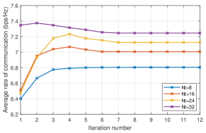
(b) The average rate of communication versus the number of iterations for $N_{t}=8,16,24,32$.

Figure 2: Convergence of the proposed algorithm.

This subsection aims at analyzing the convergence performance of the proposed algorithm considering different numbers of antennas. We assume that the number of receive antennas $N_{r}$ is set equal to $N_{t}$. The numbers of communication users and sensing targets are $C=2$ and $K=2$, respectively.

Fig. 2LABEL:sub@convergence_MI shows the sensing MI versus iteration number. It can be observed that the sensing MI increases along with the iteration monotonously for all considered conditions. It is noted that the average number of iterations that makes the sensing MI converge is about 5. The average rate of communication versus iteration number is also depicted in Fig. 2LABEL:sub@convergence_SINR. Besides, it can be observed in Fig. 2LABEL:sub@convergence_MI and Fig. 2LABEL:sub@convergence_SINR that the number of iterations required in the algorithm increases with the increase of $N_{t}$, because the increase of antenna numbers enlarges the feasible set $\left\{{\mathbf{R}}_{1},\ldots,{\mathbf{R}}_{C+M}\right\}$.

V-B Beampattern Performance

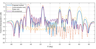
(a) The optimized transmit beampatterns with $K=3$.

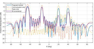
(b) The optimized transmit beampatterns with $K=2$.

Figure 3: The transmit beampattern for the proposed method and benchmarks.

In this subsection, we show the optimized beampattern performance for different $K$ values. We assume $C=2$ users at the location $\theta_{C1}=-45^{\circ}$ and $\theta_{C2}=-15^{\circ}$, respectively. The SINR constraint of each communication user is ${{\Gamma}_{i}}=5{\rm\ dB},\forall i\in\mathcal{C}$. And the threshold of sensing MI is $\Lambda=10{\rm\ bits}$. The beampatterns obtained via the mentioned schemes are depicted in Fig. 3LABEL:sub@beampattern_k3 for $K=3$ targets located at $20^{\circ}$, $40^{\circ}$, $60^{\circ}$ and in Fig. 3LABEL:sub@beampattern_k2 for $K=2$ targets located at $20^{\circ}$, $40^{\circ}$.

It can be seen from Fig. 3LABEL:sub@beampattern_k3 that the proposed method has three radar mainlobes, matching the locations of the Radar-only design. However, there are only two radar mainlobes located at around $20^{\circ}$ and $40^{\circ}$ for the MI-constrained approach. We note that the DoF for MIMO beamforming is determined by the rank of the covariance matrix[13]. In the MI-constrained approach, only $C=2$ communication streams are transmitted, and thus the DoF is no larger than the number of users $C$. If $C$ is less than the rank of the optimal Radar-only design covariance matrix, the MI-constrained approach cannot provide enough DoF to synthesize the desired radar beams, explaining the degraded beampattern observed in Fig. 3LABEL:sub@beampattern_k3. The proposed method simultaneously transmits $C$ transmission streams and $M$ probing streams, which can provide enough DoF for transmit beamforming, and thus can produce the beampatterns close to that of the optimal Radar-only method. In Fig. 3LABEL:sub@beampattern_k2, however, it is clearly observed that the proposed approach has enough DoF to generate a beampattern similar to that of the Radar-only method for $K=2$ targets.

V-C Comparisons of Communication and Sensing Performance

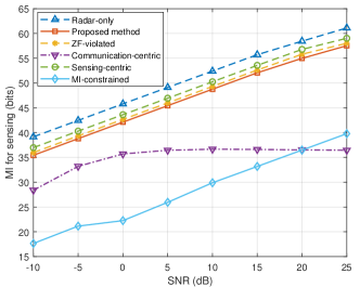
Figure 4: The sensing MI versus receive SNR.

In Fig. 4, we show the sensing MI versus the received SNR of the echo signal for the various beamforming schemes. The numbers of communication users and sensing targets are $C=2$ and $K=2$, respectively. We observe that the Radar-only approach achieves the highest sensing MI among the compared schemes since it is not constrained by communication performance. Subsequently, the Sensing-centric scheme achieves sensing MI second only to Radar-only case, as it focuses solely on meeting the minimum communication performance requirements, with the remaining transmit power allocated towards enhancing sensing capabilities. The proposed method exhibits superior sensing MI performance over the MI-constrained and Communication-centric schemes. It is also noted that the sensing MI of the Communication-centric scheme increases very slowly with SNR, as this scheme solely focuses on meeting the minimum sensing MI requirement, allocating the remaining transmit power to improve the communication SINR for each user. Additionally, we observe that the proposed method closely approaches the ZF-violated scheme. This indicates that the impact of cross-correlation constraints (27c) on the achievable maximum sensing MI is minimal. Nevertheless, in order to fully compare ZF-violated scheme with the proposed method to demonstrate the impact of cross-correlation constraints on overall performance, it is also necessary to consider communication performance.

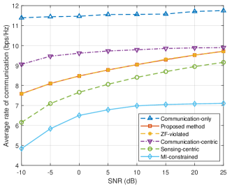
Figure 5: The average rate of the MU-MIMO communication versus SNR.

Fig. 5 unfolds the average achievable communication rate versus communication SNR under the same settings as in Fig. 4. It is observed that the Communication-only scheme achieves the best average communication rate, while other schemes experience communication performance loss due to sensing MI constraints. The propose method demonstrates superior average communication rate compared to the MI-constrained scheme. This is due to the fact that the MI-constrained approach optimizes the lower bound of SINR, which cannot attain the same communication performance as the proposed method that directly optimizes SINRs. Moreover, the performance gap between the proposed method and the Communication-centric approach diminishes as SNR increases, converging closely at high SNR levels. We observe that the average communication rate of the proposed method closely approximates that of the ZF-violated scheme, suggesting that cross-correlation constraints do not compromise the communication performance either.

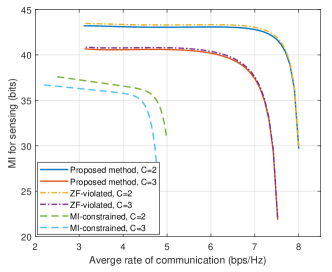
Figure 6: The tradeoff between the sensing MI and the average rate of the MU-MIMO communication.

In Fig. 6, we evaluate the tradeoff between the average communication rate and the sensing MI for $C=2$ and $C=3$. For the proposed method, the weight of sensing MI $\alpha$ varies from $0.1$ to $0.9$. The weights of different communication users are set with the same value, calculated by ${\omega}_{i}=(1-\alpha)/C,\forall i\in\mathcal{C}$. The weights of different sensing targets are equivalently established as ${\xi}_{k}=\alpha/K,\forall k$. The threshold $\rho$ utilized in the MI-constrained approach varies from $0.2$ to $0.9$. In the case where the number of users and targets are the same, the proposed method achieves higher sensing MI than the MI-constrained scheme with the same communication average rate. Similarly, when to achieve the same sensing MI, the proposed method obtains a better average communication rate. This indicates that the proposed method provides a better trade-off between multi-target sensing performance and multi-user communication performance compared to the MI-constrained scheme. It is also noted that the proposed method and the ZF-violated scheme exhibit a similar trade-off, demonstrating that the cross-correlation constraints does not compromise the overall performance of the ISAC system. Furthermore, we observe that the more users the ISAC system has to communicate with reliably, the lower the sensing MI is achieved in the proposed method. This is because ensuring an additional communication user performance requires utilizing transmit power resources originally allocated for sensing.

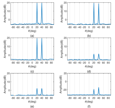
Figure 7: Capon spatial spectrum, for $K=2$. (a) Capon spatial spectrum for the Radar-only approach without radar signals. (b) Capon spatial spectrum for the proposed method. (c) Capon spatial spectrum for the proposed method without radar signals. (d) Capon spatial spectrum for the ZF-violated scheme. (e) Capon spatial spectrum for the ZF-violated scheme without radar signals. (f) Capon spatial spectrum for the MI-contrained scheme.

Since the sensing MI is not the only performance measure for sensing, we also examine the angle estimation performance obtained by using the Capon method. We simulate two radar targets located at directions $20^{\circ}$ and $40^{\circ}$, respectively. The complex amplitude of the targets are both $1$[13]. Fig. 7 exhibits the Capon spatial spectrum with and without transmitting radar signals for several benchmarks in one test. Without transmitting radar signals, it can be observed from Fig 7 (a), (c), (e), and (f) that the proposed method exhibits an angular resolution close to that of the Radar-only approach and yields significantly higher peak values at the desired target directions compared to other ZF-violated and MI-constrained schemes. We also observe that when the number of targets does not exceed the number of users, all schemes can effectively detect and estimate the targets regardless of whether additional radar signals are transmitted.

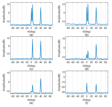
Figure 8: Capon spatial spectrum, for $K=3$. (a) Capon spatial spectrum for the Radar-only approach. (b) Capon spatial spectrum for the proposed method. (c) Capon spatial spectrum for the proposed method without radar signals. (d) Capon spatial spectrum for the ZF-violated scheme. (e) Capon spatial spectrum for the ZF-violated scheme without radar signals. (f) Capon spatial spectrum for the MI-contrained scheme.

Then, we consider the scenario where there are three targets, with two of them placed closely. The directions of the targets are $0^{\circ}$, $5^{\circ}$ and $40^{\circ}$, and the complex amplitude for each target is $1$[13]. When transmitting radar signals, it can be observed that the peak at the location of $0^{\circ}$ in Fig 8 (d) is not prominent compared with Fig 8 (b), resulting in an inadequate resolution of two closely spaced targets. This observation highlights that the proposed method enhances the ability to resolve multiple targets by suppressing the cross-correlation among signals reflected from different targets through constraints (27c). Additionally, it can be observed from Fig 8 (c), (e) and (f) that when the BS transmits only communication signals, all three targets cannot be effectively distinguished, with only two of them exhibiting significant peaks. This is due to the fact that when only communication signals are transmitted, the rank of the transmitted signal covariance matrix is limited by $C$, which cannot provide sufficient DoFs to form three beams to cover all three targets.

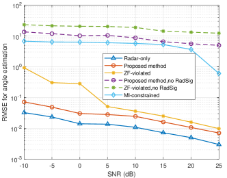
Figure 9: RMSE for angle estimation versus receive SNR, for $K=3$.

Fig 9 shows the root-mean-square-error (RMSE) of target angle estimation versus radar SNR. The angles of targets are estimated by finding the peaks in the Capon spatial spectrum. When radar signals are not transmitted, the RMSE for the proposed scheme, the ZF-violated scheme, and the MI-constrained scheme is significantly higher compared to other schemes that utilize radar signals. This is due to the insufficient DoFs, often resulting in the inability to detect targets close to the true target direction, which aligns with the conclusion in Fig 8. Additionally, we observe that when radar signals are transmitted, the proposed scheme exhibits a lower RMSE compared to the ZF-violated scheme and is close to the Radar-only scheme. This indicates that even with similar capabilities in maximizing sensing MI, the proposed scheme outperforms ZF-violated in terms of angular estimation performance. Therefore, the sensing MI upper bound with cross-correlation constraints is more appropriate performance metric for multi-target sensing.

VI Conclusion

In this paper, we investigated a multi-objective optimization framework for ISAC beamforming that provides a flexible tradeoff between multiple targets sensing and multi-user communication. We formulate a MOOP based on the tight upper bound of sensing MI and each user’s SINR. Then, we employ a max-min utility function method to obtain specific Pareto optimal solutions while considering fairness between users and sensing targets. Numerical results were presented for validating the proposed beamforming method and provided the useful insights. Firstly, the proposed method can achieve superior performance boundaries of communication and sensing performance, while also facilitating a flexible tradeoff between them. Secondly, the proposed method can enhance target resolution and angle estimation accuracy for multiple targets, thereby validating the suitability of constrained sensing MI upper bound as a performance metric for multi-target sensing.

Extending the proposed framework to practical scenarios with imperfect channel state information (CSI) may degrade the communication and sensing performance, necessitating the development of robust beamforming techniques that account for channel uncertainties. Additionally, dynamic target tracking in non-ideal conditions can be computationally demanding, requiring the development of low-complexity tracking algorithms and efficient beamforming update schemes. Future research should focus on investigating the robustness of the MI-based beamforming method under imperfect CSI and developing advanced techniques to mitigate its impact while enabling real-time adaptation for practical implementation.

Appendix A Proof of Theorem 1

Substituting (10) into (III), the sensing MI can be simplified to (42), presented at the top of the next page.

$$I\left({{{\mathbf{\tilde{y}}}}_{r}};\mathbf{\tilde{g}}\left|{\mathbf{\tilde{X}}}\right.\right) =\log\left[\det\left(\mathbf{I}+\frac{1}{\sigma_{r}^{2}}\left(\sum\limits_{t=1}^{K}{\sigma_{k}^{2}\left({{\mathbf{X}}^{*}}{{\mathbf{X}}^{T}}\otimes{{\mathbf{I}}_{{{N}_{r}}}}\right)\text{vec}\left(\mathbf{A}\left({{\theta}_{k}}\right)\right)}\text{vec}{{\left(\mathbf{A}\left({{\theta}_{k}}\right)\right)}^{H}}\right)\right)\right]$$ (42a)

$$=\log\left[\det\left(\mathbf{I}+\frac{1}{\sigma_{r}^{2}}\left(\sum\limits_{t=1}^{K}{\sigma_{k}^{2}\text{vec}\left(\mathbf{A}\left({{\theta}_{k}}\right)\left(\mathbf{X}{{\mathbf{X}}^{H}}\right)\right)}\text{vec}{{\left(\mathbf{A}\left({{\theta}_{k}}\right)\right)}^{H}}\right)\right)\right],$$ (42b)

 

The derivation of (42b) follows the fact that $\text{vec}(\mathbf{ABC})=({{\mathbf{C}}^{T}}\otimes\mathbf{A})\text{vec}(\mathbf{B})$.

Then, by introducing auxiliary block matrices

$$\mathbf{T}=\frac{1}{\sigma_{r}^{2}}\left[\text{vec}\left(\!\mathbf{A}\left({{\theta}_{1}}\right)\!\left(\mathbf{X}{{\mathbf{X}}^{H}}\right)\!\right)\!,\ldots,\text{vec}\left(\mathbf{A}\left({{\theta}_{K}}\!\right)\!\left(\mathbf{X}{{\mathbf{X}}^{H}}\right)\right)\right],$$ (43)

$$\mathbf{M}={{\left[\sigma_{1}^{2}\text{vec}\left(\mathbf{A}\left({{\theta}_{1}}\right)\right),\ldots,\sigma_{K}^{2}\text{vec}\left(\mathbf{A}\left({{\theta}_{K}}\right)\right)\right]}^{H}},$$

the sensing MI in (42b) can be rewritten as

$$I\left({{{\mathbf{\tilde{y}}}}_{r}};\mathbf{\tilde{g}}\left|{\mathbf{\tilde{X}}}\right.\right) =\log\left[\det\left(\mathbf{I}+\mathbf{TM}\right)\right]=\log\left[\det\left(\mathbf{I}+\mathbf{MT}\right)\right],$$ (44)

where the last equality follows from Sylvester’s determinant identity $\det(\mathbf{I}+\mathbf{AB})=\det(\mathbf{I}+\mathbf{BA})$. The $(i,j)$-th entry of $\mathbf{MT}$ is given by

$${{\left[\mathbf{MT}\right]}_{i,j}} =\frac{\sigma_{i}^{2}}{\sigma_{r}^{2}}\text{ve}{{\text{c}}^{H}}\left(\mathbf{A}\left({{\theta}_{i}}\right)\right)\text{vec}\left(\mathbf{A}\left({{\theta}_{j}}\right)\left(\mathbf{X}{{\mathbf{X}}^{H}}\right)\right)$$ (45)

$$=\frac{L\sigma_{i}^{2}}{\sigma_{r}^{2}}\text{tr}\left({{\mathbf{A}}^{H}}\left({{\theta}_{i}}\right)\mathbf{A}\left({{\theta}_{j}}\right){{\mathbf{R}}_{X}}\right)=\sigma_{i}^{2}{{\left[\mathbf{\Phi}\right]}_{i,j}},$$

where the derivation of (45) utilizes the identity $\text{ve}{{\text{c}}^{H}}\left(\mathbf{A}\right)\text{vec}\left(\mathbf{B}\right)=\text{tr}\left({{\mathbf{A}}^{H}}\mathbf{B}\right)$, and ${{\left[\mathbf{\Phi}\right]}_{i,j}}$ denotes the $(i,j)$-th element of the matrix $\mathbf{\Phi}\in\mathbb{C}^{K\times K}$. Next, we define a diagonal matrix $\mathbf{\Lambda}\in\mathbb{C}^{K\times K}$ as

$$\mathbf{\Lambda}\triangleq\text{diag}\left\{\frac{1}{\sigma_{1}^{2}},\frac{1}{\sigma_{2}^{2}},\ldots,\frac{1}{\sigma_{K}^{2}}\right\}.$$ (46)

By extracting the constant coefficient terms $\{\sigma_{1}^{2},\ldots,\sigma_{K}^{2}\}$ from determinant by row, the sensing MI is recast as

$$I\left({{{\mathbf{\tilde{y}}}}_{r}};\mathbf{\tilde{g}}\left|{\mathbf{\tilde{X}}}\right.\right) =\log\left[\det\left(\mathbf{\Phi}+\mathbf{\Lambda}\right)\prod\limits_{k=1}^{K}\sigma_{k}^{2}\right],$$ (47)

which completes the proof of Lemma 1.

Appendix B Proof of Lemma 2

We first prove that $\mathcal{M}$ is a compact set. Following [42], we know that the feasible transmit strategy set $\mathcal{R}$ is compact. According to [46], the continuous mapping of a compact set is also a compact set. Since the upper bound of sensing MI $I_{\rm up}$ and each user’s SINR ${\gamma}_{i}$ are all continuous functions of $\left\{{{\mathbf{R}}_{1}},\ldots,{{\mathbf{R}}_{{{C}}+M}}\right\}\in{\mathcal{R}}$, $\mathcal{M}$ is a compact set.

To prove that $\mathcal{M}$ is a normal set, we use a similar method as described in [14, Appx.A]. Take $\mathbf{x}=\left({{I}_{\rm up}},{{\gamma}_{1}},\cdots,{{\gamma}_{{{C}}}}\right)\in\mathcal{M}$ and assume that $\left({{\mathbf{R}}_{1}},\ldots,{{\mathbf{R}}_{{{C}}+M}}\right)$ is a feasible strategy that attains point $\mathbf{x}$. Our goal is to prove that any given $\mathbf{x}^{\prime}=\left({I^{\prime}}_{\rm up},{\gamma^{\prime}}_{1},\cdots,{\gamma^{\prime}}_{C}\right)$ satisfying $\mathbf{x}^{\prime}\leq\mathbf{x}$ also belongs to $\mathcal{M}$.

To this end, we represent the transmit beamforming strategy in a new form $\left({{p}_{1}}{{\mathbf{R}}_{1}},\ldots,{{p}_{{{C}}+M}}{{\mathbf{R}}_{{{C}}+M}}\right)$, where $\left({{p}_{1}},\ldots,{{p}_{{{C}}+M}}\right)\in\mathcal{P}$ is a set of power allocation coefficients that should belong to

$$\mathcal{P}=\{ \left({{p}_{1}},\ldots,{{p}_{{{C}}+M}}\right):p_{n}>0,\text{tr}\left(\sum\nolimits_{n=1}^{{{C}}+M}{{{p}_{n}}{{\mathbf{R}}_{n}}}\right)\leq{{P}_{T}},$$ (48)

$$\text{tr}\left(\mathbf{a}\left({{\theta}_{i}}\right){{\mathbf{a}}^{H}}\left({{\theta}_{j}}\right)\left(\sum\nolimits_{n=1}^{{{C}}+M}{{{p}_{n}}{{\mathbf{R}}_{n}}}\right)\right)=0\quad(i\neq j)\}.$$

First, we need to find that $\left({{p}_{1}},\ldots,{{p}_{{{C}}+M}}\right)\in\mathcal{P}$ satisfies the given SINRs and $I_{\rm up}$, i.e.,

$${{\gamma}_{i}}=\frac{{{p}_{i}}\mathbf{h}_{i}^{H}{{\mathbf{R}}_{i}}{{\mathbf{h}}_{i}}}{\sum\nolimits_{j=1,j\neq i}^{{{C}}+M}{{{p}_{j}}\mathbf{h}_{i}^{H}{{\mathbf{R}}_{j}}{{\mathbf{h}}_{i}}}+\sigma_{c}^{2}},\forall i\in\mathcal{C},$$ (49a)

$${{I}_{\rm up}}=\sum\limits_{{k}=1}^{K}{\log\!\left(\!\!1+\!\frac{{{N}_{r}}\sigma_{k}^{2}L}{\sigma_{r}^{2}}{{\mathbf{a}}^{H}}\!\!\left({{\theta}_{k}}\right)\!\left(\!\sum\limits_{n=1}^{C+M}{p_{n}}{{\mathbf{R}}_{n}}\right)\!\mathbf{a}\left({{\theta}_{k}}\right)\!\!\right)}.$$ (49b)

For (49a), given arbitrary $\left({{p}_{C+1}},\ldots,{{p}_{{{C}}+M}}\right)$ satisfying each element $p_{i}\in(0,1]$, we can derive the following equation, i.e.,

$$\mathbf{\Gamma}\left({\mathbf{A}_{1}}{\mathbf{p}_{1}}+{\mathbf{A}_{2}}{\mathbf{p}_{2}}+\mathbf{b}\right)=\mathbf{p}_{1},$$ (50)

where $\mathbf{\Gamma}=\text{diag}\left({{\gamma}_{i}},\ldots,{{\gamma}_{{{C}}}}\right)$, $\mathbf{p}_{1}=\!{{\left[{{p}_{1}},\ldots,{{p}_{{{C}}}}\right]}^{T}}$, $\mathbf{p}_{2}=\!{{\left[{{p}_{C+1}},\ldots,{{p}_{C+M}}\right]}^{T}}$,

$$\mathbf{A}_{1}=\left[\begin{matrix}0&a_{1,2}&\cdots&a_{1,C}\\ a_{2,1}&0&\cdots&a_{2,C}\\ \vdots&\vdots&\ddots&\vdots\\ a_{C,1}&a_{C,2}&\cdots&0\end{matrix}\right],$$ (51)

$$\mathbf{A}_{2}=\left[\begin{matrix}a_{1,C+1}&\cdots&a_{1,C+M}\\ a_{2,C+1}&\cdots&a_{2,C+M}\\ \vdots&\ddots&\vdots\\ a_{C,C+1}&\cdots&a_{C,C+M}\end{matrix}\right],$$ (52)

with

$${{a}_{i,j}}=\frac{\mathbf{h}_{i}^{H}{{\mathbf{R}}_{j}}{{\mathbf{h}}_{i}}}{\mathbf{h}_{i}^{H}{{\mathbf{R}}_{i}}{{\mathbf{h}}_{i}}},$$ (53)

and $\mathbf{b}={{\left[{{b}_{1}},\ldots,{{b}_{{{C}}}}\right]}^{T}}\in{{\mathbb{R}}^{{{C}}\times 1}}$ with

$${{b}_{i}}=\frac{\sigma_{c}^{2}}{\mathbf{h}_{i}^{H}{{\mathbf{R}}_{i}}{{\mathbf{h}}_{i}}}.$$ (54)

Based on (50), we can obtain that

$$\mathbf{p}_{1} ={{\left(\mathbf{I}-{\mathbf{\Gamma}}{{\mathbf{A}}_{1}}\right)}^{-1}}{\left({\mathbf{\Gamma}}{\mathbf{A}_{2}}{\mathbf{p}_{2}}+{\mathbf{\Gamma}}\mathbf{b}\right)}$$ (55)

$$\overset{\left(a\right)}{=}\left(\mathbf{I}+\sum\limits_{n=1}^{\infty}{{{\left({\mathbf{\Gamma}}{{\mathbf{A}}_{1}}\right)}^{n}}}\right){\left({\mathbf{\Gamma}}{\mathbf{A}_{2}}{\mathbf{p}_{2}}+{\mathbf{\Gamma}}\mathbf{b}\right)},$$

where $(a)$ is based on the Neumann series approximation[47] of ${{\left(\mathbf{I}-{\mathbf{\Gamma}}{{\mathbf{A}}_{1}}\right)}^{-1}}$. Since all elements in ${{\mathbf{A}}_{1}}$, ${{\mathbf{A}}_{2}}$, $\mathbf{p}_{2}$ and $\mathbf{b}$ are non-negative, it indicates that each element in $\mathbf{p}_{1}$ is obtained from a polynomial with positive coefficients in ${{\gamma}_{i}},\ldots,{{\gamma}_{{{C}}}}$. Therefore, a decrease in $\gamma_{i}$ will necessarily lead to a decrease in at least one of the power allocation coefficients $\left({{p}_{1}},\ldots,{{p}_{{{C}}}}\right)$. For (49b), $I_{\rm up}$ can be further rewritten as

$${{I}_{\rm up}}=\log\left(\prod\nolimits_{k=1}^{K}{\left(1+\sum\nolimits_{n=1}^{C+M}{{{p}_{n}}{{d}_{nk}}}\right)}\right),$$ (56)

where ${d}_{nk}$ is a positive constant given as

$${d}_{nk}=\frac{{{N}_{r}}\sigma_{k}^{2}L}{\sigma_{r}^{2}}{{\mathbf{a}}^{H}}\left({{\theta}_{k}}\right){\mathbf{R}}_{n}\mathbf{a}\left({{\theta}_{k}}\right),\forall n,k.$$ (57)

From (56), it is evident that $I_{\rm up}$ can be expressed as the logarithm of a polynomial in ${{p}_{1}},\ldots,{p}_{C+M}$ with positive coefficients. As the logarithm function is monotonically increasing, a reduction in $I_{\rm up}$ will inevitably result in a decrease in at least one of the power allocation coefficients $\left({{p}_{1}},\ldots,{{p}_{C+M}}\right)$.

In summary, based on the above analysis, we can conclude that for any ${\gamma^{\prime}}_{i}\leq{{\gamma}_{i}},\forall i$ or ${I^{\prime}}_{\rm up}\leq{{I}_{\rm up}}$, we can always properly find $\mathbf{p}^{\prime}\in\mathcal{P}$ satisfying that $\mathbf{p}^{\prime}\leq\mathbf{p}$, and making $\left({{p}^{\prime}_{1}}{{\mathbf{R}}_{1}},\ldots,{{p}^{\prime}_{{{C}}+M}}{{\mathbf{R}}_{{{C}}+M}}\right)$ a feasible solution that attains point $\mathbf{x}^{\prime}$. This implies that if $\mathbf{x}^{\prime}\in\mathbb{R}_{+}^{n}$ and satisfies $\mathbf{x}^{\prime}\leq\mathbf{x}$, then $\mathbf{x}^{\prime}$ belongs to $\mathcal{M}$. In other words, the achievable performance region $\mathcal{M}$ is a normal set, which completes the proof.

Appendix C Proof of Theorem 2

The optimal values of (36) is denoted as $\left(I_{\rm up}^{*},\gamma_{1}^{*},\cdots,\gamma_{C}^{*}\right)$, and the corresponding optimal solution with arbitrary ranks as

$$\left\{\mathbf{R}_{1}^{*},\ldots,\mathbf{R}_{{C}+M}^{*}\right\}.$$ (58)

We need to prove that the rank-one optimal solution $\left\{{{{\mathbf{\bar{R}}}}_{1}},\ldots,{{{\mathbf{\bar{R}}}}_{{C}+M}}\right\}$ can be constructed from (58). First, we construct $\left\{{{{\mathbf{\bar{R}}}}_{1}},\ldots,{{{\mathbf{\bar{R}}}}_{C}}\right\}$ as

$${{\mathbf{\bar{R}}}_{i}}={{\mathbf{\bar{w}}}_{i}}\mathbf{\bar{w}}_{i}^{H},\forall i\in\mathcal{C},$$ (59)

where

$${{\mathbf{\bar{w}}}_{i}}=\frac{\mathbf{R}_{i}^{*}{{\mathbf{h}}_{i}}}{\sqrt{\mathbf{h}_{i}^{H}\mathbf{R}_{i}^{*}{{\mathbf{h}}_{i}}}},\forall i\in\mathcal{C},$$ (60)

It can be readily verified that

$$\mathbf{h}_{i}^{H}{{\mathbf{\bar{R}}}_{i}}{{\mathbf{h}}_{i}}=\mathbf{h}_{i}^{H}{{\mathbf{\bar{w}}}_{i}}\mathbf{\bar{w}}_{i}^{H}\mathbf{h}=\mathbf{h}_{i}^{H}\mathbf{R}_{i}^{*}{{\mathbf{h}}_{i}},\forall i\in\mathcal{C},$$ (61)

By noting the above fact, we next construct $\left\{{{{\mathbf{\bar{R}}}}_{C+1}},\ldots,{{{\mathbf{\bar{R}}}}_{C+M}}\right\}$. Let ${{\mathbf{R}}_{r}}\triangleq\sum\nolimits_{n=1}^{{C}+M}{\mathbf{R}_{n}^{*}}-\sum\nolimits_{n=1}^{{C}}{{{{\mathbf{\bar{R}}}}_{n}}}=\sum\nolimits_{n=C+1}^{C+M}{{{{\mathbf{\bar{R}}}}_{n}}}$. Therefore, we need to prove that ${{\mathbf{R}}_{r}}$ is semidefinite. Since $\sum\nolimits_{n=C+1}^{{C}+M}{\mathbf{R}_{n}^{*}}$ is semidefinite due to (27d), we only need to prove that $\mathbf{R}_{i}^{*}-{{\mathbf{\bar{R}}}_{i}}\succeq 0$ for all $i\leqslant C$.

For any $\mathbf{x}\in{{\mathbb{C}}^{N_{t}}}$, it holds that

$${{\mathbf{x}}^{H}}\left(\mathbf{R}_{i}^{*}-{{{\mathbf{\bar{R}}}}_{i}}\right)\mathbf{x}={{\mathbf{x}}^{H}}\mathbf{R}_{i}^{*}\mathbf{x}-\frac{{{\left|{{\mathbf{x}}^{H}}\mathbf{R}_{i}^{*}{{\mathbf{h}}_{i}}\right|}^{2}}}{\left(\mathbf{h}_{i}^{H}\mathbf{R}_{i}^{*}{{\mathbf{h}}_{i}}\right)}.$$ (62)

According to Cauchy-Schwarz inequality, we have

$$\left(\mathbf{h}_{i}^{H}\mathbf{R}_{i}^{*}{{\mathbf{h}}_{i}}\right)\left({{\mathbf{x}}^{H}}\mathbf{R}_{i}^{*}\mathbf{x}\right)\geq{{\left|{{\mathbf{x}}^{H}}\mathbf{R}_{i}^{*}{{\mathbf{h}}_{i}}\right|}^{2}},$$ (63)

which means that

$${{\mathbf{x}}^{H}}\left(\mathbf{R}_{i}^{*}-{{{\mathbf{\bar{R}}}}_{i}}\right)\mathbf{x}\geq 0,\ \forall\mathbf{x}\in{{\mathbb{C}}^{N}},$$ (64)

i.e., ${{\mathbf{R}}_{r}}\succeq 0$.

By taking the Cholesky decomposition of ${{\mathbf{R}}_{r}}$, we have

$${{\mathbf{\bar{W}}}_{r}}\mathbf{\bar{W}}_{r}^{H}=\sum\nolimits_{n=1}^{C+M}{\mathbf{R}_{n}^{*}}-\sum\nolimits_{n=1}^{C}{{{{\mathbf{\bar{R}}}}_{n}}},$$ (65)

where ${{\mathbf{\bar{W}}}_{r}}=\left[{{{\mathbf{\bar{w}}}}_{{C}+1}},\ldots,{{{\mathbf{\bar{w}}}}_{{C}+M}}\right]$ is a lower triangular matrix. So we obtain that ${{\mathbf{\bar{R}}}_{j}}={{\mathbf{\bar{w}}}_{j}}\mathbf{\bar{w}}_{j}^{H}$ for $j=C+1,\ldots,C+M$. It follows that

$$\sum\nolimits_{n=1}^{{C}+M}{\mathbf{R}_{n}^{*}}=\sum\nolimits_{n=1}^{{C}+M}{{{{\mathbf{\bar{R}}}}_{n}}}.$$ (66)

Now we need to validate that $\left\{{{{\mathbf{\bar{R}}}}_{1}},\ldots,{{{\mathbf{\bar{R}}}}_{{C}+M}}\right\}$ is a feasible solution to (36). And we have

$$\text{tr}\left(\sum\nolimits_{n=1}^{C+M}{{{{\mathbf{\bar{R}}}}_{n}}}\right)=\text{ tr}\left(\sum\nolimits_{n=1}^{C+M}{\mathbf{R}_{n}^{*}}\right)\leq{{P}_{T}},$$ (67)

$$\text{tr}\left(\mathbf{a}\left({{\theta}_{i}}\right){{\mathbf{a}}^{H}}\left({{\theta}_{j}}\right)\left(\sum\nolimits_{n=1}^{{C}+M}{{{{\mathbf{\bar{R}}}}_{n}}}\right)\right)=$$

$$\text{tr}\left(\mathbf{a}\left({{\theta}_{i}}\right){{\mathbf{a}}^{H}}\left({{\theta}_{j}}\right)\left(\sum\nolimits_{n=1}^{{C}+M}{\mathbf{R}_{n}^{*}}\right)\right)\!=\!0\left(i\neq j\right),$$

which means that the constraints of (36) hold for $\{{{{\mathbf{\bar{R}}}}_{1}},\ldots,{{{\mathbf{\bar{R}}}}_{{C}+M}}\}$.

Based on (61), we have

$${I_{\rm up}^{*}} =\sum\nolimits_{{k}=1}^{K}{\log\!\left(1+\!\frac{{{N}_{r}}\sigma_{k}^{2}L}{\sigma_{r}^{2}}{{\mathbf{a}}^{H}}\!\!\left({{\theta}_{k}}\right)\!\left(\!\sum\limits_{n=1}^{C+M}{\mathbf{R}_{n}^{*}}\right)\!\mathbf{a}\left({{\theta}_{k}}\right)\right)}$$ (68)

$$=\sum\nolimits_{{k}=1}^{K}{\log\!\left(1+\!\frac{{{N}_{r}}\sigma_{k}^{2}L}{\sigma_{r}^{2}}{{\mathbf{a}}^{H}}\!\!\left({{\theta}_{k}}\right)\!\left(\!\sum\limits_{n=1}^{C+M}{{{{\mathbf{\bar{R}}}}_{n}}}\right)\!\mathbf{a}\left({{\theta}_{k}}\right)\right)},$$

$${\gamma_{i}^{*}} =\frac{\mathbf{h}_{i}^{H}\mathbf{R}_{i}^{*}{{\mathbf{h}}_{i}}}{\mathbf{h}_{i}^{H}\left(\sum\nolimits_{n=1}^{{C}+M}{\mathbf{R}_{n}^{*}}\right){{\mathbf{h}}_{i}}-\mathbf{h}_{i}^{H}\mathbf{R}_{i}^{*}{{\mathbf{h}}_{i}}+\sigma_{c}^{2}}$$ (69)

$$=\frac{\mathbf{h}_{i}^{H}{{{\mathbf{\bar{R}}}}_{i}}{{\mathbf{h}}_{i}}}{\mathbf{h}_{i}^{H}\left(\sum\nolimits_{n=1}^{{C}+M}{{{{\mathbf{\bar{R}}}}_{n}}}\right){{\mathbf{h}}_{i}}-\mathbf{h}_{i}^{H}{{{\mathbf{\bar{R}}}}_{i}}{{\mathbf{h}}_{i}}+\sigma_{c}^{2}},$$

which means that the optimal values do not change.

Above all, $\{{{{\mathbf{\bar{R}}}}_{1}},\ldots,{{{\mathbf{\bar{R}}}}_{{C}+M}}\}$ is also the optimal solution to (36), which completes the proof.

References

- [1] F. Liu, C. Masouros, A. P. Petropulu, H. Griffiths, and L. Hanzo, “Joint radar and communication design: Applications, state-of-the-art, and the road ahead,” IEEE Trans. Commun., vol. 68, no. 6, pp. 3834–3862, Feb. 2020.
- [2] F. Liu, Y. Cui, C. Masouros, J. Xu, T. X. Han, Y. C. Eldar, and S. Buzzi, “Integrated sensing and communications: Toward dual-functional wireless networks for 6G and beyond,” IEEE J. Select. Areas Commun., vol. 40, no. 6, pp. 1728–1767, Mar. 2022.
- [3] D. Ma, N. Shlezinger, T. Huang, Y. Liu, and Y. C. Eldar, “Joint radar-communication strategies for autonomous vehicles: Combining two key automotive technologies,” IEEE Signal Processing Mag., vol. 37, no. 4, pp. 85–97, Jun. 2020.
- [4] Z. Feng, Z. Wei, X. Chen, H. Yang, Q. Zhang, and P. Zhang, “Joint communication, sensing, and computation enabled 6G intelligent machine system,” IEEE Network, vol. 35, no. 6, pp. 34–42, Nov. 2021.
- [5] X. Li, M. Zhang, H. Chen, C. Han, L. Li, D.-T. Do, S. Mumtaz, and A. Nallanathan, “UAV-enabled multi-pair massive MIMO-NOMA relay systems with low-resolution ADCs/DACs,” IEEE Trans. Veh. Technol., vol. 73, no. 2, pp. 2171–2186, Feb. 2024.
- [6] Y. Cheng, J. Du, J. Liu, L. Jin, X. Li, and D. B. da Costa, “Nested tensor-based framework for ISAC assisted by reconfigurable intelligent surface,” IEEE Trans. Veh. Technol., vol. 73, no. 3, pp. 4412–4417, Mar. 2024.
- [7] J. A. Zhang, F. Liu, C. Masouros, R. W. Heath, Z. Feng, L. Zheng, and A. Petropulu, “An overview of signal processing techniques for joint communication and radar sensing,” IEEE J. Sel. Top. Sign. Proces., vol. 15, no. 6, pp. 1295–1315, Sept. 2021.
- [8] J. A. Zhang, M. L. Rahman, K. Wu, X. Huang, Y. J. Guo, S. Chen, and J. Yuan, “Enabling joint communication and radar sensing in mobile networks—a survey,” IEEE Commun. Surv. Tutor., vol. 24, no. 1, pp. 306–345, Oct. 2022.
- [9] X. Fang, W. Feng, Y. Chen, N. Ge, and Y. Zhang, “Joint communication and sensing toward 6G: Models and potential of using MIMO,” IEEE Internet of Things Journal, vol. 10, no. 5, pp. 4093–4116, 2023.
- [10] Z. Wang, X. Mu, and Y. Liu, “Near-field integrated sensing and communications,” IEEE Commun. Lett., vol. 27, no. 8, pp. 2048–2052, Aug. 2023.
- [11] F. Liu, C. Masouros, A. Li, H. Sun, and L. Hanzo, “MU-MIMO communications with MIMO radar: From co-existence to joint transmission,” IEEE Transactions on Wireless Communications, vol. 17, no. 4, pp. 2755–2770, 2018.
- [12] X. Liu, T. Huang, and Y. Liu, “Transmit design for joint MIMO radar and multiuser communications with transmit covariance constraint,” IEEE J. Sel. Areas Commun., vol. 40, no. 6, pp. 1932–1950, Mar. 2022.
- [13] X. Liu, T. Huang, N. Shlezinger, Y. Liu, J. Zhou, and Y. C. Eldar, “Joint transmit beamforming for multiuser MIMO communications and MIMO radar,” IEEE Trans. Signal Process., vol. 68, pp. 3929–3944, Jun. 2020.
- [14] L. Chen, F. Liu, W. Wang, and C. Masouros, “Joint radar-communication transmission: A generalized pareto optimization framework,” IEEE Trans. Signal Process., vol. 69, pp. 2752–2765, 2021.
- [15] Z. Ni, J. A. Zhang, K. Yang, X. Huang, and T. A. Tsiftsis, “Multi-metric waveform optimization for multiple-input single-output joint communication and radar sensing,” IEEE Trans. Commun., vol. 70, no. 2, pp. 1276–1289, Dec. 2022.
- [16] X. Yuan, Z. Feng, J. A. Zhang, W. Ni, R. P. Liu, Z. Wei, and C. Xu, “Spatio-temporal power optimization for MIMO joint communication and radio sensing systems with training overhead,” IEEE Trans. Veh. Technol., vol. 70, no. 1, pp. 514–528, Dec. 2021.
- [17] C. Meng, Z. Wei, and Z. Feng, “Adaptive waveform optimization for MIMO integrated sensing and communication systems based on mutual information,” in 2022 14th International Conference on Wireless Communications and Signal Processing (WCSP), Nov. 2022, pp. 472–477.
- [18] F. Liu, Y.-F. Liu, A. Li, C. Masouros, and Y. C. Eldar, “Cramér-rao bound optimization for joint radar-communication beamforming,” IEEE Trans. Signal Process., vol. 70, pp. 240–253, 2022.
- [19] H. Hua, X. Song, Y. Fang, T. X. Han, and J. Xu, “MIMO integrated sensing and communication with extended target: CRB-rate tradeoff,” in GLOBECOM 2022 - 2022 IEEE Global Communications Conference, Dec. 2022, pp. 4075–4080.
- [20] Z. Ren, Y. Peng, X. Song, Y. Fang, L. Qiu, L. Liu, D. W. K. Ng, and J. Xu, “Fundamental crb-rate tradeoff in multi-antenna ISAC systems with information multicasting and multi-target sensing,” IEEE Trans. Wirel. Commun., pp. 1–1, Sept. 2023.
- [21] J. Sun, S. Ma, G. Xu, and S. Li, “Trade-off between positioning and communication for millimeter wave systems with Ziv-Zakai bound,” IEEE Trans. Commun., vol. 71, no. 6, pp. 3752–3762, Apr. 2023.
- [22] M. Bell, “Information theory and radar waveform design,” IEEE Trans. Inf. Theory, vol. 39, no. 5, pp. 1578–1597, Sep. 1993.
- [23] B. Tang and J. Li, “Spectrally constrained MIMO radar waveform design based on mutual information,” IEEE Trans. Signal Process., vol. 67, no. 3, pp. 821–834, Dec. 2019.
- [24] Y. Yang and R. S. Blum, “MIMO radar waveform design based on mutual information and minimum mean-square error estimation,” IEEE Trans. Aerosp. Electron. Syst., vol. 43, no. 1, pp. 330–343, 2007.
- [25] Y. Chen, Y. Nijsure, C. Yuen, Y. H. Chew, Z. Ding, and S. Boussakta, “Adaptive distributed MIMO radar waveform optimization based on mutual information,” IEEE Trans. Aerosp. Electron. Syst., vol. 49, no. 2, pp. 1374–1385, 2013.
- [26] Z. Wei, J. Piao, X. Yuan, H. Wu, J. A. Zhang, Z. Feng, L. Wang, and P. Zhang, “Waveform design for MIMO-OFDM integrated sensing and communication system: An information theoretical approach,” IEEE Trans. Commun., vol. 72, no. 1, pp. 496–509, Jan. 2024.
- [27] F. Dong, F. Liu, S. Lu, and Y. Xiong, “Rethinking estimation rate for wireless sensing: A rate-distortion perspective,” IEEE Trans. Veh. Technol., vol. 72, no. 12, pp. 16 876–16 881, Jul. 2023.
- [28] J. Li, G. Zhou, T. Gong, and N. Liu, “A framework for mutual information-based MIMO integrated sensing and communication beamforming design,” IEEE Trans. Veh. Technol., pp. 1–15, 2024.
- [29] J. Li and P. Stoica, “MIMO radar with colocated antennas,” IEEE Signal. Process. Mag., vol. 24, no. 5, pp. 106–114, Sept.2007.
- [30] D. Sarwate and M. Pursley, “Crosscorrelation properties of pseudorandom and related sequences,” Proc. IEEE, vol. 68, no. 5, pp. 593–619, May 1980.
- [31] R. Fritzsche and G. P. Fettweis, “Robust sum rate maximization in the multi-cell MU-MIMO downlink,” in 2013 IEEE Wireless Communications and Networking Conference (WCNC), Jul. 2013, pp. 3180–3184.
- [32] F. Liu, L. Zhou, C. Masouros, A. Li, W. Luo, and A. Petropulu, “Toward dual-functional radar-communication systems: Optimal waveform design,” IEEE Trans. Signal Process., vol. 66, no. 16, pp. 4264–4279, Jun. 2018.
- [33] J. M. F. Moura and Y. Jin, “Time reversal imaging by adaptive interference canceling,” IEEE Trans. Signal Process., vol. 56, no. 1, pp. 233–247, Dec. 2008.
- [34] Z. Cheng, Z. He, B. Liao, and M. Fang, “MIMO radar waveform design with PAPR and similarity constraints,” IEEE Trans. Signal Process., vol. 66, no. 4, pp. 968–981, Feb, 2018.
- [35] N. H. Lehmann, E. Fishler, A. M. Haimovich, R. S. Blum, D. Chizhik, L. J. Cimini, and R. A. Valenzuela, “Evaluation of transmit diversity in MIMO-radar direction finding,” IEEE Trans. Signal Process., vol. 55, no. 5, pp. 2215–2225, Apr. 2007.
- [36] M. Hua, Q. Wu, C. He, S. Ma, and W. Chen, “Joint active and passive beamforming design for irs-aided radar-communication,” IEEE Trans. Wirel. Commun., vol. 22, no. 4, pp. 2278–2294, Apr. 2023.
- [37] Y. Liu, G. Liao, J. Xu, Z. Yang, and Y. Zhang, “Adaptive OFDM integrated radar and communications waveform design based on information theory,” IEEE Commun. Lett., vol. 21, no. 10, pp. 2174–2177, Jul. 2017.
- [38] B. Tang, J. Tang, and Y. Peng, “MIMO radar waveform design in colored noise based on information theory,” IEEE Trans. Signal Process., vol. 58, no. 9, pp. 4684–4697, May 2010.
- [39] P. Stoica, J. Li, and Y. Xie, “On probing signal design for MIMO radar,” IEEE Trans. Signal Process., vol. 55, no. 8, pp. 4151–4161, Aug. 2007.
- [40] C. D. Meyer, Matrix analysis and applied linear algebra. Siam, 2000, vol. 71.
- [41] E. Björnson, M. Bengtsson, and B. Ottersten, “Pareto characterization of the multicell MIMO performance region with simple receivers,” IEEE Trans. Signal Process., vol. 60, no. 8, pp. 4464–4469, ,Ay 2012.
- [42] E. Björnson, G. Zheng, M. Bengtsson, and B. Ottersten, “Robust monotonic optimization framework for multicell MISO systems,” IEEE Trans. Signal Process., vol. 60, no. 5, pp. 2508–2523, Jan. 2012.
- [43] Y. Ye, Interior point algorithms: theory and analysis. John Wiley & Sons, 2011.
- [44] R. Senanayake, P. J. Smith, T. Han, J. Evans, W. Moran, and R. Evans, “Frequency permutations for joint radar and communications,” IEEE Trans. Wirel. Commun., vol. 21, no. 11, pp. 9025–9040, May 2022.
- [45] C.-K. Wen, S. Jin, and K.-K. Wong, “On the sum-rate of multiuser MIMO uplink channels with jointly-correlated rician fading,” IEEE Trans. Commun., vol. 59, no. 10, pp. 2883–2895, Aug. 2011.
- [46] W. Rudin et al., Principles of mathematical analysis. McGraw-hill New York, 1976, vol. 3.
- [47] G. W. Stewart, Matrix algorithms: volume 1: basic decompositions. SIAM, 1998.