Tetraquarks from Intrinsic Heavy Quarks

Abstract

A number of new four-quark states containing from one to four charm or anti-charm quarks have been observed recently. Many of these new states have been discovered at the LHC. The production of these states via intrinsic charm in the proton is investigated. The tetraquark masses obtained in this approach, while dependent on the internal transverse momenta of the partons in the state, are shown to agree well with the measured masses. These calculations can provide some insight into the nature of the tetraquark candidates, whether as a bound meson pair or as a looser configuration of four individual partons. The kinematic distributions of these states as a function of rapidity and transverse momentum are also studied. The possible cross sections for these states are finally considered.

I Introduction

Tetraquarks are exotic mesons that are beyond the scope of the conventional quark model of hadrons since they contain four valence quarks. They are denoted as mesons because they include an equal number of quarks and antiquarks. Such states are not ruled out by the Standard Model but have only recently been measured in any quantity. The first tetraquark candidate to be reported, the $X(3872)$, was measured by the Belle Collaboration in 2003 Belle:2003nnu . Later, several other states were discovered by the Belle and BESIII Collaborations, including the $Z(3900)$ Ablikim:2013 ; Liu:2013 . These first confirmed measurements of tetraquark states were made at $e^{+}e^{-}$ colliders. Although several other states were reported elsewhere but not always confirmed by further analysis SELEX:2004drx ; Aaltonen:2009 ; D0:2016mwd ; D0:2017qqm . Since the advent of the LHC, many new tetraquark candidates have been discovered, a partial list is given in Table 1.

State	Mass (MeV)	Quark Content	Reference
states with 4 charm quarks
$T_{\psi\psi}(6600)$	$6630\pm 90$	$c\overline{c}c\overline{c}$	ATLAS:2023bft
	$6552\pm 16$		CMS:2023owd
$T_{\psi\psi}(6900)$	$6905\pm 13$	$c\overline{c}c\overline{c}$	LHCb:2020bwg
states with 2 charm quarks
$X(3872)$	$3872\pm 0.6$	$c\overline{u}\overline{c}u$	Belle:2003nnu
$X_{s}(3960)$	$3955\pm 13$	$c\overline{s}\overline{c}s$	LHCb:2022aki
$X_{s}(4274)$	$4273^{+10}_{-9}$		LHCb:2016axx
$X_{s}(4500)$	$4506^{+16}_{-19}$		LHCb:2016axx
$X_{s}(4630)$	$4630^{+20}_{-110}$		LHCb:2021uow
$X_{s}(4685)$	$4684^{+15}_{-17}$		LHCb:2021uow
$X_{s}(4700)$	$4704^{+17}_{-26}$		LHCb:2016axx
$T_{cc}^{+}(3876)$	$3870\pm 0.12$	$cc\overline{u}\overline{d}$	LHCb:2021vvq
$T_{\psi s1}^{\theta}(4000)$	$3991^{+14}_{-20}$	$c\overline{c}d\overline{s}$	LHCb:2023hxg
$T_{\psi s1}^{+}(4220)$	$4220^{+50}_{-40}$	$c\overline{c}u\overline{s}$	LHCb:2021uow
states with 1 charm quark
$T_{c\overline{s}0}^{a}(2900)^{0}$	$2892\pm 21$	$c\overline{s}\overline{u}d$	LHCb:2022sfr
$T_{c\overline{s}0}^{a}(2900)^{++}$	$2921\pm 25$	$c\overline{s}u\overline{d}$	LHCb:2022sfr
$T_{cs0}(2900)^{0}$	$2866\pm 7$	$c\overline{d}s\overline{u}$	LHCb:2020pxc
$T_{cs1}(2900)^{0}$	$2904\pm 5$		LHCb:2020pxc

Table 1: Some of the new particles designated as tetraquark states, along with their mass and assigned quark content.

Most of the tetraquark candidates have the quark content $q\overline{q}Q\overline{Q}$ where $q$ or $\overline{q}$ can be $u$, $d$, or $s$ quarks. The heavy quark, $Q$, can be charm or bottom. So far, all of the candidates reported by the LHC collaborations, see LHCpage , contain charm quarks. One of the candidates in Table 1, $T_{cc}^{+}$, has a $\overline{q}\overline{q}QQ$ configuration and, since its partner antiparticle $T_{cc}^{-}$ state was reported at the same time LHCb:2021vvq , the $qq\overline{Q}\overline{Q}$ configuration has also been observed. (The same can be said for the other states listed in the table.)

Table 1 has been arranged according to the number of charm quarks in the state. A double $J/\psi$ candidate $T_{\psi\psi}(c\overline{c})$ has been observed at two different mass values, 6600 MeV and 6900 MeV. Next are candidates with two light quarks and two charm quarks, followed by candidates with a single charm quark, a $q\overline{q}q\overline{Q}$ configuration. In this latter case, one of the light quarks is a strange quark.

In this work, production of the tetraquark candidates listed in Table 1 is calculated within the intrinsic charm model, first developed by Brodsky and collaborators intc1 ; intc2 in the early 1980s. In these initial works, only the 5-particle $|uudc\overline{c}\rangle$ configuration of the proton wavefunction was considered for production of $c$ quarks, $\overline{D}$ and $J/\psi$ mesons and the $\Lambda_{c}$ baryon. Later work investigated double $J/\psi$ production measured by the NA3 Collaboration Badpi ; Badp in terms of a 7-particle $|uudc\overline{c}c\overline{c}\rangle$ configuration. Good agreement with the NA3 data was found dblic . Recently, a study of double $\Upsilon$ production from a $|uudb\overline{b}b\overline{b}\rangle$ state showed that the double $\Upsilon$ signal reported by the ANDY Collaboration ANDY_meas was likely not a tetraquark candidate ANDY . However, one of the cases considered in Ref. ANDY was compatible with the masses of the predicted $b\overline{b}b\overline{b}$ tetraquark states Karliner ; Wang ; Bai ; Wu ; GangYang ; XZWeng , giving some confidence that the tetraquark masses given in Table 1 can be calculated within the model. It may also be possible to learn about the nature of the states, whether they are tightly-bound molecules or loosely-bound four-quark configurations, by studying their mass distributions.

The intrinsic charm model is introduced and the states required to calculate the tetraquark candidates in Table 1 are discussed in Sec. II. The calculations of the mass, rapidity and $p_{T}$ distributions are described, as well as estimates of the production cross sections. Conclusions based on the results are given in Sec. VII.

II Intrinsic Heavy Flavor Production

In QCD, the wave function of a proton can be represented as a superposition of Fock state fluctuations of the basic $|uud\rangle$ state, e.g. $|uudg\rangle$, $|uudq\overline{q}\rangle$, $|uudQ\overline{Q}\rangle\ldots$. When the proton projectile scatters in a target, either another proton or a nucleus, the coherence of the Fock components is broken and the fluctuations can hadronize intc1 ; intc2 ; BHMT . These Fock state fluctuations are dominated by configurations with equal rapidity constituents. Therefore, the heavy quarks in these states carry a large fraction of the projectile momentum intc1 ; intc2 .

While the formulation of intrinsic charm by Brodsky and collaborators is used here, other variants of intrinsic charm distributions exist, including meson-cloud models where the proton fluctuates into a $\overline{D}(u\overline{c})\Lambda_{c}(udc)$ state Paiva:1996dd ; Neubert:1993mb ; Steffens:1999hx ; Hobbs:2013bia , also resulting in forward production, or a sea-like distribution Pumplin:2007wg ; Nadolsky:2008zw , only enhancing the distributions produced by massless parton splitting functions as in DGLAP evolution. Intrinsic charm has also been included in global analyses of the parton densities Pumplin:2007wg ; Nadolsky:2008zw ; Dulat:2013hea ; Jimenez-Delgado:2014zga ; NNPDF_IC . (See Ref. Blumlein for a discussion of a possible kinematic constraint on intrinsic charm in deep-inelastic scattering.)

The probability of intrinsic charm production from a 5-particle state, $P_{{\rm ic}\,5}^{0}$, obtained from these analyses, as well as others, has been suggested to be between 0.1% and 1%, see the reviews in Refs. IC_rev ; Stan_review for discussions of the global analyses and other applications of intrinsic heavy quark states. Evidence of a finite charm quark asymmetry in the nucleon wavefunction from lattice gauge theory, consistent with intrinsic charm, was presented in Ref. Sufian:2020coz .

Heavy quark hadrons can be formed from these intrinsic heavy quark states by coalescence, either with light quarks e.g. to form a $\Lambda_{c}^{+}(udc)$ and $D^{0}(u\overline{c})$ or a $\Sigma_{c}^{++}(uuc)$ and $D^{-}(d\overline{c})$, from a $|uudc\overline{c}\rangle$ state. The $D^{0}$ or $D^{-}$ so produced is referred to as leading charm because it can be produced from the smallest possible Fock state configuration with a $c\overline{c}$ pair. Non-leading charm, $D^{+}$ and $\overline{D}^{0}$, production by intrinsic charm requires at least a 7-particle Fock state of the proton with an additional light quark-antiquark pair, $|uudc\overline{c}q\overline{q}\rangle$. Note that in this case, however, $D\overline{D}$ pairs are produced, $D^{+}D^{-}$ or $D^{0}\overline{D}^{0}$. Thus these $D$ mesons would be produced with the same momentum distributions from this state and neither is leading. Asymmetries between leading and nonleading charm have been measured as a function of $p_{T}$ and Feynman $x$, $x_{F}$, or rapidity in fixed-target $\pi^{-}+p$ interactions E769 ; E791 ; WA82 and in fixed-target $p+A$ interactions measured with the SMOG device at LHCb LHCb_leadingD . Both scenarios have been calculated within the intrinsic charm picture RVSJB_asymm ; RV_SMOG . Good agreement with the $\pi^{-}+p$ data was found in Ref. RVSJB_asymm while the asymmetry at low $p_{T}$ and near central rapidity in $p+{\rm Ne}$ interactions was underestimated in Ref. RV_SMOG .

When considering the importance of higher-Fock states for charm hadron production, two factors are important to keep in mind. First, higher Fock states will have lower probabilities for production so that there will be lower probability to produce charm hadrons from a 7-particle Fock state than from a 5-particle state. Still higher Fock states will have correspondingly lower probabilities for production. Since the relative production probability is proportional to the square of the quark masses ANDY , adding light quark-antiquark pairs to the state results in a smaller mass penalty than adding a heavy $Q\overline{Q}$ pair, as discussed in Sec. VI. Second, as already mentioned, adding light $q\overline{q}$ pairs to the state results in no distinction between leading and nonleading $D$ meson production from this state and, in fact, reduces the asymmetry when such contributions are included tomg . In addition, $D$ mesons from higher Fock states would have lower average rapidity or $x_{F}$ relative to the minimal Fock state.

Because of these features of intrinsic heavy flavor production, only the minimal Fock state required to produce a given tetraquark candidate is considered. In some cases, only the antiparticle of the candidate given in Table 1 will thus be considered. For example, production of $T_{cc}^{+}(cc\overline{u}\overline{d})$ would require an 11-particle Fock state, $|uudc\overline{c}c\overline{c}u\overline{u}d\overline{d}\rangle$, for production. However, its antiparticle partner $T_{cc}^{-}(\overline{c}\overline{c}ud)$ requires only a 7-particle Fock state, $|uudc\overline{c}c\overline{c}\rangle$, for production. An 11-particle Fock state, $|uudc\overline{c}s\overline{s}u\overline{u}d\overline{d}\rangle$, is required for $T_{cs}(2900)^{0}(c\overline{d}s\overline{u})$ production while its antiparticle $T_{cs}^{0}(\overline{c}d\overline{s}u)$ can be produced from a 7-particle state, $|uudc\overline{c}s\overline{s}\rangle$.

In previous work, the cross sections of $J/\psi$ and $D$ mesons from intrinsic charm have been calculated and compared with perturbative production cross sections RV_IC_EN ; RV_SMOG . Though similar calculations of the cross sections for tetraquark production from intrinsic charm states can be made, including the appropriate additional suppression factors for production from higher Fock states, here unit normalized distributions are shown in this proof-of-principle calculation. See Sec. VI for estimates of the upper limits of the cross sections.

III Calculational Structure

The frame-independent probability distribution of a $n$-particle Fock state in the proton containing at least one $c\overline{c}$ pair is intc1 ; intc2

$$dP_{{\rm ic}\,n}=P_{{\rm ic}\,n}^{0}N_{n}\int dx_{1}\cdots dx_{n}\int dk_{x\,1}\cdots dk_{x\,n}\int dk_{y\,1}\cdots dk_{y\,n}\frac{\delta(1-\sum_{i=1}^{n}x_{i})\delta(\sum_{i=1}^{n}k_{x\,i})\delta(\sum_{i=1}^{n}k_{y\,i})}{(m_{p}^{2}-\sum_{i=1}^{n}(m_{T\,i}^{2}/x_{i}))^{2}}\,\,,$$ (1)

where $n=7$ and 9 are the highest Fock states considered for tetraquarks containing at least a single charm quark, as in Table 1. Here $N_{n}$ normalizes the probability to unity and $P_{{\rm ic}\,n}^{0}$ scales the unit-normalized probability to the assumed intrinsic charm content of the proton. The delta functions conserve longitudinal ($z$) and transverse ($x$ and $y$) momentum. The denominator of Eq. (1) is minimized when the heaviest constituents carry the largest fraction of the longitudinal momentum, $\langle x_{c}\rangle>\langle x_{q}\rangle,\langle x_{s}\rangle$.

In Table 2, the tetraquark states from Table 1 are shown, along with the minimal Fock state required to produce them. The indices 1-9 on the top row correspond to the particle assignments in the calculations of the probability distributions according to Eq. (1). To ease the calculation, the tetraquark candidates are assigned to $i=4-7$ in an $n$-particle state. If one imagines the tetraquark candidate as a meson pair, one of the mesons is assigned to be the combination of indices $4+7$ while the other is assigned indices $5+6$.

State	Quark content	Fock state	1	2	3	4	5	6	7	8	9
$T_{\psi\psi}$	$c\overline{c}c\overline{c}$	$|uudc\overline{c}c\overline{c}\rangle$	$u$	$u$	$d$	$c$	$\overline{c}$	$c$	$\overline{c}$	-	-
$X(3872)$	$c\overline{u}\overline{c}u$	$|uudc\overline{c}c\overline{c}\rangle$	$u$	$u$	$d$	$c$	$\overline{c}$	$u$	$\overline{u}$	-	-
$X_{s}$	$c\overline{s}\overline{c}s$	$|uudc\overline{c}s\overline{s}\rangle$	$u$	$u$	$d$	$c$	$\overline{c}$	$s$	$\overline{s}$	-	-
$T_{cc}^{-}$	$\overline{c}\overline{c}ud$	$|uudc\overline{c}c\overline{c}\rangle$	$u$	$c$	$c$	$\overline{c}$	$u$	$\overline{c}$	$d$	-	-
$T_{\psi s}^{0}$	$c\overline{c}d\overline{s}$	$|uudc\overline{c}s\overline{s}\rangle$	$u$	$u$	$s$	$c$	$\overline{s}$	$d$	$\overline{c}$	-	-
$T_{\psi s}^{+}$	$c\overline{c}u\overline{s}$	$|uudc\overline{c}s\overline{s}\rangle$	$u$	$d$	$s$	$c$	$\overline{s}$	$u$	$\overline{c}$	-	-
$T_{cs}^{0}$	$\overline{c}d\overline{s}u$	$|uudc\overline{c}s\overline{s}\rangle$	$u$	$c$	$s$	$\overline{c}$	$\overline{s}$	$u$	$d$	-	-
$T_{cs0}^{a\,0}$	$c\overline{s}\overline{u}d$	$|uudc\overline{c}s\overline{s}u\overline{u}\rangle$	$u$	$u$	$u$	$c$	$\overline{u}$	$d$	$\overline{s}$	$\overline{c}$	$s$
$T_{cs0}^{a\,++}$	$c\overline{s}u\overline{d}$	$|uudc\overline{c}s\overline{s}d\overline{d}\rangle$	$u$	$d$	$d$	$c$	$\overline{d}$	$u$	$\overline{s}$	$\overline{c}$	$s$

Table 2: The quark content of each type of tetraquark candidate considered in this work is given. The population of the minimal Fock state required to product the tetraquark candidate is also given, along with the parton assignments used to calculate the mass distributions in Eqs. (2) and (IV.2). Note that the $T_{cs1}^{0}$ and $T_{cs0}^{0}$ from Table 1, with the same assumed quark content, are listed simply as $T_{cs}^{0}$.

In Ref. RV_SeaQuest , the $J/\psi$ $p_{T}$ distribution from intrinsic charm was calculated for the first time by integrating over the light and charm quark $k_{T}$ ranges in Eq. (1). In that work, $k_{T\,q}^{\rm max}$ was set to 0.2 GeV while the default for $k_{T\,c}^{\rm max}$ was taken to be 1 GeV. The sensitivity of the results to the $k_{T}$ integration range was tested by multiplying the maximum of the respective $k_{T}$ ranges by 0.5 and 2 respectively. As shown in Fig. 4 of Ref. RV_SeaQuest , the average $p_{T}$ of a $J/\psi$ is slightly reduced for the smaller $k_{T}^{\rm max}$ but it only narrows the $p_{T}$ distribution slightly, giving a final $J/\psi$ $p_{T}$ distribution closer to that of a single charm quark. On the other hand, doubling the range of $k_{T}^{\rm max}$ leads to a significantly wider $p_{T}$ distribution. One could consider the $k_{T}$ range as a proxy for coherence of the bound state when calculating the mass distributions of the tetraquark states, as discussed in Sec. IV.

As shown in Ref. RV_IC_EN , while the $x_{F}$ distribution is independent of $k_{T}$ and initial energy, the rapidity distribution is boosted in the direction of the incident proton. One starts with the calculation of the $x_{F}$ distribution and uses a Jacobean in the integral to transform to rapidity. The $x_{F}$ or rapidity-integrated $p_{T}$ distribution does not depend on the center of mass energy of a collision bringing a tetraquark state in the proton, as in Eq. (1), on mass shell. However, the $p_{T}$ distribution in a specific rapidity region is significantly modified. The higher the energy, the more the average $p_{T}$ is moved to higher $p_{T}$ at midrapidity. The distribution is suppressed less at forward rapidity in high energy collisions, see Ref. RV_IC_EN .

Set	$k_{q}^{\rm max}$ (GeV)	$k_{s}^{\rm max}$ (GeV)	$k_{c}^{\rm max}$ (GeV)	$k_{\rm TQ}^{\rm max}$ (GeV)
kt1	0.2	0.4	1.0	1.0
kt2	0.1	0.2	0.5	0.5
kt3	0.4	0.8	2.0	2.0
kt4	0.3	0.6	1.5	1.5

Table 3: The four sets of maximum range of $k_{T}$ integration for light quarks, strange quarks (when applicable), charm quarks, and the tetraquark state in the proton, designated by the subscript TQ here.

Several different scenarios are considered for the transverse momentum ranges of the quarks and constituent mesons of the tetraquark states. They are given in Table 3. The set kt1 takes the default values used for $J/\psi$ and $\overline{D}$ meson calculations in Refs. RV_IC_EN ; RV_SMOG while with sets kt2 and kt3 the range is halved (for a more tightly bound state) and doubled (for a more weakly bound state). A fourth set, kt4, takes values 50% higher than those of kt1.

The quark masses used in the calculation of the transverse masses in Eq. (1) are $m_{q}=0.01$ GeV, $m_{s}=0.3$ GeV and $m_{c}=1.27$ GeV, effectively current quark masses. The kinematic distribution can be calculated assuming simple coalescence of the quark in the state described in Eq. (1) by adding the appropriate delta functions in the $x$ and $k_{T}$ directions.

IV Tetraquark Mass Distributions

In these calculations, charm tetraquark production was first assumed to occur only as a pair of charm mesons for states with two or more charm quarks. In these cases, the masses of the two meson components are well balanced and a mass peak can be found. This is the case for $T_{\psi\psi}$, $X(3872)$, $X_{s}$ and $T_{cc}^{-}$. If one considers the $T_{\psi s}$ as a $(c\overline{c})+(q\overline{s})$ meson pair or the $T_{cs}$ states as either $D_{s}(c\overline{s})+\pi(q\overline{q}^{\prime})$ for $T_{c\overline{s}}$ or $D^{+}(c\overline{d})+K^{-}(s\overline{u})$ for $T_{cs}$, one does not find a distribution with a clear maximum mass because the light meson could be described as orbiting the heavy charm meson with higher masses corresponding to larger distances between the two. However, if these states are simply described as an uncorrelated cluster of two quarks and two antiquarks, the state is stable with a finite mass. In this section, the two ways of calculating the tetraquark mass distributions are described. The calculated mass distributions from both cases are shown in Sec. IV.3.

IV.1 Tetraquark Production as a Meson Pair

If the tetraquark is considered to be a bound pair of mesons, the mass distribution can be calculated as

$$\frac{dP_{{\rm ic}\,n}}{dM^{2}_{\rm TQ}}=\int\frac{dx_{M_{1}}}{x_{M_{1}}}\frac{dx_{M_{2}}}{x_{M_{2}}}\int dm_{M_{1}}^{2}dm_{M_{2}}^{2}\int dk_{x\,M_{1}}dk_{y\,M_{1}}dk_{x\,M_{2}}dk_{y\,M_{2}}\int\frac{dx_{\rm TQ}}{x_{\rm TQ}}\int dk_{x\,{\rm TQ}}dk_{y\,{\rm TQ}}\ dP_{{\rm ic}\,n}$$ (2)

$$\mbox{}\times\delta\left(\frac{m^{2}_{T,M_{1}}}{x_{M_{1}}}-\frac{m_{T\,4}^{2}}{x_{4}}-\frac{m_{T\,7}^{2}}{x_{7}}\right)\delta(k_{x\,4}+k_{x\,7}-k_{x\,M_{1}})\delta(k_{y\,4}+k_{y\,7}-k_{y\,M_{1}})\delta(x_{M_{1}}-x_{4}-x_{7})$$

$$\mbox{}\times\delta\left(\frac{m^{2}_{T,M_{2}}}{x_{M_{2}}}-\frac{m_{T\,5}^{2}}{x_{5}}-\frac{m_{T\,6}^{2}}{x_{6}}\right)\delta(k_{x\,5}+k_{x\,6}-k_{x\,M_{2}})\delta(k_{y\,5}+k_{y\,6}-k_{y\,M_{2}})\delta(x_{M_{2}}-x_{5}-x_{6})$$

$$\mbox{}\times\delta\left(\frac{M^{2}_{T,{\rm TQ}}}{x_{\rm TQ}}-\frac{m_{T,M_{1}}^{2}}{x_{M_{1}}}-\frac{m_{T,M_{2}}^{2}}{x_{M_{2}}}\right)\delta(k_{x\,M_{1}}+k_{x\,M_{2}}-k_{x\,{\rm TQ}})\delta(k_{y\,M_{1}}+k_{y\,M_{2}}-k_{y\,{\rm TQ}})\delta(x_{\rm TQ}-x_{M_{1}}-x_{M_{2}})$$

where $dP_{{\rm ic}\,n}$ is taken from Eq. (1). As written here, the pair mass distributions require integration over the invariant mass of each meson of the pair, $M_{1}$ and $M_{2}$, over some suitable range. In the calculation of $T_{\psi\psi}$ in this work, as well as previous calculations of double $J/\psi$ dblic and $\Upsilon$ ANDY production, the range is between twice the heavy quark mass and twice the mass of the lowest mass heavy meson, $2m_{Q}<m_{T\,M}<2m_{H}$. In the other cases, where charm mesons are considered, a delta function, $\delta(m^{2}_{M_{i}}-m^{2}_{M_{\rm meson}})$ is employed to integrate over $dm^{2}_{M}$. For example, to calculate $X(3872)$, $m_{M,1}$ are $m_{M_{2}}$ taken to be $m_{D^{0}}$ and $m_{\overline{D}^{0}}$ respectively. The delta functions ensure conservation of momentum for both mesons in the pair as well as the tetraquark candidate. The tetraquark candidate is labeled by the subscript TQ.

The mass-dependent delta functions in Eq. (2) can be considered to constitute the minimal assumption of a tetraquark wavefunction in the intrinsic heavy quark state. In this case, the delta functions for mesons $M_{1}$ and $M_{2}$ represent a two-body wavefunction for each meson while that for $M_{\rm TQ}$ represents the two-body meson-pair wavefunction. Thus the constituents of each two-body system can have any kinematics that does not exceed the $k_{T}$ cutoffs as long as each system conserves momentum. The $k_{T}$ ranges emphasized in Table 3 are thus related to how tightly the mesons and the tetraquark itself are bound.

As was shown in Ref. ANDY , changing the $k_{T}$ integration range had an effect on the mass distributions. A narrower $k_{T}$ integration range resulted in a mass distribution with a lower average value and a narrower width. The broader $k_{T}$ range produced a distribution with a higher average mass and a broader width. The $k_{T}$ range could provide a preference for how tightly bound the candidate tetraquark state is, so that different choices of $k_{T}$ range could correspond to different measured mass states. This possibility is explored for the $X_{s}(c\overline{s}\overline{c}s)$ states in this section.

Current quark masses are used in these calculations because $m_{M}$ has to be larger than $\hat{m}_{T,i}$ for the delta functions describing the mass differences in Eq. (2) to have a solution. This condition would not be satisfied if constituent quark masses are employed for $T_{\psi s1}$ as a $(c\overline{c})(q\overline{s})\equiv J/\psi+K$ meson pair; $T_{c\overline{s}0}^{a}$ as a $(c\overline{s})(\overline{q}q^{\prime})\equiv D_{s}+\pi$; or $T_{cs}^{0}$, here defined as a $(\overline{c}d)(\overline{s}u)\equiv D^{-}+\overline{K}^{0}$. This is because e.g. $m_{q}+m_{s}$ would be greater than $m_{K}$ if constitutent quark masses are used. Even with this change, the probability as a function of tetraquark candidate mass rises with $M_{\rm TQ}$ for these cases rather than reaching a peak and converging. This is likely because treating these systems as a bound meson pair is less like two nearly equal objects orbiting around each other and more like a light object orbiting around a stationary heavy object. Higher values of $M_{\rm TQ}$ would correspond to the lighter object orbiting further away from the heavy one. Therefore, it is worth testing how the probability as a function of mass behaves if the tetraquark candidate is treated as a cluster of four independent quarks, as done in the next section.

IV.2 Tetraquark Production as a Four Quark State

Here the constraint that the four quarks in a tetraquark candidate are considered to be part of a meson-antimeson pair is relaxed. If the four quarks constituting a tetraquark candidate are considered as a single cluster, the mass distribution for $M_{\rm TQ}$ is then

$$\frac{dP_{{\rm ic}\,n}}{dM^{2}_{\rm TQ}} = \int\frac{dx_{\rm TQ}}{x_{\rm TQ}}\int dk_{x\,{\rm TQ}}dk_{y\,{\rm TQ}}\ dP_{{\rm ic}\,n}\,\,\delta\left(\frac{M^{2}_{T,{\rm TQ}}}{x_{\rm TQ}}-\frac{m_{T,4}^{2}}{x_{4}}-\frac{m_{T,5}^{2}}{x_{5}}-\frac{m_{T,6}^{2}}{x_{6}}-\frac{m_{T,7}^{2}}{x_{7}}\right)$$

$$\mbox{}\times\delta(k_{x\,4}+k_{x\,5}+k_{x\,6}+k_{x\,7}-k_{x\,{\rm TQ}})\delta(k_{y\,4}+k_{y\,5}+k_{y\,6}+k_{y\,7}-k_{y\,{\rm TQ}})\delta(x_{\rm TQ}-x_{4}-x_{5}-x_{6}-x_{7})\,\,,$$

where $dP_{{\rm ic}\,n}$ is from Eq. (1). Under this assumption, the $T_{\psi s1}$, $T_{c\overline{s}0}^{a}$, and $T_{cs}^{0}$ mass distributions all have a discernible mass peak.

In this case the mass-dependent delta functions in Eq. (2) are replaced by a single delta function connecting the four quarks in the states independently rather than considering them as constituents of mesons internal to the tetraquark wavefunction. Here the $k_{T}$ ranges in Table 3 set the scale for the proximity of the individual quarks in momentum space.

The mass distributions for both assumptions of the tetraquark structure, Eqs. (2) and (IV.2), are shown in the next section.

IV.3 Calculated Mass Distributions

This section presents the mass distributions calculated as described in the previous subsections. The average masses and widths will also be reported. The average masses, calculated using both Eqs. (2) and (IV.2), as discussed in the preceding sections, can be found in Table 4. The widths of the distributions are given in Table 5. The widths are calculated as the standard deviation of the mass distributions. Thus, if the mass is defined as the average over the distribution, $\langle M_{\rm TQ}\rangle$, the variance of the distribution is $\langle M_{\rm TQ}^{2}\rangle-\langle M_{\rm TQ}\rangle^{2}$ and the standard deviation is the square root of the variance.

Note that the masses and widths calculated here are not expected to align exactly with those measured experimentally. This exercise is to show that the intrinsic charm model can produce results that are reasonably consistent with the measured masses, as was already alluded to in Ref. ANDY where the average $X_{b}(b\overline{b}b\overline{b})$ mass was shown to be in relatively good agreement with other predicted $X_{b}$ masses, if not with that of the double $\Upsilon$ state purportedly measured by the ANDY Collaboration ANDY_meas . Once demonstrated, further fine tuning of the quark masses and $k_{T}$ ranges could produce values closer to the measured masses. The width of the calculated state at the measured mass is related to its inverse size. The calculated widths are all larger than the measured values. This is not surprising because only the minimal model consistent with momentum conservation has been used here. Employing a more sophisticated tetraquark wavefunction than the momentum-conserving delta functions could perhaps result in a narrower width.

The first set of mass distributions, corresponding to states that can be calculated under the assumption that the state is produced as a meson pair, are shown in Sec. IV.3.1. The second set of distributions, assuming the tetraquark is produced as a four-quark state, are shown in Sec. IV.3.2. All mass distributions shown have the probability normalized to unity since the focus is on the shape of the distributions.

IV.3.1 Meson Pair Distributions

The mass distributions of the $T_{\psi\psi}$, with four charm quarks, $c\overline{c}c\overline{c}$, are shown first. Then the $X(3872)$, the $X_{s}$ states, and the $T_{cc}^{-}$, all calculated assuming the state consists of a $D\overline{D}$ or $D_{s}\overline{D}_{s}$ meson pair, are shown.

Figure 1 shows the results for the $T_{\psi\psi}$ for three of the four $k_{T}$ ranges: kt1, kt2 and kt3. The distributions are all rather broad, with the distributions becoming broader as the $k_{T}$ integration range is increased. There is a distinct shift to higher average masses with increasing maximum $k_{T}$. The lowest $k_{T}$ maximum, corresponding to kt2, gives the lowest average mass, approximately consistent with the $T_{\psi\psi}(6600)$, $M=6.36$ GeV. The $k_{T}$ maximum used as the default in Ref. ANDY , kt1, gives an average mass consistent with $T_{\psi\psi}(6900)$, 6.93 GeV. The average mass of all three cases can be found in Table 4. The widths of the distributions are given in Table 5. They are between 0.75 and 0.9 GeV with the narrowest width associated with the lowest mass.

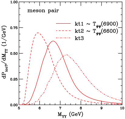
Figure 1: The $T_{\psi\psi}$ probability distribution, calculated using Eq. (2), as a function of mass of the state. Calculations are shown for kt1 (solid), kt2 (dashed), and kt3 (dot-dashed).

The mass distributions for the $X(3872)$ are shown in Fig. 2. The average mass assuming set kt1 for the $k_{T}$ range is 4.3 GeV, significantly larger than the mass of the $X$. However, when the narrower range of set kt2 is used, the average mass is 4.0 GeV, only approximately 0.1 GeV more than the measured mass. In addition, the width in this case is 0.42 GeV, broader than the measured width but resulting in a rather narrow peak nonetheless. Doubling the $k_{T}$ range, with set kt3, results in a broader distribution with a width of $\sim 0.74$ GeV.

Given the rather good agreement with the measured $X(3872)$ mass, most of the calculations of the kinematic distributions in Sec. V will employ this assumption. Exceptions will be made for the $T_{\psi\psi}$ and the $X_{s}$ states which have reported more than one mass state.

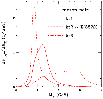
Figure 2: The $X(3872)$ probability distribution, calculated using Eq. (2), as a function of mass of the state. Calculations are shown for kt1 (solid), kt2 (dashed), and kt3 (dot-dashed).

Figure 3 shows the mass distributions of the states labeled $X_{s}$ here, with $c\overline{s}\overline{c}s$ content, effectively a tetraquark state composed of a $D_{s}\overline{D}_{s}$ pair. Based on Table 1, the measured $X_{s}$ states can be approximately grouped into masses of 4.0, 4.55 and 4.7 GeV. To better approximate these masses, set kt4 was introduced with a $k_{T}$ range intermediate between sets kt1 and kt3. Indeed, the calculations shown in Fig. 3 for sets kt2, kt1 and kt4, with average masses of 4.2, 4.5 and 4.9 GeV respectively, are in rather good agreement with these approximate masses. More fine tuning of the $k_{T}$ range could separate individual masses further.

The width increases slowly with the $k_{T}$ range. The widths with sets kt1 and kt2 are similar, 0.43 GeV, while the width with set kt4 is 0.53 GeV. The average mass and corresponding width employing set kt2 is somewhat higher than that for the $X(3872)$ in Fig. 2 because the light $q\overline{q}$ in the 7-particle Fock state for the $X(3872)$ is replaced by the heavier $s\overline{s}$ pair.

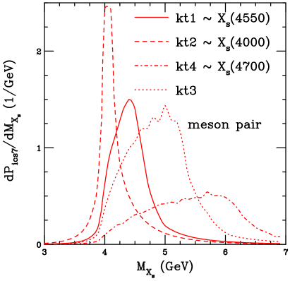
Figure 3: The $X_{s}$ probability distributions, calculated using Eq. (2), as a function of mass of the state. Calculations are shown for kt1 (solid), kt2 (dashed), kt3 (dot-dashed) and kt4 (dotted). The approximately grouped $X_{s}$ masses based on Table 1 are associated with the closest $k_{T}$ range.

Figure 4 compares the mass distributions of the $X(3872)$, $X_{s}$ and $T_{cc}^{-}$ for set kt2. The mass shift between the $X(3872)$ and the $X_{s}$ with $M\approx 4.0$ GeV is apparent, as is the somewhat broader width. The $T_{cc}^{-}$ mass is almost identical to that of the $X(3872)$, as may be expected due to the nearly identical quark content. Its width is also similar, 0.5 MeV compared to 0.4 MeV for the $X(3872)$.

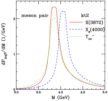
Figure 4: The probability distributions for $X(3872)$ (red solid), $X_{s}$ (blue dashed) and $T_{cc}^{-}$ (dot-dashed green), calculated using Eq. (2), as a function of mass of the state for scenario kt2.

IV.3.2 Mass Distributions Assuming a Four-Quark State

Here the mass distributions of tetraquark states assumed to be composed of loosely bound 4-quark states are shown. These states have either one charm quark or, in the case of $T_{\psi s}$, the $c$ and $\overline{c}$ quarks are assumed to form a “$\psi$” instead of connecting to the light quarks in the state. If they, instead, each connected with a light or strange quark or antiquark, one could consider it to be similar to e.g. the $X(3872)$. Indeed, the reported $T_{\psi s}$ masses in Table 1 are similar to those of the $X_{s}(3960)$ and $X_{s}(4274)$ configured as $c\overline{s}\overline{c}s\equiv D_{s}\overline{D}_{s}$. On the other hand, the $T_{cs}$ states, with one charm quark, are about 1 GeV lighter. The mass distributions are shown for all three nominal $k_{T}$ ranges, sets kt1, kt2 and kt3, in this section.

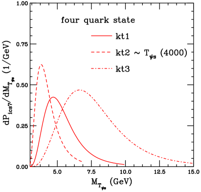
Figure 5: The $T_{\psi s}$ probability distribution, calculated using Eq. (IV.2), as a function of mass of the state. Calculations are shown for kt1 (solid), kt2 (dashed), and kt3 (dot-dashed).

The $T_{\psi s}$ mass distributions are shown in Fig. 5. As in the previous section, the distributions with larger $k_{T}$ ranges have larger average masses. However, now since the quarks are not assumed to pair into mesons but exist in a more loosely bound configuration, the widths are considerably larger, even for the narrowest distribution calculated with set kt2. The average mass with this set, 4.3 GeV, is very similar to that of the $X_{s}$ calculated with set kt2 but the width is now $\sim 0.8$ GeV instead of the value of 0.4 GeV obtained for the $X_{s}$ calculated with the same $k_{T}$ set.

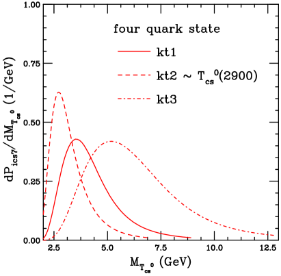
Figure 6: The $T^{0}_{cs}$ probability distribution, calculated using Eq. (IV.2), as a function of mass of the state. Calculations are shown for kt1 (solid), kt2 (dashed), and kt3 (dot-dashed).

Figures 6 and 7 compare the mass distributions calculated from a 7-particle state for $T_{cs0}(2900)^{0}$ and $T_{cs1}(2900)^{0}$ (both labeled $T_{cs}^{0}$ in the figure) and from a 9-particle state for $T^{a}_{c\overline{s}0}(2900)^{0}$ and $T^{a}_{c\overline{s}0}(2900)^{++}$ (both labeled $T_{cs0}^{a}$ in the figure). Recall that in the former case, the antiparticle partner, $\overline{c}d\overline{s}u$, is calculated since producing a $c\overline{d}s\overline{u}$ state in the intrinsic charm model requires a sub-leading 11-particle state.

Despite the additional light $q\overline{q}$ pair required to produce the $T_{cs0}^{a}$, the mass distributions in Fig. 7 are remarkably similar to those of the $T_{cs}^{0}$ in Fig. 6, giving nearly equal masses and very similar widths. In fact, this should not be particularly surprising because employing the same quark flavors in the tetraquark state should yield a similar mass distribution, regardless of how many quarks are in the initial proton wavefunction.

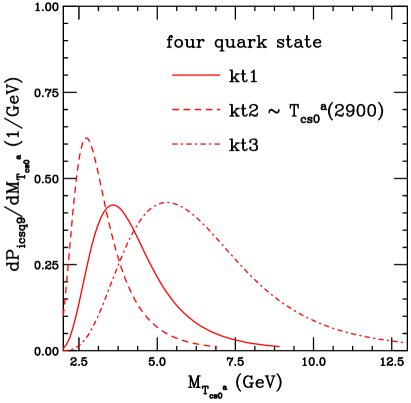
Figure 7: The $T_{cs0}^{a}$ probability distribution, calculated using Eq. (IV.2), as a function of mass of the state. Calculations are shown for kt1 (solid), kt2 (dashed), and kt3 (dot-dashed).

In both cases, the average mass with set kt2 is $\approx 3.3$ GeV, comparable to but slightly larger than the measured mass of the state. The widths, with set kt2, are $\approx 0.9$ GeV, slightly larger than the width calculated for the $T_{\psi s}$.

State	Mass (GeV)
	kt1	kt2	kt3	kt4
Meson pair configuration
$T_{\psi\psi}$	6.933	6.358	7.637	-
$X(3872)$	4.303	4.021	5.236	-
$X_{s}$	4.475	4.215	5.404	4.892
$T_{cc}^{-}$	4.349	4.054	5.394	-
4-quark configuration
$T_{\psi s}$	5.404	4.301	7.716	-
$T_{cs}^{0}$	4.218	3.263	6.261	-
$T_{cs0}^{a}$	4.272	3.288	6.394	-

Table 4: The average tetraquark mass from intrinsic charm states for the $k_{T}$ integration range given. Note that only the $X_{s}$ calculation uses set kt4. Note also that $T_{cs}^{0}$ refers to both $T_{cs1}^{0}$ and $T_{cs0}^{0}$ while $T_{cs0}^{a}$ refers to both $T_{c\overline{s}0}^{a\,0}$ and $T_{c\overline{s}0}^{a\,++}$.

State	Width (GeV)
	kt1	kt2	kt3	kt4
Meson pair configuration
$T_{\psi\psi}$	0.797	0.748	0.905	-
$X(3872)$	0.456	0.422	0.739	-
$X_{s}$	0.431	0.432	0.702	0.534
$T_{cc}^{-}$	0.515	0.510	0.732	-
4-quark configuration
$T_{\psi s}$	1.264	0.783	2.212	-
$T_{cs}^{0}$	1.251	0.883	2.057	-
$T_{cs0}^{a}$	1.270	0.895	2.087	-

Table 5: The width (standard deviation) of the tetraquark mass distribution from intrinsic charm states for the $k_{T}$ integration range given. Note that only the $X_{s}$ calculation uses set kt4. Note also that $T_{cs}^{0}$ refers to both $T_{cs1}^{0}$ and $T_{cs0}^{0}$ while $T_{cs0}^{a}$ refers to both $T_{c\overline{s}0}^{a\,0}$ and $T_{c\overline{s}0}^{a\,++}$.

Overall, the agreement between the calculations and the measured tetraquark candidate masses is quite good. The calculations can also distinguish between assumptions about the nature of the tetraquarks, as either a pair of $D$ or $D_{s}$ mesons or as a more loosely bound 4-quark state. For example, a tetraquark with the composition $c\overline{c}d\overline{s}$ could be arranged either as $(c\overline{s})+(\overline{c}d)\equiv D_{s}^{+}+D^{-}$ or $(c\overline{c})+(d\overline{s})\equiv J/\psi+K^{0}$ In the former case, where the lighter $d$ or $\overline{s}$ quark is associated with a heavy charm quark, the meson pair assumption can be used. In the latter, case, as discussed earlier in this section, one can obtain a defined mass peak only if the state is assumed to be composed of four uncorrelated quarks.

V Tetraquark Kinematic Distributions

The rapidity and $p_{T}$ distributions of the states discussed in the previous section are now calculated. In this section, for ease of calculation, instead of integrating over the tetraquark mass, the average masses are used instead. As in the previous section, all distributions are shown normalized to unity.

The denominator of Eq. (1) ensures that the heaviest quarks in the state carry the largest fraction of the momentum. This can be manifested by the charm quarks either carrying a larger fraction of the longitudinal momentum, represented by Feynman $x$, or $x_{F}$, or larger transverse momentum. The number of quark in the state also plays a role in their kinematic distributions: when the available momentum is distributed among more partons, the average phase space available to each one is reduced.

To demonstrate how the number of quarks in the state might affect the kinematic distributions, in Figs. 8 and 9, the charm quark Feynman $x$ and $p_{T}$ distributions are shown for 5-, 7- and 9-particle states of the proton. To standardize the result, only light $q\overline{q}$ pairs are added to the $|uudc\overline{c}\rangle$ state, i.e. $|uudc\overline{c}q\overline{q}\rangle$ and $|uudc\overline{c}q\overline{q}q\overline{q}\rangle$. Note that $q$ can represent $u$ or $d$ quarks interchangeably because they are assumed to have the same current quark mass in the model.

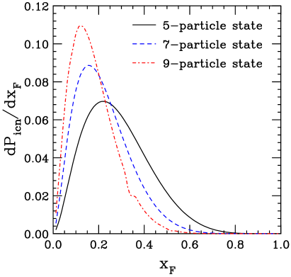
Figure 8: The probability distribution as a function of $x_{F}$ for charm quark production from 5- (solid black), 7- (dashed blue), and 9-particle states (dot-dashed red). All calculations use set kt2.

The $x_{F}$ distribution is shown in Fig. 8 because it is independent of energy and $k_{T}$ range while the rapidity distribution is not. The rapidity distributions, shown later, can also depend on the $k_{T}$ range of the integration since $x_{F}=(2m_{T}/\sqrt{s})\sinh y$. The average $x_{F}$ of the charm quark decreases as the number of quarks in the state. If one adds only light $q\overline{q}$ pairs, the average $x_{F}$ of a charm quark in a 5-quark state ls 0.285, decreasing to 0.220 for a 7-quark state and 0.178 for a 9-particle state. Note that, as a function of rapidity, the boosted distributions would retain the same hierarchy, with charm quarks from a 5-particle state at higher average rapidity than those from a 7- or 9-particle state.

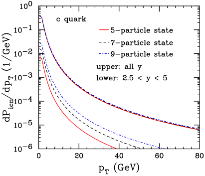
Figure 9: The probability distribution as a function of $p_{T}$ for charm quark production from 5- (solid black), 7- (dashed blue), and 9-particle states (dot-dashed red). All calculations use set kt2. The upper set of curves are integrated over all rapidity while the lower curves correspond to $2.5<y<5$ for $\sqrt{s}=7$ TeV.

The average transverse momentum of a charm quark, integrated over all $x_{F}$ and rapidity, slightly increases with the number of quarks in the state, The increase is likely because the high $p_{T}$ tail of the charm distribution is slightly harder for states with more particles: $\langle p_{T}\rangle=2.32$ GeV for a 5-quark state; 2.37 GeV for a 7-quark state; and 2.40 GeV for a 9-quark state. The charm distribution becomes harder because the additional light quarks in the more populated states have a lower maximum $k_{T}$ range.

As shown in Ref. RV_IC_EN , the $J/\psi$ and $\overline{D}$ meson $p_{T}$ distributions from intrinsic charm depend on the calculated rapidity range. This is demonstrated in Fig. 9 where the charm quark $p_{T}$ distribution integrated over all $x_{F}$ ($0<x_{F}<1$) is compared to that for an $x_{F}$ range appropriate for $2.5<y<5$ at $\sqrt{s}=7$ TeV, corresponding to $0.00454<x_{F}<0.0557$. As can be seen in Fig. 8, because the average $x_{F}$ is reduced for states with more quarks, the $p_{T}$ distribution from a 9-particle state encompasses more of the $p_{T}$ distribution at this low $x_{F}$ than the 5- or 7-particle states.

The assumption of a fixed tetraquark mass in the calculation of the $y$ and $p_{T}$ distributions, in contrast to the mass distributions, means that the calculations are independent of whether the tetraquark is composed of a meson pair or four uncorrelated quarks. Thus the momentum-conserving delta functions and the additional delta functions needed to connect the four constituents of the tetraquark are all that are required in addition to Eq. (1). Thus the kinematic distributions are independent of any correlations between the partons in the state as long as the same number and type of partons are included. This observation was also made in Ref. ANDY .

With this starting point, the rapidity and $p_{T}$ distributions are shown in Secs. V.1 and V.2 respectively.

V.1 Rapidity Distributions

State	$\sqrt{s}$
	5 TeV	7 TeV	13 TeV
$T_{\psi\psi}(6600)$	5.96	6.30	6.91
$T_{\psi\psi}(6900)$	5.40	6.24	6.85
$X(3872)$	6.46	6.80	7.42
$X_{s}$(kt1)	6.32	6.66	7.27
$X_{s}$(kt2)	6.42	6.76	7.39
$X_{s}$(kt3)	6.06	6.39	7.02
$X_{s}$(kt4)	6.21	6.54	7.15
$T_{cc}^{-}$	6.27	6.61	7.23
$T_{\psi s}$	6.42	6.77	7.38
$T_{cs}^{0}$	6.56	6.40	7.51
$T_{cs0}^{a}$	6.34	6.68	7.30

Table 6: The average tetraquark rapidity from intrinsic charm states for different LHC energies. Note that $T_{cs}^{0}$ refers to both $T_{cs1}^{0}$ and $T_{cs0}^{0}$ while $T_{cs0}^{a}$ refers to both $T_{c\overline{s}0}^{a\,0}$ and $T_{c\overline{s}0}^{a\,++}$.

The rapidity distributions are calculated for $\sqrt{s}=5$, 7 and 13 TeV, all center of mass energies for $p+p$ collisions at the LHC. To facilitate comparison between tetraquark states, typically only results are shown for $\sqrt{s}=7$ TeV. The average value of the rapidity is given for all energies in Table 6.

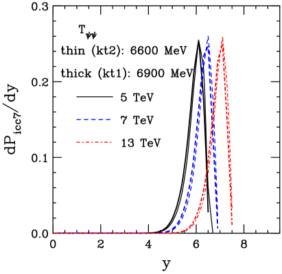
Figure 10: The probability distribution as a function of rapidity for $T_{\psi\psi}$ production at $\sqrt{s}=5$ (solid black), 7 (dashed blue), and 13 TeV (dot-dashed red). The thin lines, for $T_{\psi\psi}(6600)$, use set kt2 while the thick lines, for $T_{\psi\psi}(6900)$, use set kt1.

Figure 10 shows the rapidity distributions for the $T_{\psi\psi}(6600)$ and $T_{\psi\psi}(6900)$, obtained with the $k_{T}$ ranges with sets kt2 and kt1 respectively. As expected, the distributions peak at rapidities greater than 5 with the furthest forward distributions being those at $\sqrt{s}=13$ TeV. Because the $T_{\psi\psi}$ has the largest mass of all the tetraquark candidate states considered, it is boosted least.

The differences between the distributions based on mass ($k_{T}$ range) are negligible on the scale of the plots. They are generally less than 0.1 unit of rapidity given the 300 MeV difference in mass.

All the distributions in this figure and, indeed, all the rapidity distributions shown in this section, have a characteristic shape due to the transformation from $x_{F}$ to rapidity. There is a long tail from zero rapidity until just below the peak where the distribution abruptly climbs. The descent to the edge of phase space above the peak is very abrupt, nearly vertical. This seems almost counterintuitive compared to the charm quark $x_{F}$ distribution where the rise from $x_{F}=0$ to the peak is faster than that descent above it as $x_{F}\rightarrow 1$. However, as noted in the discussion of Fig. 8, at $\sqrt{s}=7$ TeV, while the boost affects all energies similarly, it is less pronounced at lower rapidity.

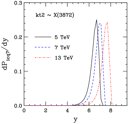
Figure 11: The probability distribution as a function of rapidity for $X(3872)$ production at $\sqrt{s}=5$ (solid black), 7 (dashed blue), and 13 TeV (dot-dashed red), all calculated using parameter set kt2.

The $X(3872)$ rapidity distributions are shown for all three LHC energies in Fig. 11. They are calculated with set kt2, the set of $k_{T}$ integration ranges that agree best with the measured $X(3872)$ mass. While the distributions are similar to those shown in Fig. 10, the lighter mass of the $X(3872)$ results in a more forward-peaked rapidity distribution.

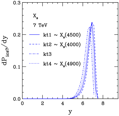
Figure 12: The probability distribution as a function of rapidity for $X_{s}$ production at $\sqrt{s}=7$ TeV for parameter sets kt1 (solid), kt2 (dashed), kt3 (dot dashed) and kt4 (dotted). The approximately grouped $X_{s}$ masses based on Table 1 are associated with the closest $k_{T}$ range.

Figure 12 shows the rapidity distributions for all four sets of $k_{T}$ ranges for the $X_{s}$. Sets kt2, kt1 and kt4 correspond to the states measured at approximately 4.0, 4.5 and 4.9 GeV. The different masses and the associated different $k_{T}$ ranges affect the rapidity distributions. The most forward distribution is found for the narrowest $k_{T}$ range, set kt2, with increasing $k_{T}$ range moving the distribution backward in rapidity so that set kt2 is forward of set kt1, with sets kt4 and kt3 peaking at lower rapidities. The difference in the averages due to the $k_{T}$ range is on the order of 0.1 units of rapidity, similar to the difference noted for the $T_{\psi\psi}$.

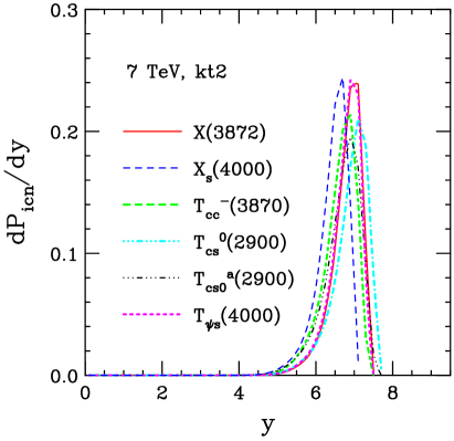
Figure 13: The probability distribution as a function of rapidity at $\sqrt{s}=7$ TeV using parameter set kt2 for $X(3872)$ (solid red), $X_{s}$ (dashed blue), $T_{cc}^{-}$ (dot-dashed green); $T_{cs0}^{a}$ (dot-dot-dot-dashed black), $T_{cs}^{0}$ (dash-dash-dash-dotted cyan) and $T_{\psi s}$ (dotted magenta).

Figure 13 compares all the rapidity distributions for tetraquark candidates with one or two charm quarks at $\sqrt{s}=7$ TeV. All distributions are calculated for set kt2 so that the $X_{s}$ distribution shown corresponds to the lowest mass state. The $X(3872)$, $T_{cc}^{-}$, and $T_{\psi s}$ all have similar quark content (at least two charm quarks) and masses, thus their rapidity distributions are also similar. Note that the exchange of a light quark for a strange quark in the $T_{\psi s}$ does not significantly affect the mass. The $X_{s}$, with two strange quarks, has the lowest average rapidity.

The $T_{cs}^{0}$, with a single charm quark, arising from a 7-particle state, is the most forward. It is worth noting that while the quark content is very similar to that of the $T_{cs0}^{a}$ – one charm quark, one strange quark and two light quarks – the peak of the $T_{cs0}^{a}$ is shifted backward by about 0.2 units of rapidity relative to the $T_{cs}^{0}$. That is because the $T_{cs0}^{a}$ must be produced from a 9-particle state. If a‘non-leading’ 11-particle states had been considered, e.g. to produce the $T_{cc}^{+}$ instead of the $T_{cc}^{-}$, one could expect a similar small backward shift for rapidity distributions from such states even though the quark content and mass are similar. This is clear from Fig. 8.

V.2 Transverse Momentum Distributions

The $p_{T}$ distributions are now shown for the tetraquark candidates, under the same conditions as in Sec. V.1.

		$\sqrt{s}=5$ TeV		$\sqrt{s}=7$ TeV		$\sqrt{s}=13$ TeV
	all $y$	$2.5<y<5$
State	$\langle p_{T}\rangle$	%$P_{{\rm ic},n}$	$\langle p_{T}\rangle$	%$P_{{\rm ic},n}$	$\langle p_{T}\rangle$	%$P_{{\rm ic},n}$	$\langle p_{T}\rangle$
$T_{\psi\psi}(6600)$	4.05	3.40	21.74	1.52	30.32	0.33	47.50
$T_{\psi\psi}(6900)$	4.56	4.52	21.92	2.04	30.45	0.45	47.61
$X(3872)$	2.82	1.36	23.94	0.65	31.82	0.15	48.20
$X_{s}$(kt1)	3.49	2.18	24.19	1.03	32.02	0.24	48.24
$X_{s}$(kt2)	2.97	1.53	24.01	0.73	31.86	0.17	48.13
$X_{s}$(kt3)	4.75	4.36	24.18	2.07	32.12	0.48	48.42
$X_{s}$(kt4)	4.09	3.10	24.33	1.50	32.16	0.35	48.37
$T_{cc}^{-}$	3.93	2.76	24.18	1.34	31.96	0.31	48.15
$T_{\psi s}$	2.98	1.92	24.81	0.93	32.11	0.21	48.29
$T_{cs}^{0}$	3.22	1.83	24.91	0.90	32.46	0.21	48.39
$T_{cs0}^{a}$	3.19	2.94	19.92	1.47	26.48	0.38	41.22

Table 7: The average tetraquark $p_{T}$ (in GeV) from intrinsic charm states for $p+p$ collisions at $\sqrt{s}=5$, 7 and 13 TeV. At each energy, the percentage of the total $p_{T}$ distribution captured in the rapidity range $2.5<y<5$ is given along with the average $p_{T}$ at that energy. The average $p_{T}$ integrated over all rapidity, independent of energy, is also shown. Note also that $T_{cs}^{0}$ refers to both $T_{cs1}^{0}$ and $T_{cs0}^{0}$ while $T_{cs0}^{a}$ refers to both $T_{c\overline{s}0}^{a\,0}$ and $T_{c\overline{s}0}^{a\,++}$.

The $p_{T}$ distributions are again calculated for $\sqrt{s}=5$, 7 and 13 TeV, all center of mass energies for $p+p$ collisions at the LHC. To facilitate comparison between tetraquark states, typically only results are shown for $\sqrt{s}=7$ TeV. The average $p_{T}$ value is given for all energies in Table 7. The averages are first given for the entire forward rapidity range and then assuming that the rapidity range covered is $2.5<y<5$. Because the amount of the total $p_{T}$ distribution captured depends on the rapidity range, the percentage of the total probability for that energy and rapidity range is given as %$P_{{\rm ic},n}$.

While the average $p_{T}$ calculated over all rapidities is rather moderate and similar to the average $p_{T}$ of the charmonium states, albeit somewhat higher, when a finite rapidity region is considered, the average $p_{T}$ increases by an order of magnitude and grows with center of mass energy while the percentage of the $p_{T}$ distribution captured by the rapidity range decreases as the tetraquark candidate is boosted further forward in rapidity as $\sqrt{s}$ increases.

The reason for this is illustrated in Figs. 14 and 15. As shown in Ref. RV_IC_EN , the relation between the Feynman $x$ of the hadron created by coalescence of the constituent quarks in the $J/\psi$, $\overline{D}$ meson, or charm tetraquark candidate, and rapidity means that, for a fixed value of $x_{F}$, the maximum $p_{T}$ can be quite large according to the definition $x_{F}=(2m_{T}/\sqrt{s})\sinh y$.

Because the tetraquark candidate in the intrinsic charm picture is comoving with the parent proton, it can manifest itself at rather high $p_{T}$, even at relatively high rapidity. For example, if $x_{F}=1$ and $m_{T}=1$ GeV, the maximum rapidity is $\sinh^{-1}(\sqrt{s}/2)=8.85$ with $\sqrt{s}=7$ TeV. If $m_{T}=\sqrt{s}/2$, then the maximum rapidity is $y=\sinh^{-1}(1)=0.881$, near midrapidity, for the same energy. At $x_{F}\sim 0$, on the other hand, then $m_{T}\sim 0$ for any rapidity. Thus in Figs. 14 and 15, the $p_{T}$ distribution, integrated over all rapidity, peaks at $p_{T}\sim 0$ and then decreases slowly with $p_{T}$ until near the edge of phase space.

If, on the other hand, one considers a finite rapidity range, the distributions can behave quite differently, as shown in these figures at forward rapidity for $\sqrt{s}=5$, 7 and 13 TeV. The maximum $m_{T}$ in the forward rapidity range covered by LHCb, $2.5<y<5$, is 578.5 GeV for $y=2.5$ and 47.2 GeV for $y=5$, assuming $x_{F}\equiv 1$. Thus the low $p_{T}$ part of the $p_{T}$ spectrum is suppressed at forward rapidity. Increasing the center of mass energy from $\sqrt{s}$ from 5 to 13 TeV consequently increases the suppression of the low $p_{T}$ spectral contribution. However, as the $p_{T}$ increases, the suppression is reduced until, at sufficiently high $p_{T}$ (higher for larger $\sqrt{s}$), the spectrum is no longer suppressed and the distributions merge with that of the rapidity-integrated spectrum. This low $p_{T}$ spectral suppression in a finite rapidity range leads to the large increase in the average $p_{T}$ seen in Table 7. Assuming a lower rapidity range at the same center of mass energies would lead to greater suppression at low $p_{T}$ and increase the average $p_{T}$ still further. The maximum $m_{T}$ is reduced for lower values of $x_{F}$.

Because $m_{T}=\sqrt{p_{T}^{2}+m^{2}}$, for fixed $m_{T}$, a larger mass particle reduces the $p_{T}$ range. The difference in the maximum $p_{T}$ between the $T_{\psi\psi}$ mass of 6.6 or 6.9 GeV and that of the $X(3872)$ is small. However,one can observe a change in the spectral shapes for the $T_{\psi\psi}$ and the $X(3872)$ and, indeed, greater low $p_{T}$ suppression for the more massive state.

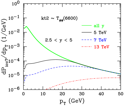
Figure 14: The probability distribution as a function of $p_{T}$ for $T_{\psi\psi}(6600)$ production at $\sqrt{s}=5$ (solid black), 7 (dashed blue), and 13 TeV (dot-dashed red), all calculated using parameter set kt2, corresponding to the mass of $\sim 6600$ MeV.

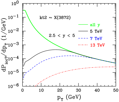
Figure 15: The probability distribution as a function of $p_{T}$ for $X(3872)$ production at $\sqrt{s}=5$ (solid black), 7 (dashed blue), and 13 TeV (dot-dashed red), all calculated using parameter set kt2.

In the remainder of this section, only distributions at $\sqrt{s}=7$ TeV and in the rapidity range $2.5<y<5$ are shown to illustrate differences in the chosen $k_{T}$ ranges and the general makeup of the states themselves.

Figure 16 shows the $p_{T}$ distributions at 7 TeV for the $X_{s}$ states, including all four sets of $k_{T}$ ranges, each calculated with the average mass given in Table 4. It is clear that the larger $k_{T}$ range results in a somewhat harder $p_{T}$ distribution with a slightly higher peak. In the case of the lowest mass and narrowest $k_{T}$ distribution, the percentage of the $p_{T}$ distribution captured in the rapidity range $2.5<y<5$, given as %$P_{{\rm ic},n}$, is the smallest with increasing fractions for sets kt1, kt4 and kt3 respectively, corresponding to broader $k_{T}$ integration ranges. The average $p_{T}$ integrated over all rapidity also increases with increasing $k_{T}$ range, as observed in Table 7. The change in the average $p_{T}$ is much smaller when the rapidity range is fixed to $2.5<y<5$.

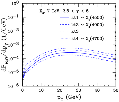
Figure 16: The probability distribution as a function of rapidity for $X_{s}$ production at $\sqrt{s}=7$ TeV for parameter sets kt1 (solid), kt2 (dashed), kt3 (dot dashed) and kt4 (dotted). The approximately grouped $X_{s}$ masses based on Table 1 are associated with the closest $k_{T}$ range.

Finally, the $p_{T}$ distributions for tetraquark candidates with one and two charm quarks are compared in Fig. 17, also at $\sqrt{s}=7$ TeV. Here all the distributions are calculated with set kt2 for more direct comparison. Integrated over rapidity, the average $p_{T}$ values for states with two charm quarks are all around 3 GeV. The average $p_{T}$ of the $T_{cs}^{0}$ and $T_{cs0}^{a}$, with a single charm quark, are somewhat larger but the difference is small. When the rapidity cut is applied, the percentage of the distributions captured are all similar for the $X(3872)$, $X_{s}$, $T_{cc}^{-}$, $T_{\psi s}$ and $T_{cs}^{0}$. However, the values of %$P_{{\rm ic},n}$ are larger overall for the $T_{cs0}^{a}$ because it is produced from a 9-particle state while the others are all produced from 7-particle states. The average $p_{T}$ of the distribution within the rapidity range is also higher, see Table 7. The backward shift to lower $p_{T}$ of the $T_{cs0}^{a}$ distribution is also clear in Fig. 17.

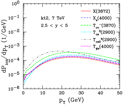
Figure 17: The probability distribution as a function of $p_{T}$ in the rapidity interval $2.5<y<5$ at $\sqrt{s}=7$ TeV using parameter set kt2 for $X(3872)$ (solid red), $X_{s}$ (dashed blue), $T_{cc}^{-}$ (dot-dashed green); $T_{cs1}$ (dot-dot-dot-dashed black), $T_{cs0}$ (dash-dash-dash-dotted cyan) and $T_{\psi s}$ (dotted magenta).

VI Estimated Cross Sections

In this section, the estimated cross sections are briefly discussed. The production cross section for a single intrinsic $c\overline{c}$ pair from a 5-particle $|uudc\overline{c}\rangle$ configuration of the proton can be written as

$$\sigma_{{\rm ic}\,5}(pp)=P_{{\rm ic}\,5}^{0}\sigma_{pN}^{\rm in}\frac{\mu^{2}}{4\widehat{m}_{c}^{2}}\,\,.$$ (4)

The factor of $\mu^{2}/4\widehat{m}_{c}^{2}$ arises from a soft interaction, breaking the coherence of the Fock state, where $\mu^{2}=0.1$ GeV² is assumed, see Ref. VBH1 . The inelastic cross section $\sigma_{pN}^{\rm in}=30$ mb is appropriate for fixed-target interactions and can be used as a conservative value here. Thus, for $P_{{\rm ic},5}^{0}$ between 0.1% and 1%, $3.3\leq\sigma_{{\rm ic}\,5}(pp)\leq 33$ nb.

The cross section for double $J/\psi$ production was estimated in Ref. dblic based on the NA3 double $J/\psi$ production measurements in $\pi^{-}+N$ interactions at pion beam energies of 150 and 280 GeV Badpi and $p+N$ interactions with a proton beam of 400 GeV Badp . Based on the cross sections obtained from these data, for the lowest double intrinsic $c\overline{c}$ state, a 6-particle $|\overline{u}dc\overline{c}c\overline{c}\rangle$ for a $\pi^{-}$ beam and a 7-particle $|uudc\overline{c}c\overline{c}\rangle$ for a $p$ beam, $P_{{\rm icc},7}^{0}$ is between 4.4% and 20% of $P_{{\rm ic},5}^{0}$. Then, for $T_{\psi\psi}$, $X(3872)$, and $T_{cc}^{-}$, all based on a 7-particle state with two intrinsic $c\overline{c}$ pairs, the production cross section is

$$\sigma_{{\rm icc}\,7}(pp)=P_{{\rm icc}\,7}^{0}\sigma_{pN}^{\rm in}\frac{\mu^{2}}{4\widehat{m}_{c}^{2}}\,\,.$$ (5)

Note that the same soft interaction factor is assumed for the 7-particle state and the 5-particle state. Then, given the same range of $P_{{\rm ic},5}^{0}$ as above, $0.14\leq\sigma_{{\rm icc}\,7}(pp)\leq 6.6$ nb.

On the other hand, for $X_{s}$, $T_{\psi s}$, and $T_{cs}^{0}$, the second intrinsic $c\overline{c}$ pair is replaced by an $s\overline{s}$ pair. One could conservatively assume that the probability $P_{{\rm ics},7}$ is larger than $P_{{\rm icc},7}$ by the ratio $(\hat{m}_{c}^{2}/\hat{m}_{s}^{2})\sim 10$, giving $1.4\leq\sigma_{{\rm ics}\,7}(pp)\leq 66$ nb.

Finally, the $T_{cs0}^{a}$ ($T_{c\overline{s}0}^{0}$ and $T_{c\overline{s}0}^{++}$) is based on 9-particle Fock states with intrinsic $c\overline{c}$, $s\overline{s}$ and $q\overline{q}$ pairs where $q$ represents a light quark. Given that the additional $q\overline{q}$ pair is light, there could be no additional penalty so that $P_{{\rm icsq},9}^{0}\approx P_{{\rm ics},7}^{0}$ is a not unreasonable first approximation, leading to $\sigma_{{\rm icsq}\,9}(pp)\approx\sigma_{{\rm ics}\,7}(pp)$.

These cross sections should be taken as estimates of upper limits and not as exact predictions. First, these cross sections encompass all possible charm hadron combinations that could be derived from these 5-, 7- and 9-particle configurations of the proton. These combinatorics have not been worked out here but would reduce the cross sections of individual tetraquarks. Next, if one or more of the components of the tetraquark emerges as a $J/\psi$, the cross section has to be reduced by a factor of $F_{C}\sim 2$% for each emergent $J/\psi$. Thus the $T_{\psi\psi}$ cross section could be reduced by $F_{C}^{2}\sim 4\times 10^{-4}$ to between 0.056 and 2.6 pb while a state like the $T_{\psi s}$ would have the cross section reduced by a single factor of $F_{C}$. These total cross sections do not include any reduction due to phase space acceptance, which can be significant, see Table 7. Finally, it is unclear how much, if at all, the configuration or size of the tetraquark state might affect its cross section, in addition to its width.

VII Summary

The tetraquark mass and kinematic distributions have been studied in terms of the intrinsic charm model. The results suggest that a narrow $k_{T}$ range is compatible with most of the measured tetraquark candidate masses. The mass distributions also suggest that, for tetraquark candidates with one or two charm quark constituents, the $X(3872)$, the $X_{s}$, and the $T_{cc}^{-}$ are compatible with a meson pair structure for the tetraquark while, on the other hand, the $T_{\psi s}$, the $T_{cs}^{0}$ and the $T_{cs0}^{a}$ are more compatible with a loosely bound four-quark configuration.

On the other hand, the kinematic distributions calculated here, are assumed to be independent of the structure. At LHC energies, as studied here, the rapidity distributions are boosted to high rapidity while the $p_{T}$ distributions are very hard, with a high $p_{T}$ tail. These kinematics are considerably different than those obtained in perturbative QCD, as already noted for the $J/\psi$ and $\overline{D}$ mesons RV_IC_EN .

The potential cross sections in this approach are all small but could dominate production in regions of kinematic phase where production by perturbative QCD mechanisms is small, namely at higher rapidity and transverse momentum, as shown in Ref. RV_SMOG for fixed-target $J/\psi$ and $\overline{D}$ production. However, the cross sections given in Sec. VI are total cross sections and do not include any reduction due to finite detector acceptance which could reduce them still further.

Finally, the same basic calculational structure can be applied to bottom tetraquarks, as was already done for a potential $X_{b}(b\overline{b}b\overline{b})$ state in Ref. ANDY . This will be considered in future work.

Acknowledgments A. Angerami and V. Cheung are thanked for discussions. This work was supported by the Office of Nuclear Physics in the U.S. Department of Energy under Contract DE-AC52-07NA27344 and the LLNL-LDRD Program under Project No. 23-LW-036, and the HEFTY Collaboration.

References

- (1) S. K. Choi et al. [Belle Collaboration], Observation of a narrow charmonium-like state in exclusive decays, Phys. Rev. Lett. 91, 262001 (2003).
- (2) M. Ablikim et al. [BESIII Collaboration], Observation of a Charged Charmonium-like Structure in at GeV, Phys. Rev. Lett. 110, 252001 (2013).
- (3) Z. Q. Liu et al. [Belle Collaboration], Study of and Observation of a Charged Charmonium-like State at Belle, Phys. Rev. Lett. 110, 252002 (2013).
- (4) A. V. Evdokimov et al. [SELEX Collaboration], First observation of a narrow charm-strange meson and , Phys. Rev. Lett. 93, 242001 (2004).
- (5) T. Aaltonen et al. [CDF Collaboration], Evidence for a Narrow Near-Threshold Structure in the Mass Spectrum in Decays, Phys. Rev. Lett 102, 242002 (2009).
- (6) V. M. Abazov et al. [D0 Collaboration], Evidence for a state, Phys. Rev. Lett. 117, 022003 (2016).
- (7) V. M. Abazov et al. [D0], Study of the state with semileptonic decays of the meson, Phys. Rev. D 97, 092004 (2018).
- (8) G. Aad et al. [ATLAS Collaboration], Observation of an Excess of Dicharmonium Events in the Four-Muon Final State with the ATLAS Detector, Phys. Rev. Lett. 131, 151902 (2023).
- (9) A. Hayrapetyan et al. [CMS Collaboration], Observation of new structure in the J/J/ mass spectrum in proton-proton collisions at = 13 TeV, [arXiv:2306.07164 [hep-ex]].
- (10) R. Aaij et al. [LHCb Collaboration], Observation of structure in the -pair mass spectrum, Sci. Bull. 65, 1983-1993 (2020).
- (11) R. Aaij et al. [LHCb], Observation of a Resonant Structure near the Threshold in the Decay, Phys. Rev. Lett. 131, 071901 (2023).
- (12) R. Aaij et al. [LHCb], Observation of structures consistent with exotic states from amplitude analysis of decays, Phys. Rev. Lett. 118, 022003 (2017).
- (13) R. Aaij et al. [LHCb], Observation of New Resonances Decaying to + and , Phys. Rev. Lett. 127, 082001 (2021).
- (14) R. Aaij et al. [LHCb], Observation of an exotic narrow doubly charmed tetraquark, Nature Phys. 18, 751-754 (2022).
- (15) R. Aaij et al. [LHCb], Evidence of a Structure in Decays, Phys. Rev. Lett. 131, 131901 (2023).
- (16) R. Aaij et al. [LHCb], First Observation of a Doubly Charged Tetraquark and Its Neutral Partner, Phys. Rev. Lett. 131, 041902 (2023).
- (17) R. Aaij et al. [LHCb], Amplitude analysis of the decay, Phys. Rev. D 102, 112003 (2020).
- (18) https://www.nikhef.nl/ pkoppenb/particles.html
- (19) S. J. Brodsky, P. Hoyer, C. Peterson, and N. Sakai, The Intrinsic Charm of the Proton, Phys. Lett. B 93, 451 (1980).
- (20) S. J. Brodsky, C. Peterson, and N. Sakai, Intrinsic Heavy Quark States, Phys. Rev. D 23, 2745 (1981).
- (21) J. Badier et al. [NA3 Collaboration], Evidence for Production in Interactions at 150 GeV/ and 280 GeV/, Phys. Lett. B 114, 457 (1982).
- (22) J. Badier et al. [NA3 Collaboration], Production and Limits on Beauty Meson Production From 400 GeV/ Protons, Phys. Lett. B 158, 85 (1985).
- (23) R. Vogt and S. J. Brodsky, Intrinsic charm contribution to double quarkonium hadroproduction, Phys. Lett. B 349, 569 (1995).
- (24) L. C. Bland et al. [ANDY Collaboration], Observation of Feynman scaling violations and evidence for a new resonance at RHIC, [arXiv:1909.03124 [nucl-ex]].
- (25) R. Vogt and A. Angerami, Bottom tetraquark production at RHIC?, Phys. Rev. D 104, 094025 (2021).
- (26) M. Karliner, J. L. Rosner and S. Nussinov, states: masses, production and decays, Phys. Rev. D 95, 034011 (2017).
- (27) Z.-G. Wang, Analysis of the tetraquark states with QCD sum rules, Eur. Phys. J. C 77, 432 (2017).
- (28) Y. Bai, S. Lu and J. Osborne, Beauty-full Tetraquarks, Phys. Lett. B 798, 134930 (2019).
- (29) J. Wu, Y.-R. Liu, K. Chen, X. Liu and S.-L. Zhu, Heavy-flavored tetraquark states with the configuration, Phys. Rev. D 97, 094015 (2018).
- (30) G. Yang, J. Ping, L. He and Q. Wang, Potential model prediction of fully-heavy tetraquarks (), [arXiv:2006.13756 [hep-ph]].
- (31) X. Z. Weng, X. L. Chen, W. Z. Deng and S. L. Zhu, Systematics of fully heavy tetraquarks, Phys. Rev. D 103, 034001 (2021).
- (32) S. J. Brodsky, P. Hoyer, A. H. Mueller, and W.-K. Tang, New QCD production mechanisms for hard processes at large , Nucl. Phys. B 369, 519 (1992).
- (33) S. Paiva, M. Nielsen, F. S. Navarra, F. O. Duraes and L. L. Barz, Virtual meson cloud of the nucleon and intrinsic strangeness and charm, Mod. Phys. Lett. A 13, 2715 91998).
- (34) M. Neubert, Heavy quark symmetry, Phys. Rept. 245, 259 (1994).
- (35) F. M. Steffens, W. Melnitchouk, and A. W. Thomas, Charm in the nucleon, Eur. Phys. J. C 11, 673 (1999).
- (36) T. J. Hobbs, J. T. Londergan and W. Melnitchouk, Phenomenology of nonperturbative charm in the nucleon, Phys. Rev. D 89, 074008 (2014).
- (37) J. Pumplin, H. L. Lai, and W. K. Tung, The Charm Parton Content of the Nucleon, Phys. Rev. D 75, 054029 (2007).
- (38) P. M. Nadolsky et al., Implications of CTEQ global analysis for collider observables, Phys. Rev. D 78, 013004 (2008).
- (39) S. Dulat et al., Intrinsic Charm Parton Distribution Functions from CTEQ-TEA Global Analysis, Phys. Rev. D 89, 073004 (2014).
- (40) P. Jimenez-Delgado, T. J. Hobbs, J. T. Londergan and W. Melnitchouk, New limits on intrinsic charm in the nucleon from global analysis of parton distributions, Phys. Rev. Lett. 114, 082002 (2015).
- (41) R. D. Ball et al. [NNPDF Collaboration], A Determination of the Charm Content of the Proton, Eur. Phys. J. C 76, 647 (2016).
- (42) J. Blum̈lein, A kinematic condition on intrinsic charm, Phys. Lett. B 753, 619 (2016).
- (43) S. J. Brodsky, A. Kusina, F. Lyonnet, I. Schienbein, H. Spiesberger, and R. Vogt, A review of the intrinsic heavy quark content of the nucleon, Adv. High Energy Phys. 2015, 341547 (2015).
- (44) S. J. Brodsky, G. I. Lykasov, A. V. Lipatov and J. Smiesko, Novel Heavy-Quark Physics Phenomena, Prog. Part. Nucl. Phys. 114, 103802 (2020).
- (45) R. S. Sufian, T. Liu, A. Alexandru, S. J. Brodsky, G. F. de Téramond, H. G. Dosch, T. Draper, K. F. Liu and Y. B. Yang, Constraints on charm-anticharm asymmetry in the nucleon from lattice QCD, Phys. Lett. B 808, 135633 (2020).
- (46) G. A. Alves et al. [E769 Collaboration], Enhanced leading production of and in 250 GeV -nucleon interactions, Phys. Rev. Lett. 72, 812 (1994).
- (47) E. M. Aitala et al. [E791 Collaboration], symmetries between the production of and mesons from 500 GeV/ -nucleon interactions as a function of and , Phys. Lett. B 371, 157 (1996).
- (48) M. Adamovich et al. [WA82 Collaboration], Study of and Feynman’s distributions in -nucleus interactions at the SPS, Phys. Lett. B 305, 402 (1993).
- (49) LHCb Collaboration, Open charm production and asymmetry in Ne collisions at GeV, arxiv:2211.11633.
- (50) R. Vogt and S. J. Brodsky, Charmed hadron asymmetries in the intrinsic charm coalescence model, Nucl. Phys. B 478, 311 (1996).
- (51) R. Vogt, Contribution from intrinsic charm production to fixed-target interactions with the SMOG Device at LHCb, Phys. Rev. C 108, 015201 (2023).
- (52) T. Gutierrez and R. Vogt, Leading charm in hadron nucleus interactions in the intrinsic charm model, Nucl. Phys. B 539, 189 (1999).
- (53) R. Vogt, Energy dependence of intrinsic charm production: Determining the best energy for observation, Phys. Rev. C 106, 025201 (2022).
- (54) R. Vogt, Limits on Intrinsic Charm Production from the SeaQuest Experiment, Phys. Rev. C 103, 035204 (2021).
- (55) R. Vogt, S.J. Brodsky, and P. Hoyer, Systematics of Production, Nucl. Phys. B 360, 67 (1991).